Hybrid Metaheuristics Applied to Image Reconstruction for an Electrical Impedance Tomography Prototype

Abstract

Evolutionary computation has much scope for solving several important practical applications. However, sometimes they return only marginal performance, related to inappropriate selection of various parameters (tuning), inadequate representation, the number of iterations and stop criteria, and so on. For these cases, hybridization could be a reasonable way to improve the performance of algorithms. Electrical impedance tomography (EIT) is a non-invasive imaging technique free of ionizing radiation. EIT image reconstruction is considered an ill-posed problem and, therefore, its results are dependent on dynamics and constraints of reconstruction algorithms. The use of evolutionary and bioinspired techniques to reconstruct EIT images has been taking place in the reconstruction algorithm area with promising qualitative results. In this chapter, we discuss the implementation of evolutionary and bioinspired algorithms and its hybridizations to EIT image reconstruction. Quantitative and qualitative analyses of the results demonstrate that hybrid algorithms, here considered, in general, obtain more coherent anatomical images than canonical and non-hybrid algorithms.

1 Introduction

From the several areas of computational intelligence, evolutionary computation has been emerging as one of the most important sets of problems for solving methodologies and tools in many fields of engineering and computing [1,2,3,4,5]. When compared to other optimization techniques, learning processes based on population, self-adaptation, and robustness appear as fundamental aspects of evolutionary algorithms in comparison to other optimization techniques [1,2,3].

Despite the large acceptance of evolutionary computation to solve several important applications in several fields such as engineering, e-commerce, business, economy, and health, they tend to return marginal performance [1,2,3]. Such limitation is related to the large numbers of parameters being selected (the tuning problem), inadequate data representation, the number of iterations, and stop criteria. Nevertheless, according to the No Free Lunch theorem, it is not possible to find the best optimization algorithm for solving all problems with uniform performance (i.e. for all algorithms); high performance over a determined set of problems is compensated by medium and low performance in all other problems [1, 2]. Therefore, taking into account all possible problems, the overall performance for all possible optimization algorithms tends to be the same [1, 6,7,8].

Evolutionary algorithm behavior is governed by interrelated aspects of exploitation [1, 2]. Such aspects point to limitations that could be overcome by the use of hybrid evolutionary methods dedicated to optimizing the performance of direct and classical evolutionary approaches [1,2,3,4,5]. The hybridization of evolutionary algorithms has become relatively widespread due to their ability to deal with a considerable amount of real world complex issues usually constrained by some degrees of uncertainty, imprecision, interference, and noise [4, 5, 9, 10].

Academia and industry have been paying increasing interest to non-invasive imaging techniques and health applications [11, 12], since imaging diagnosis techniques and devices based on ionizing radiation methods could be related to the occurrence of several health problems due to long exposure, like benign and malignant tissues and, consequently, cancer, one of the most important public health problems, both for developed and under-developed countries [11, 12].

Electrical impedance tomography (EIT) is a low-cost, portable, and safely handled non-invasive imaging technique free of ionizing radiation, offering a considerably wide field of possibilities [13]. Its fundamentals are based on the application of electrical currents to a pair of electrodes on the surface of the volume of interest [13,14,15,16], returning electrical potentials used in tomographic image reconstruction, that is finding the distribution of electrical conductivities, by solving the boundary value problem [15, 16]. Since this is an ill-posed problem, there is no unique solution, that is there is no warranty to obtain the same conductivity distribution for a given distribution of electrical potentials on surface electrodes [13, 16].

Boundary value problems can be solved using optimization problems by considering one or more target metrics to optimize. Taking into account this principle, the EIT reconstruction problem can be solved by the effort to minimize the relative reconstruction error using evolutionary computation, where individuals (solution candidates) are probable conductivity distributions. The reconstruction error is defined as the error between the experimental and calculated distributions of surface voltages.

In this chapter we propose a methodology to solve the problem of reconstruction of EIT images based on hybrid evolutionary optimization methods in which tuning limitations are compensated by the use of adequate heuristics. We perform simulations and compare experimental results with ground-truth images considering the relative squared error. The evaluation of quantitative and qualitative results indicate that the use of hybrid evolutionary and bioinspired algorithms aid the avoidance of local minima and obtain anatomically consistent results, side-stepping the use of empirical constraints as in common and non-hybrid EIT reconstruction methods [17], in a direct and relatively simple way, despite their inherent complexity.

This chapter is organized as follows. In Sect. 2 we present a review on evolutionary computation and bioinspired algorithms, with special focus on swarm intelligence; in Sect. 3 we present a review on density-based fish school search, a bioinspired swarm algorithm based on fish school behavior; in Sect. 4 we briefly present a Gauss–Newton electrical impedance tomography reconstruction method; some comments on hybridization are presented in Sect. 6; in Sect. 5 we present a bibliographical revision of EIT, image reconstruction problems, and software tools for image reconstruction based on finite elements; in Sect. 7 we present our proposed EIT image reconstruction methodology based on hybrid heuristic optimization algorithms, as well as the experimental approach and infrastructure; in Sect. 8 we present the experimental results and some discussion; since EIT is a relatively new imaging technique, we also present a hardware proposal in Sect. 9; finally, in Sect. 10 we make more general comments on methodology and results.

2 Heuristic Search, Evolutionary Computation, and Bioinspired Algorithms

Evolutionary computation is one of the main methodologies that compose computational intelligence. The algorithms of evolutionary computation (called evolutionary algorithms) were inspired by the evolution principles from genetics and elements of Darwin’s Theory of Evolution, such as natural selection, reproduction, and mutation [18].

The main goal of evolutionary computing is to provide tools for building intelligent systems to model intelligent behavior [18]. Since evolutionary algorithms are non-expert iterative tools, that is they are not dedicated to a specific problem, having a general nature that makes possible their application to a relatively wide range of problems, they can be used in optimization, modeling, and simulation problems [19].

An evolutionary algorithm is a population-based stochastic algorithm. According to [19], the idea behind evolutionary algorithms is the same: given a population of individuals embedded in some resource-constrained environment, competition for such resources causes natural selection, where better adapted individuals succeed in surviving, reproducing and perpetuating its characteristics (survival of the fittest). As the generations go by, the fitness of the population increases toward the environment. The environment represents the problem itself, an individual a possible solution (also called a solution candidate), the fitness of an individual represents the quality of the solution to the problem in question, and generations represent the iterations of the algorithm [19, 20]. The way in which these algorithms solve problems is called trial-and-error (also known as generate-and-test) [19]. Following evolutionary concepts, possible solutions to the problem are generated and evaluated for the problem in question. In order to get even better solutions, some of them are chosen to be combined by generating new candidates for the solution.

Besides evolutionary algorithms, computational intelligence also uses bioinspired algorithms. These two types of algorithms differ from each other by the inspiration or metaphor taken into account for its development. While evolutionary algorithms take into account the theories of genetics and evolution, the other one takes into account the behavior of living things in nature, such as the collective behavior of birds in searching for food. The brute-force proposal generate-and-test is the same for both algorithms; however, bioinspired algorithms do not have recombination, mutation, and selection operators. In spite of that, they have operators which simulate intelligent behavior.

Some examples of bioinspired algorithms are: Particle Swarm Optimization (PSO), based on the behavior of birds in searching for food [21]; the Bacterial Foraging Algorithm, inspired by the social foraging behavior of the bacterium Escherichia coli present in the human intestine [22]; the Search for Fish School (FSS) [23]; and Density based on Fish School Search (dFSS) [24], based on the collective behavior of fish in searching for food. Some of these types of algorithm are also based on insect behavior: Ant Colony Optimization (ACO) [25] and Artificial Bee Colony [26, 27]. In the following subsections some of these algorithms that were applied in the reconstruction of EIT images are presented.

2.1 Particle Swarm Optimization

PSO is a bioinspired method for search and optimization inspired by a flock’s flight in search of food sources and the shared knowledge among the flock’s members. The method was created by mathematically modeling the birds as particles, their flight as direction vectors, and their velocity as continuous values [21].

As in the bird’s flock flight, the particles move toward the food source influenced by two main forces: its own knowledge and memory of where to go, and the leader’s experience. The leader is commonly the bird which is most experienced, and in the mathematical model it is the solution candidate that best fits the approached function [21]. The velocity and weight distribution updating is done according to the following expressions (1) and (2).

$$\displaystyle \begin{aligned} v_{i}(t+1)= \omega(t) v_{i}(t) + c_1(t) r_1(t) (p_i-x_i(t))+ c_2(t) r_2(t) (p_g-x_i(t)) {} \end{aligned} $$

(1)

$$\displaystyle \begin{aligned} x_i(t+1) = x_i + v_i(t+1) {} \end{aligned} $$

(2)

where v _i(t + 1) is the velocity vector of the i-th particle; ω(t) is the inertia factor; c ₁ and c ₂ are the individual influence and the social factor, modeling the strength of the particle’s own experience and that of the leader, respectively; and r ₁(t), r ₂(t) ∼ U[0, 1].

Along the iterative process, the particles have their configuration updated by receiving the mathematical influence of the best configuration found so far (modeling the leader influence), and the best configuration ever found by the particle itself (modeling its own experience). There is also an inertia factor, which is a number, generally less than 1, that decreases the velocity of the particle at each iteration, modeling the reduction of the velocity when the particle gets close to the optimal configuration. In Table 1 we show the general PSO algorithm.

Table 1 Particle swarm optimization

In the first step, the particles are initialized as vectors containing ‘Dim’ positions each. Each position is normally initialized with a random number, in the range of domain of the approached problem.

The second phase is to initialize the velocities. They are vectors with the same dimension of the particles and in the same quantity of the particles. Each velocity vector corresponds to a particle and each position of this vector corresponds to one position (weight) of this particle.

The third and 5.III phases calculate the objective function for each particle and create a rank with the evaluation of each particle. Those evaluations will be used in the following step.

In steps 4 and 5.II, GBest is identified, which is the best particle found so far (by evaluation through the objective function), and Pbest is identified, which for each particle is the best configuration found so far.

Finally in the 5.II phase, the particle weights are updated by their respective velocity vector and are calculated as in the expression (1).

The PSO algorithm, as approached in this work, is used to reconstruct EIT images by modeling solution candidates as particles, as described in Sect. 7.

The hybrid technique will evolve the insertion of one of the particles that will be generated by the Gauss–Newton algorithm.

2.2 Simulated Annealing

Simulated annealing (SA) is a stochastic approach for the global optimization of a given function based on local search and hill climbing. It is a metaheuristic optimization algorithm to deal with large discrete search spaces [28]. SA could be preferable to gradient-descent methods when reaching an approximate global optimum is more important than finding a precise local optimum, given a determined time interval [28].

Its metaheuristic is inspired by annealing in metallurgy, in which heating and controlled cooling of a material is employed to increase the size of its crystals and reduce their defects, affecting both the temperature and the thermodynamic free energy. The process of slow cooling is interpreted as a slow decrease in the probability of accepting the worse solutions, thus improving exploration capabilities [28]. In each iteration, a solution close to the current one is selected and evaluated. Afterwards, the algorithm decides to accept or reject the current solution, taking into account the probabilities of the newly calculated solution being better or worse than the present solution. The temperature is progressively decreased, converging from an initial positive value to zero, which affects the probabilities. Probabilities are calculated as described in Eq. (3). The general behavior of SA algorithms is given by the pseudocode of Table 2, adapted to solve the EIT image reconstruction problem [29]. The symbolic function GenerateRandomNeighbor(S) is responsible for obtaining a neighbor solution in the search space of the current solution (S) and depends on the problem to be solved.

$$\displaystyle \begin{aligned} P(\varDelta E) = e^{-\frac{\varDelta E}{kT}} \end{aligned} $$

(3)

Table 2 The pseudocode of a Simulated Annealing algorithm

Table 3 The pseudocode of a Differential Evolution algorithm

where P(ΔE) is the probability of keeping a state that produces a thermal energy increase of ΔE (as in statistical mechanics) in the objective function; k is a parameter analogous to Stefan–Boltzman’s Constant, usually assumed to be 1; and T is the temperature defined by a cooling scheme, the main parameter of the process control. The probability of a particular state decreases with its energy as temperature increases. This fact can be observed in the reduction of the slope of P(ΔE) [29]. Additionally, it is possible to demonstrate that, as SA converges to the global minimum, a very slow temperature reduction is observed, requiring a considerably large amount of iterations [28].

2.3 Differential Evolution

After presenting the Chebychev Polynomial Problem by Rainer Storn, Kenneth Price (1995) in attempting to solve this problem created Differential Evolution (DE) when he had the idea of using different vectors to recreate the population vector. Since then, a number of tests and substantial improvements have been made which has resulted in DE becoming a versatile and robust Evolutionary Computation algorithm [30, 31].

2.3.1 Stages of Differential Evolution

According to [30], DE is characterized by its simplicity and efficiency at solving global optimization problems in continuous spaces. Similar to Genetic algorithms, DE benefits from diversity combined operators of mutation and crossover, in order to generate individuals modeled as vectors, which are candidates for the next generation. The new population is defined by the selection mechanism, selecting the individuals to survive for the next population according to simple criteria. In this process, the population size remains constant. Therefore, the individuals of generation G are modeled as real vectors, x _i,G, i = 1, 2, …, N _P, where N _P is the population size [32].

The optimization process is governed by the following:

• The algorithm is initiated by creating a randomly chosen initial population with uniform distribution, corresponding to the vectors of unknown parameters (potential solutions), taking into account the search space limit [30]. Typically, the unknown parameters are conditioned by lower and upper boundary constraints, $x_{j}^{(L)}$ e $x_{j}^{(U)}$, respectively, as in the following:

  $$\displaystyle \begin{aligned} x_{j}^{(L)} \leq x_j \leq x_{j}^{(U)}, j = 1, 2, \dots, D. {} \end{aligned} $$

  (4)

  Therefore, the initial population is defined as:

  $$\displaystyle \begin{aligned} x_{j,i}^{(0)} = x_{j}^{(L)} + r_j[0,1]\cdot (x_{j}^{(U)} - x_{j}^{(L)}) {} \end{aligned} $$

  (5)

  where, i = 1, 2, …, N _P, j = 1, 2, …, D, and r _j ∼ U[0, 1].

• In DE, new individuals are generated by three individuals, related as following. For each individual x _i,G, i = 1, 2, …, N _P, a basic DE mutant vector (classical) is generated according to:

  $$\displaystyle \begin{aligned} v_{i,G+1} = x_{a,G} + F(x_{b,G} - x_{c,G}), {} \end{aligned} $$

  (6)

  where the random indexes a, b, c ∈{1, 2, …, N _P} and a ≠ b ≠ c. The amplification parameter F ∼ U(0, 2] controls the amplification of the differential variation (x _b,G − xc, G). However, there are some other variant mutation operations, as shown in Table 4.

  Table 4 Main strategies of the Differential Evolution technique

  A potential reason for DE to acquire reasonable results is that the mutation operator is governed by the difference between the coordinates of the individuals of the current population [30]. Consequently, each parameter is automatically exchanged and appropriately reduced, aiding convergence to the desired approximate solution.

• The mutated vector is mixed with the target vector to produce the trial vector, formed as in the following:

  $$\displaystyle \begin{aligned} w_{i,G+1} = \left\{ \begin{array}{ll} v_{i,G+1}, & r_j\leq CR~~~\vee~~~j = k(i)\\ x_{i,G}, & r_j > CR~~~\vee~~~j \neq k(i) \end{array} \right., {} \end{aligned} $$

  (7)

  where j = 1, 2, …, D, i = 1, 2, …, N _P, r _j ∼ U[0, 1], and k(i) ∈ 1, 2, …, D is a randomly chosen index, which ensures that w _i,G+1 receives at least one coordinate of v _i,G+1. The parameter CR ∈ [0, 1] is the crossing constant, set by the user [30].

• The individual of the new generation is selected as the better evaluated vector from the trial vector w _i,G+1 and the target vector x _i,G, according to the objective function [30].

• The iterative process finishes when a determined number of iterations is reached or a predetermined value of the objective function is obtained with a considerably small error [30].

• The population size N _P is chosen from 5D to 10D and is kept constant during the search process. Parameters F and CR are set during the search process and affect the speed of convergence and robustness. Appropriate values for NP, F, and CR are usually empirically determined [30].

The optimization process is detailed in the pseudocode of DE algorithms, designed to minimize an objective function $f_0: \mathbb {R}^n \rightarrow \mathbb {R}$, where P _CR is the probability of crossing [33,34,35,36], shown in Table 3.

2.3.2 Differential Evolution Strategies

The strategies of DE consist of different variation operators, and can be nominated according to the following acronym: DE/a/b/c, where [32]:

a::

Specifies the vector to be disturbed, which can be “rand” (a vector of the randomly selected population) or “best” (the least cost vector of the population);

b::

Determines the number of weighted differences used for the perturbation of a;

c::

Denotes the type of crossings (exp: exponential; bin: binomial).

Price [37] suggested 10 different strategies and some work guidelines for using them. These strategies were derived from the five different DE mutation regimes. Each mutation strategy was combined with the “Exponential” or “Binomial” crossover, providing 5 × 2 = 10 DE strategies. Nevertheless, other combinations of linear vectors can be used for the mutation. In Table 4 we have Prive’s 10 DE strategies [37].

The α, β, γ, ρ, and δ indexes are mutually exclusive integers chosen randomly in the range [1, n], where n is the number of agents of the initial population, and all are different from the old base index. These indexes are randomly generated once for each donor vector. The scale factor F _p is a positive control parameter for the expansion of the difference vectors. $X_{best}^{(q)}$ is the agent vector with the best aptitude (i.e. the lowest objective function value for a minimization problem) in the generation population q.

2.4 Fish School Search

The FSS was developed by Bastos Filho and Lima Neto in 2008. Such a method takes into account the protection and realization of the mutual achievements of oceanic fish [23], where the real characteristics of the fish that served as inspiration for the method can be classified as feeding and swimming. In the first characteristic, it is considered that fish possess the natural instinct to seek food; such a characteristic is incorporated into the algorithm to indicate the success of fish (those who find more feed are more successful). In the second characteristic, the capacity of the fish to move individually and in a flock (shoal) is taken into account, where the search for feed is one of the reasons why fish move.

Therefore, the process of FSS is performed by a population of individuals with limited memory—the fish [23]. Each fish in the shoal represents a possible solution to the optimization problem [23]. This method is recommended for high-dimension search and optimization problems [23, 24]. Considering the characteristics of feeding and swimming, the algorithm is formed by four operators, being one of feeding (the weight) and three of swimming (the operators of movement), which are described in the following sections.

2.4.1 Individual Movement Operator

Considering fish’s individual capacity for searching for food, the individual movement operator is responsible for moving the fish to a random region of its neighborhood; this movement does not consider the influence of the other fish of the school for its realization. An important feature of such a movement is that the fish moves only in the positive direction of the fitness function, that is it travels only if the random position is better than the current position.

The individual displacement of each fish i, $\varDelta x_{ind_{i}}$ is given in Eq. (8), where rand(−1, 1) is a vector of random values uniformly distributed in the range [−1, 1], and step _ind is the individual movement step, a parameter that represents the ability of the fish to move in the individual movement. After calculating the individual displacement the position of fish $x_{ind_{i}}$ is updated through Eq. (9).

$$\displaystyle \begin{aligned} \varDelta x_{ind_{i}}(t+1) = step_{ind}\cdot rand(-1,1) {} \end{aligned} $$

(8)

$$\displaystyle \begin{aligned} x_{ind_{i}}(t+1) = x_{ind_{i}}(t) + \varDelta x_{ind_{i}}(t+1) {} \end{aligned} $$

(9)

In order to guarantee the convergence of the algorithm during the search process, the value of the parameter step _ind decreases linearly as shown in Eq. (10), where $step_{ind_i}$ and $step_{ind_f}$ are the initial and final values of step _ind, and iterations is the maximum possible value of iterations of the algorithm.

$$\displaystyle \begin{aligned} step_{ind}(t+1) = step_{ind}(t) - \frac{step_{ind_i} - step_{ind_f}}{\textit{iterations}} {} \end{aligned} $$

(10)

2.4.2 Feeding Operator

The weight of the fish is the indicator of its success, that is the more food the fish finds, the more successful the fish is, which represents a better solution in the optimization problem [24, 38]. In this way, weight is the function to be maximized by the search process. The fish’s weight is given as a function of the variation of the fitness function generated by the individual movement (Δf _i), as shown in the equation below:

$$\displaystyle \begin{aligned} W_{i}(t+1) = W_{i}(t) + \frac{\varDelta f_i}{\max(\varDelta f)} {} \end{aligned} $$

(11)

where W _i(t) and W _i(t + 1) represent the weight of the i fish before and after the update.

2.4.3 Collective Instinctive Movement Operator

The first collective movement to be considered in FSS is the collective-instinctive movement, where the most successful fish in the individual movement guides the other fish to the points of greatest food encountered by it. Such motion is carried out through the resulting direction vector I(t), that is the weighted average of the individual displacements ξ. Having as weight the individual fitness variance Δx _i, the expression for that mean is given in Eq. (12), where N represents the number of fish in the shoal. Then, the new position of all fish is obtained following Eq. (13).

$$\displaystyle \begin{aligned} I(t) = \frac{\sum_{i=1}^{N} \varDelta x_{ind_i}\varDelta f_i}{\sum_{i=1}^{N} \varDelta f_i} {} \end{aligned} $$

(12)

$$\displaystyle \begin{aligned} x_{i}(t+1) = x_{i}(t) + I(t) {} \end{aligned} $$

(13)

2.4.4 Collective Volitive Movement Operator

The following and last collective movement, the collective-volitional movement, is based on the performance of all fish in the school [39]. In this movement, the fish may move towards the center of mass of the shoal or move away from it. The calculation of the center of mass of the school, Bary(t), is done according to Eq. (14).

The choice whether the fish will approach or move away from the center of mass is made by analyzing whether the fish are gaining weight during the search process. If the fish, in general, are increasing in weight, it means that the search is being successful and the fish approach each other, decreasing the radius of the search; in this case, the movement is carried out following Eq. (15). Otherwise, if the fish are losing weight, the search is unsuccessful and the fish move away from each other, increasing the search radius, executing the movement through Eq. (16). In Eqs. (15) and (16), the parameters rand(0, 1) represent a vector of random values evenly distributed in the range [0, 1], and step _vol is the step of the collective-volitional movement.

$$\displaystyle \begin{aligned} Bary(t) = \frac{\sum_{i=1}^{N} x_{i}W_{i}(t)}{\sum_{i=1}^{N} W_{i}(t)} {} \end{aligned} $$

(14)

$$\displaystyle \begin{aligned} x(t+1) = x(t) - step_{vol} \cdot rand(0,1) (x(t) - Bary(t)) {} \end{aligned} $$

(15)

$$\displaystyle \begin{aligned} x(t+1) = x(t) + step_{vol} \cdot rand(0,1) (x(t) - Bary(t)) {} \end{aligned} $$

(16)

3 Density Based on Fish School Search

Based on the FSS, the Density based on Fish School Search (dFSS) is an algorithm dedicated to the optimization of multimodal functions proposed by Madeiro, Bastos-Filho, and Lima Neto [24, 38]. In the method, the main Fish School is divided into Sub-Fish Schools of different sizes, so that each sub-group will explore different regions of the aquarium, which have possible solutions to the problem. Unlike the other methods discussed here, which get only one solution at the end of their runs, on dFSS it is possible to obtain a set of global and local optimal solutions. In fact, the function of the relative quadratic error for TIE is multimodal, but since the objective of the reconstruction is to obtain only one image, the application of dFSS to TIE is done by considering as a solution the best image obtained by the method in relation to the objective function.

In addition to the feeding and movement operators of the search for Fish schools adapted to the multimodal approach, dFSS has two more operators, the memory and partitioning operators, which will be dealt with in more detail later in this section.

In dFSS the food purchased by a fish is shared with the other fish of the shoal. The amount of shared food from one fish i to another fish j, C(i, j) is given by Eq. (17), where q _ij is the number of fish k that satisfy the relationship d _ik < d _ij (density of fish around the fish i), including fish i, and $d_{R_{ij}} = {d_{ij}}/{[\forall k \neq i \mathrm{,} \min (d_{ik})]}$ is the normalized distance. Then, the updating of the weight of each fish will take into account the total food that was shared with it, as given by Eq. (18), where Q represents the number of fish that were successful during the individual movement. Different from what happens in nature, in the dFSS proposal it is assumed that the weight of the fish does not decrease over the iterations [24].

$$\displaystyle \begin{aligned} C(i,j) = \frac{\varDelta f_i}{(d_{R_{ij}})^{q_{ij}}\sum_{k=1}^{N}{\frac{1}{(d_{R_{ik}})^{q_{ik}}}}} {} \end{aligned} $$

(17)

$$\displaystyle \begin{aligned} W_{i}(t+1) = W_{i}(t) + \sum_{j=1}^{Q}C(i,j) {} \end{aligned} $$

(18)

Food sharing is responsible for the control and maintenance of different sub-Fish Schools, since each fish cooperates (sharing its success) with the other fish around them, the most significant sharing is with the closest fish and in regions less populous. This is modeled by the index $(d_{R_{ij}})^{-q_{ij}}$ greater is the value of q _ij (i.e. the denser the region around the fish i), smaller will be the quantity shared for the fish j [24]. Further detail on the formation of sub-shoals is given in the explanation of the memory and partitioning operators in the following paragraphs.

Individual movement in the dFSS occurs in the same way as in the FSS, but for segregation of the main fish school the adjustment of the movement parameter has been modified. The new way of updating the step of the individual movement is given by Eqs. (19), (20), (21), and (22), where decay _i is the decay rate, $decay_{\min } \in [0,1]$, $decay_{\max }$ are the minimum and maximum decay rates, respectively, $decay_{\max _{init}}$, $decay_{\max _{end}} \in [0,1]$ are the initial and final maximum decay rates, respectively, and must obey the following condition: $decay_{\max _{end}} < decay_{\max _{init}} < decay_{\min }$, and finally $T_{\max }$ is the maximum number of iterations [24, 38]. The initial value of the individual step is given by the parameter step _init, that is $step_{ind_i}(0) = step_{init}$ [24].

$$\displaystyle \begin{aligned} step_{ind_i}(t+1) = decay_i \cdot step_{ind_i}(t) {} \end{aligned} $$

(19)

$$\displaystyle \begin{aligned} decay_i = decay_{\min} - \left( \frac{R_{i}(t)-\min(R_{j}(t))}{\max(R_{j}(t)) - \min(R_{j}(t))} \right)(decay_{\min} - decay_{\max}(t)) {} \end{aligned} $$

(20)

$$\displaystyle \begin{aligned} decay_{\max}(t) = decay_{\max_{init}} \left(\frac{decay_{\max_{end}}}{decay_{\max_{init}}} \right)^{{t}/{T_{\max}}} {} \end{aligned} $$

(21)

$$\displaystyle \begin{aligned} R_i(t) = \sum_{j=1}^{Q}\frac{\varDelta f_j}{(d_{R_{ij}})^{q_{ij}} \sum_{k = 1}^{N}\frac{1}{\left(d_{R_{jk}}\right)^{q_{jk}}}} {} \end{aligned} $$

(22)

In the dFSS each fish has a memory M _i = {M _i1, M _i2, …, M _iN}, where N is the total number of fish. In a fish’s memory is the information of how much food the other fish have shared with it throughout the search process. The index M _ij indicates the influence of fish j on fish i, that is, the larger the M _ij the greater the influence of fish j on fish i. The memory operator is calculated by Eq. (23), where ρ ∈ [0, 1] is the forgetting rate, a parameter that controls how the influence exerted on past iterations is remembered.

$$\displaystyle \begin{aligned} M_{ij}(t+1) = (1 - \rho)M_{ij}(t) + C(j,i) {} \end{aligned} $$

(23)

The collective-instinctive movement of dFSS is similar to the Fish School search, although each fish has its own resulting direction vector I _i which is given by the weighted average of the displacement performed on the individual movement by a fish j having as weight its influence M _ij as shown in Eq. (24). The fish position update is given by Eq. (25). According to [24], even the fish that did not move during the individual movement will influence the result of I _i, causing fish i to simulate this behavior by remaining stationary according to the value of M _ij.

$$\displaystyle \begin{aligned} I_i(t) = \frac{\sum_{j=1}^{N}{\varDelta x_j M_{ij}}}{\sum_{k=1}^{N}{M_{ik}}} {} \end{aligned} $$

(24)

$$\displaystyle \begin{aligned} x_i(t+1) = x_i(t) + I_i(t) {} \end{aligned} $$

(25)

After the execution of the collective-instinctive movement the partitioning operator responsible for the division of the main school into several sub-schools of different sizes is executed. For the division of the school, the following belonging condition is taken into account: a fish i belongs to the same sub-school of fish j only if i is the fish that exerts the greatest influence on fish j or vice versa [24]. The division process begins when a randomly chosen fish i is removed from the main school to form a new sub-shoal, then another fish j is sought where i is the most influential for j or vice versa; if there is a j that satisfies this condition it will be removed from the main shoal and added to the sub-school in question; then this procedure is repeated for fish j in a cascade process. This process is repeated until no more fish that satisfy the condition of belonging to that particular sub-school are found. When this happens a new fish from the main shoal will be randomly removed to compose a new sub-school and the process resumes. The formation of the sub-shoals is carried out until there are no more fish in the main shoal [24].

Finally, the collective-volitional movement is performed independently for each sub-school as given in Eq. (26). In this movement all the fish move towards the barycenter of the sub-shoal (Bary _k(t)) to which it belongs. The barycenter of each sub-school is calculated in the same way as FSS, given in Eq. (14). To avoid premature convergence, the magnitude of the pitch to be performed by the fish towards the barycenter varies according to the value of $decay_{\max }(t)$ [24]. The pseudocode of the dFSS method [38] is shown in Table 5.

$$\displaystyle \begin{aligned} x(t+1) = x(t) + (1 - decay_{\max}(t))(Bary_k(t) - x(t)) {} \end{aligned} $$

(26)

Table 5 The pseudocode of density based on Fish School Search algorithm

4 The Gauss–Newton Method

Based on Newton’s method (dedicated to estimating roots of a function) the Gauss–Newton method is an algorithm which has been widely used in the reconstruction of EIT images [40, 41]. This method, implemented to eliminate the use of second derivatives, consists of a gradient-descent-based numerical method used to solve non-linear least squares problems minimizing the sum of quadratic functions [41]. The application of the Gauss–Newton method in EIT is done by estimating a conductivity distribution σ _k which minimizes the expression given in (27), where $\phi _{ext,k}(\overrightarrow {u}) = f(I(\overrightarrow {u}), \sigma _k(\overrightarrow {v}))$, for all $\overrightarrow {u} \in \partial \varOmega$ and $\overrightarrow {v} \in \varOmega$ [41].

$$\displaystyle \begin{aligned} s_k = \frac{1}{2} \sum_{u \in \partial \varOmega} (\phi_{ext,k}(\overrightarrow{u}) - \phi_{ext}(\overrightarrow{u}))^2 {} \end{aligned} $$

(27)

The hybridizations done in this work evolve the Gauss–Newton method, working together with the techniques presented before. The nomenclature used to describe a hybrid technique in this works is ‘technique’ with Non Blind Search (NBS) or ‘technique’-NBS. For instance, the hybrid approach with the PSO and the Gauss–Newton algorithm will be called a PSO a with non-blind search, or PSO-NBS.

5 Electrical Impedance Tomography

EIT is a promising imaging technique that is non-invasive and free of ionizing radiations. This technique reconstructs images of the inside of a body (or any object) through electrical quantities measured below its surface. For this, electrodes are placed across a transverse section of a body. These electrodes are connected with a control and data acquisition system that is responsible for the application of a pattern of an alternated and low amplitude electrical current and also for the measurement of the border electrical potentials that are generated by this stimulus. When collected, the electrical current and potential data are conveyed to a computer that makes the image reconstruction [42, 43].

The images obtained by EIT are the computational reproduction of an estimated mapping of electrical properties inside a section of body that are calculated through the relation between the stimulus data and response data. By electrical properties, in this case, is understood electrical conductivity or permissiveness; electrical conductivity is the measurement of how easy a material conducts electricity and electrical permissiveness is the measurement of how easy electrical charges of a material are separated under the application of an electric field. A good conductor allows passage of continuous and alternated current whereas a high permissiveness material allows the passage only of alternated current [44]. The tissues and organs of the human body, due to its constitution, have characteristic values of conductivity and permissiveness. Factors such as concentration of water, ions, and blood irrigation determine whether a tissue or an organ is less or more conductive or permissive. This justifies the use of EIT in the medical field, because the difference of conductivity and permissiveness between organs supplies the necessary contrast in the EIT image for differentiation of these organs.

Nowadays, the medical imaging field has very well consolidated techniques such as X-rays, computed tomography, nuclear magnetic resonance, and positron emission tomography. Despite that, EIT has advantages when compared to these other methods that makes it a promising technique in medical imaging. These advantages are:

• EIT does not use ionizing radiation, hence is harmless to patients [44]. Thus, it is viable for performing this technique several times or even for continuous use in monitoring certain functionalities of a body.

• EIT has small dimensions [45], which allows the device to be moved to the patient and even used in the patient’s bed in intensive care units.

• EIT has low cost when compared to other imaging techniques.

Although these advantages make EIT a promising technique, it is still recent and not strongly established, presenting low-resolution images and slow reconstruction when compared to other tomography techniques [46, 47], which makes it not fully reliable for medical diagnosis.

The process of reconstructing EIT images is divided into two problems: the direct problem and the inverse problem [46, 47]. In the direct problem, the conductivity distribution of the inner domain and the current are known and the objective is to determine an electric potential distribution at the internal and boundary (edge) points of the domain [45]. This process is governed by Poisson’s equation and its boundary conditions for the EIT problem. In the inverse problem, the goal is to estimate the internal conductivity distribution of a domain knowing the pattern of the current excitation and the edge potentials due to this excitation. The inverse problem, mathematically, is a non-linear, poorly placed and poorly conditioned problem [42, 48], because more than one solution is possible for this problem for the same input values, that is small data measurement errors can lead indefinitely to large errors in the solution [42, 48]. This factor makes EIT imaging quite dependent on the reconstruction method used.

From a mathematical point of view, the field of study of EIT, that is the section for which the image is desired, can be considered to be a closed 2D region Ω where its boundary surface is given by ∂Ω as shown in Fig. 1.

Fig. 1

EIT domain

To reduce the complexity of this problem it is considered that the image domain should consist of an isotropic medium.¹ However, the electrical nature of human organs and tissues is anisotropic² [49, 50]. Despite the proposed hypothesis being wrong, it is necessary, due to the limited knowledge about this topic in EIT and related areas [49].

Taking into account a low-frequency excitation current (of the order of 125 kHz) the permissiveness effect can be disregarded [51]. Thus, the electric medium is considered to be conductive σ(x, y) because, when considering low frequencies, the inductive and capacitive effects can be ignored [52]. Therefore, the current density $\overrightarrow {J}$ generated from an injected electric current is given by Eq. (28) [51].

$$\displaystyle \begin{aligned} \overrightarrow{J} = \sigma \overrightarrow{E} {}\end{aligned} $$

(28)

where $\overrightarrow {E}$ represents the medium’s electric field. Considering that the excitation frequency value is lower than 30 MHz, it has the following [53]:

$$\displaystyle \begin{aligned} \overrightarrow{E} = -\nabla \phi {} \end{aligned} $$

(29)

$$\displaystyle \begin{aligned} \nabla \cdot \overrightarrow{J} = 0 {}\end{aligned} $$

(30)

where ∇ is the symbol nabla that denotes the gradient operator,³ ∇⋅ is the divergent operator⁴ and ϕ(x, y) represents the internal electric potential at a point (x, y) of the domain Ω. Thus, replacing Eqs. (29) and (30) in Eq. (28) yields Poisson’s equation, given in (31), which relates the conductivity values and electrical potentials of a domain [51, 53].

$$\displaystyle \begin{aligned} \nabla \cdot(\sigma \nabla \phi) = 0 {} \end{aligned} $$

(31)

Poisson’s equation has unlimited solutions, which means that for a given electrical potential distribution there are several conductivity distributions that satisfy Eq. (31). The number of solutions is limited by boundary conditions inherent to the problem. In EIT, the electrical currents are injected only by electrodes placed around the patient, which means that in specific positions on the domain’s surface the following boundary condition can be taken into account:

$$\displaystyle \begin{aligned} \sigma \frac{\partial \phi(\sigma)}{\partial \hat{n}} = \left\{ \begin{array}{rll} J_i, & i = 1,2,3, \ldots, n_e \\ 0, & \text{in other points of } \partial \varOmega \end{array}\right. {} \end{aligned} $$

(32)

where n _e is the number of electrodes used and $\hat {n}$ is a normal versor⁵ on the domain’s edge and outside oriented. Following the same line, the known electrical potentials are the ones arranged on a domain’s contour, measured by the electrodes. In this way, the second contour condition for this problem is the following:

$$\displaystyle \begin{aligned} \phi_{ext}(x,y) = \phi(x,y), \quad \forall (x,y) \in \partial \varOmega {} \end{aligned} $$

(33)

where ϕ _ext(x, y) is the electrical potential distribution measured by the electrodes.

Determination of the electric potential distribution measured by electrodes ϕ _ext(u, v), knowing the electric current of excitation I(u, v), and distribution of internal conductivity σ(x, y), is called the direct problem of EIT. It is defined by Eq. (31) and the boundary conditions (32) and (33) [51]. The direct problem can be modeled by the relation given in Eq. (34).

$$\displaystyle \begin{aligned} \phi_{ext}(u,v) = f(I(u,v), \sigma(x,y)), \quad \forall (u,v) \in \partial\varOmega \wedge (x,y) \in \varOmega {} \end{aligned} $$

(34)

The inverse problem, however, is the reconstruction of EIT images themselves [42]. The objective is to determine an internal conductivity distribution σ(x, y) in the domain by knowing the excitation current I(u, v) and the edge potentials measured at the electrodes ϕ _ext(u, v). This problem is considered the inverse of the function given in Eq. (34), being modeled conformed in Eq. (35).

$$\displaystyle \begin{aligned} \sigma(x,y) = f^{-1}(I(u,v), \phi_{ext}(u,v)), \quad \forall (u,v) \in \partial\varOmega \wedge (x,y) \in \varOmega {} \end{aligned} $$

(35)

Then, the direct problem is to solve Poisson’s equation (31) knowing the internal conductivity distribution of a domain and the boundary condition given in Eq. (32) for the injected current. The inverse problem consists of the resolution of Eq. (31) knowing the two boundary conditions given by Eqs. (32) and (33), but not knowing the conductivity distribution [54].

The inverse problem of EIT is an intrinsically ill-posed problem because it does not have a unique solution, that is several conductivity distributions would respond to the current excitation at the same distribution of measured electrical potentials. According to [49], if measurements were made with infinite precision and over the entire surface of the domain, the problem would have a unique solution. However, in the imaging process the data are discretely sampled and noisy, causing a loss of information. Besides that a large variation of conductivity can produce only a small variation in discrete measurements. Thus, the ideal would be to use as many electrodes as possible. It was found that by increasing the number of electrodes it is possible to improve the ill-posed condition of this problem and consequently the quality of the reconstructed images [55]. However, it has also been noted that increasing the number of electrodes significantly increases the reconstruction time [55]. In addition to that, the number of electrodes is limited by the measurement area and the size of the electrodes [56]. The inverse problem is also ill-conditioned because small oscillations in the measurements (such as noise) can produce large oscillations in the final non-linear solution, because changes in conductivity values of the domain do not produce a linear change in the values of the surface potentials [49].

5.1 Objective Function

The use of evolutionary and bioinspired algorithms in the reconstruction of EIT images occurs when approaching the reconstruction problem as an optimization problem. For this it is necessary that an objective function be optimized. In this chapter, is used as objective function the relative squared error given in Eq. (36), where n _e is the number of electrodes, V  is the electrical potential distribution measured on the electrodes, and U(x) is the electrical potential distribution of a random image x that is a candidate for the solution considered in the algorithm [57].

$$\displaystyle \begin{aligned} f_{o}(x) = \left[ \frac{\sum_{i = 1}^{n_e}{(U_{i}(x) - V_i)^2}}{\sum_{i = 1}^{n_e}{(V_i)^2}} \right]^{1/2} {} \end{aligned} $$

(36)

$$\displaystyle \begin{aligned} V = (V_1 \mathrm{,} V_2 \mathrm{,} \ldots \mathrm{,} V_{n_e})^T, \end{aligned} $$

(37)

$$\displaystyle \begin{aligned} U(x) = (U_1(x) \mathrm{,} U_2(x) \mathrm{,} \ldots \mathrm{,} U_{n_e}(x))^T \end{aligned} $$

(38)

5.2 Electrical Impedance Tomography and Diffuse Optical Tomography Reconstruction Software

Electrical Impedance Tomography and Diffuse Optical Tomography Reconstruction Software (EIDORS) is an open source software developed at MATLAB and Octave. The experiments presented in this chapter were performed using EIDORS, which has functions capable of solving the direct problem of EIT and the creation of finite element meshes[58].

6 Hybridization

Hybridization consists in using more than one technique in cooperation to solve a determinate problem, although if one technique can solve the approached problem in a satisfactory way, there is no necessity for hybridization. The use of hybridization is justified when the interaction among two or more techniques can improve the performance of the problem resolution.

There are mainly three types of hybrid system. They are:

• Sequential hybrid system: The technique is used in a pipeline way.

• Auxiliary hybrid system: These are techniques co-working to help one technique to solve a determinate problem. The accessory technique is used, normally, to improve the stages of the main technique.

• Embedded hybrid system: The evolved techniques are integrated. They work together as equals to approach the solution of a problem.

The hybridization described in this work are embedded, once the Gauss–Newton method is responsible for including a solution into the pool of solution candidates of each technique, which is intended to guide the search and to avoid falling in local minimals. The results are shown for EIT image reconstruction, by using raw techniques, such as particle swarm algorithms and density based on the Fish School Search; Also shown are the results of the collaborative work of each one with the Gauss–Newton model as new hybrid approaches.

6.1 Differential Evolution Hybridized with Simulated Annealing

According to [59] the DE method which has a stronger global search character, only a few generations are sufficient to find a solution close to the ideal. However, according to its algorithm, each generation requires the selection, crossing, and mutation of the agents of the current population, thus requiring a high computational cost, that is a high number of calculations of the objective function. The SA method is a local search algorithm with a high convergence speed due to the fact that it is able to avoid local minima [60, 61]. In this direction, the proposal of this work is a hybrid version of DE based on simulated annealing (DE-SA), which consists of the implementation of DE and adding SA within the selection operator to improve ED global search capacity.

Pseudocode

• 1. Initialization: Generate the initial population of n random agents D dimensional, each represented by a vector X _j,i,G = rand _j,i[0, 1], where j = 1, 2, …, NP; G is the current generation; and F _i = rand(0, 2] is the mutation scale factor for each individual.

• 2. Set the value of P _CR;

• 3. Population Mutation: The population mutation is based on the strategy of DE/best/1/bin. As shown in Table 4,

  $$\displaystyle \begin{aligned}V_{j,i,G} = X_{j,best,G} + F_i(X_{j,i_1,G} - X_{j,i_2,G})\end{aligned} $$

  where i ₁ ≠ i ₂ ≠ i and X _j,best,G corresponds to the most suitable agent in the current generation.

• 4. Population Crossing: Population crossing is based on the DE binomial crossing operation, as shown by the equation of Table 4.

  $$\displaystyle \begin{aligned}W_{j,i,G} = \begin{cases} V_{j,i,G},\ if\ (rand_{j,i}(0,1)\ \leq\ P_{CR}\ or\ j = j_{rand})\\ X_{ji,G},\ {\mathrm{otherwise}} \end{cases}\end{aligned} $$

• 5. Population selection: This is processed by comparing the target vector X _j,i,G with the vector of judgment W _j,i,G of the population. In addition, SA is added inside the selection operator, and t _G represents the ambient temperature of the current generation.

  $$\displaystyle \begin{aligned} t_{G+1} = \frac{t_G}{1+G \sqrt{t_G}} \end{aligned} $$

  (39)
  $$\displaystyle \begin{aligned} x_{i,j,G+1} = \begin{cases} W_{j,i,G}, & \text{if}\ \ f_0(W_{j,i,G}) \leq f_0(W_{j,i,G})\\ W_{j,i,G}, & \text{if}\ \ f_0(W_{j,i,G}) > f_0(W_{j,i,G}) \\ & \text{and}\ \ rest\left(\frac{G}{4}\right) = 0 \\ & \text{and}\ \ f_0(W_{j,best,G}) = f_0(W_{j,best,G-1}) \\ & \text{and}\ \ f_0(W_{j,best,G}) = f_0(W_{j,best,G-2}) \\ & \text{and}\ \ \exp \left[- \frac{(f_0(W_{j,i,G})- f_0(W_{j,i,G}))}{t_G} \right] > rand(0,1)\\ W_{j,i,G}, & \mathrm{Otherwise} \end{cases} {} \end{aligned} $$

  (40)

  where W _j,best,G is the fittest agent of the current generation, X _j,best,G−1 is the fittest agent of generation (G − 1) and X _j,best,G−2 is the fittest agent of generation (G − 2). Every four generations, these conditions are implemented to assess whether the value of the objective function of the best candidate for the solution has assumed a local minimum in the last three generations. In this case, the judgment vector W _j,i,G can be maintained for the next generation if it satisfies the condition imposed by the exponential expression based on the probability of the SA optimization process.

• 6. Stop if the stop criterion is satisfied. Otherwise, go back to Step 3.

Recall that P _CR is the probability of crossing and f ₀ corresponds to the objective function. Also for the DE-SA method, the initial agents were defined with a normal distribution of random conductivity in the range [0, 1].

6.2 Fish School Search Hybridization

According to the discussion in Sect. 2.4, one can observe that the FSS algorithm is quite dependent on the individual movement operator and therefore the parameter step _ind decreases linearly with the iterative process.

With the proposal to increase the refined search between the intermediary and final iterations, we changed the linear decay for an exponential decay. In this way, the step _ind value decays faster, thus the algorithm will execute a more refined search, that is the algorithm will execute a more exploitative and less exploratory search.

The equation for the exponential decay was made in such a way that the step _ind value continues, beginning with $step_{ind_i}$ and ending with $step_{ind_f}$. This expression is given in Eq. (41).

$$\displaystyle \begin{aligned} step_{ind}(t) = step_{ind_i} \times \exp \left[\frac{t}{N}\ln\left(\frac{step_{ind_f}}{step_{ind_i}} \right) \right] {} \end{aligned} $$

(41)

7 Methodology

In the EIT reconstruction simulations our goal was to identify a conductive object within a circular non-conductive domain. We considered three cases where the object was placed in the center, between the center and the edge, and at the edge of the domain. These images, called ground-truth images, were created by using EIDORS with a mesh of 415 finite elements and 16 electrodes. Figure 2 shows the ground-truth images used in the experiments.

Fig. 2

Ground-truth images for the object placed (a) in the center (b), between the center and the edge, and (c) at the edge of the circular domain

For all methods here discussed we used Eq. (36) as the objective function, where each dimension of the vector (solution candidate) corresponds to a particular finite element on the mesh. The stop criterion utilized was the maximum number of iterations.

The parameter used in the PSO for the experiments were: ‘c1’and ‘c2’ = 2; ω (inertia weight) = 0.8; number of iterations = 500; and number of particles = 100.

For the DE’ implementations, the agent referred to by the DE-SA algorithm is represented by a numerical vector containing the internal conductivity values of a candidate for the solution, that is the agent is a candidate for solving the TIE problem. The parameters used to implement the DE-SA method were initial number of agents: 100, probability of crossover: 90%, initial temperature: 200,000, and number of iterations: 500.

The parameters used for FSS’ methods were 100 fish, W ₀ = 100, $step_{ind_i} = 0.01$, $step_{ind_f} = 0.0001$, step _volt = 2step _ind and iterations= 500. Whereas for dFSS’ methods they were ρ = 0.3, step _init = 0.01, $decay_{\min } = 0.999$, $decay_{\max _{init}} = 0.99$, $decay_{\max _{end}} = 0.95$, and $T_{\max } = 500$.

8 Experimental Results and Discussion

In this section, the results obtained by reconstruction of EIT images through the use of hybrid methods previously described are presented.

8.1 Particle Swarm Optimization

The PSO and Gauss–Newton/PSO reconstructed images are shown in this section. They are presented in two results categories, which are:

• Qualitative: Figures 3 and 4 are the reconstructed images for the three ground-truths (center, between the center and the border, and the border) for the canonical PSO and the same technique with a particle generated by the Gauss–Newton algorithm inserted at the beginning of the iterative process, respectively.

  Fig. 3

  

  Particle swarm optimization reconstructed images. Center ground-truth: ‘a’; between the center and the border ground-truth: ‘b’; and border ground-truth: ‘c’. The numbers at the right side of the chars (1, 2, and 3) stand for 50, 300, and 500 iterations, respectively

  Fig. 4

  

  Particle swarm optimization with non-blind search reconstructed images. Center ground-truth: ‘a’; between the center and the border ground-truth: ‘b’; and border ground-truth: ‘c’. The numbers at the right side of the chars (1, 2, or 3) stand for 50, 300, and 500 iterations, respectively

• Quantitative: The graphs, shown in Figs. 5, 6, and 7 are the evolution of the relative error of the best particle, calculated by the objective function presented in Sect. 5.1, along the 500 iterations of each of the three executions of the algorithms for the center, between the center and the border, and the border ground-truth images, respectively.

  Fig. 5

  

  Relative error for the ground-truth center placed

  Fig. 6

  

  Relative error for the ground-truth placed between the center and the border

  Fig. 7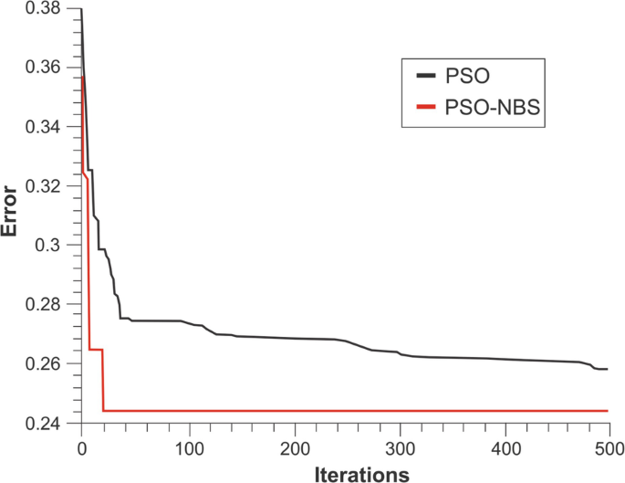

  

  Relative error for the ground-truth border placed

8.1.1 Particle Swarm Optimization and with Non-blind Search Qualitative Discussion

As with the results, their discussion is also qualitatively and quantitatively separated.

The qualitative analysis considers images reconstructed and several aspects of the similarity with their respective ground-truth (Fig. 2) and the noise presence and cleanness of the circular domain.

The images generated by the PSO in Fig. 3 are generally noisier than the ones generated by the hybrid technique (PSO-NBS). It is important to clarify that by noisier we mean a less isolated resistive area (in red) with several artifacts around it. That means that the technique could not generate images with good isolation of the searched object (ground-truth). The same happened for the three ground-truth configurations.

On the other hand, the images generated by the PSO with non-blind search (Fig. 4) are cleaner than the former ones (by isolating the red object, which is the ground-truth). This factor means that the inclusion of a particle with prior knowledge, generated by the Gauss–Newton algorithm, can improve significantly the quality of the generated images.

In these experiments, the only drawback of the hybrid approach was when the image to be reconstructed was placed at the border of the domain (c1, c2, and c3). The reconstructed resistive area (in red) was slightly different from its ground-truth (Fig. 2 circular domain ‘c’). Nevertheless, these images are still in better shape and with a better noise level than the ones generated with only the Particle Swarm Algorithm.

Under this analysis, it is clear that, qualitatively, the PSO-NBS hybrid approach (Fig. 4) overcame the only PSO approach (Fig. 3) in all the aspects.

8.1.2 Particle Swarm Optimization and with Non-blind Search Quantitative Discussion

The quantitative analysis is based on the capacity of finding a low relative error value and the capacity of escaping local minimals along the iterations. Those factors can be observed in the relative error plots.

Under the three configurations (Figs. 5, 6 and 7), the hybrid approach (PSO-NBS, in red) shows a capacity of finding deeper values (i.e. lower relative error values). This probably happens because of the guidance of the search when a Gauss–Newton generated particle is put into the swarm. Besides, it is possible to notice that, unlike the PSO (in black), the PSO-NBS, in most of the cases, is able to escape local minimal regions. This can be seen by the linear trajectory of the back line in Fig. 5 around 150 iterations and in Fig. 6 around 340 iterations, when the error stops falling. The PSO-GN also has this trend of stagnating the error’s fall; however, before that happens, this technique had already found a lower error than the PSO in the three cases.

The reconstruction problem regarding the border reconstruction images by the hybrid approach is also present in the quantitative results. In Fig. 7, the PSO-NBS (in red) stops its evolution (i.e. relative error falling) near the 20th iteration, which characterizes a local minimal stack, and therefore generation of a non-clear isolation of the searched object, as seen in Fig. 7, sub-units c1, c2, and c3. That is also the reason for those three images being equal, as there was no improvement (finding a better image) after the 20th iteration.

8.2 Differential Evolution Hybridized with Simulated Annealing

The results obtained for the hybridized reconstruction method are compared with the classical methods of DE and SA. The pseudocode and the characteristics of these methods were presented in Sect. 6.1.

It is important to remember that the initial agents were defined as having a random internal conductivity distribution in the range [0, 1] in the DE-SA method.

The results in Figs. 8 and 9 show images obtained from the DE and hybrid DE-SA method for an isolated object located in the center, between the center and the edge, and at the edge.

Fig. 8

Reconstructions obtained from the DE method for an isolated object located in the center (a1, a2, a3), between the center and the edge (b1, b2, b3), and near the edge (c1, c2, c3) of the circular domain for 50, 300, and 500 iterations, respectively

Fig. 9

Reconstructions obtained from the hybrid DE-SA method for an isolated object located in the center (a1, a2, a3), between the center and the edge (b1, b2, b3), and near the edge (c1, c2, c3) of the circular domain for 50, 300, and 500 iterations, respectively

Where the situation represented in (a)–(c) is the location of an object in the center, between the center and the edge, and near the edge, respectively. (a1), (a2), and (a3) represent the images of the best candidates for solution of the object in the center in 50, 300, and 500 iterations, respectively. (b1), (b2), and (b3) represent the image of the best candidate for solution of the object between the center and the edge in 50, 300, and 500 iterations. Represents the image of the best candidate for solution to the object in near the edge in 50, 300, and 500 iterations.

Comparing the images given in Figs. 8 and 9, one can say that DE-SA can identify the objects with only 50 iterations; on the other hand, DE is able to identify only the case where the object is placed at the edge. Indeed, DE-SA obtained images are anatomically consistent and conclusive from 300 iterations for the three ground-truth images. Qualitatively, the DE-SA method showed high capacity in generating images with few artifacts from 300 iterations for all configurations, thus is a potential technique for eliminating image artifacts.

Figure 10 shows the graph for the error decrease in the function of the number of iterations for the DE and DESA methods. The curves in blue, red, and green represent the results for the object placed in the center, between the center and the edge, and at the edge, respectively, and the continuous and dotted lines represent the DE and DE-SA results, respectively.

Fig. 10

Graph of the value of the objective function by number of iterations for DE and DE-SA

From the graph in Fig. 10, we can observe that DE-SA always obtained lower results than DE, showing that the hybrid technique succeeds the non-hybrid technique. In this way, the comparison of the DE-SA method with the traditional method of DE shows that the former was more efficient in reconstruction, generating consistent images with a low relative noise level in the first 50 iterations. The reconstructions obtained with the DE-SA technique presented a greater edge definition when compared with the traditional method.

8.3 Exponential Hybridization of the Fish School Search

In this section the results for the hybridization of the FSS algorithm where the parameter step _ind is updated following an exponential function as discussed in Sect. 6.2 will be presented.

In Figs. 11 and 12 reconstructed images are shown for the FSS and for the method hybridized with the decay of step _ind exponentially, called FSSExp. When comparing the images, it is possible to observe that the FSS method was able to identify the object only when it is on the edge in 50 iterations, while the FSSExp appropriates the object at the edge and was also able to detect when the object is placed between the center and the edge. However, the results for 300 and 500 iterations show that the FSS method obtained images closer to the actual sized objects with less noise than FSSExp. The motivation to change the way the step _ind value decreases was the improvement between 300 and 500 iterations obtained by the FSS method which is minimal and described by Fig. 11.

Fig. 11

Results using FSS for the location of an object in the center (a1, a2, a3), between the center and the edge (b1, b2, b3), and near the edge (c1, c2, c3) of the circular domain for 50, 300, and 500 iterations

Fig. 12

Results using FSSExp for the location of an object in the center (a1, a2, a3), between the center and the edge (b1, b2, b3), and near the edge (c1, c2, c3) of the circular domain for 50, 300, and 500 iterations

The data can be evaluated by the graph given in Fig. 13 quantitatively, where the error is shown as a function of the number of iterations. The curves in shades of blue, red, and green correspond to the images with the object in the center, between the center and the border, and on the border, while the curves with the solid dotted line show the results for FSS and FSSExp. The graph of Fig. 13 confirms what the reconstructed images show. The first iterations show the curves very close; however, the performance of the FSS ends up being higher than the FSSExp with the increase in the number of iterations, perhaps the decay of the step _ind parameter was very aggressive, changing the exploratory search to exploitative too early. The graph also shows the decrease in the value of the objective function obtained by the FSS between 300 and 500 iterations.

Fig. 13

Graph of the value of the objective function by number of iterations for FSS and FSSExp

8.4 Density Based on Fish School Search with Non-blind Search

In this section we will present the results obtained by the density based on FSS with the non-blind search (dFSS + NBS) and compared with the method in its simplest form (dFSS).

Figures 14 and 15 show reconstructed images by dFSS and dFSS+NBS, respectively. From these results, it is possible to observe that the use of the non-blind search accelerated the search process for dFSS, as observed in the comparison of the results in 50 iterations between the methods. In 50 iterations the dFSS obtained only noisy and inconclusive images, while dFSS+NBS found the object in all three cases, despite the high noise. In 500 iterations, the dFSS+NBS images have an object that is closer to the real one and have less noise when compared to the images obtained by the dFSS.

Fig. 14

dFSS results for an object placed in the center (a1, a2, a3), between the center and the edge (b1, b2, b3), and at the edge (c1, c2, c3) of the circular domain for 50, 300, and 500 iterations

Fig. 15

dFSS+NBS results for an object placed in the center (a1, a2, a3), between the center and the edge (b1, b2, b3), and at the edge (c1, c2, c3) of the circular domain for 50, 300, and 500 iterations

Figure 16 shows a graph that describes the fall of the relative error as a function of the number of iterations. The curves in shades of blue, red, and green correspond to the images with the object in the center, between the center and the border, and on the border, respectively, while the curves with the solid dotted line show the results for FSS and dFSS+NBS, respectively. From the graph, it is possible to observe that in the case of the object at the edge, the implementation of the non-blind search resulted quickly in the candidate with the best solution in the first iteration. For the other cases, the dFSS+NBS curve was higher than the dFSS. However, all curves of dFSS+NBS were lower than that of dFSS when the iterative process was over, demonstrating that the implementation of the solution from the Gauss–Newton method improved the performance of dFSS.

Fig. 16

Graph of the value of the objective function by number of iterations for dFSS and dFSS+NBS

9 Proposed Hardware Infrastructure

EIT images are acquired using the proposed prototype, whose main function is to control the injection of electric currents to pairs of electrodes and, afterwards, measure the resulting electric potentials; since all boundary potentials are acquired, a dedicated software is used to reconstruct images based on approximate numerical solutions [62]. All functions are organized by an embedded control system in the hardware that generates a data file; the system’s architecture is shown in Fig. 17.

Fig. 17

Proposed hardware block diagram

• Imaging area: This is called a phantom and simulates a human tissue excited by only a little alternated current. The experimental environment has an electrolytic cell with an object immersed in liquid that is a normal saline solution (0.9% of NaCl), where 16 electrodes are distributed around the surface for the excitation and reading of electrical response potentials. The verification of the environmental impedances was made with a sensitive impedance meter during assembly for calibration of the device for capturing a signal in the order of millivolts.

• Microcontrolled platform: Based on low-cost open hardware, this is responsible for the general control system of the excitation module of the electrodes and also the reading of the voltages coming from the pairs to be considered, made by the multiplexing of analog inputs. The prototyping platform used was ARDUINO MEGA 2560, which offers many I/O pins, serial ports for programming and communication, and has a low purchase price ($10 on average). The control system of an EIT is developed in ARDUINO software IDE using a C language dialect.

• Alternating current source: A 1 mA _pp sine-wave source was dimensioned to meet the needs of a signal with low amplitude and frequencies in the range of 10–250 kHz. [63]. It is important to work with a low signal because currents injected into a human body can be dangerous, so research always must pay attention in this specific case.

• 16-Bit analog demultiplexer: Responsible for the switching of the excitation signal through all the electrodes.

• 16-Bit analog multiplexer: Provides to the microcontroller the voltage readings from a pair of electrodes following the techniques seen in the introduction.

• Acquisition and pre-processing: The signals collected on the electrodes through the multiplexers are treated and amplified for further reading before being converted to digital in the microcontrolled platform.

• Computer communication: Data from the reading are transmitted digitally in order to be processed by the reconstruction software, using a serial communication through USB port in Microcontrolled Platform.

• Computational reconstruction: In a computer, the impedance mapping data are processed by an algorithm that reconstructs the image with one of the proposed swarm intelligence optimizations.

9.1 The Embedded Control System

This activates the current signal on one electrode and stores the electrical potentials of the remaining electrode pairs, avoiding repetitions and readings of two equal electrodes. The software operation is described in Fig. 18 and shows the steps for reading the electrodes to prepare the data processing.

Fig. 18

Block diagram illustrating the hardware control system in the device

10 Conclusion

Regarding the PSO and its Gauss–Newton hybrid approach, it is clear that the hybridization has significantly improved the performance of the image reconstruction, both qualitatively and quantitatively. It is also important to highlight that neither the Gauss–Newton technique nor the PSO is sufficiently satisfactory when operating alone. This fact highlights the importance of the hybridization of these two techniques to perform a better technique for the EIT image reconstruction. The same can be observed in the implementation of the Gauss–Newton solution to the density based on the FSS algorithm. The hybridized technique outperformed the simple dFSS qualitatively and quantitatively.

One other hybridization described in this chapter was the implementation of SA in DE. The second technique has the capability to explore the search space; on the other hand the former is better able to exploit it. In this case, the hybridization aimed to improve the search process made by DE. The union of these techniques results in a better EIT reconstruction algorithm as was shown by the results obtained by the hybrid technique.

Finally the change of the linear decrease of the individual movement parameter to an exponential decrease in the FSS algorithm was considered. The goal was to increase the refined search during the iterative process; however, the strong decrease of the exponential made the change of exploration to exploitation search happen earlier. Thus, the hybridized method results were not better than the simple FSS results, as we expected.

References

C. Grosan, A. Abraham, Hybrid evolutionary algorithms: methodologies, architectures, and reviews, in Hybrid Evolutionary Algorithms (Springer, Berlin, 2007), pp. 1–17
Y. Wang, Z. Cai, G. Guo, Y. Zhou, Multiobjective optimization and hybrid evolutionary algorithm to solve constrained optimization problems. IEEE Trans. Syst. Man Cybern. B (Cybern.) 37(3), 560–575 (2007)
C. Liang, Y. Huang, Y. Yang, A quay crane dynamic scheduling problem by hybrid evolutionary algorithm for berth allocation planning. Comput. Ind. Eng. 56(3), 1021–1028 (2009)
F. Grimaccia, M. Mussetta, R.E. Zich, Genetical swarm optimization: self-adaptive hybrid evolutionary algorithm for electromagnetics. IEEE Trans. Antennas Propag. 55(3), 781–785 (2007)
J.M. Peña, V. Robles, P. Larranaga, V. Herves, F. Rosales, M.S. Pérez, Ga-eda: hybrid evolutionary algorithm using genetic and estimation of distribution algorithms, in International Conference on Industrial, Engineering and Other Applications of Applied Intelligent Systems (Springer, Berlin, 2004), pp. 361–371
D.H. Wolpert, W.G. Macready et al., No free lunch theorems for search. Technical Report SFI-TR-95-02-010, Santa Fe Institute (1995)
D.H. Wolpert, W.G. Macready, No free lunch theorems for optimization. IEEE Trans. Evol. Comput. 1(1), 67–82 (1997)
D.H. Wolpert, W.G. Macready, Coevolutionary free lunches. IEEE Trans. Evol. Comput. 9(6), 721–735 (2005)
T. Cheng, B. Peng, Z. Lü, A hybrid evolutionary algorithm to solve the job shop scheduling problem. Ann. Oper. Res. 242(2), 223–237 (2016)
P. Guo, W. Cheng, Y. Wang, Hybrid evolutionary algorithm with extreme machine learning fitness function evaluation for two-stage capacitated facility location problems. Expert Syst. Appl. 71, 57–68 (2017)
R.R. Ribeiro, A.R. Feitosa, R.E. de Souza, W.P. dos Santos, A modified differential evolution algorithm for the reconstruction of electrical impedance tomography images, in 5th ISSNIP-IEEE Biosignals and Biorobotics Conference (2014): Biosignals and Robotics for Better and Safer Living (BRC) (IEEE, New York, 2014), pp. 1–6
R.R. Ribeiro, A.R. Feitosa, R.E. de Souza, W.P. dos Santos, Reconstruction of electrical impedance tomography images using chaotic self-adaptive ring-topology differential evolution and genetic algorithms, in 2014 IEEE International Conference on Systems, Man, and Cybernetics (SMC) (IEEE, New York, 2014), pp. 2605–2610
M.G. Rasteiro, R. Silva, F.A.P. Garcia, P. Faia, Electrical tomography: a review of configurations and applications to particulate processes. KONA Powder Part. J. 29, 67–80 (2011)
G.L.C. Carosio, V. Rolnik, P. Seleghim Jr., Improving efficiency in electrical impedance tomography problem by hybrid parallel genetic algorithm and a priori information, in Proceedings of the XXX Congresso Nacional de Matemática Aplicada e Computacional, Florianopolis (2007)
F.C. Peters, L.P.S. Barra, A.C.C. Lemonge, Application of a hybrid optimization method for identification of steel reinforcement in concrete by electrical impedance tomography, in 2nd International Conference on Engineering Optimization (2010)
V.P. Rolnik, P. Seleghim Jr., A specialized genetic algorithm for the electrical impedance tomography of two-phase flows. J. Braz. Soc. Mech. Sci. Eng. 28(4), 378–389 (2006)
T.K. Bera, S.K. Biswas, K. Rajan, J. Nagaraju, Improving image quality in electrical impedance tomography (EIT) using projection error propagation-based regularization (PEPR) technique: a simulation study. J. Electr. Bioimpedance 2(1), 2–12 (2011)
W.P. dos Santos, F.M. de Assis, Algoritmos dialéticos para inteligência computacional. Editora Universitária UFPE (2013)
A.E. Eiben, J.E. Smith, Introduction to Evolutionary Computing, vol. 2 (Springer, Berlin, 2015)
A.E. Eiben, M. Schoenauer, Evolutionary computing. Inf. Process. Lett. 82(1), 1–6 (2002)
J. Kennedy, E. Russell, Particle swarm optimization, in Proceedings of 1995 IEEE International Conference on Neural Networks (1995), pp. 1942–1948
K.-L. Du, M.N.S. Swamy, Bacterial Foraging Algorithm (Springer International Publishing, Cham, 2016), pp. 217–225
C.J. Bastos Filho, F.B. de Lima Neto, A.J. Lins, A.I. Nascimento, M.P. Lima, A novel search algorithm based on fish school behavior, in IEEE International Conference on Systems, Man and Cybernetics, SMC 2008 (IEEE, New York, 2008), pp. 2646–2651
S.S. Madeiro, F.B. de Lima-Neto, C.J.A. Bastos-Filho, E.M. do Nascimento Figueiredo, Density as the segregation mechanism in fish school search for multimodal optimization problems, in Advances in Swarm Intelligence (Springer, Berlin, 2011), pp. 563–572
A. Chikhalikar, A. Darade, Swarm intelligence techniques: comparative study of ACO and BCO. Self 4, 5 (1995)
D. Karaboga, An idea based on honey bee swarm for numerical optimization. Technical report-TR06, Erciyes University, Engineering Faculty, Computer Engineering Department (2005)
S.-M. Chen, A. Sarosh, Y.-F. Dong, Simulated annealing based artificial bee colony algorithm for global numerical optimization. Appl. Math. Comput. 219(8), 3575–3589 (2012)
S. Kirkpatrick, C.D. Gelatt, M.P. Vecchi et al., Optimization by simulated annealing. Science 220(4598), 671–680 (1983)
T. de Castro Martins, M.d.S.G. Tsuzuki, Electrical impedance tomography reconstruction through simulated annealing with total least square error as objective function, in 2012 Annual International Conference of the IEEE Engineering in Medicine and Biology Society (EMBC) (IEEE, New York, 2012), pp. 1518–1521
J. G. Sauer, Abordagem de Evolução diferencial híbrida com busca local aplicada ao problema do caixeiro viajante. PhD thesis, Pontifícia Universidade Católica do Paraná, 2007
R. Storn, K. Price, Differential evolution–a simple and efficient heuristic for global optimization over continuous spaces. J. Glob. Optim. 11(4), 341–359 (1997)
G.T.d.S. Oliveira et al., Estudo e aplicações da evolução diferencial (2006)
S. Das, P.N. Suganthan, Differential evolution: a survey of the state-of-the-art. IEEE Trans. Evol. Comput. 15(1), 4–31 (2011)
S. Das, A. Konar, Automatic image pixel clustering with an improved differential evolution. Appl. Soft Comput. 9(1), 226–236 (2009)
C.J. Ter Braak, A Markov chain Monte Carlo version of the genetic algorithm differential evolution: easy bayesian computing for real parameter spaces. Stat. Comput. 16(3), 239–249 (2006)
W.P. dos Santos, F.M. de Assis, Optimization based on dialectics, in International Joint Conference on Neural Networks, IJCNN 2009 (IEEE, New York, 2009), pp. 2804–2811
K. Price, R.M. Storn, J.A. Lampinen, Differential Evolution: A Practical Approach to Global Optimization (Springer Science & Business Media, New York, 2006)
M.G.P. de Lacerda, F.B. de Lima Neto, A new heuristic of fish school segregation for multi-solution optimization of multimodal problems, in Second International Conference on Intelligent Systems and Applications (INTELLI 2013) (2013), pp. 115–121
A. Lins, C.J. Bastos-Filho, D.N. Nascimento, M.A.O. Junior, F.B. de Lima-Neto, Analysis of the performance of the fish school search algorithm running in graphic processing units, in Theory and New Applications of Swarm Intelligence (2012), pp. 17–32
A. Adler, T. Dai, W.R.B. Lionheart, Temporal image reconstruction in electrical impedance tomography. Physiol. Meas. 28(7), S1 (2007)
A.R.S. Feitosa, Reconstrução de imagens de tomografia por impedância elétrica utilizando o método dialético de otimização. Master’s thesis, Universidade Federal de Pernambuco (2015)
M.G. Rasteiro, R.C.C. Silva, F.A.P. Garcia, P.M. Faia, Electrical tomography: a review of configurations and applications to particulate processes. KONA Powder Part. J. 29, 67–80 (2011)
M. Cheney, D. Isaacson, J.C. Newell, Electrical impedance tomography. SIAM Rev. 41(1), 85–101 (1999)
O.H. Menin, Método dos elementos de contorno para tomografia de impedância elétrica. Master’s thesis, Faculdade de Filosofia, Ciências e Letras de Ribeirão Preto da Universidade de São Paulo (2009)
J.N. Tehrani, C. Jin, A. McEwan, A. van Schaik, A comparison between compressed sensing algorithms in electrical impedance tomography, in 2010 Annual International Conference of the IEEE Engineering in Medicine and Biology (IEEE, New York, 2010), pp. 3109–3112
S.P. Kumar, N. Sriraam, P. Benakop, B. Jinaga, Reconstruction of brain electrical impedance tomography images using particle swarm optimization, in 2010 5th International Conference on Industrial and Information Systems (IEEE, New York, 2010), pp. 339–342
T.J. Yorkey, J.G. Webster, W.J. Tompkins, Comparing reconstruction algorithms for electrical impedance tomography. IEEE Trans. Biomed. Eng. 34(11), 843–852 (1987)
R. Bayford, Bioimpedance tomography (electrical impedance tomography). Annu. Rev. Biomed. Eng. 8, 63–91 (2006)
H. Wang, G. Xu, S. Zhang, W. Yan, An implementation of generalized back projection algorithm for the 2-D anisotropic EIT problem. IEEE Trans. Magn. 51(3), 1–4 (2015)
C.N. Lara Herrera, Algoritmo de tomografia por impedância elétrica baseado em simulated annealing. Master’s thesis, Universidade de São Paulo (2007)
G.V. Momenté, B.H.L.N. Peixoto, M.S.G. Tsuzuki, T.D.C. Martins, New objective function for electrical image tomography reconstruction, in ABCM Symposium Series in Mechatronics (2013)
P. Hua, E.J. Woo, J.G. Webster, W.J. Tompkins, Finite element modeling of electrode-skin contact impedance in electrical impedance tomography. IEEE Trans. Biomed. Eng. 40, 335–343 (1993)
V.P. Rolnik, Contribuição ao desenvolvimento de uma nova técnica de reconstrução tomográfica para sondas de visualização direta. PhD thesis, Escola de Engenharia de São Carlos da Universidade de São Paulo (2003)
M. Tang, W. Wang, J. Wheeler, M. McCormick, X. Dong, The number of electrodes and basis functions in EIT image reconstruction. Physiol. Meas. 23(1), 129 (2002)
C.-N. Huang, F.-M. Yu, H.-Y. Chung, The scanning data collection strategy for enhancing the quality of electrical impedance tomography. IEEE Trans. Instrum. Meas. 57(6), 1193–1198 (2008)
V.A.F. Barbosa, R.R. Ribeiro, A.R.S. Feitosa, V.L.B.A. da Silva, A.D.D. Rocha, R.C. Freitas, R.E. de Souza, W.P. dos Santos, Reconstrução de imagens de tomografia por impedância elétrica usando cardume de peixes, busca não-cega e algoritmo genético, in Anais do 12 Congresso Brasileiro de Inteligência Computacional, ABRICOM, Curitiba, PR, ed. by C.J.A. Bastos Filho, A.R. Pozo, H.S. Lopes (2015), pp. 1–6
A. Adler, W.R. Lionheart, Uses and abuses of EIDORS: an extensible software base for EIT. Physiol. Meas. 27(5), S25 (2006)
Y. Liu, F. Sun, A fast differential evolution algorithm using k-nearest neighbour predictor. Expert Syst. Appl. 38(4), 4254–4258 (2011)
K. Liu, X. Du, L. Kang, Differential evolution algorithm based on simulated annealing, in Advances in Computation and Intelligence (2007), pp. 120–126
P. Wang, X. Qian, Y. Zhou, N. Li, A novel differential evolution algorithm based on simulated annealing, in 2010 Chinese Control and Decision Conference (CCDC) (IEEE, New York, 2010), pp. 7–10
M.F.M. Vallejo, C.N.L. Herrera, F.S. de Moura, J.C.C. Aya, R.G. Lima, The use of linear programming as search method of images in electrical impedance tomography, in Proceedings of the 19th International Congress of Mechanical Engineering (2007)
G. Singh, S. Anand, B. Lall, A. Srivastava, V. Singh, Development of a microcontroller based electrical impedance tomography system, in 2015 IEEE Long Island Systems, Applications and Technology Conference (LISAT) (IEEE, New York, 2015), pp. 1–4
Author information
Authors and Affiliations
Corresponding author
Editor information
Editors and Affiliations
Rights and permissions
Copyright information
© 2018 Springer International Publishing AG, part of Springer Nature
About this chapter
Cite this chapter
dos Santos, W.P. et al. (2018). Hybrid Metaheuristics Applied to Image Reconstruction for an Electrical Impedance Tomography Prototype. In: Bhattacharyya, S. (eds) Hybrid Metaheuristics for Image Analysis. Springer, Cham. https://doi.org/10.1007/978-3-319-77625-5_9
Download citation
DOI: https://doi.org/10.1007/978-3-319-77625-5_9
Published:
Publisher Name: Springer, Cham
Print ISBN: 978-3-319-77624-8
Online ISBN: 978-3-319-77625-5
eBook Packages: Computer ScienceComputer Science (R0)