Observers for Differential-Algebraic Systems with Lipschitz or Monotone Nonlinearities

Abstract

We study state estimation for nonlinear differential-algebraic systems, where the nonlinearity satisfies a Lipschitz condition or a generalized monotonicity condition or a combination of these. The presented observer design unifies earlier approaches and extends the standard Luenberger type observer design. The design parameters of the observer can be obtained from the solution of a linear matrix inequality restricted to a subspace determined by the Wong sequences. Some illustrative examples and a comparative discussion are given.

1 Introduction

The description of dynamical systems using differential-algebraic equations (DAEs), which are a combination of differential equations with algebraic constraints, arises in various relevant applications, where the dynamics are algebraically constrained, for instance by tracks, Kirchhoff laws, or conservation laws. To name but a few, DAEs appear naturally in mechanical multibody dynamics [16], electrical networks [36] and chemical engineering [23], but also in non-natural scientific contexts such as economics [33] or demography [13]. The aforementioned problems often cannot be modeled by ordinary differential equations (ODEs) and hence it is of practical interest to investigate the properties of DAEs. Due to their power in applications, nowadays DAEs are an established field in applied mathematics and subject of various monographs and textbooks, see e.g. [12, 24, 25].

In the present paper we study state estimation for a class of nonlinear differential-algebraic systems. Nonlinear DAE systems seem to have been first considered by Luenberger [32]; cf. also the textbooks [24, 25] and the recent works [3, 4]. Since it is often not possible to directly measure the state of a system, but only the external signals (input and output) and an internal model are available, it is of interest to construct an “observing system” which approximates the original system’s state. Applications for observers are for instance error detection and fault diagnosis, disturbance (or unknown input) estimation and feedback control, see e.g. [14, 42].

Several results on observer design for nonlinear DAEs are available in the literature. Lu and Ho [29] developed a Luenberger type observer for square systems with Lipschitz continuous nonlinearities, utilising solutions of a certain linear matrix inequality (LMI) to construct the observer. This is more general than the results obtained in [19], where the regularity of the linear part was assumed. Extensions of the work from [29] are discussed in [15], where non-square systems are treated, and in [43, 45], inter alia considering nonlinearities in the output equation. We stress that the approach in [11] and [22], where ODE systems with unknown inputs are considered, is similar to the aforementioned since these systems may be treated as DAEs as well. Further but different approaches are taken in [1], where completely nonlinear DAEs which are semi-explicit and index-1 are investigated, in [41], where a nonlinear generalized PI observer design is used, and in [44], where the Lipschitz condition is avoided by regularizing the system via an injection of the output derivatives.

Recently, Gupta et al. [20] presented a reduced-order observer design which is applicable to non-square DAEs with generalized monotone nonlinearities. Systems with nonlinearities which satisfy a more general monotonicity condition are considered in [40], but the results found there are applicable to square systems only.

A novel observer design using so called innovations has been developed in [34, 37] and considered for linear DAEs in [6] and for DAEs with Lipschitz continuous nonlinearities in [5]. Roughly speaking, the innovations are “[…] a measure for the correctness of the overall internal model at time t” [6]. This approach extends the classical Luenberger type observer design and allows for non-square systems.

It is our aim to present an observer design framework which unifies the above mentioned approaches. To this end, we use the approach from [6] for linear DAEs (which can be non-square) and extend it to incorporate both nonlinearities which are Lipschitz continuous as in [5, 29] and nonlinearities which are generalized monotone as in [20, 40], or combinations thereof. We show that if a certain LMI restricted to a subspace determined by the Wong sequences is solvable, then there exists a state estimator (or observer) for the original system, where the gain matrices corresponding to the innovations in the observer are constructed out of the solution of the LMI. We will distinguish between an (asymptotic) observer and a state estimator, cf. Sect. 2. To this end, we speak of an observer candidate before such a system is found to be an observer or a state estimator. We stress that such an observer candidate is a DAE system in general; for the investigation of the existence of ODE observers see e.g. [5, 7, 15, 20].

This paper is organised as follows: We briefly state the basic definitions and some preliminaries on matrix pencils in Sect. 2. The unified framework for the observer design is presented in Sect. 3. In Sects. 4 and 5 we state and prove the main results of this paper. Subsequent to the proofs we give some instructive examples for the theorems in Sect. 6. A discussion as well as a comparison to the relevant literature is provided in Sect. 7 and computational aspects are discussed in Sect. 8.

1.1 Nomenclature

$A \in \mathbb {R}^{n \times m}$ :

The matrix A is in the set of real n × m matrices;

$\operatorname {\mathrm {rk}} A$, $\operatorname {\mathrm {im}} A$, $\ker A$ :

The rank, image and kernel of $A \in \mathbb {R}^{n \times m}$, resp.;

$\mathcal {C}^k(X \to Y)$ :

The set of k −times continuously differentiable functions f : X → Y , $k \in \mathbb {N}_0$;

$\operatorname {\mathrm {\mathrm {dom}}}(f)$ :

The domain of the function f;

A >_V 0:

:  ⇔ ∀ x ∈ V ∖{0}:  x ^⊤Ax > 0, $V \subseteq \mathbb {R}^n$ a subspace;

$\mathbb {R}[s]$ :

The ring of polynomials with coefficients in $\mathbb {R}$.

2 Preliminaries

We consider nonlinear DAE systems of the form

$$\displaystyle \begin{aligned} \tfrac{\text{ d}}{\text{ d}t} E x(t) &= f(x(t), u(t), y(t)) \\ y(t) &= h(x(t), u(t)), \end{aligned} $$

(2.1)

with $E \in \mathbb {R}^{l \times n}$, $f \in \mathcal {C}(\mathcal {X} \times \mathcal {U} \times \mathcal {Y} \to \mathbb {R}^l)$ and $h \in \mathcal {C}(\mathcal {X} \times \mathcal {U} \to \mathbb {R}^p)$, where $\mathcal {X} \subseteq \mathbb {R}^n$, $\mathcal {U} \subseteq \mathbb {R}^m$ and $\mathcal {Y} \subseteq \mathbb {R}^p$ are open. The functions $x:I\to {\mathbb {R}}^n$, $u:I\to {\mathbb {R}}^m$ and $y:I\to {\mathbb {R}}^p$ are called the state, input and output of (2.1), resp. Since solutions not necessarily exist globally we consider local solutions of (2.1), which leads to the following solution concept, cf. [5].

Definition 2.1

Let $I \subseteq \mathbb {R}$ be an open interval. A trajectory $(x,u,y)\in \mathcal {C}(I\to \mathcal {X}\times \mathcal {U}\times \mathcal {Y})$ is called solution of (2.1), if $x \in \mathcal {C}^1(I \to \mathcal {X})$ and (2.1) holds for all t ∈ I. The set

of all possible solution trajectories is called the behavior of system (2.1).

We stress that the interval of definition I of a solution of (2.1) does not need to be maximal and, moreover, it depends on the choice of the input u. Next we introduce the concepts of an acceptor, an (asymptotic) observer and a state estimator. These definitions follow in essence the definitions given in [5].

Definition 2.2

Consider a system (2.1). The system

$$\displaystyle \begin{aligned} \tfrac{\text{ d}}{\text{ d}t} E_o x_o(t) &= f_o( x_o(t), u(t), y(t)),\\ z(t) &= h_o(x_o(t), u(t), y(t)), \end{aligned} $$

(2.2)

where $E_o \in \mathbb {R}^{l_o \times n_o}$, $f_o \in \mathcal {C}(\mathcal {X}_o \times \mathcal {U} \times \mathcal {Y} \to \mathbb {R}^{l_o})$, $h_o \in \mathcal {C}(\mathcal {X}_o \times \mathcal {U} \times \mathcal {Y} \to \mathbb {R}^{p_o}$), $\mathcal {X}_o \subseteq \mathbb {R}^{n_o}$ open, is called acceptor for(2.1) , if for all $(x,u,y) \in \mathfrak {B}_{\mbox{{(2.1)}}}$ with $I= \operatorname {\mathrm {\mathrm {dom}}}(x)$, there exist $x_o \in \mathcal {C}^1(I \to \mathcal {X}_o)$, $z\in \mathcal {C}(I \to \mathbb {R}^{p_o})$ such that

The definition of an acceptor shows that the original system influences, or may influence, the acceptor but not vice-versa, i.e., there is a directed signal flow from (2.1) to (2.2), see Fig. 1.

Fig. 1

Interconnection with an acceptor

Definition 2.3

Consider a system (2.1). Then a system (2.2) with p _o = n is called

• (a) an observer for(2.1) , if it is an acceptor for (2.1), and

  

  (2.3)

• (b) a state estimator for(2.1) , if it is an acceptor for (2.1), and

  

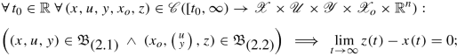  (2.4)

• (c) an asymptotic observer for(2.1), if it is an observer and a state estimator for (2.1).

The property of being a state estimator is much weaker than being an asymptotic observer. Since there is no requirement such as (2.3) it might even happen that the state estimator’s state matches the original system’s state for some time, but eventually evolves in a different direction.

Concluding this section we recall some important concepts for matrix pencils. First, a matrix pencil $sE-A \in \mathbb {R}[s]^{l \times n}$ is called regular, if l = n and $\det (sE-A) \neq 0 \in \mathbb {R}[s]$. An important geometric tool are the Wong sequences, named after Wong [39], who was the first to use both sequences for the analysis of matrix pencils. The Wong sequences are investigated and utilized for the decomposition of matrix pencils in [8,9,10].

Definition 2.4

Consider a matrix pencil $sE-A \in \mathbb {R}[s]^{l \times n}$. The Wong sequences are sequences of subspaces, defined by

$$\displaystyle \begin{aligned} \begin{array}{l l l} \mathcal{V}_{[E,A]}^0 := \mathbb{R}^n, & \mathcal{V}_{[E,A]}^{i+1} := A^{-1}(E \mathcal{V}_{[E,A]}^i) \subseteq \mathbb{R}^n, & \mathcal{V}_{[E,A]}^* := \bigcap\limits_{i \in \mathbb{N}_0}\mathcal{V}_{[E,A]}^i,\\ \mathcal{W}_{[E,A]}^0 := \{0\}, & \mathcal{W}_{[E,A]}^{i+1} := E^{-1}(A\mathcal{W}_{[E,A]}^i) \subseteq \mathbb{R}^n, & \mathcal{W}_{[E,A]}^* := \bigcup\limits_{i \in \mathbb{N}_0}\mathcal{W}_{[E,A]}^i, \end{array} \end{aligned}$$

where $A^{-1}(S) = \{ x \in \mathbb {R}^n \mid Ax \in S \}$ is the preimage of $S \subseteq \mathbb {R}^l$ under A. The subspaces $\mathcal {V}_{[E,A]}^*$ and $\mathcal {W}_{[E,A]}^*$ are called the Wong limits .

As shown in [8] the Wong sequences terminate, are nested and satisfy

$$\displaystyle \begin{aligned} &\exists\, k^* \in \mathbb{N}\,\, \forall j \in \mathbb{N} : \mathcal{V}_{[E,A]}^0 \supsetneq \mathcal{V}_{[E,A]}^1 \supsetneq \dots \supsetneq \mathcal{V}_{[E,A]}^{k^*} = \mathcal{V}_{[E,A]}^{k^*+j} = \mathcal{V}_{[E,A]}^{*} \supseteq \ker(A), \\ &\exists\, l^* \in \mathbb{N} \,\, \forall j \in \mathbb{N} : \mathcal{W}_{[E,A]}^0 \subseteq \ker(E) = \mathcal{W}_{[E,A]}^1 \subsetneq \dots \subsetneq \mathcal{W}_{[E,A]}^{l^*} = \mathcal{W}_{[E,A]}^{l^*+j} = \mathcal{W}_{[E,A]}^{*}. \end{aligned}$$

Remark 2.1

Let $sE-A \in \mathbb {R}[s]^{l \times n}$ and consider the associated DAE $\tfrac {\text{ d}}{\text{ d}t} E x(t) = Ax(t)$. In view of Definition 2.1 we may associate with the previous equation the behavior

We have that all trajectories in $\mathfrak {B}_{[E,A]}$ evolve in $\mathcal {V}_{[E,A]}^{*}$, that is

$$\displaystyle \begin{aligned} \forall\, x \in \mathfrak{B}_{[E,A]} \ \ \forall\, t \in \operatorname{\mathrm{\mathrm{dom}}}(x): \ \ x(t) \in \mathcal{V}_{[E,A]}^{*}. \end{aligned} $$

(2.5)

This can be seen as follows: For $x \in \mathfrak {B}_{[E,A]}$ we have that $x(t) \in \mathbb {R}^n = \mathcal {V}_{[E,A]}^0$ for all $t \in \operatorname {\mathrm {\mathrm {dom}}}(x)$. Since the linear spaces $\mathcal {V}_{[E,A]}^i$ are closed they are invariant under differentiation and hence $\dot {x}(t) \in \mathcal {V}_{[E,A]}^0$. Due to the fact that $x \in \mathfrak {B}_{[E,A]}$ it follows for all $t \in \operatorname {\mathrm {\mathrm {dom}}}(x)$ that $x(t) \in A^{-1} (E\mathcal {V}_{[E,A]}^0) = \mathcal {V}_{[E,A]}^1$. Now assume that $x(t) \in \mathcal {V}_{[E,A]}^i$ for some $i \in \mathbb {N}_0$ and all $t\in \operatorname {\mathrm {\mathrm {dom}}}(x)$. By the previous arguments we find that $x(t) \in A^{-1}(E\mathcal {V}_{[E,A]}^i) = \mathcal {V}_{[E,A]}^{i+1}$.

An important concept in the context of DAEs is the index of a matrix pencil, which is based on the (quasi-)Weierstraß form (QWF), cf. [10, 18, 24, 25].

Definition 2.5

Consider a regular matrix pencil $sE-A \in \mathbb {R}[s]^{n \times n}$ and let $S,T\in {\mathbb {R}}^{n\times n}$ be invertible such that

for some $J\in {\mathbb {R}}^{r\times r}$ and nilpotent $N\in {\mathbb {R}}^{(n-r)\times (n-r)}$. Then

is called the index of sE − A.

The index is independent of the choice of S, T and can be computed via the Wong sequences as shown in [10].

3 System, Observer Candidate and Error Dynamics

In this section we present the observer design used in this paper, which invokes so called innovations and was developed in [34, 37] for linear behavioral systems. It is an extension of the classical approach to observer design which goes back to Luenberger, see [30, 31].

We consider nonlinear DAE systems of the form

$$\displaystyle \begin{aligned} \tfrac{\text{ d}}{\text{ d}t} E x(t) &= Ax(t) + B_L f_L(x(t),u(t),y(t)) + B_M f_M(Jx(t),u(t),y(t)),\\ y(t) &= Cx(t) + h(u(t)), \end{aligned} $$

(3.1)

where $E,A \in \mathbb {R}^{l \times n}$ with $0\leq r= \operatorname {\mathrm {rk}}(E)\leq n$, $B_L \in \mathbb {R}^{l \times q_L}$, $B_M \in \mathbb {R}^{l \times q_M}$, $J \in \mathbb {R}^{q_M \times n}$ with $\operatorname {\mathrm {rk}} J =~q_M$, $C \in \mathbb {R}^{p \times n}$ and $h \in \mathcal {C}(\mathcal {U} \to \mathbb {R}^p)$ with $\mathcal {U} \subseteq \mathbb {R}^m$ open. Furthermore, for some open sets $\mathcal {X} \subseteq \mathbb {R}^n, \mathcal {Y} \subseteq \mathbb {R}^p$ and $\hat {\mathcal {X}} := J \mathcal {X} \subseteq {\mathbb {R}}^{q_M}$, the nonlinear function $f_L:\mathcal {X} \times \mathcal {U} \times \mathcal {Y} \to \mathbb {R}^{q_{L}}$ satisfies a Lipschitz condition in the first variable

$$\displaystyle \begin{aligned} \forall\, x,z \in \mathcal{X}\ \forall\, u \in \mathcal{U}\ \forall\, y \in \mathcal{Y}: \ \ \|f_L(z,u,y)-f_L(x,u,y)\| \leq \|F(z-x)\| \end{aligned} $$

(3.2)

with $F \in \mathbb {R}^{j \times n}$, $j \in \mathbb {N}$; and $f_M: \hat {\mathcal {X}} \times \mathcal {U} \times \mathcal {Y} \to \mathbb {R}^{q_{M}}$ satisfies a generalized monotonicity condition in the first variable

$$\displaystyle \begin{aligned} \forall\, x,z \in \hat{\mathcal{X}}\ \forall\, u \in \mathcal{U}\ \forall\, y \in \mathcal{Y}: \ \ (z-x)^\top \varTheta \big( f_M(z,u,y)-f_M(x,u,y) \big) \geq \frac{1}{2}\mu \|z-x\|{}^2 \end{aligned} $$

(3.3)

for some $\varTheta \in \mathbb {R}^{q_M \times q_M}$ and $\mu \in \mathbb {R}$. We stress that μ < 0 is explicitly allowed and Θ can be singular, i.e., in particular Θ does not necessarily satisfy any definiteness conditions as in [40]. We set $B := [B_L, B_M] \in \mathbb {R}^{l \times (q_L + q_M)}$ and

$$\displaystyle \begin{aligned} f : \mathcal{X} \times \mathcal{U} \times \mathcal{Y} \to \mathbb{R}^{q_{L}} \times \mathbb{R}^{q_M},\ (x,u,y) \mapsto \begin{pmatrix} f_L(x,u,y) \\ f_M(Jx,u,y) \end{pmatrix}. \end{aligned}$$

Let us consider a system (3.1) and assume that n = l. Then another system driven by the external variables u and y of (3.1) of the form

$$\displaystyle \begin{aligned} \tfrac{\text{ d}}{\text{ d}t} E z(t) &= Az(t) + Bf(z(t),u(t),y(t)) + L(y(t)-\hat{y}(t)) \\ &= Az(t) + Bf(z(t),u(t),y(t)) + L(Cx(t)-Cz(t)) \\ &= (A-LC)z(t) + Bf(z(t),u(t),y(t)) + L \underbrace{Cx(t)}_{= y(t) - h(u(t))} \\ \text{with} \ \ \hat{y}(t) &= C z(t) + h(u(t)) \end{aligned} $$

(3.4)

is a Luenberger type observer , where $L\in {\mathbb {R}}^{n\times p}$ is the observer gain. The dynamics for the error state e(t) = z(t) − x(t) read

$$\displaystyle \begin{aligned} \tfrac{\text{ d}}{\text{ d}t} E e(t) = (A-LC)e(t) + B\big(f(x(t),u(t),y(t))-f(z(t),u(t),y(t))\big). \end{aligned}$$

The observer (3.4) incorporates a copy of the original system, and in addition the outputs’ difference $\hat {y}(t)-y(t)$, the influence of which is weighted with the observer gain L.

In this paper we consider a generalization of the design (3.4) which incorporates an extra variable d that takes the role of the innovations . The innovations are used to describe “the difference between what we actually observe and what we had expected to observe” [34], and hence they generalize the effect of the observer gain L in (3.4). We consider the following observer candidate, which is an additive composition of an internal model of the system (3.1) and a further term which involves the innovations:

$$\displaystyle \begin{aligned} \tfrac{\text{ d}}{\text{ d}t} Ez(t)&=Az(t)+Bf(z(t),u(t),y(t))+L_1 d(t) \\ 0&=Cz(t)-y(t)+h(u(t))+L_2 d(t), \end{aligned} $$

(3.5)

where is the observer state and $L_1 \in \mathbb {R}^{l \times k}$, $L_2 \in \mathbb {R}^{p \times k}$, $\mathcal {X}_o = \mathcal {X} \times \mathbb {R}^k$. From the second line in (3.5) we see that the innovations term balances the difference between the system’s and the observer’s output. In a sense, the smaller the variable d, the better the approximate state z in (3.5) matches the state x of the original system (3.1).

We stress that n ≠ l is possible in general, and if L ₂ is invertible, then the observer candidate reduces to

$$\displaystyle \begin{aligned} \tfrac{\text{ d}}{\text{ d}t} E {z}(t) &= Az(t) + Bf(z(t),u(t),y(t))+L_1 L_2^{-1}(y(t) - Cz(t) - h(u(t))) \\ &= (A - L_1 L_2^{-1} C)z(t) + Bf(z(t),u(t),y(t)) + L_1 L_2^{-1}(\underbrace{y(t) - h(u(t))}_{=Cx(t)}), \end{aligned} $$

(3.6)

which is a Luenberger type observer of the form (3.4) with gain $L=L_1 L_2^{-1}$. Hence the Luenberger type observer is a special case of the observer design (3.5). Being square is a necessary condition for invertibility of L ₂, i.e., k = p.

For later use we consider the dynamics of the error state e(t):= z(t) − x(t) between systems (3.1) and (3.5),

$$\displaystyle \begin{aligned} \tfrac{\text{ d}}{\text{ d}t} Ee(t) &=Ae(t)+B\phi(t) +L_1d(t) \\ 0&=Ce(t)+L_2d(t), \end{aligned} $$

(3.7)

where

and rewrite (3.7) as

(3.8)

where

$$\displaystyle \begin{aligned} & \mathcal{E} = \begin{bmatrix} E & 0 \\ 0 & 0 \end{bmatrix} \in \mathbb{R}^{(l+p) \times (n+k)},\quad \mathcal{A} = \begin{bmatrix} A & L_1 \\ C & L_2 \end{bmatrix} \in \mathbb{R}^{(l+p) \times (n+k)}\\ and\quad & \mathcal{B} = \begin{bmatrix} B \\ 0 \end{bmatrix} \in \mathbb{R}^{(l+p) \times (q_L + q_M)}. \end{aligned} $$

The following lemma is a consequence of (2.5).

Lemma 3.1

Consider a system (3.1) and the observer candidate (3.5). Then (3.5) is an acceptor for (3.1). Furthermore, for all open intervals $I \subseteq \mathbb {R}$, all $(x,u,y) \in \mathfrak {B}_{\mathit{\mbox{{(3.1)}}}}$and all $\left (\binom {z}{d},\binom {u}{y},z \right ) \in \mathfrak {B}_{\mathit{\mbox{{(3.5)}}}}$with $\operatorname {\mathrm {\mathrm {dom}}}(x)= \operatorname {\mathrm {\mathrm {dom}}}\binom {z}{d} = I$we have:

(3.9)

Proof

Let $I \subseteq \mathbb {R}$ be an open interval and $(x,u,y) \in \mathfrak {B}_{\mbox{{(3.1)}}}$. For any $(x,u,y) \in \mathfrak {B}_{\mbox{{(3.1)}}}$ it holds $\left (\binom {x}{0},\binom {u}{y},x \right ) \in \mathfrak {B}_{\mbox{{(3.5)}}}$, hence (3.5) is an acceptor for (3.1).

Now let $(x,u,y) \in \mathfrak {B}_{\mbox{{(3.1)}}}$ and $\left (\binom {z}{d},\binom {u}{y},z \right ) \in \mathfrak {B}_{\mbox{{(3.5)}}}$, with $I= \operatorname {\mathrm {\mathrm {dom}}}(x)= \operatorname {\mathrm {\mathrm {dom}}}\binom {z}{d}$ and rewrite (3.8) as

Then (3.9) is immediate from Remark 2.1. □

In the following lemma we show that for a state estimator to exist, it is necessary that the system (3.1) does not contain free state variables, i.e., solutions (if they exist) are unique.

Lemma 3.2

Consider a system (3.1) and the observer candidate (3.5). If (3.5) is a state estimator for (3.1), then either

(3.10)

or we have .

Proof

Let (3.5) be a state estimator for (3.1) and assume that (3.10) is not true. Set , and let $(x,u,y)~\in ~\mathfrak {B}_{\mbox{{(3.1)}}}$ with $[t_0,\infty )\subseteq \operatorname {\mathrm {\mathrm {dom}}}(x)$ for some $t_0\in {\mathbb {R}}$. Then we have that, for all t ≥ t ₀,

$$\displaystyle \begin{aligned} \tfrac{\text{ d}}{\text{ d}t} E' x(t) = \begin{bmatrix} A \\ C \end{bmatrix} x(t) + \begin{bmatrix} B & L_1 \\ 0 & L_2 \end{bmatrix} \begin{pmatrix} f(x(t),u(t),y(t)) \\ d(t) \end{pmatrix} =: A' x(t) + g(x(t),u(t),y(t),d(t)) \end{aligned} $$

(3.11)

with d(t) ≡ 0. Using [8, Thm. 2.6] we find matrices $S \in Gl_{l+p}({\mathbb {R}})$, $T \in Gl_{n}({\mathbb {R}})$ such that

$$\displaystyle \begin{aligned} S\left(sE' - A'\right)T = s\begin{bmatrix} E_P & 0 & 0 \\ 0& E_R & 0 \\ 0& 0&E_Q \end{bmatrix} - \begin{bmatrix} A_P & 0 & 0 \\ 0& A_R & 0 \\ 0 & 0 & A_Q \end{bmatrix}, \end{aligned} $$

(3.12)

where

• (i) $E_P , A_P \in {\mathbb {R}}^{m_P \times n_P}, m_P < n_P$, are such that $\operatorname {\mathrm {rk}}_{{\mathbb {C}}}(\lambda E_P-A_P) = m_P$ for all $\lambda \in {\mathbb {C}} \cup \{ \infty \}$,

• (ii) $E_R , A_R \in {\mathbb {R}}^{m_R \times n_R}, m_R = n_R$, with sE _R − A _R regular,

• (iii) $E_Q , A_Q \in {\mathbb {R}}^{m_Q \times n_Q}, m_Q > n_Q$, are such that $\operatorname {\mathrm {rk}}_{{\mathbb {C}}}(\lambda E_Q-A_Q) = n_Q$ for all $\lambda \in {\mathbb {C}} \cup \{ \infty \}$.

We consider the underdetermined pencil sE _P − A _P in (3.12) and the corresponding DAE. If n _P = 0, then [8, Lem. 3.1] implies that $\operatorname {\mathrm {rk}}_{{\mathbb {R}}(s)} sE_Q-A_Q = n_Q$ and invoking $\operatorname {\mathrm {rk}}_{{\mathbb {R}}(s)} s E_R- A_R = n_R$ gives that $\operatorname {\mathrm {rk}}_{{\mathbb {R}}(s)} s E' -A' = n$. So assume that n _p > 0 in the following and set

$$\displaystyle \begin{aligned} \begin{pmatrix} x_p \\ x_R \\ x_Q \end{pmatrix} := T^{-1} x, \quad \begin{pmatrix} g_p \\ g_R \\ g_Q \end{pmatrix} := S g. \end{aligned}$$

If m _p = 0, then x _P can be chosen arbitrarily. Otherwise, we have

(3.13)

As a consequence of [8, Lem. 4.12] we may w.l.o.g. assume that $sE_P-A_P = s[I_{m_p},0]-[N,R]$ with $R\in {\mathbb {R}}^{m_P\times (n_P-m_P)}$ and nilpotent $N\in {\mathbb {R}}^{m_P\times m_P}$. Partition , then (3.13) is equivalent to

$$\displaystyle \begin{aligned} \dot{x}_P^1(t) = N x_P^1(t) + R x_P^2(t) + g_P\big( T(x_P^1(t)^\top, x_P^2(t)^\top, x_R(t)^\top, x_Q(t)^\top)^\top,u(t),y(t),d(t)\big) \end{aligned} $$

(3.14)

for all t ≥ t ₀, and hence $x_P^2\in \mathcal {C}([t_0,\infty )\to {\mathbb {R}}^{n_P-m_P})$ can be chosen arbitrarily and every choice preserves $[t_0,\infty )\subseteq \operatorname {\mathrm {\mathrm {dom}}}(x)$. Similarly, if with $[t_0,\infty )\subseteq \operatorname {\mathrm {\mathrm {dom}}}(z)$—w.l.o.g. the same t ₀ can be chosen—then (3.11) is satisfied for x = z and, proceeding in an analogous way, $z_P^2$ can be chosen arbitrarily, in particular such that $\lim _{t \to \infty }~z_P^2(t)~\neq ~\lim _{t \to \infty }~x_P^2(t)$. Therefore, lim_t→∞z(t)  − x(t)  =  lim_t→∞e(t)  ≠  0, which contradicts that (3.5) is a state estimator for (3.1). Thus n _P = 0 and $\operatorname {\mathrm {rk}}_{{\mathbb {R}}(s)} s E' -A' = n$ follows. □

As a consequence of Lemma 3.2, a necessary condition for (3.5) to be a state estimator for (3.1) is that n ≤ l + p. This will serve as a standing assumption in the subsequent sections.

4 Sufficient Conditions for State Estimators

In this section we show that if certain matrix inequalities are satisfied, then there exists a state estimator for system (3.1) which is of the form (3.5). The design parameters of the latter can be obtained from a solution of the matrix inequalities. The proofs of the subsequent theorems are inspired by the work of Lu and Ho [29] and by [5], where LMIs are considered on the Wong limits only.

Theorem 4.1

Consider a system (3.1) with n ≤ l + p which satisfies conditions (3.2) and (3.3). Let $k \in {\mathbb {N}}_0$and denote with $\mathcal {V}^*_{\left [[\mathcal {E}, 0], [\mathcal {A}, \mathcal {B}] \right ]}$the Wong limit of the pencil $s[\mathcal {E},0]-[\mathcal {A},\mathcal {B}] \in \mathbb {R}[s]^{(l+p)\times (n+k+q_L+q_M)}$, and $\overline {\mathcal {V}}^*_{\left [[\mathcal {E}, 0], [\mathcal {A}, \mathcal {B}] \right ]}~:=~\left [I_{n+k}, 0 \right ] \mathcal {V}^*_{\left [[\mathcal {E}, 0], [\mathcal {A}, \mathcal {B}] \right ]}$. Further let , , $\mathcal {F}~=~[ F , 0]~\in \mathbb {R}^{j \times (n+k)}$, $j~\in ~\mathbb {N}$, $\hat {\varTheta }~=~\begin {bmatrix}0& J^\top \varTheta \\0& 0 \end {bmatrix}~\in ~\mathbb {R}^{(n+k) \times (q_L+q_M)}$, $\mathcal {J}~=~\begin {bmatrix} J^\top J & 0 \\0 & 0 \end {bmatrix}~\in ~\mathbb {R}^{(n+k) \times (n+k)}$and $\varLambda _{q_L}~:=~\begin {bmatrix} I_{q_L} & 0 \\0 & 0 \end {bmatrix}~\in ~\mathbb {R}^{(q_L+q_M) \times (q_L+q_M)}$.

If there exist δ > 0, $\mathcal {P}~\in ~\mathbb {R}^{(l+p) \times (n+k)}$and $\mathcal {K}~\in ~\mathbb {R}^{(n+k) \times (n+k)}$such that

$$\displaystyle \begin{aligned} \mathcal{Q} := \begin{bmatrix} \hat{A}^\top\mathcal{P} + \mathcal{P}^\top \hat{A} + H^\top \mathcal{K}^\top + \mathcal{K}H+ \delta \mathcal{F}^\top \mathcal{F} -\mu \mathcal{J} & \mathcal{P}^\top\mathcal{B}+\hat{\varTheta} \\ \mathcal{B}^\top\mathcal{P}+\hat{\varTheta}^\top & -\delta \varLambda_{q_L} \end{bmatrix} <_{\mathcal{V}^*_{\left[[\mathcal{E}, 0], [\mathcal{A}, \mathcal{B}] \right]}} 0 \end{aligned} $$

(4.1)

and

$$\displaystyle \begin{aligned} \mathcal{P}^\top \mathcal{E} = \mathcal{E}^\top \mathcal{P} >_{\overline{\mathcal{V}}^*_{\left[[\mathcal{E}, 0], [\mathcal{A}, \mathcal{B}] \right]}} 0, \end{aligned} $$

(4.2)

then for all $L_1 \in \mathbb {R}^{l\times k}$, $L_2 \in \mathbb {R}^{p \times k}$such that the system (3.5) is a state estimator for (3.1).

Furthermore, there exists at least one such pair L ₁, L ₂if, and only if, $\operatorname {\mathrm {im}} \mathcal {K} H \subseteq \operatorname {\mathrm {im}} \mathcal {P}^\top$.

Proof

Using Lemma 3.1, we have that (3.5) is an acceptor for (3.1). To show that (3.5) satisfies condition (2.4) let $t_0 \in \mathbb {R}$ and $(x,u,y,x_o,z) \in \mathcal {C}([t_0,\infty ) \to \mathcal {X} \times \mathcal {U} \times \mathcal {Y} \times \mathcal {X}_o \times \mathbb {R}^n)$ such that $(x,u,y) \in \mathfrak {B}_{\mbox{{(3.1)}}}$ and $(x_o,\binom {u}{y},z) \in \mathfrak {B}_{\mbox{{(3.5)}}}$, with $x_o(t) = \binom {z(t)}{d(t)}$ and $\mathcal {X}_o = \mathcal {X} \times \mathbb {R}^k$.

The last statement of the theorem is clear. Let $\hat {L} = [0_{(l+p)\times n}, \ast ]$ be a solution of $\mathcal {P}^\top \hat {L}~=~\mathcal {K} H$ and $\mathcal {A}~=~\hat {A}~+~\hat {L}$, further set , where e(t)  =  z(t)  − x(t). Recall that

$$\displaystyle \begin{aligned} \phi(t) &= f(z(t),u(t),y(t))-f(x(t),u(t),y(t)) \\ &= \begin{pmatrix} f_L(z(t),u(t),y(t))-f_L(x(t),u(t),y(t))\\ f_M(Jz(t),u(t),y(t))-f_M(Jx(t),u(t),y(t))\end{pmatrix} =: \begin{pmatrix} \phi_L(t)\\ \phi_M(t)\end{pmatrix}. \end{aligned} $$

In view of condition (3.2) we have for all t ≥ t ₀ that

$$\displaystyle \begin{aligned} \delta (\eta^\top(t) \mathcal{F}^\top\mathcal{F} \eta(t) - \phi_L^\top(t) \phi_L(t)) \geq 0 \end{aligned} $$

(4.3)

and by (3.3)

$$\displaystyle \begin{aligned} ([J,0]\eta(t))^\top \varTheta \phi_M(t) + \phi_M^\top (t) \varTheta^\top [J,0]\eta(t) - \mu ([J,0]\eta(t))^\top ([J,0]\eta(t)) \geq 0. \end{aligned} $$

(4.4)

Now assume that (4.1) and (4.2) hold. Consider a Lyapunov function candidate

$$\displaystyle \begin{aligned} \tilde{V} \colon \mathbb{R}^{n+k} \to \mathbb{R}, \ \ \eta \mapsto \eta^\top \mathcal{E}^\top \mathcal{P} \eta \end{aligned}$$

and calculate the derivative along solutions for t ≥ t ₀:

$$\displaystyle \begin{aligned} \tfrac{\text{ d}}{\text{ d}t}\tilde{V}(\eta(t)) &= \dot{\eta}^\top(t) \mathcal{E}^\top \mathcal{P} \eta(t) + \eta^\top(t) \mathcal{P}^\top \mathcal{E} \dot{\eta}(t) \\ &=\left(\mathcal{A}\eta(t) + \mathcal{B}\phi(t) \right)^\top \mathcal{P} \eta(t) + \eta^\top(t) \mathcal{P}^\top \left(\mathcal{A}\eta(t) + \mathcal{B}\phi(t) \right) \\ &= \eta^\top(t) \mathcal{A}^\top\mathcal{P}\eta(t) + \eta^\top(t) \mathcal{P}^\top\mathcal{A}\eta(t) + \phi^\top(t) \mathcal{B}^\top\mathcal{P}\eta(t) + \eta^\top(t) \mathcal{P}^\top\mathcal{B}\phi(t) \\ &= \eta^\top(t) \hat{A}^\top \mathcal{P} \eta(t) + \eta^\top(t) \hat{L}^\top \mathcal{P} \eta(t) + \eta^\top(t) \mathcal{P}^\top \hat{A} \eta(t) + \eta^\top(t) \mathcal{P}^\top \hat{L} \eta(t) \\ &\ \ \ \ \ + \phi^\top(t) \mathcal{B}^\top\mathcal{P}\eta(t) + \eta^\top(t) \mathcal{P}^\top\mathcal{B}\phi(t) \\ & \overset{(4.3),(4.4)}{\leq} \eta^\top(t) \left( \hat{A}^\top \mathcal{P} + \mathcal{P}^\top \hat{A} + \mathcal{K} H + H^\top \mathcal{K}^\top \right) \eta(t)\\ &\ \ \ \ \ + \phi^\top(t) \mathcal{B}^\top\mathcal{P}\eta(t) + \eta^\top(t) \mathcal{P}^\top\mathcal{B}\phi(t) + \delta (\eta^\top(t) \mathcal{F}^\top\mathcal{F} \eta(t) - \phi_L^\top(t) \phi_L(t)) \\ &\ \ \ \ \ + ([J,0]\eta(t))^\top \varTheta \phi_M(t) + \phi_M^\top (t) \varTheta^\top [J,0]\eta(t) - \mu ([J,0]\eta(t))^\top ([J,0]\eta(t)) \\ &= \eta^\top(t) \left( \hat{A}^\top \mathcal{P} + \mathcal{P}^\top \hat{A} + \mathcal{K} H + H^\top \mathcal{K}^\top + \delta \mathcal{F}^\top\mathcal{F}-\mu \mathcal{J} \right) \eta(t)\\ &\ \ \ \ \ + \phi^\top(t) \mathcal{B}^\top\mathcal{P}\eta(t) + \eta^\top(t) \mathcal{P}^\top\mathcal{B}\phi(t) \\ &\ \ \ \ \ + \eta^\top(t) \hat{\varTheta} \phi(t) + \phi^\top (t) \hat{\varTheta}^\top \eta(t) - \delta \phi^\top(t) \varLambda_{q_L} \phi(t)\\ = \begin{pmatrix} \eta(t) \\ \phi(t)\end{pmatrix}^\top &\underset{=\mathcal{Q}}{\underbrace{\begin{bmatrix} \hat{A}^\top\mathcal{P} + \mathcal{P}^\top\hat{A} + H^\top \mathcal{K}^\top + \mathcal{K}H+ \delta \mathcal{F}^\top\mathcal{F}-\mu \mathcal{J} & \mathcal{P}^\top\mathcal{B}+\hat{\varTheta} \\ \mathcal{B}^\top\mathcal{P}+\hat{\varTheta}^\top & -\delta \varLambda_{q_L} \end{bmatrix}}} \begin{pmatrix} \eta(t) \\ \phi(t)\end{pmatrix}.{} \end{aligned} $$

(4.5)

Let $S \in \mathbb {R}^{(n+k+q_L+q_M) \times n_{\mathcal {V}}}$ with orthonormal columns be such that $\operatorname {\mathrm {im}} S=\mathcal {V}^*_{\left [[\mathcal {E}, 0], [\mathcal {A}, \mathcal {B}] \right ]}$ and $\operatorname {\mathrm {rk}}(S)=n_{\mathcal {V}}$. Then inequality (4.1) reads $\hat {\mathcal {Q}}:=S^\top \mathcal {Q} S < 0$. Denote with $\lambda _{\hat {\mathcal {Q}}}^-$ the smallest eigenvalue of $-\hat {\mathcal {Q}}$, then $\lambda _{\hat {\mathcal {Q}}}^- >0$. Since S has orthonormal columns we have ∥Sv∥  =  ∥v∥ for all $v~\in ~\mathbb {R}^{n_{\mathcal {V}}}$.

By Lemma 3.1 we have for all t ≥ t ₀, hence for some $v\colon [t_0, \infty ) \to \mathbb {R}^{n_{\mathcal {V}}}$. Then (4.5) becomes

$$\displaystyle \begin{aligned} \forall\, t \geq t_0:\,\tfrac{\text{ d}}{\text{ d}t} \tilde{V}(\eta(t)) &\leq \begin{pmatrix} \eta(t) \\ \phi(t) \end{pmatrix}^\top \mathcal{Q} \begin{pmatrix} \eta(t) \\ \phi(t) \end{pmatrix} = v^\top(t) \hat{\mathcal{Q}} v(t) \\ & \leq - \lambda_{\hat{\mathcal{Q}}}^- \|v(t)\|{}^2 = - \lambda_{\hat{\mathcal{Q}}}^- \left\|\begin{pmatrix} \eta(t) \\ \phi(t)\end{pmatrix}\right\|{}^2. \end{aligned} $$

(4.6)

Let $\overline {S} \in \mathbb {R}^{(n+k)\times n_{\overline {\mathcal {V}}}}$ with orthonormal columns be such that $\operatorname {\mathrm {im}} \overline {S} =\overline {\mathcal {V}}^*_{\left [[\mathcal {E}, 0], [\mathcal {A}, \mathcal {B}] \right ]}$ and $\operatorname {\mathrm {rk}}(\overline {S})= n_{\overline {\mathcal {V}}}$. Then condition (4.2) is equivalent to $\overline {S}^\top \mathcal {E}^\top \mathcal {P} \overline {S}>0$. Since for all t ≥ t ₀ it is clear that $\eta (t) \in \overline {\mathcal {V}}^*_{\left [[\mathcal {E}, 0], [\mathcal {A}, \mathcal {B}] \right ]}$ for all t ≥ t ₀. If $\overline {\mathcal {V}}^*_{\left [[\mathcal {E}, 0], [\mathcal {A}, \mathcal {B}] \right ]} = \{0\}$ (which also holds when ${\mathcal {V}}^*_{\left [[\mathcal {E}, 0], [\mathcal {A}, \mathcal {B}] \right ]}=\{0\}$), then this implies η(t) = 0, thus e(t) = 0 for all t ≥ t ₀, which completes the proof. Otherwise, $n_{\overline {\mathcal {V}}} > 0$ and we set $\eta (t) = \overline {S} \bar {\eta }(t)$ for some $\bar {\eta }\colon [t_0, \infty )\to \mathbb {R}^{n_{\overline {\mathcal {V}}}}$ and denote with λ ⁺, λ ⁻ the largest and smallest eigenvalue of $\overline {S}^\top \mathcal {E}^\top \mathcal {P} \overline {S}$, resp., where λ ⁻ > 0 is a consequence of (4.2). Then we have

$$\displaystyle \begin{aligned} \tilde{V}(\eta(t)) = \eta^\top(t) \mathcal{E}^\top\mathcal{P} \eta(t) = \bar{\eta}^\top(t) \overline{S}^\top\mathcal{E}^\top\mathcal{P}\overline{S}\bar{\eta}(t) \leq \lambda^+ \|\bar{\eta}(t)\|{}^2 = \lambda^+ \|\eta(t)\|{}^2 \end{aligned} $$

(4.7)

and, analogously,

$$\displaystyle \begin{aligned} \forall\, t \geq t_0:\, \lambda^- \|\eta(t)\|{}^2 \leq \bar{\eta}^\top(t)\overline{S}^\top \mathcal{E}^\top\mathcal{P} \overline{S}\bar{\eta}(t) = \tilde{V}(\eta(t)) \leq \lambda^+ \|\eta(t)\|{}^2. \end{aligned} $$

(4.8)

Therefore,

$$\displaystyle \begin{aligned} \forall\, t \geq t_0 : \, \tfrac{\text{ d}}{\text{ d}t} \tilde{V}(\eta(t)) \overset{(\text{4.6})}{\leq} -\lambda_{\hat{\mathcal{Q}}}^- \left\|\begin{pmatrix} \eta(t) \\ \phi(t)\end{pmatrix}\right\|{}^2 \leq -\lambda_{\hat{\mathcal{Q}}}^- \|\eta(t)\|{}^2 \overset{(\text{4.7})}{\leq} -\frac{\lambda_{\hat{\mathcal{Q}}}^-}{\lambda^+} \,\, \tilde{V}(\eta(t)). \end{aligned}$$

Now, abbreviate $\beta := \frac {\lambda _{\hat {\mathcal {Q}}}^-}{\lambda ^+}$ and use Gronwall’s Lemma to infer

$$\displaystyle \begin{aligned} \forall\, t \geq t_0:\, \tilde{V}(\eta(t)) \leq \tilde{V}(\eta(0)) e^{-\beta t}. \end{aligned} $$

(4.9)

Then we obtain

$$\displaystyle \begin{aligned} \forall\, t\ge t_0:\ \|\eta(t)\|{}^2 \stackrel{(4.8)}{\leq} \frac{1}{\lambda^-} \tilde{V}(\eta(t)) \overset{(4.9)}{\leq} \frac{\tilde{V}(\eta(0))}{\lambda^-} e^{-\beta t}, \end{aligned}$$

and hence lim_t→∞e(t) = 0, which completes the proof. □

Remark 4.1

• (i) Note that $\mathcal {A} = \hat A + \hat {L}$, where $\hat {L} = [0_{(l+p)\times n}, \ast ]$ is a solution of $\mathcal {P}^\top \hat {L} = \mathcal {K} H$ and hence the space ${\mathcal {V}_{\left [[\mathcal {E},0],[\mathcal {A},\mathcal {B}] \right ]}^*}$ on which (4.1) is considered depends on the sought solutions $\mathcal {P}$ and $\mathcal {K}$ as well; using $\mathcal {P}^\top \mathcal {A} = \mathcal {P}^\top \hat A + \mathcal {K} H$, this dependence is still linear. Furthermore, note that $\mathcal {K}$ only appears in union with the matrix , thus only the last k columns of $\mathcal {K}$ are of interest. In order to reduce the computational effort it is reasonable to fix the other entries beforehand, e.g. by setting them to zero.

• (ii) We stress that the parameters in the description (3.1) of the system are not entirely fixed, especially regarding the linear parts. More precisely, an equation of the form $\tfrac {\text{ d}}{\text{ d}t} E x(t) = Ax(t) + f(x(t),u(t))$, where f satisfies (3.2) can equivalently be written as $\tfrac {\text{ d}}{\text{ d}t} E x(t) = f_L(x(t),u(t))$, where f _L(x, u) = Ax + f(x, u) also satisfies (3.2), but with a different matrix F. However, this alternative (with A = 0) may not satisfy the necessary condition provided in Lemma 3.2, which hence should be checked in advance. Therefore, the system class (3.1) allows for a certain flexibility and different choices of the parameters may or may not satisfy the assumptions of Theorem 4.1.

• (iii) In the special case E = 0, i.e., purely algebraic systems of the form 0 = Ax(t) + Bf(x(t), u(t), y(t)), Theorem 4.1 may still be applicable. More precisely, condition (4.2) is satisfied in this case if, and only if, $\overline {\mathcal {V}}^*_{\left [[\mathcal {E}, 0], [\mathcal {A}, \mathcal {B}] \right ]} = \{0\}$. This can be true, if for instance $\mathcal {B}=0$ and $\mathcal {A}$ has full column rank, because then $\overline {\mathcal {V}}^*_{\left [[\mathcal {E}, 0], [\mathcal {A}, \mathcal {B}] \right ]} = [I_{n+k}, 0] \ker [\mathcal {A}, 0] = \{0\}$.

In the following theorem condition (4.2) is weakened to positive semi-definiteness. As a consequence, the system’s matrices have to satisfy additional conditions, which are not present in Theorem 4.1. In particular, we require that $\mathcal {E}$ and $\mathcal {A}$ are square, which means that k  =  l + p − n. Furthermore, we require that JG _M is invertible for a certain matrix G _M and that the norms corresponding to F and J are compatible if both kinds of nonlinearities are present.

Theorem 4.2

Use the notation from Theorem 4.1and set k = l + p − n. In addition, denote with $\mathcal {V}^*_{[\mathcal {E},\mathcal {A}]}, \mathcal {W}^*_{[\mathcal {E},\mathcal {A}]} \subseteq \mathbb {R}^{n+k}$the Wong limits of the pencil $s\mathcal {E}-\mathcal {A} \in \mathbb {R}[s]^{(l+p)\times (n+k)}$and let $V\in \mathbb {R}^{(n+k) \times n_{\mathcal {V}}}$and $W \in \mathbb {R}^{(n+k) \times n_{\mathcal {W}}}$be basis matrices of $\mathcal {V}^*_{[\mathcal {E},\mathcal {A}]}$and $\mathcal {W}^*_{[\mathcal {E},\mathcal {A}]}$, resp., where $n_{\mathcal {V}}=\dim (\mathcal {V}^*_{[\mathcal {E},\mathcal {A}]})$and $n_{\mathcal {W}}=\dim (\mathcal {W}^*_{[\mathcal {E},\mathcal {A}]})$. Furthermore, denote with λ _max(M) the largest eigenvalue of a matrix M.

If there exist δ > 0, $\mathcal {P} \in \mathbb {R}^{(l+p) \times (n+k)}$invertible and $\mathcal {K} \in \mathbb {R}^{(n+k) \times (n+k)}$such that (4.1) holds and

(4.10)

then with $L_1 \in \mathbb {R}^{l\times k}$, $L_2 \in \mathbb {R}^{p \times k}$such that the system (3.5) is a state estimator for (3.1).

Proof

Assume (4.1) and (4.10) (a)–(e) hold. Up to Eq. (4.9) the proof remains the same as for Theorem 4.1. By (4.10) (b) we may infer from [10, Thm. 2.6] that there exist invertible $\mathcal {M} = \left [M_1^\top , M_2^\top \right ]^\top \in \mathbb {R}^{(n+k)\times (l+p)}$ with $M_1 \in \mathbb {R}^{r \times (l+p)}$, $M_2 \in \mathbb {R}^{(n+k-r) \times (l+p)}$ and invertible $\mathcal {N} = \left [N_1 , N_2 \right ] \in \mathbb {R}^{(n+k)\times (l+p)}$ with $N_1 \in \mathbb {R}^{(n+k) \times r}$, $N_2 \in \mathbb {R}^{(n+k) \times (l+p-r)}$ such that

$$\displaystyle \begin{aligned} \mathcal{M}(\mathcal{E}-\mathcal{A})\mathcal{N} = \begin{bmatrix} I_r - A_r & 0 \\ 0 & -I_{n+k-r} \end{bmatrix}, \end{aligned} $$

(4.11)

where $r= \operatorname {\mathrm {rk}}(\mathcal {E})$ and $A_r \in \mathbb {R}^{r \times r}$, and that

$$\displaystyle \begin{aligned} \mathcal{N} = [V, W],\quad \mathcal{M} = [\mathcal{E}V, \mathcal{A}W]^{-1}. \end{aligned} $$

(4.12)

Let

$$\displaystyle \begin{aligned} \mathcal{P} = \mathcal{M}^\top \begin{bmatrix} P_1 & P_2 \\ P_3 & P_4 \end{bmatrix} \mathcal{N}^{-1} \end{aligned} $$

(4.13)

with $P_1 \in \mathbb {R}^{n_{\mathcal {V}} \times n_{\mathcal {V}}}$, $P_4 \in \mathbb {R}^{n_{\mathcal {W}}\times n_{\mathcal {W}}}$ and $P_2, P_3^\top \in \mathbb {R}^{n_{\mathcal {V}} \times n_{\mathcal {W}}}$. Then condition (4.10) (a) implies P ₁ > 0 as follows. First, calculate

$$\displaystyle \begin{aligned} \mathcal{E}^\top\mathcal{P} &= \mathcal{N}^{-T} \begin{bmatrix} I_r & 0 \\ 0 & 0 \end{bmatrix} \mathcal{M}^{-T} \mathcal{M}^{T} \begin{bmatrix} P_1 & P_2 \\ P_3 & P_4 \end{bmatrix} \mathcal{N}^{-1} = \mathcal{N}^{-T} \begin{bmatrix} P_1 & P_2 \\ 0 & 0 \end{bmatrix} \mathcal{N}^{-1} \\ \end{aligned} $$

(4.14)

which gives P ₂ = 0 as $\mathcal {P}^\top \mathcal {E}=\mathcal {E}^\top \mathcal {P}$. Note that therefore P ₁ and P ₄ in (4.13) are invertible since $\mathcal {P}$ is invertible by assumption. By (4.14) we have

$$\displaystyle \begin{aligned} \mathcal{E}^\top\mathcal{P} & = \mathcal{N}^{-T} \begin{bmatrix} P_1 & 0 \\ 0 & 0 \end{bmatrix} \mathcal{N}^{-1} = [V, W]^{-T} \begin{bmatrix} P_1 & 0 \\ 0 & 0 \end{bmatrix} [V, W]^{-1}. \end{aligned} $$

(4.15)

It remains to show P ₁ ≥ 0. Next, we prove the inclusion

$$\displaystyle \begin{aligned} \mathcal{V}^*_{[\mathcal{E},\mathcal{A}]} \subseteq \overline{\mathcal{V}}^*_{\left[[\mathcal{E},0],[\mathcal{A},\mathcal{B}]\right]} = [I_{n+k},0]\mathcal{V}^*_{\left[[\mathcal{E},0],[\mathcal{A},\mathcal{B}]\right]}. \end{aligned} $$

(4.16)

To this end, we show $\mathcal {V}^{i}_{[\mathcal {E},\mathcal {A}]} \subseteq [I_{n+k, 0}]\mathcal {V}^i_{\left [[\mathcal {E},0],[\mathcal {A},\mathcal {B}]\right ]}$ for all $i\in \mathbb {N}_0$. For i = 0 this is clear. Now assume it is true for some $i \in \mathbb {N}_0$. Then

which is the statement. Therefore it is clear that $\operatorname {\mathrm {im}} V \subseteq \overline {\mathcal {V}}^*_{\left [[\mathcal {E},0],[\mathcal {A},\mathcal {B}]\right ]} = \operatorname {\mathrm {im}} \overline {V}$, with $\overline {V} \in \mathbb {R}^{(n+k) \times n_{\overline {\mathcal {V}}}}$ a basis matrix of $\overline {\mathcal {V}}^*_{\left [[\mathcal {E},0],[\mathcal {A},\mathcal {B}]\right ]}$ and $n_{\overline {\mathcal {V}}} = \dim (\overline {\mathcal {V}}^*_{\left [[\mathcal {E},0],[\mathcal {A},\mathcal {B}]\right ]})$. Thus there exists $R \in \mathbb {R}^{n_{\overline {\mathcal {V}}} \times n_{\mathcal {V}}}$ such that $V=\overline {V}R$. Now the inequality $\overline {V}^\top \mathcal {P}^\top \mathcal {E}\overline {V} \geq 0$ holds by condition (4.10) (a) and implies

$$\displaystyle \begin{aligned} 0 \leq R^\top \overline{V}^\top \mathcal{P}^\top \mathcal{E} \overline{V} R = V^\top \mathcal{P}^\top \mathcal{E} V &\,\,\,= \left([V,W] \begin{bmatrix} I_{n_{\mathcal{V}}} \\ 0 \end{bmatrix}\right)^\top \mathcal{P}^\top\mathcal{E} \left([V,W] \begin{bmatrix} I_{n_{\mathcal{V}}} \\ 0 \end{bmatrix} \right) \\ &\overset{(\text{4.15})}{=} [I_{n_{\mathcal{V}}}, 0] \begin{bmatrix} P_1 & 0 \\0 & 0 \end{bmatrix} \begin{bmatrix} I_{n_{\mathcal{V}}} \\ 0 \end{bmatrix} = P_1. \end{aligned}$$

Now, let , with $\eta _1(t) \in \mathbb {R}^{r}$ and $\eta _2(t) \in \mathbb {R}^{n+k-r}$ and consider the Lyapunov function $\tilde {V}(\eta (t))=\eta ^\top (t) \mathcal {E}^\top \mathcal {P} \eta (t)$ in new coordinates:

$$\displaystyle \begin{aligned} \forall\, t \geq t_0:\, \tilde{V}(\eta(t))=\eta^\top(t) \mathcal{E}^\top\mathcal{P} \eta(t) &\overset{(\text{4.14})}{=} \begin{pmatrix} \eta_1(t) \\ \eta_2(t) \end{pmatrix}^\top \begin{bmatrix} P_1 & 0 \\ 0 & 0 \end{bmatrix} \begin{pmatrix} \eta_1(t) \\ \eta_2(t)\end{pmatrix} \\ &= \eta_1^\top(t) P_1 \eta_1(t) \geq \lambda_{P_1}^- \|\eta_1(t)\|{}^2, \end{aligned} $$

(4.17)

where $\lambda _{P_1}^- > 0$ denotes the smallest eigenvalue of P ₁. Thus (4.17) implies

$$\displaystyle \begin{aligned} \forall\, t \geq t_0:\, \|\eta_1(t)\|{}^2 &\leq \frac{1}{\lambda_{P_1}^-} \eta^\top(t) \mathcal{E}^\top\mathcal{P} \eta(t) = \frac{1}{\lambda_{P_1}^-} \tilde{V}(\eta(t)) \overset{(\text{4.9})}{\leq} \frac{\tilde{V}(\eta(0))}{\lambda_{P_1}^-} e^{- \beta t} \underset{t\to\infty}{\longrightarrow} 0. \end{aligned} $$

(4.18)

Note that, if $\mathcal {V}^*_{[\mathcal {E},\mathcal {A}]} = \{0\}$, then r = 0 and $\mathcal {N}^{-1} \eta (t) = \eta _2(t)$, thus the above estimate (4.18) is superfluous (and, in fact, not feasible) in this case; it is straightforward to modify the remaining proof to this case. With the aid of transformation (4.11) we have:

$$\displaystyle \begin{aligned} \mathcal{M} \tfrac{\text{ d}}{\text{ d}t} \mathcal{E} \eta(t) &= \mathcal{M} \mathcal{A}\eta(t) + \mathcal{M} \mathcal{B} \phi(t) \\ \iff \mathcal{M} \mathcal{E} \mathcal{N} \tfrac{\text{ d}}{\text{ d}t} \begin{pmatrix} \eta_1(t) \\ \eta_2(t)\end{pmatrix} &= \mathcal{M} \mathcal{A} \mathcal{N} \binom{\eta_1(t)}{\eta_2(t)} + \mathcal{M} \mathcal{B} \phi(t) \\ \iff \begin{bmatrix} I_r & 0 \\ 0 & 0 \end{bmatrix} \tfrac{\text{ d}}{\text{ d}t} \begin{pmatrix} \eta_1(t) \\ \eta_2(t)\end{pmatrix} &= \begin{bmatrix} A_r & 0 \\ 0 & I_{n+k-r} \end{bmatrix} \begin{pmatrix} \eta_1(t) \\ \eta_2(t)\end{pmatrix} + \begin{bmatrix} M_1 \\ M_2 \end{bmatrix} \mathcal{B} \phi(t), \end{aligned} $$

(4.19)

from which it is clear that $\eta _2(t) = - M_2 \mathcal {B} \phi (t)$. Observe

$$\displaystyle \begin{aligned} e(t)=[I_n,0]\eta(t) = [I_n,0]\mathcal{N} \begin{pmatrix} \eta_1(t) \\ \eta_2(t)\end{pmatrix} = [I_n,0]V \eta_1(t) + [I_n,0]W \eta_2(t) =: e_1(t) + e_2(t), \end{aligned}$$

where lim_t→∞e ₁(t) = 0 by (4.18). We show $e_2(t)~=~-[I_n,0] W M_2 \mathcal {B} \phi (t)~\to ~0$ for t  → ∞. Set

$$\displaystyle \begin{aligned} e_2^L(t):= G_L\phi_L(t),\quad e_2^M(t) := G_M\phi_M(t) \end{aligned}$$

so that $e_2(t) = e_2^L(t) + e_2^M(t)$. Next, we inspect the Lipschitz condition (3.2):

$$\displaystyle \begin{aligned} \|\phi_L(t)\| &\leq \|F e(t)\| \le \|F e_1(t)\| + \| F e_2^L(t)\| + \| F e_2^M(t)\| \\ &\le \|F e_1(t)\| + \|F G_L\| \|\phi_L(t)\| + \| F e_2^M(t)\|, \end{aligned}$$

which gives, invoking (4.10) (c),

$$\displaystyle \begin{aligned} \|\phi_L(t)\| \leq \big( 1- \|F G_L\| \big)^{-1} \big( \|F e_1(t)\| + \| F e_2^M(t)\| \big). \end{aligned} $$

(4.20)

Set $\hat e(t) := e_1(t) + e_2^L(t) = e_1(t) + G_L\phi _L(t)$ and $\kappa := \frac {\alpha \|JG_L\|}{1- \|F G_L\|}$ and observe that (4.20) together with (4.10) (e) implies

$$\displaystyle \begin{aligned} \|J \hat e(t)\|\le \|J e_1(t)\| + \|JG_L\| \|\phi_L(t)\| \stackrel{(4.20)}{\le} (1+\kappa) \|J e_1(t)\| + \kappa \|J e_2^M(t)\|. \end{aligned} $$

(4.21)

Since JG _M is invertible by (4.10) (d) we find that

$$\displaystyle \begin{aligned} \phi_M(t) = (J G_M)^{-1} J e_2^M(t), \end{aligned} $$

(4.22)

and hence the monotonicity condition (3.3) yields, for all t ≥ t ₀,

$$\displaystyle \begin{aligned} \mu \left\lVert J{e}(t)\right\rVert^2 &\le (J e(t))^\top \varTheta \phi_M(t) + \phi^\top_M(t) \varTheta^\top J {e}(t) \\ &= (J\hat e(t) + Je_2^M(t))^\top \tilde{\varTheta} Je_2^M(t) + ( Je_2^M(t))^\top \tilde{\varTheta}^\top (J\hat e(t) + Je_2^M(t)) \\ &= 2 (J\hat e(t))^\top \tilde{\varTheta}J e_2^M(t) + (Je_2^M(t))^\top \big(\underbrace{\tilde{\varTheta} + \tilde{\varTheta}^\top}_{=\varGamma}\big) Je_2^M(t) \end{aligned}$$

and on the left-hand side

$$\displaystyle \begin{aligned} \mu \left\lVert J{e}(t)\right\rVert^2 = \mu \left( \left\lVert J\hat e(t)\right\rVert^2 + \left\lVert Je_2^M(t)\right\rVert^2 + 2(J\hat e(t))^\top (Je_2^M(t)) \right). \end{aligned}$$

Therefore, we find that

$$\displaystyle \begin{aligned} 0 &\leq -\mu \left\lVert Je_2^M(t)\right\rVert^2 -\mu \left\lVert J\hat e(t)\right\rVert^2 - 2 \mu (J\hat e(t))^\top (Je_2^M(t))\\ &\quad + 2 (J\hat e(t))^\top \tilde{\varTheta} (J e_2^M(t)) + (Je_2^M(t))^\top \varGamma (Je_2^M(t)) \\ &= \begin{pmatrix} J \hat e(t)\\ Je_2^M(t)\end{pmatrix}^\top \begin{bmatrix} -\mu I_{q_M} & \tilde\varTheta - \mu I_{q_M}\\ \tilde\varTheta^\top -\mu I_{q_M} & \varGamma - \mu I_{q_M}\end{bmatrix} \begin{pmatrix} J\hat e(t)\\ Je_2^M(t)\end{pmatrix}. \end{aligned} $$

Since $\varGamma -\mu I_{q_M}$ is invertible by (4.10) (d) we may set $\varXi := \tilde \varTheta ^\top -\mu I_{q_M}$ and $\tilde e_{2}^M(t) := (\varGamma -\mu I_{q_M})^{-1} \varXi J \hat e(t) + J e_2^M(t)$. Then

$$\displaystyle \begin{aligned} 0 &\le \begin{pmatrix} J\hat e(t)\\ J e_2^M(t)\end{pmatrix}^\top \begin{bmatrix} -\mu I_{q_M} & \tilde\varTheta - \mu I_{q_M}\\ \tilde\varTheta^\top -\mu I_{q_M} & \varGamma - \mu I_{q_M}\end{bmatrix} \begin{pmatrix} J \hat e(t)\\ J e_2^M(t)\end{pmatrix} \\ &= \begin{pmatrix} J \hat e(t)\\ \tilde e_{2}^M(t)\end{pmatrix}^\top \begin{bmatrix} -\mu I_{q_M} - \varXi^\top (\varGamma-\mu I_{q_M})^{-1} \varXi & 0\\ 0 & \varGamma - \mu I_{q_M}\end{bmatrix} \begin{pmatrix} J \hat e(t)\\ \tilde e_{2}^M(t)\end{pmatrix}. \end{aligned} $$

Therefore, using μ − λ _max(Γ) > 0 by (4.10) (d) and computing

$$\displaystyle \begin{aligned} -\mu I_{q_M} - \varXi^\top (\varGamma-\mu I_{q_M})^{-1} \varXi = \tilde \varTheta^\top (\tilde\varTheta + \tilde\varTheta^\top - \mu I_{q_M})^{-1} \tilde\varTheta = S, \end{aligned}$$

we obtain

$$\displaystyle \begin{aligned} 0\le \max\{0,\lambda_{\mathrm{max}}(S)\} \|J \hat e(t)\|{}^2 - (\mu - \lambda_{\mathrm{max}}(\varGamma)) \|\tilde e_{2}^M(t)\|{}^2, \end{aligned}$$

which gives

$$\displaystyle \begin{aligned} \|Je_2^M(t)\| & \le \|(\varGamma-\mu I_{r_M})^{-1} \varXi\| \|J \hat e(t)\| + \|\tilde e_{2}^M(t)\|\\ &\le \left(\sqrt{\frac{\max\{0,\lambda_{\mathrm{max}}(S)\}}{\mu - \lambda_{\mathrm{max}}(\varGamma)}} + \|(\varGamma-\mu I_{r_M})^{-1} \varXi\|\right) \|J \hat e(t)\|\\ &\stackrel{(4.21)}{\le} \left(\sqrt{\frac{\max\{0,\lambda_{\mathrm{max}}(S)\}}{\mu - \lambda_{\mathrm{max}}(\varGamma)}} + \|(\varGamma-\mu I_{r_M})^{-1} \varXi\|\right) \big( (1+\kappa) \|J e_1(t)\| + \kappa \| Je_2^M(t)\|\big). \end{aligned} $$

It then follows from (4.10) (e) that $\lim _{t\to \infty } J e_2^M(t) = 0$, and additionally invoking (4.20) and (4.22) gives lim_t→∞ϕ _L(t) = 0 and lim_t→∞ϕ _M(t) = 0, thus $\left \lVert e_2(t)\right \rVert \leq \left \lVert G_L \phi _L(t)\right \rVert + \left \lVert G_M \phi _M(t)\right \rVert \underset {t\to \infty }{\longrightarrow }~0$, and finally lim_t→∞e(t) = 0. □

Remark 4.2

• (i) If the nonlinearity f in (3.1) consists only of f _L satisfying the Lipschitz condition, then the conditions (4.10) (d) and (e) are not present. If it consists only of the monotone part f _M, then the conditions (4.10) (c) and (e) are not present. In fact, condition (4.10) (e) is a “mixed condition” in a certain sense which states additional requirements on the combination of both (classes of) nonlinearities.

• (ii) The following observation is of practical interest. Whenever f _L satisfies (3.2) with a certain matrix F, it is obvious that f _L will satisfy (3.2) with any other $\tilde {F}$ such that $\left \lVert F\right \rVert \leq \left \lVert \tilde {F}\right \rVert$. However, condition (4.10) (c) states an upper bound on the possible choices of F. Similarly, if f _M satisfies (3.3) with certain Θ and μ, then f _M satisfies (3.3) with any $\tilde {\mu } \leq \mu$, for a fixed Θ. On the other hand, condition (4.10) (d) states lower bounds for μ (involving Θ as well). Additional bounds are provided by (4.1) and condition (4.10) (e). Analogous thoughts hold for the other parameters. Hence F, δ, J, Θ and μ can be utilized in solving the conditions of Theorems 4.1 and 4.2.

• (iii) The condition ∥Fx∥≤ α∥Jx∥ from (4.10) (e) is quite restrictive since it connects the Lipschitz estimation of f _L with the domain of f _M. This relation is far from natural and relaxing it is a topic of future research. The inequality would always be satisfied for J = I _n by taking α = ∥F∥, however in view of the monotonicity condition (3.3), the inequality (4.1) and conditions (4.10) this would be even more restrictive.

• (iv) In the case E = 0 the assumptions of Theorem 4.2 simplify a lot. In fact, we may calculate that in this case we have $\mathcal {V}_{\left [[\mathcal {E},0],[\mathcal {A},\mathcal {B}] \right ]}^* = \ker [\mathcal {A}, \mathcal {B}]$ and hence the inequality (4.1) becomes

  

  Now, $\mathcal {A}$ is invertible by (4.10) (b) and hence $\eta = -\mathcal {A}^{-1} \mathcal {B} \phi$. Therefore, the inequality (4.1) is equivalent to

  

  which is of a much simper shape.

• (v) The conditions presented in Theorems 4.1 and 4.2 are sufficient conditions only. The following example does not satisfy the conditions in the theorems but a state estimator exists for it. Consider $\dot {x}(t) = -x(t)$, y(t) = 0, then the system $\dot {z}(t) = -z(t)$ , 0 = d ₁(t) − d ₂(t) of the form (3.5) with L ₁ = [0, 0] and L ₂ = [1, −1] is obviously a state estimator, since the first equation is independent of the innovations d ₁, d ₂ and solutions satisfy lim_t→∞z(t) − x(t) = 0. However, we have n + k = 3 > 2 = l + p and therefore Theorem 4.2 is not applicable. Furthermore, the assumptions of Theorem 4.1 are not satisfied since

  $$\displaystyle \begin{aligned} \overline{\mathcal{V}}^*_{[[\mathcal{E},0],[\mathcal{A},\mathcal{B}]]} = \mathcal{V}^*_{[\mathcal{E},\mathcal{A}]} = \operatorname{\mathrm{im}} \begin{bmatrix} 1&0\\ 0&1\\ 0&1\end{bmatrix}\quad \text{and}\quad \mathcal{E} \mathcal{V} = \begin{bmatrix} 1&0\\ 0&0\end{bmatrix}, \end{aligned}$$

  by which $\ker \mathcal {E} \mathcal {V} \neq \{0\}$ and hence (4.2) cannot be true. We also like to stress that therefore, in virtue of Lemma 3.2, n ≤ l + p is a necessary condition for the existence of a state estimator of the form (3.5), but n + k ≤ l + p is not.

5 Sufficient Conditions for Asymptotic Observers

In the following theorem some additional conditions are asked to be satisfied in order to guarantee that the resulting observer candidate is in fact an asymptotic observer , i.e., it is a state estimator and additionally satisfies (2.3). To this end, we utilize an implicit function theorem from [21].

Theorem 5.1

Use the notation from Theorem 4.2and assume that $\mathcal {X}={\mathbb {R}}^n$, $\mathcal {U}={\mathbb {R}}^m$and $\mathcal {Y}={\mathbb {R}}^p$. Additionally, let $\mathcal {M}$, $\mathcal {N} \in \mathbb {R}^{(n+k)\times (l+p)}$be as in (4.12), set $\bar {\mathcal {N}} := [I_n,0]\mathcal {N}$and , where $\hat {B}_1 \in \mathbb {R}^{r \times (q_L+q_M+p)}$, $\hat {B}_2 \in \mathbb {R}^{(n+k-r) \times (q_L+q_M+p)}$. Let

and .

If there exist δ > 0, $\mathcal {P} \in \mathbb {R}^{(l+p) \times (n+k)}$invertible and $\mathcal {K} \in \mathbb {R}^{(l+p) \times (n+k)}$such that (4.1) and (4.10) hold and in addition

$$\displaystyle \begin{aligned} &(a)\ \tfrac{\partial}{\partial x_2} G (x_1,x_2,u,y) \mathit{\text{ is invertible for all }} (x_1,x_2,u,y) \in Z_0, \\ &(b)\ \mathit{\text{there exists}} \ \omega\in\mathcal{C}([0, \infty) \to (0,\infty)) \ \mathit{\text{nondecreasing with}} \ \int_0^\infty \frac{\mathrm{d}t}{\omega(t)} = \infty \ \ \mathit{\text{such that}}\\ &\quad \ \ \ \forall\, (x_1,x_2,u,y) \in Z_0:\ \left\lVert\left( \tfrac{\partial}{\partial x_2} G (x_1,x_2,u,y) \right)^{-1}\right\rVert\left\lVert\tfrac{\partial}{\partial (x_1,u,y)} G (x_1,x_2,u,y) \right\rVert \leq \omega(\left\lVert x_2\right\rVert),\\ &(c)\ Z_0 \mathit{\text{ is connected}}, \\ &(d)\ f_M \ \ \mathit{\text{is locally Lipschitz continuous in the first variable}}, \end{aligned} $$

(5.1)

then with $L_1 \in \mathbb {R}^{l\times k}$, $L_2 \in \mathbb {R}^{p \times k}$such that the system (3.5) is an asymptotic observer for (3.1).

Proof

Since (3.5) is a state estimator for (3.1) by Theorem 4.2, it remains to show that (2.3) is satisfied. To this end, let $I \subseteq \mathbb {R}$ be an open interval, t ₀ ∈ I, and $(x,u,y,z,d)\in \mathcal {C}(I \to \mathbb {R}^n \times \mathbb {R}^m \times \mathbb {R}^p \times \mathbb {R}^n \times \mathbb {R}^k)$ such that $(x,u,y) \in \mathfrak {B}_{(\text{3.1})}$ and $\left ( \binom {z}{d}, \binom {u}{y}, z \right ) \in \mathfrak {B}_{(\text{3.5})}$. Recall that B = [B _L, B _M] and . Now assume Ex(t ₀) = Ez(t ₀) and recall the equations

$$\displaystyle \begin{aligned} \tfrac{\text{ d}}{\text{ d}t} Ex(t) &= A x(t) + B f(x(t),u(t),y(t)), \\ y(t) &= Cx(t) + h(u(t)), \end{aligned}$$

 

$$\displaystyle \begin{aligned} \tfrac{\text{ d}}{\text{ d}t} Ez(t) &= A z(t) + B f(z(t),u(t),y(t)) + L_1 d(t), \\ 0 &= Cz(t) -y(t) + h(u(t))+ L_2 d(t). \end{aligned} $$

This is equivalent to

$$\displaystyle \begin{aligned} \tfrac{\text{ d}}{\text{ d}t} \mathcal{E} \begin{pmatrix} x(t) \\ 0\end{pmatrix} &= \mathcal{A}\binom{x(t)}{0} + \begin{bmatrix} B & 0 \\ 0 & I_p \end{bmatrix} \begin{pmatrix} f(x(t),u(t),y(t)) \\ h(u(t)) - y(t)\end{pmatrix} \end{aligned} $$

(5.2)

and

$$\displaystyle \begin{aligned} \tfrac{\text{ d}}{\text{ d}t} \mathcal{E} \begin{pmatrix} z(t) \\ d(t) \end{pmatrix} &= \mathcal{A}\binom{z(t)}{d(t)} + \begin{bmatrix} B & 0 \\ 0 & I_p \end{bmatrix} \begin{pmatrix} f(x(t),u(t),y(t)) \\ h(u(t)) - y(t)\end{pmatrix}. \end{aligned}$$

Let and . Application of transformations (4.11) to (5.2) gives

$$\displaystyle \begin{aligned} \begin{bmatrix} I_r & 0 \\ 0 & 0 \end{bmatrix} \begin{pmatrix} \dot{x_1}(t) \\ \dot{x_2}(t) \end{pmatrix} = \begin{bmatrix} A_r & 0 \\ 0 & I_{n+k-r} \end{bmatrix} \begin{pmatrix} x_1(t) \\ x_2(t) \end{pmatrix} &+ \begin{bmatrix} \hat{B}_1 \\ \hat{B}_2 \end{bmatrix} \begin{pmatrix}f(\bar{\mathcal{N}}\ \binom{x_1(t)}{x_2(t)},u(t),y(t))\\h(u(t)) - y(t)\end{pmatrix} \\ \end{aligned}$$

or, equivalently,

$$\displaystyle \begin{aligned} \dot{x_1}(t) &= A_r x_1(t) + \hat{B}_1 \begin{pmatrix} f(\bar{\mathcal{N}}\ \binom{x_1(t)}{x_2(t)},u(t),y(t)) \\ h(u(t)) - y(t)\end{pmatrix} \\ 0 &=\underbrace{ x_2(t) + \hat{B}_2 \begin{pmatrix} f(\bar{\mathcal{N}}\ \binom{x_1(t)}{x_2(t)},u(t),y(t)) \\ h(u(t)) - y(t) \end{pmatrix}}_{= G(x_1(t),x_2(t),u(t),y(t))} \end{aligned}$$

with $\bar {\mathcal {N}} := [I_n, 0] \mathcal {N}$ and .Since (5.1) (a)–(c) hold, the global implicit function theorem in [21, Cor. 5.3] ensures the existence of a unique continuous map $g\colon \mathbb {R}^r \times \mathbb {R}^m \times \mathbb {R}^p \to \mathbb {R}^{n+k-r}$ such that G(x ₁, g(x ₁, u, y), u, y) =  0 for all $(x_1,u,y) \in \mathbb {R}^r \times \mathbb {R}^m \times \mathbb {R}^p$, and hence x ₂(t) = g(x ₁(t), u(t), y(t)) for all t ∈ I. Thus x ₁ solves the ordinary differential equation

(5.3)

with initial value x ₁(t ₀) for all t ∈ I; and z ₁(t) solves the same ODE with same initial value z ₁(t ₀) = x ₁(t ₀). This can be seen as follows: Ex(t ₀) = Ez(t ₀) implies , and the transformation (4.11) gives

$$\displaystyle \begin{aligned} \mathcal{E} \begin{pmatrix} x(t_0) \\ 0 \end{pmatrix} &= \mathcal{M}^{-1} \begin{bmatrix} I_r &0\\0&0 \end{bmatrix} \mathcal{N}^{-1} \begin{pmatrix} x(t_0) \\ 0 \end{pmatrix} = \mathcal{M}^{-1} \begin{bmatrix} I_r &0\\0&0 \end{bmatrix} \begin{pmatrix} x_1(t_0) \\ x_2(t_0) \end{pmatrix} = \mathcal{M}^{-1} \begin{pmatrix} x_1(t_0) \\ 0 \end{pmatrix}, \\ \mathcal{E} \begin{pmatrix} z(t_0) \\ d(t_0) \end{pmatrix} &= \mathcal{M}^{-1} \begin{bmatrix} I_r &0\\0&0 \end{bmatrix} \mathcal{N}^{-1} \begin{pmatrix} z(t_0) \\ d(t_0) \end{pmatrix} = \mathcal{M}^{-1} \begin{bmatrix} I_r &0\\0&0 \end{bmatrix} \begin{pmatrix} z_1(t_0) \\ z_2(t_0) \end{pmatrix} = \mathcal{M}^{-1}\begin{pmatrix} z_1(t_0) \\ 0 \end{pmatrix}, \end{aligned}$$

which implies x ₁(t ₀) = z ₁(t ₀).

Furthermore, g(x ₁, u, y) is differentiable, which follows from the properties of G: Let v = (x ₁, u, y) and write $G(x_1,g(v),u,y)=\tilde {G}(v,g(v))$, then taking the derivative yields

$$\displaystyle \begin{aligned} \frac{\mathrm{d}}{\mathrm{dv}}\tilde{G}(v,g(v)) &= \frac{\partial}{\partial v}\tilde G(v,g(v)) + \frac{\partial}{\partial g}\tilde G(v,g(v))g'(v) = 0 \\ & \Rightarrow g'(v) = - \left( \frac{\partial \tilde G(v,g(v))}{\partial g} \right)^{-1} \left( \frac{\partial \tilde G(v,g(v))}{\partial v}\right), \end{aligned}$$

which is well defined by assumption. Hence g(x ₁, u, y) is in particular locally Lipschitz. Since f _L is globally Lipschitz in the first variable by (3.2) and f _M is locally Lipschitz in the first variable by assumption (5.1) (d), $(x_1,u,y) \mapsto f\left (\bar {\mathcal {N}}\ \binom {x_1(t)}{g(x_1(t),u(t),y(t))},u(t),y(t)\right )$ is locally Lipschitz in the first variable and therefore the solution of (5.3) is unique by the Picard–Lindelöf theorem, see e.g. [28, Thm. 4.17]; this implies z ₁(t) = x ₁(t) for all t ∈ I. Furthermore,

$$\displaystyle \begin{aligned} x_2(t) = g(x_1(t),u(t),y(t)) = g(z_1(t),u(t),y(t)) = z_2(t) \end{aligned}$$

for all t ∈ I, and hence (3.5) is an observer for (3.1). Combining this with the fact that (3.5) is already a state estimator, (3.5) is an asymptotic observer for (3.1). □

6 Examples

We present some instructive examples to illustrate Theorems 4.1, 4.2 and 5.1. Note that the inequality (4.1) does not have unique solutions $\mathcal {P}$ and $\mathcal {K}$ and hence the resulting state estimator is just one possible choice. The first example illustrates Theorem 4.1.

Example 6.1

Consider the DAE

$$\displaystyle \begin{aligned} \tfrac{\text{ d}}{\text{ d}t} \begin{bmatrix} 1 & 0 \\ 1&1\\ 0&0 \\ 0&1 \end{bmatrix} \begin{pmatrix} x_1(t) \\ x_2(t) \end{pmatrix} &=\begin{bmatrix} 0& -3 \\-2&0\\\ 1 &-2 \\ 0&0 \end{bmatrix} \begin{pmatrix} x_1(t) \\ x_2(t) \end{pmatrix} + \begin{bmatrix} 0&2\\1&-1\\0&1\\1&0\end{bmatrix}\begin{pmatrix}\sin{}(x_1(t) - x_2(t)) \\ x_2(t) + \exp( x_2(t)) \end{pmatrix}, \\ y(t) &= \begin{bmatrix} 1 & -1 \end{bmatrix}\begin{pmatrix} x_1(t) \\ x_2(t)\end{pmatrix}. \end{aligned} $$

(6.1)

Choosing F = [1, −1] the Lipschitz condition (3.2) is satisfied as

$$\displaystyle \begin{aligned} \left\lVert f_L(x)-f_L(\hat{x})\right\rVert &= \| \sin{}(x_1-x_2)-\sin{}(\hat{x}_1-\hat{x}_2)\| \\ &\leq \left\lVert(x_1-x_2) - (\hat{x}_1-\hat{x}_2)\right\rVert = \left\lVert\begin{bmatrix} 1& - 1 \end{bmatrix} \begin{pmatrix} x_1-\hat{x}_1 \\ x_2-\hat{x}_2 \end{pmatrix}\right\rVert \\ \end{aligned} $$

for all $x,\hat {x} \in \mathcal {X} = {\mathbb {R}}^2$. The monotonicity condition (3.3) is satisfied with $\varTheta = I_{q_M} = 1$, μ = 2 and J = [0, 1] since for all $x,z \in \hat {\mathcal {X}}=J\mathcal {X} = {\mathbb {R}}$ we have

$$\displaystyle \begin{aligned} (z-x)\left( f_M(z)-f_M(x) \right) &= (z-x)\left(z+\exp(z)-x-\exp(x)\right) \\ &= (z-x)^2 + \underset{\ge 0}{\underbrace{(z-x)\left(\exp(z)-\exp(x)\right)}} \ge \frac{\mu}{2} (z-x)^2. \end{aligned}$$

To satisfy the conditions of Theorem 4.1 we choose k = 2. A straightforward computation yields that conditions (4.1) and (4.2) are satisfied with the following matrices $\mathcal {P} \in ~\mathbb {R}^{(4+1)\times (2+2)}$, $\mathcal {K}\in {\mathbb {R}}^{(2+2)\times (2+2)}$, $L_1 \in \mathbb {R}^{4 \times 2}$ and $L_2 \in \mathbb {R}^{1 \times 2}$ on the subspace $\mathcal {V}_{\left [[\mathcal {E},0],[\mathcal {A},\mathcal {B}]\right ]}^*$ with δ = 1:

$$\displaystyle \begin{aligned} \begin{array}{l l} \mathcal{P}=\frac{1}{10}\begin{bmatrix} 2& -2 & 0 & 0 \\ 0& 0 &0&0 \\0&0&0&0 \\ -2&3&0&0\\0&0&0&0 \end{bmatrix}, & \mathcal{K}=\frac{1}{5}\begin{bmatrix} *& *& 4& 10\\ *&*& -4& -10\\ *&*& 0& 0 \\ *& *& 0& 0\end{bmatrix}, \\ \\ \begin{bmatrix} L_1 \\ L_2 \end{bmatrix} = \begin{bmatrix} 4 & 10 \\ 1 & 9 \\ 9 & 4 \\ 0 & 0 \\ 2 & 1 \end{bmatrix}, & \mathcal{V}_{\left[[\mathcal{E},0],[\mathcal{A},\mathcal{B}]\right]}^* = \operatorname{\mathrm{im}}\begin{bmatrix} 1 & 0 & 0 \\ 0&1 & 0 \\5 & -4 & 0 \\-11&9&0\\0&0&1\\-2&2&0 \end{bmatrix}. \end{array} \end{aligned}$$

Then Theorem 4.1 implies that a state estimator for (6.1) is given by

$$\displaystyle \begin{aligned} \tfrac{\text{ d}}{\text{ d}t} \begin{bmatrix} 1 & 0 \\ 1&1\\ 0&0 \\ 0&1 \end{bmatrix} \begin{pmatrix} z_1(t) \\ z_2(t) \end{pmatrix} &=\begin{bmatrix} 0& -3 \\-2&0\\\ 1 &-2 \\ 0&0 \end{bmatrix} \begin{pmatrix} z_1(t) \\ z_2(t) \end{pmatrix} + \begin{bmatrix} 0&2\\1&-1\\0&1\\1&0\end{bmatrix}\begin{pmatrix}\sin{}(z_1(t) - z_2(t)) \\ z_2(t) + \exp(z_2(t)) \end{pmatrix} + \begin{bmatrix} 4&10\\1&9\\9&4\\0&0\end{bmatrix} \begin{pmatrix} d_1(t) \\ d_2(t) \end{pmatrix} \\ 0 &= \begin{bmatrix} 1 & -1 \end{bmatrix}\begin{pmatrix} z_1(t) \\ z_2(t)\end{pmatrix} - y(t) + \begin{bmatrix} 2&1\end{bmatrix} \begin{pmatrix} d_1(t) \\ d_2(t) \end{pmatrix} \end{aligned} $$

(6.2)

Note, that L ₂ is not invertible and thus the state estimator cannot be reformulated as a Luenberger type observer. Further, n + k < l + p and therefore the pencil $s\mathcal {E}-\mathcal {A}$ is not square and hence in particular not regular; thus (4.10) (b) cannot be satisfied. In addition, for F and J in the present example, condition (4.10) (e) does not hold (and is independent of k), thus Theorem 4.2 is not applicable here. A closer investigation reveals that for k  =  l + p − n inequality (4.2) cannot be satisfied. We like to emphasize that $\mathcal {Q}~<_{\mathcal {V}_{\left [[\mathcal {E},0],[\mathcal {A},\mathcal {B}]\right ]}^*}~0$ but $\mathcal {Q}~<~0$ does not hold on ${\mathbb {R}}^{n+k+q_L+q_M}~=~{\mathbb {R}}^6$.

The next example illustrates Theorem 4.2.

Example 6.2

We consider the DAE

$$\displaystyle \begin{aligned} \tfrac{\text{ d}}{\text{ d}t} \begin{bmatrix} 1 & -1\\ 0&0 \end{bmatrix} \begin{pmatrix} x_1(t) \\ x_2(t) \end{pmatrix} &=\begin{bmatrix} -1&0 \\0 &1 \end{bmatrix} \begin{pmatrix} x_1(t) \\ x_2(t) \end{pmatrix} + \begin{bmatrix} 2&-1\\-1&1\end{bmatrix}\begin{pmatrix}\sin\big(x_1(t)+x_2(t)\big) \\ x_1(t)+x_2(t)+\exp(x_1(t)+x_2(t))\end{pmatrix}, \\ y(t) &= \begin{bmatrix} 1 & 1 \end{bmatrix}\begin{pmatrix} x_1(t) \\ x_2(t) \end{pmatrix}. \end{aligned} $$

(6.3)

Similar to Example 6.1 it can be shown that the monotonicity condition (3.3) is satisfied for $f_M(x) = x + \exp (x)$ with J = [1, 1], Θ = 1 and μ = 2; the Lipschitz condition (3.2) is satisfied for $f_L(x_1,x_2) = \sin {}(x_1+x_2)$ with F  =  [1, 1].

Choosing k = 1 a straightforward computation yields that conditions (4.1) and (4.10) (a) are satisfied with δ = 1.5, the following matrices $\mathcal {P},\mathcal {K}~\in ~\mathbb {R}^{(2+1)\times (2+1)}$, $L_1 \in \mathbb {R}^{2 \times 1}$ and $L_2 \in \mathbb {R}^{1 \times 1} = {\mathbb {R}}$ and subspaces $\mathcal {V}_{\left [[\mathcal {E},0],[\mathcal {A},\mathcal {B}]\right ]}^*$,$\mathcal {V}_{\left [\mathcal {E},\mathcal {A}\right ]}^*$ and $\mathcal {W}_{\left [\mathcal {E},\mathcal {A}\right ]}^*$:

$$\displaystyle \begin{aligned} \begin{array}{l l l} \mathcal{P}=\frac{1}{10}\begin{bmatrix} 1 & -1 & 0 \\ 1 & 17 & 0 \\ 0 & 0 & 17 \end{bmatrix}, & \mathcal{K}=\frac{1}{10}\begin{bmatrix} *& *& 8\\ *& *& -134\\ *& *& 17 \end{bmatrix}, & \begin{bmatrix} L_1 \\ L_2 \end{bmatrix} = \begin{bmatrix} 15 \\ -7 \\ 1 \end{bmatrix}, \\ \\ \mathcal{V}_{\left[[\mathcal{E},0],[\mathcal{A},\mathcal{B}]\right]}^* = \operatorname{\mathrm{im}}\begin{bmatrix} 1 & 0 & 0 \\0& 1 & 0 \\-1 & -1 & 0 \\0&0&1 \\ -7 & -8 & 1 \end{bmatrix}, & \mathcal{V}_{\left[\mathcal{E},\mathcal{A}\right]}^* = \operatorname{\mathrm{im}} \begin{bmatrix} 8 \\ -7 \\ -1 \end{bmatrix}, & \mathcal{W}_{\left[\mathcal{E},\mathcal{A}\right]}^* = \operatorname{\mathrm{im}} \begin{bmatrix} 1 & 0 \\1&0\\0&1 \end{bmatrix}. \end{array} \end{aligned}$$

Conditions (4.10) (b)–(e) are satisfied as follows:

• (b) $\det (s\mathcal {E}-\mathcal {A})\neq 0$ and, using [2, Prop. 2.2.9], the index of $s\mathcal {E}-\mathcal {A}$ is ν = k ^∗ = 1, where k ^∗ is from Def. 2.4;

• (c) this holds since G _L = [1∕15, 1∕15]^⊤ and thus ∥FG _L∥ < 1;

• (d) JG _M is invertible since G _M = −[1∕15, 1∕15]^⊤ and λ _max(Γ) = −15 < 2 = μ;

• (e) this condition is satisfied with e.g. α = 1 since F = J, and

  $$\displaystyle \begin{aligned} \frac{\alpha \|JG_L\|}{1- \|F G_L\|} \left(\sqrt{\frac{\max\{0,\lambda_{\mathrm{max}}(S)\}}{\mu - \lambda_{\mathrm{max}}(\varGamma)}} + \|(\varGamma-\mu I_{q_M})^{-1}(\tilde\varTheta^\top - \mu I_{q_M})\|\right) = \frac{19}{221} < 1. \end{aligned}$$

Then Theorem 4.2 implies that a state estimator for system (6.3) is given by

$$\displaystyle \begin{aligned} \tfrac{\text{ d}}{\text{ d}t} \begin{bmatrix} 1 & -1\\ 0&0 \end{bmatrix} \begin{pmatrix} z_1(t) \\ z_2(t) \end{pmatrix} &=\begin{bmatrix} -1&0 \\0 &1 \end{bmatrix} \begin{pmatrix} z_1(t) \\ z_2(t) \end{pmatrix} + \begin{bmatrix} 2&-1\\-1&1\end{bmatrix}\begin{pmatrix}\sin\big(z_1(t)+z_2(t)\big) \\ z_1(t)+z_2(t)+\exp(z_1(t)+z_2(t))\end{pmatrix}\\ &\quad + \begin{bmatrix} 15 \\ -7 \end{bmatrix} d(t), \\ 0 &= \begin{bmatrix} 1 & 1 \end{bmatrix}\begin{pmatrix} z_1(t) \\ z_2(t) \end{pmatrix} - y(t) + d(t). \end{aligned} $$

(6.4)

Straightforward calculations show that conditions (4.10) (a)–(e) are satisfied, but condition (4.2) is violated; thus, Theorem 4.1 is not applicable for k = l + p − n = 1. The matrix L ₂ is invertible and hence the state estimator (6.4) can be transformed as a standard Luenberger type observer. We emphasize that $\mathcal {Q}<0$ does not hold on $\mathbb {R}^5$, i.e., the matrix inequality (4.1) on the subspace $\mathcal {V}_{\left [[\mathcal {E},0],[\mathcal {A},\mathcal {B}]\right ]}^* \subseteq \mathbb {R}^5$ is a weaker condition.

The last example is an electric circuit where monotone nonlinearities occur, which is taken from [35].

Example 6.3

Consider the electric circuit depicted in Fig. 2, where a DC source with voltage ρ is connected in series to a linear resistor with resistance R, a linear inductor with inductance L and a nonlinear capacitor with the nonlinear characteristic

$$\displaystyle \begin{aligned} {q=g(v)=(v-v_0)^3-(v-v_0)+q_0},\end{aligned} $$

(6.5)

where q is the electric charge and v is the voltage over the capacitor.

Fig. 2

Nonlinear RLC circuit

Using the magnetic flux ϕ in the inductor, the circuit admits the charge-flux description

$$\displaystyle \begin{aligned} \dot{q}(t) &= \frac{1}{L} \phi(t), \\ \dot{\phi}(t) &= -\frac{R}{L}\phi(t) - v(t) + \rho(t). \\ \end{aligned} $$

(6.6)

We scale the variables q = C $\tilde {q}$, ϕ = Vs $\tilde {\phi }$, v = V $\tilde {v}$ (where s, V and C denote the SI units for seconds, Volt and Coulomb, resp.) in order to make them dimensionless. For simulation purposes we set ρ  = ρ ₀  =  2 V (i.e. ρ trivially satisfies condition (3.2)), R = 1 Ω and L = 0.5 H, $\tilde {q}_0=\tilde {v}_0=1$. Then with $(x_1 , x_2 , x_3)^\top = \left (\tilde {q}-\tilde {q}_0,\tilde {\phi },\tilde {v}-\tilde {v}_0\right )^\top$ the circuit equations (6.5) and (6.6) can be written as the DAE

$$\displaystyle \begin{aligned} \tfrac{\text{ d}}{\text{ d}t} \begin{bmatrix} 1 & 0& 0\\0& 1&0 \\ 0&0&0 \end{bmatrix} \begin{pmatrix} x_1(t) \\ x_2(t) \\x_3(t) \end{pmatrix} &=\begin{bmatrix} 0& 2&0 \\0&-2 &-1 \\ -1 &0& -1 \end{bmatrix} \begin{pmatrix} x_1(t) \\ x_2(t) \\x_3(t) \end{pmatrix} + \begin{bmatrix}0&0\\1&0\\0&1\end{bmatrix}\begin{pmatrix} 1 \\ x_3(t)^3\end{pmatrix} \\ y(t) &= \begin{bmatrix}1&0&-1 \end{bmatrix}\begin{pmatrix} x_1(t) \\ x_2(t) \\x_3(t) \end{pmatrix}, \end{aligned} $$

(6.7)

where the output is taken as the difference q(t) − v(t). Now, similar to the previous examples, a straightforward computation shows that Theorem 4.2 is applicable and yields parameters for a state estimator for (6.7), which has the form

$$\displaystyle \begin{aligned} \tfrac{\text{ d}}{\text{ d}t} \begin{bmatrix} 1 & 0& 0\\0& 1&0 \\ 0&0&0 \end{bmatrix} \begin{pmatrix} z_1(t) \\ z_2(t) \\z_3(t) \end{pmatrix} &=\begin{bmatrix} 0& 2&0 \\0&-2 &-1 \\ -1 &0& -1 \end{bmatrix} \begin{pmatrix} z_1(t) \\ z_2(t) \\z_3(t) \end{pmatrix} + \begin{bmatrix}0&0\\1&0\\0&1\end{bmatrix}\begin{pmatrix} 1 \\ z_3^3(t)\end{pmatrix} + \begin{bmatrix} -1 \\ 5 \\ 5 \end{bmatrix} d(t) \\ 0 &= \begin{bmatrix}1&0&-1 \end{bmatrix}\begin{pmatrix} z_1(t) \\ z_2(t) \\z_3(t) \end{pmatrix} - y(t) + 4 d(t). \end{aligned} $$

(6.8)

Note that since L ₂ = 4 is invertible, the given state estimator can be reformulated as an observer of Luenberger type with gain matrix $L=L_1L^{-1}_2$. As before we emphasize that $\mathcal {Q}<0$ is not satisfied on $\mathbb {R}^6$.

Note that this example also satisfies the assumptions of Theorem 4.1 with k = 0, i.e., the system copy itself serves as a state estimator (no innovation terms d are present).

7 Comparison with the Literature

We compare the results found in [5, 15, 20, 29, 44] to the results in the present paper. In [29, Thm. 2.1] a way to construct an asymptotic observer of Luenberger type is presented. In the works [15, 20] reduced-order observer designs for non-square nonlinear DAEs are presented. An essential difference to Theorems 4.1, 4.2 and 5.1 is the space on which the LMIs are considered. While in [15, 20, 29] the LMI has to hold on the whole space $\mathbb {R}^{\bar n}$ for some $\bar n\in {\mathbb {N}}$, the inequalities stated in the present paper as well as the inequalities stated in [5, Thm. III.1] only have to be satisfied on a certain subspace where the solutions evolve in. While solving the LMIs stated in [15, 20, 29] on the entire space $\mathbb {R}^{\bar n}$ is a much stronger condition, an advantage of this is that it can be solved numerically with little effort.

The LMI stated in [15] is similar to (4.1) and has to hold on ${\mathbb {R}}^{a+q_L}$, where a ≤ n is the observer’s order (a = n corresponds to a full-order observer comparable to the state estimator in the present work), and q _L is as in the present paper. Hence, the dimension of the space where the LMI has to be satisfied scales with the observer’s order and the range of the Lipschitz nonlinearity. Similarly, the matrix inequality (4.1) in the present paper (in the case q _M = 0) is asked to hold on a subspace of ${\mathbb {R}}^{n+k+q_L}$ with dimension at most $n+k+q_L- \operatorname {\mathrm {rk}} [C, L_2]$. Therefore, the more independent information from the output is available, the smaller the dimension of the subspace $\mathcal {V}^*_{[[\mathcal {E}, 0],[\mathcal {A}, \mathcal {B}]]}$ is. We stress that the detectability condition as identified in [15, Prop. 2] is implicitly encoded in the LMI (4.1) when q _L = 0 and q _M = 0, cf. also [5, Lem. III.2]. More precisely, a certain (behavioral) detectability of the linear part is a necessary condition for (4.1) to hold, since it is stated independent of the specific nonlinearities, which only need to satisfy (3.2) and (3.3), resp.

Another difference to [5, 15, 29] is that the nonlinearity has to satisfy a Lipschitz condition of the form (3.2), and the nonlinearity $f\in \mathcal {C}^1(\mathbb {R}^r\to \mathbb {R}^r)$ in [20] has to satisfy the generalized monotonicity condition f′(s) + f′(s)^⊤≥ μI _r for all $s\in {\mathbb {R}}^r$, which is less general than condition (3.3), cf. [26]. In the present paper we allow the function $f = \binom {f_L}{f_M}$ to be a combination of a function f _L satisfying (3.2) and a function f _M satisfying (3.3). Therefore the presented theorems cover a larger class of systems. In the work [44], the Lipschitz condition on the nonlinearity is avoided. However, the results of this paper are restricted to a class of DAE systems, for which a certain transformation is feasible, that regularizes the system by introducing the derivative of the output in the differential equation for the state. Then classical Luenberger observer theory is applied to the resulting ODE system.

The work [29] considers square systems only, while in Theorems 4.1, 4.2 and 5.1 we allow for any rectangular systems with n ≠ l. Therefore, the observer design presented in the present paper is a considerable generalization of the work [29].

Compared to [5, Thm. III.1], we may observe that in this work the invertibility of a matrix consisting of system parameters and the gain matrices L ₂ and L ₃ is required. This condition as well as the rank condition is comparable to the regularity condition (4.10) (b) in the present paper. However, in the present paper we do not state explicit conditions on the gains, which are unknown beforehand and constructed out of the solution of (4.1). Hence only the solution matrices $\mathcal {P}$ and $\mathcal {K}$ are required to meet certain conditions.

8 Computational Aspects

The sufficient conditions for the existence of a state estimator/asymptotic observer stated in Theorems 4.1, 4.2 and 5.1 need to be satisfied at the same time, in each of them. Hence it might be difficult to develop a computational procedure for the construction of a state estimator based on these results, in particular since the subspaces $\mathcal {V}_{\left [[\mathcal {E},0][\mathcal {A},\mathcal {B}] \right ]}^*$, $\mathcal {V}_{\left [\mathcal {E},\mathcal {A} \right ]}^*$ and $\mathcal {W}_{\left [\mathcal {E},\mathcal {A} \right ]}^*$ depend on the solutions $\mathcal {P}$ and $\mathcal {K}$ of (4.1). The state estimators for the examples given in Sect. 6 are constructed using “trial and error” rather than a systematic numerical procedure. The development of such a numerical method will be the topic of future research.

Nevertheless, the theorems are helpful tools in examining if an alleged observer candidate is a state estimator for a given system. To this end, we may set $\mathcal {K}H = \mathcal {P}^\top \hat {L}$ with given $\hat {L}$. Then $\mathcal {A} = \hat A + \hat L$ and the subspace to which (4.1) is restricted is independent of its solutions and hence (4.1) can be rewritten as a LMI on the space ${\mathbb {R}}^{n^*}$, where $n^* = \dim \mathcal {V}^*_{[[\mathcal {E},0],[\mathcal {A},\mathcal {B}]]}$. This LMI can be solved numerically stable by standard MATLAB toolboxes like YALMIP [27] and PENLAB [17]. For other algorithmic approaches see e.g. the tutorial paper [38].

References

Åslund, J., Frisk, E.: An observer for non-linear differential-algebraic systems. Automatica 42(6), 959–965 (2006)
Berger, T.: On differential-algebraic control systems. Ph.D. Thesis, Institut für Mathematik, Technische Universität Ilmenau, Universitätsverlag Ilmenau (2014)
Berger, T.: Controlled invariance for nonlinear differential-algebraic systems. Automatica 64, 226–233 (2016)
Berger, T.: The zero dynamics form for nonlinear differential-algebraic systems. IEEE Trans. Autom. Control 62(8), 4131–4137 (2017)
Berger, T.: On observers for nonlinear differential-algebraic systems. IEEE Trans. Autom. Control 64(5), 2150–2157 (2019)
Berger, T., Reis, T.: Observers and dynamic controllers for linear differential-algebraic systems. SIAM J. Control Optim. 55(6), 3564–3591 (2017)
Berger, T., Reis, T.: ODE observers for DAE systems. IMA J. Math. Control Inf. 36, 1375–1393 (2019)
Berger, T., Trenn, S.: The quasi-Kronecker form for matrix pencils. SIAM J. Matrix Anal. Appl. 33(2), 336–368 (2012)
Berger, T., Trenn, S.: Addition to “The quasi-Kronecker form for matrix pencils”. SIAM J. Matrix Anal. Appl. 34(1), 94–101 (2013)
Berger, T., Ilchmann, A., Trenn, S.: The quasi-Weierstraß form for regular matrix pencils. Linear Algebra Appl. 436(10), 4052–4069 (2012)
Boutayeb, M., Darouach, M., Rafaralahy, H.: Generalized state-space observers for chaotic synchronization and secure communication. IEEE Trans. Circuits Syst. I: Fundam. Theory Appl. 49(3), 345–349 (2002)
Brenan, K.E., Campbell, S.L., Petzold, L.R.: Numerical Solution of Initial-Value Problems in Differential-Algebraic Equations. North-Holland, Amsterdam (1989)
Campbell, S.L.: Singular Systems of Differential Equations II. Pitman, New York (1982)
Corradini, M.L., Cristofaro, A., Pettinari, S.: Design of robust fault detection filters for linear descriptor systems using sliding-mode observers. IFAC Proc. Vol. 45(13), 778–783 (2012)
Darouach, M., Boutat-Baddas, L.: Observers for a class of nonlinear singular systems. IEEE Trans. Autom. Control 53(11), 2627–2633 (2008)
Eich-Soellner, E., Führer, C.: Numerical Methods in Multibody Dynamics. Teubner, Stuttgart (1998)
Fiala, J., Kočvara, M., Stingl, M.: PENLAB: a MATLAB solver for nonlinear semidefinite optimization (2013). https://arxiv.org/abs/1311.5240
Gantmacher, F.R.: The Theory of Matrices (Vol. I & II). Chelsea, New York (1959)
Gao, Z., Ho, D.W.: State/noise estimator for descriptor systems with application to sensor fault diagnosis. IEEE Trans. Signal Proc. 54(4), 1316–1326 (2006)
Gupta, M.K., Tomar, N.K., Darouach, M.: Unknown inputs observer design for descriptor systems with monotone nonlinearities. Int. J. Robust Nonlinear Control 28(17), 5481–5494 (2018)
Gutú, O., Jaramillo, J.A.: Global homeomorphisms and covering projections on metric spaces. Math. Ann. 338, 75–95 (2007)
Ha, Q., Trinh, H.: State and input simultaneous estimation for a class of nonlinear systems. Automatica 40, 1779–1785 (2004)
Kumar, A., Daoutidis, P.: Control of Nonlinear Differential Algebraic Equation Systems with Applications to Chemical Processes. Chapman and Hall/CRC Research Notes in Mathematics, vol. 397. Chapman and Hall, Boca Raton (1999)
Kunkel, P., Mehrmann, V.: Differential-Algebraic Equations. Analysis and Numerical Solution. EMS Publishing House, Zürich (2006)
Lamour, R., März, R., Tischendorf, C.: Differential Algebraic Equations: A Projector Based Analysis. Differential-Algebraic Equations Forum, vol. 1. Springer, Heidelberg (2013)
Liu, H.Y., Duan, Z.S.: Unknown input observer design for systems with monotone non-linearities. IET Control Theory Appl. 6(12), 1941–1947 (2012)
Löfberg, J.: YALMIP: a toolbox for modeling and optimization in MATLAB. In: Proceedings of the 2004 IEEE International Symposium on Computer Aided Control Systems Design, pp. 284–289 (2004)
Logemann, H., Ryan, E.P.: Ordinary Differential Equations. Springer, London (2014)
Lu, G., Ho, D.W.: Full-order and reduced-order observers for Lipschitz descriptor systems: the unified LMI approach. IEEE Trans. Circuits Syst. Express Briefs 53(7), 563–567 (2006)
Luenberger, D.G.: Observing the state of a linear system. IEEE Trans. Mil. Electron. MIL-8, 74–80 (1964)
Luenberger, D.G.: An introduction to observers. IEEE Trans. Autom. Control 16(6), 596–602 (1971)
Luenberger, D.G.: Nonlinear descriptor systems. J. Econ. Dyn. Control 1, 219–242 (1979)
Luenberger, D.G., Arbel, A.: Singular dynamic Leontief systems. Econometrica 45, 991–995 (1977)
Polderman, J.W., Willems, J.C.: Introduction to Mathematical Systems Theory. A Behavioral Approach. Springer, New York (1998)
Riaza, R.: Double SIB points in differential-algebraic systems. IEEE Trans. Autom. Control 48(9), 1625–1629 (2003)
Riaza, R.: Differential-Algebraic Systems. Analytical Aspects and Circuit Applications. World Scientific, Basel (2008)
Valcher, M.E., Willems, J.C.: Observer synthesis in the behavioral approach. IEEE Trans. Autom. Control 44(12), 2297–2307 (1999)
VanAntwerp, J.G., Braatz, R.D.: A tutorial on linear and bilinear matrix inequalities. J. Process Control 10(4), 363–385 (2000)
Wong, K.T.: The eigenvalue problem λTx + Sx. J. Diff. Equ. 16, 270–280 (1974)
Yang, C., Zhang, Q., Chai, T.: Nonlinear observers for a class of nonlinear descriptor systems. Optim. Control Appl. Methods 34(3), 348–363 (2012)
Yang, C., Kong, Q., Zhang, Q.: Observer design for a class of nonlinear descriptor systems. J. Franklin Inst. 350(5), 1284–1297 (2013)
Yeu, T.K., Kawaji, S.: Sliding mode observer based fault detection and isolation in descriptor systems. In: Proceedings of American Control Conference 2002, pp. 4543–4548. Anchorage (2002)
Zhang, J., Swain, A.K., Nguang, S.K.: Simultaneous estimation of actuator and sensor faults for descriptor systems. In: Robust Observer-Based Fault Diagnosis for Nonlinear Systems Using MATLABⓇ, Advances in Industrial Control, pp. 165–197. Springer, Berlin (2016)
Zheng, G., Boutat, D., Wang, H.: A nonlinear Luenberger-like observer for nonlinear singular systems. Automatica 86, 11–17 (2017)
Zulfiqar, A., Rehan, M., Abid, M.: Observer design for one-sided Lipschitz descriptor systems. Appl. Math. Model. 40(3), 2301–2311 (2016)
Acknowledgement
This work was supported by the German Research Foundation (Deutsche Forschungsgemeinschaft) via the grant BE 6263/1-1.
Author information
Authors and Affiliations
Corresponding author
Editor information
Editors and Affiliations
Rights and permissions
Copyright information
© 2020 The Editor(s) (if applicable) and The Author(s), under exclusive license to Springer Nature Switzerland AG
About this paper
Cite this paper
Berger, T., Lanza, L. (2020). Observers for Differential-Algebraic Systems with Lipschitz or Monotone Nonlinearities. In: Reis, T., Grundel, S., Schöps, S. (eds) Progress in Differential-Algebraic Equations II. Differential-Algebraic Equations Forum. Springer, Cham. https://doi.org/10.1007/978-3-030-53905-4_9
Download citation
DOI: https://doi.org/10.1007/978-3-030-53905-4_9
Published:
Publisher Name: Springer, Cham
Print ISBN: 978-3-030-53904-7
Online ISBN: 978-3-030-53905-4
eBook Packages: Mathematics and StatisticsMathematics and Statistics (R0)