Controllability of Linear Differential-Algebraic Systems—A Survey

Abstract

Different concepts related to controllability of differential-algebraic equations are described. The class of systems considered consists of linear differential-algebraic equations with constant coefficients. Regularity, which is, loosely speaking, a concept related to existence and uniqueness of solutions for any inhomogeneity, is not required in this article. The concepts of impulse controllability, controllability at infinity, behavioral controllability, and strong and complete controllability are described and defined in the time domain. Equivalent criteria that generalize the Hautus test are presented and proved.

Special emphasis is placed on normal forms under state space transformation and, further, under state space, input and feedback transformations. Special forms generalizing the Kalman decomposition and Brunovský form are presented. Consequences for state feedback design and geometric interpretation of the space of reachable states in terms of invariant subspaces are proved.

Thomas Berger was supported by DFG grant IL 25/9 and partially supported by the DAAD.

1 Introduction

Controllability is, roughly speaking, the property of a system that any two trajectories can be concatenated by another admissible trajectory. The precise concept, however, depends on the specific framework, as quite a number of different concepts of controllability are present today.

Since the famous work by Kalman [81–83], who introduced the notion of controllability about 50 years ago, the field of mathematical control theory has been revived and rapidly growing ever since, emerging into an important area in applied mathematics, mainly due to its contributions to fields such as mechanical, electrical and chemical engineering (see e.g. [2, 47, 148]). For a good overview of standard mathematical control theory, i.e., involving ordinary differential equations (ODEs), and its history see e.g. [70, 76, 77, 80, 138, 142].

Just before mathematical control theory began to grow, Gantmacher published his famous book [60] and therewith laid the foundations for the rediscovery of differential-algebraic equations (DAEs), the first main theories of which have been developed by Weierstraß [158] and Kronecker [93] in terms of matrix pencils. DAEs have then been discovered to be appropriate for modeling a vast variety of problems in economics [111], demography [37], mechanical systems [7, 31, 59, 67, 127, 149], multibody dynamics [55, 67, 139, 141], electrical networks [7, 36, 54, 106, 117, 134, 135], fluid mechanics [7, 65, 106] and chemical engineering [48, 50–52, 126], which often cannot be modeled by standard ODE systems. Especially the tremendous effort in numerical analysis of DAEs [10, 96, 98] is responsible for DAEs being nowadays a powerful tool for modeling and simulation of the aforementioned dynamical processes.

In general, DAEs are implicit differential equations, and in the simplest case just a combination of differential equations along with algebraic constraints (from which the name DAE comes from). These algebraic constraints, however, may cause the solutions of initial value problems no longer to be unique, or solutions not to exist at all. Furthermore, when considering inhomogeneous problems, the inhomogeneity has to be “consistent” with the DAE in order for solutions to exist. Dealing with these problems a huge solution theory for DAEs has been developed, the most important contribution of which is the one by Wilkinson [159]. Nowadays, there are a lot of monographs [31, 37, 38, 49, 66, 98] and one textbook [96], where the whole theory can be looked up. A comprehensive representation of the solution theory of general linear time-invariant DAEs, along with possible distributional solutions based on the theory developed in [143, 144], is given in [22]. A good overview of DAE theory and a historical background can also be found in [99].

DAEs found its way into control theory ever since the famous book by Rosenbrock [136], in which he developed his ideas of the description of linear systems by polynomial system matrices. Then a rapid development followed with important contributions of Rosenbrock himself [137] and Luenberger [107–110], not to forget the work by Pugh et al. [131], Verghese et al. [151, 153–155], Pandolfi [124, 125], Cobb [42, 43, 45, 46], Yip et al. [169] and Bernard [27]. The most important of these contributions for the development of concepts of controllability are certainly [46, 155, 169]. Further developments were made by Lewis and Özçaldiran [101, 102] and by Bender and Laub [19, 20]. The first monograph which summarizes the development of control theory for DAEs so far was the one by Dai [49]. All these contributions deal with regular systems, i.e., systems of the form

$$E \dot{x}(t) = A x(t) + f(t),\qquad x(0)=x^0, $$

where for any inhomogeneity f there exist initial values x ⁰ for which the corresponding initial value problem has a solution and this solution is unique. This has been proved to be equivalent to the condition that E, A are square matrices and $\det(sE-A)\in{\mathbb{R}}[s]\setminus\{0\}$.

The aim of the present paper is to state the different concepts of controllability for differential-algebraic systems which are not necessarily regular, i.e., E and A may be non-square. Applications with the need for non-regular DAEs appear in the modeling of electrical circuits [54] for instance. Furthermore, a drawback in the consideration of regular systems arises when it comes to feedback: the class of regular DAE systems is not closed under the action of a feedback group [12]. This also rises the need for a complete and thorough investigation of non-regular DAE systems. We also like to stress that general, possibly non -regular, DAE systems are a subclass of the class of so-called differential behaviors, introduced by Polderman and Willems [128], see also [161]. In the present article we will pay a special attention to the behavioral setting, formulating most of the results and the concepts by using the underlying set of trajectories (behavior) of the system.

In this paper we do not treat controllability of time-varying DAEs, but refer to [40, 72–74, 156, 157]. We also do not treat controllability of discrete time DAEs, but refer to [13, 27, 99, 100, 168].

The paper is organized as follows.

2 Controllability Concepts, p. 5

The concepts of impulse controllability, controllability at infinity, R-controllability, controllability in the behavioral sense, strong and complete controllability, as well as strong and complete reachability and stabilizability in the behavioral sense, strong and complete stabilizability will be described and defined in the time domain in Sect. 2. In the more present DAE literature these notions are not consistently treated. We try to clarify this here. A comprehensive discussion of the introduced concepts as well as some first relations between them are also included in Sect. 2.

3 Solutions, Relations and Normal Forms, p. 15

In Sect. 3 we briefly revisit the solution theory of DAEs and then concentrate on normal forms under state space transformation and, further, under state space, input and feedback transformations. We introduce the concepts of system and feedback equivalence and state normal forms under these equivalences, which for instance generalize the Brunovský form. It is also discussed when these forms are canonical and what properties (regarding controllability and stabilizability) the appearing subsystems have.

4 Algebraic Criteria, p. 30

The generalized Brunovský form enables us to give short proofs of equivalent criteria, in particular generalizations of the Hautus test, for the controllability concepts in Sect. 4, the most of which are of course well-known—we discuss the relevant literature.

5 Feedback, Stability and Autonomous System p. 36

In Sect. 5 we revisit the concept of feedback for DAE systems and proof new results concerning the equivalence of stabilizability of DAE control systems and the existence of a feedback which stabilizes the closed-loop system.

6 Invariant Subspaces, p. 46

In Sect. 6 we give a brief summary of some selected results of the geometric theory using invariant subspaces which lead to a representation of the reachability space and criteria for controllability at infinity, impulse controllability, controllability in the behavioral sense, complete and strong controllability.

7 Kalman Decomposition, p. 50

Finally, in Sect. 7 the results regarding the Kalman decomposition for DAE systems are stated and it is shown how the controllability concepts can be related to certain properties of the Kalman decomposition.

We close the introduction with the nomenclature used in this paper:

${\mathbb{N}}$, ${\mathbb{N}}_{0}$, ${\mathbb{Z}}$ :

set of natural numbers, ${\mathbb{N}}_{0}={\mathbb{N}}\cup\{0\}$, set of all integers, resp.

ℓ(α), |α|:

length and absolute value of a multi-index $\alpha= (\alpha_{1},\ldots,\alpha_{l})\in{\mathbb {N}}^{n}$

${\mathbb{R}}_{\ge0}$ (${\mathbb{R}}_{> 0}$, ${\mathbb{R}}_{\le 0}$, ${\mathbb{R}}_{< 0}$):

=[0,∞) ((0,∞), (−∞,0], (−∞,0)), resp.

${\mathbb{C}}_{+}$, ${\mathbb{C}}_{-}$ ($\overline{{\mathbb {C}}}_{+}$, $\overline{{\mathbb{C}}}_{-}$):

the open (closed) set of complex numbers with positive, negative real part, resp.

$\mathbf{Gl}_{n}({\mathbb{R}})$ :

the set of invertible real n×n matrices

$\mathbb{R}[s]$ :

the ring of polynomials with coefficients in ${\mathbb{R}}$

${\mathbb{R}}(s)$ :

the quotient field of ${\mathbb{R}}[s]$

R ^n,m :

the set of n×m matrices with entries in a ring R

σ(A):

spectrum of the matrix $A\in{\mathbb{R}}^{n,n}$

:

restriction of the function to ,

:

locally Lebesgue integrable functions , see [1, Chap. 1]

$\dot{f}$ (f ⁽ⁱ⁾):

(ith) distributional derivative of , $i\in{\mathbb{N}}_{0}$

:

, $k\in{\mathbb {N}}_{0}$

σ _τ :

the τ-shift operator, i.e., for , ,

ρ :

the reflection operator, i.e., for , ,

2 Controllability Concepts

We consider linear differential-algebraic control systems of the form

$$ E\dot{x}(t)=Ax(t)+Bu(t), $$

(2.1)

with $E,A\in{\mathbb{R}}^{k,n}$, $B\in{\mathbb{R}}^{k,m}$; the set of these systems is denoted by Σ _k,n,m , and we write [E,A,B]∈Σ _k,n,m .

We do not assume that the pencil $s E-A\in{\mathbb {R}}[s]^{k,n}$ is regular, that is, $\operatorname{rk}_{{\mathbb{R}} (s)}{(sE-A)}=k=n$.

The function $u:{\mathbb{R}}\to{\mathbb{R}}^{m}$ is called input; $x:{\mathbb{R}}\to{\mathbb{R}}^{n}$ is called (generalized) state. Note that, strictly speaking, x(t) is in general not a state in the sense that the free system (i.e., u≡0) satisfies a semigroup property [89, Sect. 2.2]. We will, however, speak of the state x(t) for sake of brevity, especially since x(t) contains the full information about the system at time t. Furthermore, one might argue that (especially in the behavioral setting) it is not correct to call u “input”, because due to the implicit nature of (2.1) it may be that actually some components of u are uniquely determined and some components of x are free, and only the free variables should be called inputs in the behavioral setting. However, the controllability concepts given in Definition 2.1 explicitly distinguish between x and u and not between free and determined variables. We feel that, in some cases, it might still be the choice of the designer to assign the input variables, that is, u, and if some of these are determined, then the input space has to be restricted in an appropriate way.

A trajectory $(x,u):{\mathbb{R}}\to{\mathbb{R}}^{n}\times{\mathbb {R}}^{m}$ is said to be a solution of (2.1) if, and only if, it belongs to the behavior of (2.1):

(2.2)

Note that any function is continuous. Moreover, by linearity of (2.1), $\mathfrak{B}_{[E,A,B]}$ is a vector space. Further, since the matrices in (2.1) do not depend on t, the behavior is shift-invariant, that is, $(\sigma_{\tau}x,\sigma_{\tau}u)\in\mathfrak{B}_{[E,A,B]}$ for all $\tau\in{\mathbb{R}}$ and $(x,u)\in\mathfrak{B}_{[E,A,B]}$.

The following spaces play a fundamental role in this article:

• (a) The space of consistent initial states

  

• (b) The space of consistent initial differential variables

  

• (c) The reachability space at time t≥0

  

  and the reachability space

  

• (d) The controllability space at time t≥0

  

  and the controllability space

  

Note that, by linearity of the system, , , and are linear subspaces of ${\mathbb{R}}^{n}$. We will show that for all $t_{1},t_{2}\in{\mathbb{R}}_{>0}$, see Lemma 2.3. This implies for all $t\in{\mathbb{R}}_{>0}$. Note further that, by shift-invariance, we have for all $t\in{\mathbb{R}}$

(2.3)

(2.4)

In the following three lemmas we clarify some of the connections of the above defined spaces, before we state the controllability concepts.

Lemma 2.1

(Inclusions for reachability spaces)

For [E,A,B]∈Σ _k,n,m and $t_{1},t_{2}\in{\mathbb{R}}_{>0}$ with t ₁<t ₂, the following hold true:

• (a) .

• (b) If , then for all $t\in{\mathbb{R}}$ with t>t ₁.

Proof

(a) Let . By definition, there exists some $(x,u)\in\mathfrak{B}_{[E,A,B]}$ with x(0)=0 and $x(t_{1})=\bar{x}$. Consider now $(x_{1},u_{1}):{\mathbb{R}}\rightarrow{\mathbb{R}}^{n}\times{\mathbb {R}}^{m}$ with

$$\bigl(x_1(t),u_1(t)\bigr)= \begin{cases}(x(t-t_2+t_1),u(t-t_2+t_1)),&\text{if }t>t_2-t_1,\\ (0,0),&\text{if }t\leq t_2-t_1. \end{cases} $$

Then x(0)=0 implies that x ₁ is continuous at t ₂−t ₁. Since, furthermore,

we have . By shift-invariance, $E\dot {x}_{1}(t)=Ax_{1}(t)+Bu_{1}(t)$ holds true for almost all $t\in{\mathbb{R}}$, i.e., $(x_{1},u_{1})\in\mathfrak{B}_{[E,A,B]}$. Then, due to x ₁(0)=0 and $\bar {x}=x(t_{1})=x_{1}(t_{2})$, we obtain .

(b) Step 1: We show that implies : By (a), it suffices to show the inclusion “⊇”. Assume that , i.e., there exists some $(x_{1},u_{1})\in\mathfrak{B}_{[E,A,B]}$ with x ₁(0)=0 and $x_{1}(t_{1}+2(t_{2}-t_{1}))=\bar{x}$. Since , there exists some $(x_{2},u_{2})\in\mathfrak{B}_{[E,A,B]}$ with x ₂(0)=0 and x ₂(t ₁)=x ₁(t ₂). Now consider the trajectory

$$\bigl(x(t),u(t)\bigr)= \begin{cases}(x_2(t),u_2(t)),&\text{if }t<t_1,\\ (x_1(t+(t_2-t_1)),u_1(t+(t_2-t_1))),&\text{if }t\geq t_1. \end{cases} $$

Since x is continuous at t ₁, we can apply the same argumentation as in the proof of (a) to infer that $(x,u)\in\mathfrak{B}_{[E,A,B]}$. The result to be shown in this step is now a consequence of x(0)=x ₂(0)=0 and

Step 2: We show (b): From the result shown in the first step, we may inductively conclude that implies for all $l\in{\mathbb{N}}$. Let $t\in{\mathbb{R}}$ with t>t ₁. Then there exists some $l\in{\mathbb{N}}$ with t≤t ₁+l(t ₂−t ₁). Then statement (a) implies

and, by , we obtain the desired result. □

Now we present some relations between controllability and reachability spaces of [E,A,B]∈Σ _k,n,m and its backward system [−E,A,B]∈Σ _k,n,m . It can be easily verified that

$$ \mathfrak{B}_{[-E,A,B]}= \bigl\{(\rho x,\rho u)\bigm{|} (x,u)\in \mathfrak{B}_{[E,A,B]} \bigr\}. $$

(2.5)

Lemma 2.2

(Reachability and controllability spaces of the backward system)

For [E,A,B]∈Σ _k,n,m and $t\in{\mathbb{R}}_{>0}$, we have

Proof

Both assertions follow immediately from the fact that $(x,u)\in \mathfrak {B}_{[E,A,B]}$, if, and only if, $(\sigma_{t}(\rho x),\sigma_{t}(\rho u))\in\mathfrak{B}_{[-E,A,B]}$. □

The previous lemma enables us to show that the controllability and reachability spaces of [E,A,B]∈Σ _k,n,m are even equal. We further prove that both spaces do not depend on time $t\in{\mathbb {R}}_{>0}$.

Lemma 2.3

(Impulsive initial conditions and controllability spaces)

For [E,A,B]∈Σ _k,n,m , the following hold true:

• (a) .

• (b) .

• (c) .

Proof

(a) By Lemma 2.1(a), we have

and thus

As a consequence, there has to exist some j∈{1,…,n+1} with

Together with the subset inclusion, this yields

Lemma 2.1(b) then implies the desired statement.

(b) Let . Then there exists some $(x_{1},u_{1})\in\mathfrak{B}_{[E,A,B]}$ with x ₁(0)=0 and $x_{1}(t)=\bar{x}$. Since, by (a), we have , there also exists some $(x_{2},u_{2})\in\mathfrak{B}_{[E,A,B]}$ with x ₂(0)=0 and x ₂(t)=x ₁(2t). By linearity and shift-invariance, we have

$$(x,u):=(\sigma_tx_1-x_2, \sigma_tu_1-u_2)\in\mathfrak{B}_{[E,A,B]}. $$

The inclusion then follows by

$$x(0)=x_1(t)-x_2(0)=\bar{x},\qquad x(t)=x_1(2t)-x_2(t)=0. $$

To prove the opposite inclusion, we make use of the previously shown subset relation and Lemma 2.2 to infer that

(c) We first show that : Assume that , i.e., Ex ⁰=Ex(0) for some $(x,u)\in\mathfrak{B}_{[E,A,B]}$. By , $x(0)-x^{0}\in\ker_{\mathbb{R}}E$, we obtain

To prove , assume that $x^{0}=x(0)+\bar{x}$ for some $(x,u)\in\mathfrak{B}_{[E,A,B]}$ and $\bar{x}\in\ker_{\mathbb{R}}E$. Then is a consequence of $Ex^{0}=E(x(0)+\bar{x})=Ex(0)$. □

By Lemma 2.3 it is sufficient to only consider the spaces and in the following.

We are now in the position to define the central notions of controllability, reachability and stabilizability considered in this article.

Definition 2.1

The system [E,A,B]∈Σ _k,n,m is called

• (a) controllable at infinity

  

• (b) impulse controllable

  

• (c) controllable within the set of reachable states (R-controllable)

  

• (d) controllable in the behavioral sense

  

• (e) stabilizable in the behavioral sense

  

• (f) completely reachable

  

• (g) completely controllable

  

• (h) completely stabilizable

  

• (i) strongly reachable

  

• (j) strongly controllable

  

• (k) strongly stabilizable (or merely stabilizable)

  

Some remarks on the definitions are warrant.

Remark 2.1

• (i) The controllability concepts are not consistently treated in the literature. For instance, one has to pay attention if it is (tacitly) claimed that $[E,B]\in{\mathbb{R}}^{k,n+m}$ or $[E,A,B]\in{\mathbb {R}}^{k,2n+m}$ have full rank.

  For regular systems we have the following:

  

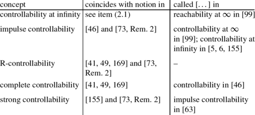
  Some of these aforementioned articles introduce the controllability by means of certain rank criteria for the matrix triple [E,A,B]. The connection of the concepts introduced in Definition 2.1 to linear algebraic properties of E, A and B will be highlighted in Sect. 4.

  For general DAE systems we have

  

  Our behavioral controllability coincides with the framework which is introduced in [128, Definition 5.2.2] for so-called differential behaviors, which are general (possibly higher order) DAE systems with constant coefficients. Note that the concept of behavioral controllability does not require a distinction between input and state. The concepts of reachability and controllability in [11–14] coincide with our behavioral and complete controllability, resp. (see Sect. 4). Full controllability of [171] is our complete controllability together with the additional assumption that solutions have to be unique.

• (ii) Stabilizability in the behavioral sense is introduced in [128, Definition 5.2.2]. For regular systems, stabilizability is usually defined either via linear algebraic properties of E, A and B, or by the existence of a stabilizing state feedback, see [33, 34, 57] and [49, Definition 3-1.2]. Our concepts of behavioral stabilizability and stabilizability coincide with the notions of internal stability and complete stabilizability, resp., defined in [114] for the system with , , z(t)=[x ^⊤(t),u ^⊤(t)]^⊤.

• (iii) Other concepts, not related to the ones considered in this article, are e.g. the instantaneous controllability (reachability) of order k in [120] or the impulsive mode controllability in [71]. Furthermore, the concept of strong controllability introduced in [147, Exercise 8.5] for ODE systems differs from the concepts considered in this article.

• (iv) The notion of consistent initial conditions is the most important one for DAE systems and therefore the consideration of the space (for B=0 when no control systems were considered) is as old as the theory of DAEs itself, see e.g. [60]. is sometimes called viability kernel [30], see also [8, 9]. The reachability and controllability space are some of the most important notions for (DAE) control systems and have been considered in [99] for regular systems. They are the fundamental subspaces considered in the geometric theory, see Sect. 6. Further usage of these concepts can be found in the following: in [122] generalized reachability and controllability subspaces of regular systems are considered; Eliopoulou and Karcanias [56] consider reachability and almost reachability subspaces of general DAE systems; Frankowska [58] considers the reachability subspace in terms of differential inclusions.

  A nice formula for the reachability space of a regular system has been derived by Yip et al. [169] (and later been adopted by Cobb [46], however, called controllable subspace): Consider a regular system [E,A,B]∈Σ _n,n,m in Weierstraß form [60], that is,

  $$E= \left[\begin{array}{c@{\quad}c} I_{n_1}&0\\ 0&N \end{array}\right] ,\qquad A= \left[\begin{array}{c@{\quad}c} J&0 \\ 0&I_{n_2} \end{array}\right] , \qquad B= \left[\begin{array}{c} B_1\\ B_2 \end{array}\right] , $$

  where N is nilpotent. Then [169, Thm. 2]

  

  where $\langle K | L \rangle:= \operatorname{im}_{\mathbb{R}}[L, KL, \ldots, K^{n-1} L]$ for some matrices $K\in{\mathbb{R}}^{n\times n}$, ${L\in{\mathbb {R}}^{n\times m}}$. Furthermore, we have [169, Thm. 3]

  

  This result has been improved later in [41] so that the Weierstraß form is no longer needed. Denoting by E ^D the Drazin inverse of a given matrix ${E\in{\mathbb{R}}^{n\times n}}$ (see [39]), it is shown [41, Thm. 3.1] that, for A=I,

  

  where the consideration of A=I is justified by a certain (time-varying) transformation of the system [124]. We further have [41, Thm. 3.2]

  

  Yet another approach was followed by Cobb [42] who obtains that

  

  for some $\alpha\in{\mathbb{R}}$ with det(αE−A)≠0. A simple proof of this result can also be found in [170].

• (v) The notion comes from the possible impulsive behavior of solutions of (2.1), i.e., x may have jumps, when distributional solutions are permitted, see e.g. [46] as a very early contribution in this regard. Since these jumps have no effect on the solutions if they occur at the initial time and within the kernel of E this leads to the definition of . See also the definition of impulse controllability.

• (vi) Impulse controllability and controllability at infinity are usually defined by considering distributional solutions of (2.1), see e.g. [46, 61, 75], sometimes called impulsive modes, see e.g. [21, 71, 155]. For regular systems, impulse controllability has been introduced by Verghese et al. [155] (called controllability at infinity in this work) as controllability of the impulsive modes of the system, and later made more precise by Cobb [46], see also Armentano [5, 6] (who also calls it controllability at infinity) for a more geometric point of view. In [155] the authors do also develop the notion of strong controllability as impulse controllability with, additionally, controllability in the regular sense. Cobb [43] showed that under the condition of impulse controllability, the infinite eigenvalues of regular sE−A can be assigned via a state feedback u=Fx to arbitrary finite positions. Armentano [5] later showed how to calculate F. This topic has been further pursued in [94] in the form of invariant polynomial assignment.

  The name “controllability at infinity” comes from the claim that the system has no infinite uncontrollable modes: Speaking in terms of rank criteria (see also Sect. 4) the system [E,A,B]∈Σ _k,n,m is said to have an uncontrollable mode at $\frac {\alpha }{\beta}$ if, and only if, $\operatorname{rk}[\alpha E+ \beta A,B] < \operatorname{rk}[E,A,B]$ for some $\alpha, \beta\in{\mathbb{C}}$. If β=0, then the uncontrollable mode is infinite. Controllability at infinity has been introduced by Rosenbrock [137]—although he does not use this phrase—as controllability of the infinite frequency zeros. Later Cobb [46] compared the concepts of impulse controllability and controllability at infinity, see [46, Thm. 5]; the notions we use in the present article go back to the distinction in this work.

  The concepts have later been generalized by Geerts [61] (see [61, Thm. 4.5 & Rem. 4.9], however, he does not use the name “controllability at infinity”). Controllability at infinity of (2.1) is equivalent to the strictness of the corresponding differential inclusion [58, Prop. 2.6]. The concept of impulsive mode controllability in [71] is even weaker than impulse controllability.

• (vii) Controllability concepts with a distributional solution setup have been considered in [61, 120, 130] for instance, see also [46]. A typical argumentation in these works is that inconsistent initial values cause distributional solutions in a way that the state trajectory is composed of a continuous function and a linear combination of Dirac’s delta impulse and some of its derivatives. However, some frequency domain considerations in [116] refute this approach (see [145] for an overview on inconsistent initialization). This justifies that we do only consider weakly differentiable solutions as defined in the behavior .

  Distributional solutions for time-invariant DAEs have already been considered by Cobb [44] and Geerts [61, 62] and for time-varying DAEs by Rabier and Rheinboldt [132]. For a mathematically rigorous approach to distributional solution theory of linear DAEs we refer to [143, 144] by Trenn. The latter works introduce the notions of impulse controllability and jump controllability which coincide with our impulse controllability and behavioral controllability, resp.

• (vii) R-controllability has been first defined in [169] for regular DAEs. Roughly speaking, R-controllability is the property that any consistent initial state x ₀ can be steered to any reachable state x _f , where here x _f is reachable if, and only if, there exist t>0 and such that x(t)=x _f ; by (2.3) the latter is equivalent to , as stated in Definition 2.1.

• (viii) The concept of behavioral controllability has been introduced by Willems [160], see also [128]. This concept is very suitable for generalizations in various directions, see e.g. [35, 40, 72, 97, 133, 163, 167]. Having found the behavior of the considered control system one can take over the definition of behavioral controllability without the need for any further changes. From this point of view this appears to be the most natural of the controllability concepts. However, this concept also seems to be the least regarded in the DAE literature.

• (ix) The controllability theory of DAE systems can also be treated with the theory of differential inclusions [8, 9] as showed by Frankowska [58].

• (x) Karcanias and Hayton [85] pursued a special ansatz to simplify the system (2.1): provided that B has full column rank, we take a left annihilator N and a pseudoinverse B ^† of B (i.e., NB=0 and B ^† B=I) such that is invertible and then pre-multiply (2.1) by W, thus obtaining the equivalent system

  

  The reachability (controllability) properties of (2.1) may now be studied in terms of the pencil sNE−NA, which is called the restriction pencil [78], first introduced as zero pencil for the investigation of system zeros of ODEs in [91, 92], see also [88]. For a comprehensive study of the properties of the pencil sNE−NA see e.g. [84–87].

• (xi) Banaszuk and Przyłuski [11] have considered perturbations of DAE control systems and obtained conditions under which the sets of all completely controllable systems (systems controllable in the behavioral sense) within the set of all systems Σ _k,n,m contain an open and dense subset, or its complement contains an open and dense subset.

The following dependencies hold true between the concepts from Definition 2.1. Some further relations will be derived in Sect. 4.

Proposition 2.4

For any [E,A,B]∈Σ _k,n,m the following implications hold true:

If “⇒” holds, then “⇐” does, in general, not hold.

Proof

Since it is easy to construct counterexamples for any direction where in the diagram only “⇒” holds, we skip their presentation. The following implications are immediate consequences of Definition 2.1:

• completely controllable ⇒ controllable at infinity ⇒ impulse controllable,

• completely controllable ⇒ strongly controllable ⇒ impulse controllable,

• completely controllable ⇒ completely reachable ⇒ strongly reachable,

• strongly controllable ⇒ strongly reachable,

• completely stabilizable ⇒ controllable at infinity,

• strongly stabilizable ⇒ impulse controllable,

• completely stabilizable ⇒ strongly stabilizable.

It remains to prove the following assertions:

• (a) completely reachable ⇒ completely controllable,

• (b) strongly reachable ⇒ strongly controllable,

• (c) completely reachable ⇒ completely stabilizable,

• (d) strongly reachable ⇒ strongly stabilizable.

(a) Let $x_{0},x_{f}\in{\mathbb{R}}^{n}$. Then, by complete reachability of [E,A,B], there exist t>0 and some with x ₁(0)=0 and x ₁(t)=x ₀. Further, there exists with x ₂(0)=0 and x ₂(t)=x _f −x ₁(2t). By linearity and shift-invariance, we have

On the other hand, this trajectory fulfills x(0)=x ₁(t)+x ₂(0)=x ₀ and x(t)=x ₁(2t)+x ₂(t)=x _f .

(b) The proof of this statement is analogous to (a).

(c) By (a) it follows that the system is completely controllable. Complete controllability implies that there exists some t>0, such that for all $x_{0}\in{\mathbb{R}}^{n}$ there exists with x ₁(0)=x ₀ and x ₁(t)=0. Then, since (x,u) with

$$\bigl(x(\tau),u(\tau)\bigr)= \begin{cases} (x_1(\tau),u_1(\tau)),& \text{if }\tau\leq t,\\ (0,0),& \text{if }\tau\geq t \end{cases} $$

satisfies (cf. the proof of Lemma 2.1(a)), the system [E,A,B] is completely stabilizable.

(d) The proof of this statement is analogous to (c). □

3 Solutions, Relations and Normal Forms

In this section we give the definitions for system and feedback equivalence of DAE control systems (see [63, 137, 155]), revisit the solution theory of DAEs (see [96, 159] and also [22]), and state a normal form under system and feedback equivalence (see [105]). For the definition of a canonical and a normal form see Remark 3.2.

3.1 System and Feedback Equivalence

We define the essential concepts of system and feedback equivalence. System equivalence was first studied by Rosenbrock [137] (called restricted system equivalence in his work, see also [155]) and later became a crucial concept in the control theory of DAEs [24, 25, 63, 64, 69]. Feedback equivalence for DAEs seems to have been first considered in [63] to derive a feedback canonical form for regular systems, little later also in [105] (for general DAEs) where additionally also derivative feedback was investigated and respective canonical forms derived, see also Sect. 3.3.

Definition 3.1

(System and feedback equivalence)

Two systems [E _i ,A _i ,B _i ]∈Σ _k,n,m , i=1,2, are called

• system equivalent if, and only if,

  $$\exists W\in\mathbf{Gl}_k({\mathbb{R}}), T\in\mathbf {Gl}_n({\mathbb{R}}): \left[\begin{array}{c@{\quad}c} sE_1-A_1 & B_1 \end{array}\right] = W \left[\begin{array}{c@{\quad}c} sE_2-A_2 & B_2 \end{array}\right] \left[\begin{array}{c@{\quad}c} T & 0 \\ 0 & I_m \end{array}\right] ; $$

  we write

  $$[ E_1 , A_1 , B_1 ] \stackrel{W,T}{\sim_{se}} [ E_2 , A_2 , B_2 ] ; $$

• feedback equivalent if, and only if,

  $$ \begin{aligned} &\exists W\in\mathbf{Gl}_k({ \mathbb{R}}), T\in\mathbf {Gl}_n({\mathbb{R}}), V\in \mathbf{Gl}_m({\mathbb{R}}), F\in {\mathbb{R}}^{m,n}: \\ & \left[\begin{array}{c@{\quad}c} sE_1-A_1 & B_1 \end{array}\right] = W \left[\begin{array}{c@{\quad}c} sE_2-A_2 & B_2 \end{array}\right] \left[\begin{array}{c@{\quad}c} T & 0 \\ -F & V \end{array}\right] ; \end{aligned} $$

  (3.1)

  we write

  $$[ E_1 , A_1 , B_1 ] \stackrel{W,T,V,F}{\sim_{fe}} [ E_2 , A_2 , B_2 ] . $$

It is easy to observe that both system and feedback equivalence are equivalence relations on Σ _k,n,m . To see the latter, note that if $[ E_{1} , A_{1} , B_{1} ] \stackrel{W,T,V,F}{\sim_{fe}} [ E_{2} , A_{2} , B_{2} ]$, then

$$[ E_2 , A_2 , B_2 ] \stackrel{W^{-1}, T^{-1}, V^{-1}, -V^{-1}FT^{-1}}{\sim_{fe}} [ E_1 , A_1 , B_1 ]. $$

The behaviors of system and feedback equivalent systems are connected via

$$ \begin{aligned} &\text{If}\quad[ E_1 , A_1 , B_1 ] \stackrel{W,T}{\sim_{se}} [ E_2 , A_2 , B_2 ] ,\quad\text{then} \\ &(x,u)\in\mathfrak{B}_{[E_1,A_1,B_1]}\Leftrightarrow (Tx,u)\in \mathfrak{B}_{[E_2,A_2,B_2]} \\ &\text{If}\quad[ E_1 , A_1 , B_1 ] \stackrel{W,T,V,F}{\sim_{fe}} [ E_2 , A_2 , B_2 ] ,\quad\text{then} \\ &(x,u)\in\mathfrak{B}_{[E_1,A_1,B_1]}\Leftrightarrow (Tx,Fx+Vu)\in \mathfrak{B}_{[E_2,A_2,B_2]}. \end{aligned} $$

(3.2)

In particular, if $[ E_{1} , A_{1} , B_{1} ] \stackrel{W,T}{\sim_{se}} [ E_{2} , A_{2} , B_{2} ]$, then

Further, if $[ E_{1} , A_{1} , B_{1} ] \stackrel{W,T,V,F}{\sim_{fe}} [ E_{2} , A_{2} , B_{2} ]$, then

and properties of controllability at infinity, impulse controllability, R-controllability, behavioral controllability, behavioral stabilizability, complete controllability, complete stabilizability, strong controllability and strong stabilizability are invariant under system and feedback equivalence.

Remark 3.1

(Equivalence and minimality in the behavioral sense)

• (i) Another equivalence concept has been introduced by Willems in [161] (see also [128, Def. 2.5.2]): Two systems $[E_{i},A_{i},B_{i}]\in\varSigma_{k_{i},n,m}$, i=1,2, are called equivalent in the behavioral sense, if their behaviors coincide, i.e.,

  $$\mathfrak{B}_{[E_1,A_1,B_1]}=\mathfrak{B}_{[E_2,A_2,B_2]}. $$

  Note that, in particular, two systems being equivalent in the behavioral sense do not necessarily have the same number of equations. For instance, the following two systems are equivalent in the behavioral sense:

  $$\bigl[[0],[1],[0]\bigr],\qquad \left[ \left[\begin{array}{c}0\\1 \end{array}\right] , \left[\begin{array}{c}1\\0 \end{array}\right] , \left[\begin{array}{c}0\\0 \end{array}\right] \right]. $$

• (ii) It is shown in [128, Thm. 2.5.4] that for a unimodular matrix $U(s)\in{\mathbb{R}}[s]^{k,k}$ (that is, U(s) has a polynomial inverse), and [E,A,B]∈Σ _k,n,m , it holds $(x,u)\in\mathfrak{B}_{[E,A,B]}$ if, and only if,

  $$U\biggl(\frac{\mathrm{d}}{\mathrm{d}t}\biggr)E\dot{x}(t)=U\biggl(\frac{\mathrm{d}}{\mathrm{d}t} \biggr)Ax(t)+U\biggl(\frac{\mathrm{d}}{\mathrm{d}t}\biggr)Bu(t), $$

  where the differential operator $U(\frac{\mathrm{d}}{\mathrm{d}t})$ has to be understood in the distributional sense. The unimodular matrix U(s) can particularly been chosen in a way that

  $$U(s)\cdot \left[\begin{array}{c@{\quad}c}sE-A,&-B \end{array}\right] = \left[\begin{array}{c@{\quad}c}R_x(s)&R_u(s)\\0&0 \end{array}\right] , $$

  where $[R_{x}(s)\ R_{u}(s)] \in{\mathbb{R}}[s]^{l,n+m}$ has full row rank as a matrix in the field ${\mathbb{R}}(s)$ [128, Thm. 3.6.2]. It is shown that $R_{x}(\frac{\mathrm{d}}{\mathrm{d}t})x+R_{u}(\frac{\mathrm{d}}{\mathrm{d}t})u=0$ is minimal in the behavioral sense, i.e., it describes the behavior by a minimal number of l differential equations among all behavioral descriptions of $\mathfrak{B}_{[E,A,B]}$. By using a special normal form, we will later remark that for any [E,A,B]∈Σ _k,n,m , there exists a unimodular transformation from the left such that the resulting differential-algebraic system is minimal in the behavioral sense.

• (iii) Conversely, if two systems $[E_{i},A_{i},B_{i}]\in\varSigma_{k_{i},n,m}$, i=1,2 are equivalent in the behavioral sense, and, moreover, k ₁=k ₂, then there exists some unimodular $U(s)\in{\mathbb{R}}[s]^{k_{1},k_{1}}$, such that

  $$U(s)\cdot \left[\begin{array}{c@{\quad}c}sE_1-A_1,&-B_1 \end{array}\right] = \left[\begin{array}{c@{\quad}c}sE_2-A_2,&-B_2 \end{array}\right] . $$

  If [E _i ,A _i ,B _i ] i=1,2, contain different numbers of equations (such as, e.g., k ₁>k ₂), then one can first add k ₁−k ₂ equations of type “0=0” to the second system and, thereafter, perform a unimodular transformation leading from one system to another.

• (iv) Provided that a unimodular transformation of $E\dot {x}(t)=Ax(t)+Bu(t)$ again leads to a differential-algebraic system (that is, neither a derivative of the input nor a higher derivative of the state occurs), the properties of controllability at infinity, R-controllability, behavioral controllability, behavioral stabilizability, complete controllability, complete stabilizability are invariant under this transformation. However, since the differential variables may be changed under a transformation of this kind, the properties of impulse controllability, strong controllability and strong stabilizability are not invariant. We will see in Remark 3.11 that any [E,A,B]∈Σ _k,n,m is, in the behavioral sense, equivalent to a system that is controllable at infinity.

In order to study normal forms under system and feedback equivalence we introduce the following notation: For $k\in{\mathbb{N}}$ we introduce the matrices $N_{k}\in{\mathbb{R}}^{k,k}$, $K_{k},L_{k}\in{\mathbb {R}}^{k-1,k}$ with

Further, let $e_{i}^{[k]}\in{\mathbb{R}}^{k}$ be the ith canonical unit vector, and, for some multi-index ${\bf\alpha}=(\alpha_{1},\ldots,\alpha_{l})\in {\mathbb{N}}^{l}$, we define

$$\begin{aligned} N_\alpha&=\operatorname{diag}(N_{\alpha_1}, \ldots,N_{\alpha_l})\in {\mathbb{R}}^{|\alpha |,|\alpha |}, \\ K_\alpha&=\operatorname{diag}(K_{\alpha_1},\ldots,K_{\alpha_l}) \in {\mathbb{R}}^{|\alpha |-l,|\alpha|}, \\ L_\alpha&=\operatorname{diag}(L_{\alpha_1},\ldots,L_{\alpha_l}) \in {\mathbb{R}}^{|\alpha |-l,|\alpha|}, \\ E_{\alpha}&=\operatorname{diag}\bigl(e_{\alpha_1}^{[\alpha_1]}, \ldots ,e_{\alpha _l}^{[\alpha _l]}\bigr)\in{\mathbb{R}}^{|\alpha|,l}. \end{aligned} $$

Kronecker proved [93] that any matrix pencil $sE-A\in {\mathbb{R}} [s]^{k,n}$ can be put into a certain canonical form, called Kronecker canonical form nowadays, of which a more comprehensive proof has been provided by Gantmacher [60]. In the following we may use the quasi-Kronecker form derived in [22, 23], since in general the Kronecker canonical form is complex-valued even though the given pencil sE−A is real-valued, what we need to avoid. The obtained form then is not canonical anymore, but it is a normal form (see Remark 3.2).

Proposition 3.1

(Quasi-Kronecker form [22, 23, 60])

For any matrix pencil ${sE-A\in{\mathbb{R}}[s]^{k,n}}$, there exist $W\in\mathbf{Gl}_{k}({\mathbb{R}})$, $T\in\mathbf{Gl}_{n}({\mathbb {R}})$ such that

$$ W(sE-A)T = \left[\begin{array}{c@{\quad}c@{\quad}c@{\quad}c} sI_{n_s}-A_s & 0 & 0 & 0 \\ 0 & sN_{\alpha}-I_{|\alpha|} & 0 & 0\\ 0 & 0 & sK_{\beta}-L_{\beta} & 0 \\ 0 & 0 & 0 & sK_{\gamma}^\top-L_{\gamma}^\top \end{array}\right] $$

(3.3)

for some $A_{s}\in{\mathbb{R}}^{n_{s},n_{s}}$ and multi-indices $\alpha\in{\mathbb {N}}^{n_{\alpha}}$, $\beta \in{\mathbb{N}}^{n_{\gamma}}$, $\gamma\in{\mathbb{N}}^{n_{\gamma}}$. The multi-indices α,β,γ are uniquely determined by sE−A. Further, the matrix A _s is unique up to similarity.

The (components of the) multi-indices α,β,γ are often called minimal indices and elementary divisors and play an important role in the analysis of matrix pencils, see e.g. [60, 104, 105, 113], where the components of α are the orders of the infinite elementary divisors, the components of β are the column minimal indices and the components of γ are the row minimal indices. In fact, the number of column (row) minimal indices equal to one corresponds to the dimension of $\ker_{\mathbb{R}}E \cap\ker_{\mathbb{R}}A$ ($\ker_{\mathbb{R}} E^{\top}\cap\ker_{\mathbb{R}}A^{\top}$), or, equivalently, the number of zero columns (rows) in a quasi-Kronecker form of sE−A. Further, note that $sI_{n_{s}}-A_{s}$ may be further transformed into Jordan canonical form to obtain the finite elementary divisors.

Since the multi-indices $\alpha\in{\mathbb{N}}^{n_{\alpha}}$, $\beta \in{\mathbb{N}}^{n_{\gamma}}$, $\gamma\in{\mathbb{N}}^{n_{\gamma}}$ are well-defined by means of the pencil sE−A and, furthermore, the matrix A _s is unique up to similarity, this justifies the introduction of the following quantities.

Definition 3.2

(Index of sE−A)

Let the matrix pencil $sE-A\in{\mathbb{R}}[s]^{k,n}$ be given with quasi-Kronecker form (3.3). Then the index $\nu\in {\mathbb{N}}_{0}$ of sE−A is defined as

$$\nu=\max\{\alpha_1,\ldots,\alpha_{\ell(\alpha)}, \gamma_1,\ldots ,\gamma_{\ell(\gamma)}\}. $$

The index is larger or equal to the index of nilpotency ζ of N _α , i.e., ζ≤ν, $N_{\alpha}^{\zeta}=0$ and $N_{\alpha}^{\zeta -1}\neq0$. By means of the quasi-Kronecker form (3.3) it can be seen that the index of sE−A does not exceed one if, and only if,

$$ \operatorname{im}_{\mathbb{R}}A\subseteq \operatorname{im}_{\mathbb{R}}E + A\cdot\ker_{\mathbb{R}} E. $$

(3.4)

This is moreover equivalent to the fact that for some (and hence any) real matrix Z with $\operatorname{im}_{\mathbb{R}}Z=\ker_{\mathbb {R}}E$, we have

$$ \operatorname{im}_{\mathbb{R}}[E, AZ]=\operatorname {im}_{\mathbb{R}}[E,A]. $$

(3.5)

Since each block in sK _β −L _β ($sK_{\gamma}^{\top}-L_{\gamma }^{\top}$) causes a single drop of the column (row) rank of sE−A, we have

$$ \ell(\beta)=n-\operatorname{rk}_{{\mathbb{R}}(s)}(sE-A), \qquad\ell (\gamma)=k-\operatorname{rk}_{{\mathbb{R}}(s)}(sE-A). $$

(3.6)

Further, $\lambda\in{\mathbb{C}}$ is a generalized eigenvalue of sE−A if, and only if,

$$\operatorname{rk}_{{\mathbb{C}}}(\lambda E-A)<\operatorname {rk}_{{\mathbb{R}}(s)}(sE-A). $$

3.2 A Normal Form Under System Equivalence

Using Proposition 3.1 it is easy to determine a normal form under system equivalence. For regular systems this normal form was first discovered by Rosenbrock [137].

Corollary 3.2

(Decoupled DAE)

Let [E,A,B]∈Σ _k,n,m . Then there exist $W\in\mathbf{Gl}_{k}({\mathbb{R}})$, $T\in\mathbf {Gl}_{n}({\mathbb{R}})$ such that

$$ [E,A,B] \stackrel{W,T}{ \sim_{se}} \left[ \left[\begin{array}{c@{\quad}c@{\quad}c@{\quad}c} I_{n_s} & 0 & 0 & 0\\ 0 & N_\alpha& 0 & 0\\ 0 & 0 & K_{\beta} & 0\\ 0 & 0 & 0 & K^\top_{\gamma} \end{array}\right] , \left[\begin{array}{c@{\quad}c@{\quad}c@{\quad}c} A_s & 0 & 0 & 0 \\ 0 & I_{|\alpha|} & 0 & 0\\ 0 & 0 & L_{\beta} & 0\\ 0 & 0 & 0 & L^\top_{\gamma} \end{array}\right] , \left[\begin{array}{c} B_s \\ B_f \\ B_u \\ B_o \end{array}\right] \right], $$

(3.7)

for some $B_{s}\in{\mathbb{R}}^{n_{s},m}$, $B_{f}\in{\mathbb{R}}^{|\alpha|,m}$, $B_{o}\in{\mathbb{R}}^{|\beta |-\ell (\beta),m}$, $B_{u}\in{\mathbb{R}}^{|\gamma|,m}$, $A_{s}\in{\mathbb{R}}^{n_{s},n_{s}}$ and multi-indices $\alpha\in{\mathbb {N}}^{n_{\alpha}}$, $\beta \in{\mathbb{N}}^{n_{\beta}}$, $\gamma\in{\mathbb{N}}^{n_{\gamma}}$. This is interpreted, in terms of the DAE (2.1), as follows: $(x,u)\in\mathfrak{B}_{[E,A,B]}$ if, and only if,

$$\bigl( x_s(\cdot)^\top, x_f( \cdot)^\top, x_u(\cdot)^\top, x_o(\cdot )^\top \bigr)^\top:= T x(\cdot) $$

with

$$x_f(\cdot)= \begin{pmatrix} x_{f[1]}(\cdot) \\ \vdots\\ x_{f[\ell(\alpha )]}(\cdot) \end{pmatrix} ,\qquad x_u(\cdot)= \begin{pmatrix} x_{u[1]}(\cdot) \\ \vdots\\ x_{u[\ell(\beta )]}(\cdot) \end{pmatrix} ,\qquad x_o(\cdot)= \begin{pmatrix} x_{o[1]}(\cdot) \\ \vdots\\ x_{o[\ell(\gamma )]}(\cdot) \end{pmatrix} $$

solves the decoupled DAEs

(3.8a)

(3.8b)

(3.8c)

(3.8d)

with suitably labeled partitions of B _f , B _u and B _o .

Remark 3.2

(Canonical and normal form)

Recall the definition of a canonical form: given a group G, a set , and a group action which defines an equivalence relation $s \stackrel{\alpha}{\sim} s'$ if, and only if, ∃U∈G:α(U,s)=s′. Then a map is called a canonical form for α [28] if, and only if,

Therefore, the set is divided into disjoint orbits (i.e., equivalence classes) and the mapping γ picks a unique representative in each equivalence class. In the setup of system equivalence, the group is $G= \mathbf {Gl}_{n}({\mathbb{R}})\times \mathbf{Gl}_{n}({\mathbb{R}})$, the considered set is and the group action α((W,T),[E,A,B])=[WET,WAT,WB] corresponds to $\stackrel{W^{-1},T^{-1}}{\sim}$. However, Corollary 3.2 does not provide a mapping γ. That means that the form (3.7) is not a unique representative within the equivalence class and hence it is not a canonical form. Nevertheless, we may call it a normal form, since every entry is (at least) unique up to similarity.

Remark 3.3

(Canonical forms for regular systems)

For regular systems which are completely controllable two actual canonical forms of [E,A,B]∈Σ _n,n,m under system equivalence have been obtained: the Jordan control canonical form in [64] and, later, the more simple canonical form in [69] based on the Hermite canonical form for controllable ODEs [I,A,B].

Remark 3.4

(DAEs corresponding to the blocks in the quasi-Kronecker form)

Corollary 3.2 leads to the separate consideration of the differential-algebraic equations (3.8a)–(3.8c):

• (i) (3.8a) is an ordinary differential equation whose solution satisfies

  $$x_s(t)=e^{A_st}x_s(0)+\int _0^te^{A_s(t-\tau)}B_su(\tau)\,\mathrm{d} \tau, \quad t\in {\mathbb{R}}. $$

  In particular, solvability is guaranteed by . The initial value $x_{s}(0)\in {\mathbb{R}}^{n}$ can be chosen arbitrarily; the prescription of and $x_{s}(0)\in{\mathbb{R}}^{n}$ guarantees uniqueness of the solution.

• (ii) The solutions of (3.8b) can be calculated by successive differentiation and pre-multiplication with $N_{\alpha_{i}}$, hence we have

  

  where u ^(j) denotes the jth distributional derivative of u. As a consequence, the solution requires a certain smoothness of the input, expressed by

  

  In particular, condition guarantees solvability of the DAE (3.8b). Note that the initial value x _f[i](0) cannot be chosen at all: It is fixed by u via the relation

  $${x}_{f[i]}(0)= - \Biggl(\sum_{j=0}^{\alpha_i-1} N_{\alpha_i}^{j} {B}_{f[i]}u^{(j)} \Biggr) (0). $$

  On the other hand, for any (sufficiently smooth) input there exists a unique solution for appropriately chosen initial value.

• (iii) Writing

  $${x}_{u[i]-}= \left[\begin{array}{c}{x}_{u[i],1}\\\vdots\\{x}_{u[i],\beta_i-1} \end{array}\right] , $$

  (3.8c) is equivalent to

  $$\dot{x}_{u[i]-}=N_{\beta_i-1}^\top{x}_{u[i]-}+e_{\beta_i-1}^{[\beta _i-1]}{x}_{u[i],\beta_i}+B_{u[i]}u(t). $$

  Hence, a solution exists for all inputs and all as well as ${x}_{u[i],1}(0),\ldots,{x}_{u[i],\beta_{i}-1}(0)$. This system is therefore underdetermined in the sense that one component as well as all initial values can be freely chosen. Hence any existing solution for fixed input u and fixed initial value x _u[i](0) is far from being unique.

• (iv) Denoting

  $${x}_{o[i]+}= \left[\begin{array}{c} 0_{1,1}\\ {x}_{o[i]} \end{array}\right] , $$

  (3.8d) can be rewritten as

  $$N_{\gamma_i }^\top\dot{x}_{o[i]+}={x}_{o[i]+}+{B}_{o[i]}u(t). $$

  Hence we obtain ${x}_{o[i]+}(t)=-\sum_{j=0}^{\gamma_{i}-1} (N_{\gamma _{i}}^{\top})^{j} {B}_{o[i]}u^{(j)}(t)$, which gives

  $${x}_{o[i]}(t)=-[0_{(\gamma_i-1),1}, I_{\gamma_i-1}] \sum _{j=0}^{\gamma _i-1} \bigl(N_{\gamma_i}^\top \bigr)^{j} {B}_{o[i]}u^{(j)}(t) $$

  together with the consistency condition on the input:

  $$ \bigl(e_{1}^{[\gamma_i]} \bigr)^\top\sum_{j=0}^{\gamma_i-1} \bigl(N_{\gamma _i}^\top\bigr)^{j} {B}_{o[i]}u^{(j)}(t) = 0. $$

  (3.9)

  The smoothness condition

  

  is therefore not enough to guarantee existence of a solution; the additional constraint formed by (3.9) has to be satisfied, too. Furthermore, as in (ii), the initial value x _o[i](0) is fixed by the input u. Hence, a solution does only exist if the consistency conditions on the input and initial value are satisfied, but then the solution is unique.

Remark 3.5

(Solutions on (finite) time intervals)

The solution of a DAE [E,A,B]∈Σ _k,n,m on some time interval $I\subsetneq{\mathbb{R}}$ can be defined in a straightforward manner (compare (2.2)). By the considerations in Remark 3.4, we can infer that any solution (x,u) on some finite time interval $I\subsetneq{\mathbb{R}}$ can be extended to a solution on the whole real axis. Consequently, all concepts which have been defined in Sect. 2 could be also made based on solutions on intervals I including zero.

3.3 A Normal Form under Feedback Equivalence

A normal form under feedback transformation (3.1) was first studied for systems governed by ordinary differential equations by Brunovský [32]. In this section we present a generalization of the Brunovský form for general DAE systems [E,A,B]∈Σ _k,n,m from [105]. For more details of the feedback form and a more geometric point of view on feedback invariants and feedback canonical forms see [87, 105].

Remark 3.6

(Feedback for regular systems)

It is known [12, 63] that the class of regular DAE systems is not closed under the action of state feedback. Therefore, in [140] the class of regular systems is divided into the families

$$\varSigma_\theta:= \bigl\{ (E,A,B) \in\varSigma_{n,n,m}\mid \det( \cos \theta E - \sin \theta A) \neq0 \bigr\},\quad\theta\in[0,\pi), $$

and it is shown that any of these families is dense in the set of regular systems and the union of these families is exactly the set of regular systems. The authors of [140] then introduce the “constant-ratio proportional and derivative” feedback on Σ _θ , i.e.

$$u = F (\cos\theta x - \sin\theta \dot{x}) + v. $$

This feedback leads to a group action and enables them to obtain a generalization of Brunovský’s theorem [32] on each of the subsets of completely controllable systems in Σ _θ , see [140, Thm. 6].

Glüsing-Lüerßen [63] derived a canonical form under the unchanged feedback equivalence (3.1) on the set of strongly controllable (called impulse controllability in [63]) regular systems, see [63, Thm. 4.7]. In particular it was shown that this set is closed under the action of a feedback group.

Theorem 3.3

(Normal form under feedback equivalence [105])

Let [E,A,B]∈Σ _k,n,m . Then there exist $W\in\mathbf{Gl}_{k}({\mathbb{R}}), T\in\mathbf {Gl}_{n}({\mathbb{R}}), V\in\mathbf{Gl}_{m}({\mathbb{R}}), F\in {\mathbb{R}}^{m,n}$ such that

(3.10)

for some multi-indices α,β,γ,δ,κ and a matrix $A_{\overline{c}}\in{\mathbb{R}}^{n_{\overline{c}},n_{\overline{c}}}$. This is interpreted, in terms of the DAE (2.1), as follows: $(x,u)\in\mathfrak{B}_{[E,A,B]}$ if, and only if,

with

solves the decoupled DAEs

(3.11a)

(3.11b)

(3.11c)

(3.11d)

(3.11e)

(3.11f)

Note that by Remark 3.2 the form (3.10) is a normal form. However, if we apply an additional state space transformation to the block $[ I_{n_{\overline{c}}}, A_{\overline{c}}, 0]$ which puts $A_{\overline{c}}$ into Jordan canonical form, and then prescribe the order of the blocks of each type, e.g. from largest dimension to lowest (what would mean α ₁≥α ₂≥⋯≥α _ℓ(α) for α for instance), then (3.10) becomes a canonical form.

Remark 3.7

(DAEs corresponding to the blocks in the feedback form)

The form in Theorem 3.3 again leads to the separate consideration of the differential-algebraic equations (3.11a)–(3.11f):

• (i) (3.11a) is given by $[I_{\alpha_{i}},N_{\alpha_{i}}^{\top},e_{\alpha_{i}}^{[\alpha_{i}]}]$, and is completely controllable by the classical results for ODE systems (see e.g. [147, Sect. 3.2]). This system has furthermore the properties of being R-controllable, and both controllable and stabilizable in the behavioral sense.

• (ii) (3.11b) corresponds to an underdetermined system with zero dimensional input space. Since x _u[i] satisfies (3.11b) if, and only if, there exists some with

  $$\dot{x}_{u[i]}(t) = N_{\beta_i}^\top x_{u[i]}(t)+e_{\beta_i}^{[\beta_i]} v_i(t), $$

  this system has the same properties as (3.11a).

• (iii) Denoting

  $${z}_{ob[i]}= \left[\begin{array}{c}{x}_{ob[i]}\\ u_{ob[i]} \end{array}\right] , $$

  then (3.11c) can be rewritten as

  $$N_{\gamma_i }\dot{z}_{ob[i]}(t)={z}_{ob[i]}(t), $$

  which has, by (ii) in Remark 3.4, the unique solution z _ob[i]=0. Hence,

  $$\mathfrak{B}_{[L_{\gamma_i}^\top,K_{\gamma_i}^\top,e_{\gamma _i}^{[\gamma _i]}]}=\{0\}. $$

  The system $[L_{\gamma_{i}}^{\top},K_{\gamma_{i}}^{\top},e_{\gamma _{i}}^{[\gamma _{i}]}]$ is therefore completely controllable if, and only if, γ _i =1. In the case where γ _i >1, this system is not even impulse controllable. However, independent of γ _i , $[L_{\gamma_{i}}^{\top},K_{\gamma_{i}}^{\top},e_{\gamma_{i}}^{[\gamma_{i}]}]$ is R-controllable, and both controllable and stabilizable in the behavioral sense.

• (iv) Again, we have

  $$\mathfrak{B}_{[K_{\delta_i}^\top,L_{\delta_i}^\top,0_{\delta _i,0}]}=\{ 0\}, $$

  whence, in dependence on δ _i , we can infer the same properties as in (iii).

• (v) Due to

  $$\mathfrak{B}_{[N_{\kappa_i},I_{\kappa_i},0_{\kappa_i,0}]}=\{0\}, $$

  the system $[N_{\kappa_{i}},I_{\kappa_{i}},0_{\kappa_{i},0}]$ is never controllable at infinity, but always R-controllable and both controllable and stabilizable in the behavioral sense. $[N_{\kappa _{i}},I_{\kappa_{i}},0_{\kappa_{i},0}]$ is strongly controllable if, and only if, κ _i =1.

• (vi) The system $[I_{n_{\overline{c}}},A_{\overline{c}},0_{\overline {c},0}]$ satisfies

  $$\mathfrak{B}_{[I_{n_{\overline{c}}},A_{\overline{c}},0_{n_{\overline {c}},0}]}= \bigl\{ e^{A_{\overline{c}} \cdot}x^{0}\bigm{|} x^{0}\in{\mathbb{R}}^{n_{\overline{c}}} \bigr\}, $$

  whence it is controllable at infinity, but neither strongly controllable nor controllable in the behavioral sense nor R-controllable. The properties of being complete and strong stabilizability and stabilizability in the behavioral sense are attained if, and only if, $\sigma(A_{\overline{c}})\subseteq{\mathbb{C}}_{-}$.

By using the implications shown in Proposition 2.4, we can deduce the following for the systems arising in the feedback form:

Corollary 3.4

A system [E,A,B]∈Σ _k,n,m with feedback form (3.10) is

• (a) controllable at infinity if, and only if, γ=(1,…,1), δ=(1,…,1) and ℓ(κ)=0;

• (b) impulse controllable if, and only if, γ=(1,…,1), δ=(1,…,1) and κ=(1,…,1);

• (c) strongly controllable (and thus also strongly reachable) if, and only if, γ=(1,…,1), δ=(1,…,1), κ=(1,…,1) and $n_{\overline{c}}=0$;

• (d) completely controllable (and thus also completely reachable) if, and only if, γ=(1,…,1), δ=(1,…,1) and $\ell (\kappa)=n_{\overline{c}}=0$;

• (e) R-controllable if, and only if, $n_{\overline{c}}=0$;

• (f) controllable in the behavioral sense if, and only if, $n_{\overline{c}}=0$;

• (g) strongly stabilizable if, and only if, γ=(1,…,1), δ=(1,…,1), ℓ(κ)=0, and $\sigma(A_{\overline {c}})\subseteq{\mathbb{C}}_{-}$;

• (h) completely stabilizable if and only if, γ=(1,…,1), δ=(1,…,1), κ=(1,…,1), and $\sigma (A_{\overline {c}})\subseteq{\mathbb{C}}_{-}$;

• (i) stabilizable in the behavioral sense if, and only if, $\sigma (A_{\overline{c}})\subseteq{\mathbb{C}}_{-}$.

Remark 3.8

(Parametrization of the behavior of systems in feedback form)

With the findings in Remark 3.7, we may explicitly characterize the behavior of systems in feedback form. Define

$$V_{k}(s)=\bigl[1, s, \ldots, s^k\bigr]^\top \in{\mathbb{R}}[s]^{k,1} $$

and, for some multi-index $\mu=(\mu_{1},\ldots,\mu_{l})\in{\mathbb{N}}^{l}$,

$$\begin{aligned} V_\mu(s)&= \operatorname{diag} \bigl(V_{\mu_1}(s),\ldots,V_{\mu _l}(s)\bigr)\in{\mathbb{R}} [s]^{|\mu|,\ell (\mu)}, \\ W_\mu(s)&= \operatorname{diag}\bigl(s^{\mu_1}, \ldots,s^{\mu _l}\bigr)\in{\mathbb{R}} [s]^{\ell (\mu),\ell(\mu)}. \end{aligned} $$

Further let μ+k:=(μ ₁+k,…,μ _l +k) for $k\in{\mathbb {Z}}$, and

Then the behavior of a system in feedback form can, formally, be written as

where the sizes of the blocks are according to the block structure in the feedback form (3.10) and the horizontal line is the dividing line between x- and u-variables. If the system [E,A,B]∈Σ _k,n,m is not in feedback form, then a parametrization of the behavior can be found by using the above representation and relation (3.2) expressing the connection between behaviors of feedback equivalent systems.

For general differential behaviors, a parametrization of the above kind is called image representation [128, Sect. 6.6].

Remark 3.9

(Derivative feedback)

A canonical form under proportional and derivative feedback (PD feedback) was derived in [105] as well (note that PD feedback defines an equivalence relation on Σ _k,n,m ). The main tool for doing this is the restriction pencil (see Remark 2.1(xi)): Clearly, the system

is equivalent, via PD feedback, to the system

Then putting sNE−NA into Kronecker canonical form yields a PD canonical form for the DAE system with a 5×4-block structure.

We may, however, directly derive this PD canonical form from the normal form (3.10). To this end we may observe that the system $[I_{\alpha_{i}},N_{\alpha_{i}}^{\top},e_{\alpha_{i}}^{[\alpha_{i}]}]$ can be written as

$$K_{\alpha_i} \dot{x}_{c[i]}(t) = L_{\alpha_i} x_{c[i]}(t),\qquad\dot{x}_{c[i],\alpha_i}(t) = u_{c[i]}(t), $$

and hence is, via PD feedback, equivalent to the system

$$\left[ \left[\begin{array}{c} K_{\alpha_i}\\ 0 \end{array}\right] , \left[\begin{array}{c} L_{\alpha_i}\\ 0 \end{array}\right] , \left[\begin{array}{c} 0\\ 1 \end{array}\right] \right]. $$

On the other hand, the system $[L_{\gamma_{i}}^{\top},K_{\gamma_{i}}^{\top},e_{\gamma_{i}}^{[\gamma_{i}]}]$ can be written as

$$N_{\gamma_i-1} \dot{x}_{ob[i]}(t) = x_{ob[i]}(t),\qquad\dot{x}_{ob[i],\gamma_{i-1}}(t) = u_{ob[i]}(t), $$

and hence is, via PD feedback, equivalent to the system

$$\left[ \left[\begin{array}{c} N_{\gamma_i-1} \\ 0 \end{array}\right] , \left[\begin{array}{c} I_{\gamma_i-1}\\ 0 \end{array}\right] , \left[\begin{array}{c} 0\\ 1 \end{array}\right] \right]. $$

A canonical form for [E,A,B]∈Σ _k,n,m under PD feedback is therefore given by

$$[E,A,B] \sim_{PD} \left[ \left[\begin{array}{c@{\quad}c@{\quad}c@{\quad}c} K_{\beta} & 0 & 0 & 0\\* 0 & K_{\delta}^\top& 0 & 0 \\ 0 & 0 & N_\kappa& 0 \\ 0 & 0 & 0 & I_{n_{\overline{c}}}\\ 0&0&0&0 \end{array}\right] , \left[\begin{array}{c@{\quad}c@{\quad}c@{\quad}c}L_{\beta} & 0 & 0 & 0\\* 0 & L_{\delta}^\top& 0 & 0 \\ 0 & 0 & I_{|\kappa|} & 0 \\ 0 & 0 & 0 & A_{\overline{c}} \\ 0&0&0&0 \end{array}\right] , \left[\begin{array}{c@{\quad}c} 0&0 \\ 0&0 \\ 0&0\\ 0&0\\ I_{\zeta}& 0 \end{array}\right] \right], $$

where $A_{\overline{c}}$ is in Jordan canonical form, and the blocks of each type are ordered from largest dimension to lowest.

Note that the properties of complete controllability, controllability at infinity and controllability in the behavioral sense are invariant under PD feedback. However, since derivative feedback changes the set of differential variables, the properties of strong controllability as well as impulse controllability may be lost/gained after PD feedback.

Remark 3.10

(Connection to Kronecker form)

We may observe from (3.1) that feedback transformation may be alternatively considered as a transformation of the extended pencil

(3.12)

that is based on a multiplication from the left by , and from the right by

This equivalence is therefore a subclass of the class which is induced by the pre- and post-multiplication of by arbitrary invertible matrices. Loosely speaking, one can hence expect a normal form under feedback equivalence which specializes the quasi-Kronecker form of . Indeed, the latter form may be obtained from the feedback form of [E,A,B] by several simple row transformations which are not interpretable as feedback group actions anymore. More precisely, simple permutations of columns lead to the separate consideration of the extended pencils corresponding to the systems (3.11a)–(3.11f): The extended pencils corresponding to $[I_{\alpha _{i}},N_{\alpha_{i}}^{\top},e_{\alpha_{i}}^{[\alpha_{i}]}]$ and $[K_{\beta_{i}},L_{\beta_{i}},0_{\alpha_{i},0}]$ are $sK_{\alpha _{i}}-L_{\alpha_{i}}$ and $sK_{\beta_{i}}-L_{\beta_{i}}$, resp. The extended matrix pencil corresponding to the system $[L_{\gamma_{i}}^{\top},K_{\gamma_{i}}^{\top},e_{\gamma_{i}}^{[\gamma_{i}]}]$ is given by $sN_{\gamma_{i}}-I_{{\gamma_{i}}}$. The extended matrix pencils corresponding to the systems $[K_{\delta_{i}}^{\top},L_{\delta_{i}}^{\top},0_{\delta_{i},0}]$, $[N_{\kappa_{i}},I_{\kappa_{i}},0_{\kappa_{i},0}]$ and $[I_{n_{\overline {c}}},A_{\overline{c}},0_{\overline{c},0}]$ are obviously given by $sK_{\delta_{i}}^{\top}-L_{\delta_{i}}^{\top}$, $sN_{\kappa_{i}}-I_{\kappa_{i}}$ and $sI_{n_{\overline{c}}}-A_{\overline {c}}$, respectively. In particular, $\lambda\in{\mathbb{C}}$ is a generalized eigenvalue of , if, and only if, $\lambda \in \sigma(A_{\overline{c}})$.

Remark 3.11

(Minimality in the behavioral sense)

• (i) According to Remark 3.1, a differential-algebraic system [E,A,B]∈Σ _k,n,m is minimal in the behavioral sense, if, and only if, the extended pencil as in (3.12) has full row rank as a matrix with entries in the field ${\mathbb {R}}(s)$. On the other hand, a system [E,A,B]∈Σ _k,n,m with feedback form (3.10) satisfies

  

  Using that is invariant under feedback transformation (3.1), we can conclude that minimality of [E,A,B]∈Σ _k,n,m in the behavioral sense corresponds to the absence of blocks of type (3.11d) in its feedback form.

• (ii) The findings in Remark 3.4 imply that a system in feedback form is, in the behavioral sense, equivalent to

  

  This system can alternatively be achieved by multiplying the extended pencil (3.12) in feedback form (3.10) from the left with the polynomial matrix

  $$Z(s)=\operatorname{diag} \Biggl(I_{|\alpha|}, I_{|\beta|-\ell (\beta)}, - \sum_{k=0}^{\nu_\gamma-1}s^kN_\gamma^k, P_{\delta}(s), -\sum_{k=0}^{\nu_\kappa-1}s^kN_\kappa^k, I_{n_{\overline{c}}} \Biggr), $$

  where ν _γ =max{γ ₁,…,γ _ℓ(γ)}, ν _κ =max{κ ₁,…,κ _ℓ(κ)}, and

  $$P_{\delta}(s)= \operatorname{diag} \left( \left[\begin{array}{c@{\quad}c} 0_{\delta_i-1,1},&\displaystyle-\sum_{k=0}^{\delta _i-2}s^k (N_{\delta_i-1}^\top )^k \end{array}\right] \right)_{j=1,\ldots, \ell(\delta)}. $$

• (iii) Let a differential-algebraic system [E,A,B]∈Σ _k,n,m be given. Using the notation from (3.10) and the previous item, a behaviorally equivalent and minimal system [E _M ,A _M ,B _M ]∈Σ _{k−ℓ(δ),n,m} can be constructed by

  $$\left[\begin{array}{c@{\quad}c}sE_M-A_M,&-B_M \end{array}\right] =Z(s)W \left[\begin{array}{c@{\quad}c}sE-A,&-B \end{array}\right] . $$

  It can be seen that this representation is furthermore controllable at infinity. As well, it minimizes, among all differential-algebraic equations representing the same behavior, the index and the rank of the matrix in front of the state derivative (that is, loosely speaking, the number of differential variables). This procedure is very closely related to index reduction [96, Sect. 6.1].

4 Criteria of Hautus Type

In this section we derive equivalent criteria on the matrices $E,A\in {\mathbb{R}}^{k,n}$, $B\in{\mathbb{R}}^{k,m}$ for the controllability and stabilizability concepts of Definition 2.1. The criteria are generalizations of the Hautus test (also called Popov–Belevitch–Hautus test, since independently developed by Popov [129], Belevitch [17] and Hautus [68]) in terms of rank criteria on the involved matrices. Note that these conditions are not new—we refer to the relevant literature. However, we provide new proofs using only the feedback normal form (3.10).

First we show that certain rank criteria on the matrices involved in control systems are invariant under feedback equivalence. After that, we relate these rank criteria to the feedback form (3.10).

Lemma 4.1

Let [E ₁,A ₁,B ₁],[E ₂,A ₂,B ₂]∈Σ _k,n,m be given such that for $W\in\mathbf{Gl}_{k}({\mathbb{R}})$, $T\in\mathbf{Gl}_{n}({\mathbb {R}})$, $V\in\mathbf{Gl}_{m}({\mathbb{R}})$ and $F\in{\mathbb{R}}^{m,n}$, we have

$$[ E_1 , A_1 , B_1 ] \stackrel{W,T,V,F}{\sim_{fe}} [ E_2 , A_2 , B_2 ] . $$

Then

$$\begin{aligned} \operatorname{im}_{\mathbb{R}}E_1+ \operatorname{im}_{\mathbb{R}}A_1 +\operatorname{im}_{\mathbb{R}}B_1 =& W\cdot (\operatorname {im}_{\mathbb{R}}E_2 + \operatorname{im}_{\mathbb{R}} A_2 +\operatorname{im}_{\mathbb{R}}B_2 ), \\ \operatorname{im}_{\mathbb{R}}E_1 +A_1\cdot\ker_{\mathbb{R}}E_1 +\operatorname{im}_{\mathbb{R}}B_1 =& W\cdot (\operatorname{im}_{\mathbb{R}}E_2 +A_2 \cdot\ker_{\mathbb{R}}E_2 +\operatorname{im}_{\mathbb{R}}B_2 ), \\ \operatorname{im}_{\mathbb{R}}E_1 +\operatorname{im}_{\mathbb {R}}B_1 =& W\cdot (\operatorname{im}_{\mathbb{R}}E_2 + \operatorname{im}_{\mathbb{R}}B_2 ), \\ \operatorname{im}_{\mathbb{C}}(\lambda E_1-A_1)+ \operatorname {im}_{\mathbb{C}}B_1 =& W\cdot \bigl( \operatorname{im}_{\mathbb{C}} (\lambda E_2-A_2)+ \operatorname{im}_{\mathbb{C}}B_2 \bigr)\quad\text{\textit{for all} } \lambda\in{\mathbb{C}}, \\ \operatorname{im}_{{\mathbb{R}}(s)}(s E_1-A_1)+ \operatorname {im}_{{\mathbb{R}}(s)} B_1 =& W\cdot \bigl(\operatorname {im}_{{\mathbb{R}}(s)}(s E_2-A_2)+\operatorname{im}_{{\mathbb{R}}(s)} B_2 \bigr). \end{aligned} $$

Proof

Immediate from (3.1). □

Lemma 4.2

(Algebraic criteria via feedback form)

For a system [E,A,B]∈Σ _k,n,m with feedback form (3.10) the following statements hold true:

• (a)
  $$\begin{array}{ll}&\operatorname{im}_{\mathbb{R}}E +\operatorname {im}_{\mathbb{R}}A +\operatorname{im}_{\mathbb{R}}B =\operatorname {im}_{\mathbb{R}}E +\operatorname{im}_{\mathbb{R}} B\\ [2mm] \Longleftrightarrow& \gamma=(1,\ldots,1), \delta=(1,\ldots ,1), \ell(\kappa)=0. \end{array} $$
• (b)
  $$\begin{array}{ll}&\operatorname{im}_{\mathbb{R}}E +\operatorname {im}_{\mathbb{R}}A +\operatorname{im}_{\mathbb{R}}B =\operatorname {im}_{\mathbb{R}}E +A\cdot \ker_{\mathbb{R}} E +\operatorname{im}_{\mathbb{R}}B \\[2mm] \Longleftrightarrow& \gamma=(1,\ldots,1), \delta =(1,\ldots,1), \kappa=(1,\ldots,1). \end{array} $$
• (c)
  $$\begin{array}{ll}&\operatorname{im}_{\mathbb{C}}E +\operatorname {im}_{\mathbb{C}}A +\operatorname{im}_{\mathbb{R}}B =\operatorname {im}_{\mathbb{C}}(\lambda E-A)+\operatorname{im}_{\mathbb{C}}B \\[2mm] \Longleftrightarrow& \delta=(1,\ldots,1), \lambda \notin \sigma(A_{\overline{c}}). \end{array} $$

• (d) For $\lambda\in{\mathbb{C}}$ we have

  $$\begin{array}{ll} &\dim \bigl(\operatorname{im}_{{\mathbb {R}}(s)}(sE-A)+\operatorname{im}_{{\mathbb{R}}(s)} B \bigr)=\dim \bigl(\operatorname{im}_{\mathbb{C}}(\lambda E-A)+\operatorname{im}_{\mathbb{C}}B \bigr) \\[2mm] \Longleftrightarrow& \lambda\notin\sigma(A_{\overline{c}}). \end{array} $$

Proof

It is, by Lemma 4.1, no loss of generality to assume that [E,A,B] is already in feedback normal form. The results then follow by a simple verification of the above statements by means of the feedback form. □

Combining Lemmas 4.1 and 4.2 with Corollary 3.4, we may deduce the following criteria for the controllability and stabilizability concepts introduced in Definition 2.1.

Corollary 4.3

(Algebraic criteria for controllability/stabilizability)

Let a system [E,A,B]∈Σ _k,n,m be given. Then the following holds:

The above result leads to the following extension of the diagram in Proposition 2.4. Note that the equivalence of R-controllability and controllability in the behavioral sense was already shown in Corollary 3.4.

In the following we will consider further criteria for the concepts introduced in Definition 2.1.

Remark 4.1

(Controllability at infinity)

Corollary 4.3 immediately implies that controllability at infinity is equivalent to

$$\operatorname{im}_{\mathbb{R}}A \subseteq\operatorname{im}_{\mathbb {R}}E + \operatorname{im}_{\mathbb{R}}B . $$

In terms of a rank criterion, this is the same as

$$ \operatorname{rk}_{\mathbb{R}}[E,A,B]=\operatorname {rk}_{\mathbb{R}}[E,B]. $$

(4.1)

Criterion (4.1) has first been derived by Geerts [61, Thm. 4.5] for the case $\operatorname{rk}[E, A, B] = k$, although he does not use the name “controllability at infinity”.

In the case of regular $sE-A\in{\mathbb{R}}[s]^{n,n}$, condition (4.1) reduces to

$$\operatorname{rk}_{\mathbb{R}}[E,B]=n. $$

Remark 4.2

(Impulse controllability)

By Corollary 4.3, impulse controllability of [E,A,B]∈Σ _k,n,m is equivalent to

$$\operatorname{im}_{\mathbb{R}}A\subseteq\operatorname{im}_{\mathbb {R}}E + A\cdot\ker_{\mathbb{R}}E +\operatorname{im}_{\mathbb{R}}B . $$

Another equivalent characterization is that, for one (and hence any) matrix Z with $\operatorname{im}_{\mathbb{R}}(Z)=\ker_{\mathbb {R}}(E)$, we have

$$ \operatorname{rk}_{\mathbb{R}}[E,A,B]=\operatorname {rk}_{\mathbb{R}}[E,AZ,B]. $$

(4.2)

This has first been derived by Geerts [61, Rem. 4.9], again for the case $\operatorname{rk}[E, A, B] = k$. In [75, Thm. 3] and [71] the result has been obtained that impulse controllability is equivalent to

$$\operatorname{rk}_{\mathbb{R}} \left[\begin{array}{c@{\quad}c@{\quad}c} E&0&0\\ A&E&B \end{array}\right] = \operatorname{rk}_{\mathbb{R}}[E,A,B] + \operatorname{rk}_{\mathbb{R}}E, $$

which is in fact equivalent to (4.2). It has also been shown in [75, p. 1] that impulse controllability is equivalent to

This criterion can be alternatively shown by using the feedback form (3.10). Using condition (3.5) we may also infer that this is equivalent to the index of the extended pencil being at most one.

If the pencil sE−A is regular, then condition (4.2) reduces to

$$\operatorname{rk}_{\mathbb{R}}[E,AZ,B]=n. $$

This condition can be also inferred from [49, Th. 2-2.3].

Remark 4.3

(Controllability in the behavioral sense and R-controllability)

The concepts of controllability in the behavioral sense and R-controllability are equivalent by Corollary 3.4. The algebraic criterion for behavioral controllability in Corollary 4.3 is equivalent to the extended matrix pencil having no generalized eigenvalues, or, equivalently, in the feedback form (3.10) it holds $n_{\overline{c}}=0$.

The criterion for controllability in the behavioral sense is shown in [128, Thm. 5.2.10] for the larger class of linear differential behaviors. R-controllability for systems with regular sE−A was considered in [49, Thm. 2-2.2], where the condition

$$\operatorname{rk}_{\mathbb{C}}[\lambda E-A,B]=n\quad \forall\lambda \in{ \mathbb{C}} $$

was derived. This is, for regular sE−A, in fact equivalent to the criterion for behavioral stabilizability in Corollary 4.3.

Remark 4.4

(Complete controllability and strong controllability)

By Corollary 4.3, complete controllability of [E,A,B]∈Σ _k,n,m is equivalent to [E,A,B] being R-controllable and controllable at infinity, whereas strong controllability of [E,A,B]∈Σ _k,n,m is equivalent to [E,A,B] being R-controllable and impulse controllable.

Banaszuk et al. [12] already obtained the condition in Corollary 4.3 for complete controllability considering discrete systems. Complete controllability is called -controllability in [12]. Recently, Zubova [171] considered full controllability, which is just complete controllability with the additional assumption that solutions have to be unique, and obtained three equivalent criteria [171, Sect. 7], where the first one characterizes the uniqueness and the other two are equivalent to the condition for complete controllability in Corollary 4.3.

For regular systems, the conditions in Corollary 4.3 for complete and strong controllability are also derived in [49, Thm. 2-2.1 & Thm. 2-2.3].

Remark 4.5

(Stabilizability)

By Corollary 4.3, complete stabilizability of [E,A,B]∈Σ _k,n,m is equivalent to [E,A,B] being stabilizable in the behavioral sense and controllable at infinity, whereas strong stabilizability of [E,A,B]∈Σ _k,n,m is equivalent to [E,A,B] being stabilizable in the behavioral sense and impulse controllable.

The criterion for stabilizability in the behavioral sense is shown in [128, Thm. 5.2.30] for the class of linear differential behaviors.

Remark 4.6

(Kalman criterion for regular systems)

For regular systems [E,A,B]∈Σ _n,n,m with $\det(sE-A)\in{\mathbb {R}}[s]\setminus\{0\}$ the usual Hautus and Kalman criteria can be found in a summarized form e.g. in [49]. Other approaches to derive controllability criteria rely on the expansion of (sE−A)⁻¹ as a power series in s, which is only feasible in the regular case. For instance, in [115] the numerator matrices of this expansion, i.e., the coefficients of the polynomial adj(sE−A), are used to derive a rank criterion for complete controllability. Then again, in [90] Kalman rank criteria for complete controllability, R-controllability and controllability at infinity are derived in terms of the coefficients of the power series expansion of (sE−A)⁻¹. The advantage of these criteria, especially the last one, is that no transformation of the system needs to be performed as it is usually necessary in order to derive Kalman rank criteria for DAEs, see e.g. [49].

However, simple criteria can be obtained using only a left transformation of little impact: if $\alpha\in{\mathbb{R}}$ is chosen such that det(αE−A)≠0 then the system is complete controllable if, and only if, [170, Cor. 1]

and it is impulse controllable if, and only if, [170, Thm. 2]

$$\operatorname{im}_{\mathbb{R}}(\alpha E- A)^{-1} E + \ker(\alpha E- A)^{-1} E + \operatorname{im}_{\mathbb{R}} (\alpha E- A)^{-1} B = {\mathbb{R}}^n. $$

The result concerning complete controllability has also been obtained in [41, Thm. 4.1] for the case A=I and α=0.

Yet another approach was followed by Kučera and Zagalak [94] who introduced controllability indices and characterized strong controllability in terms of an equation for these indices.

5 Feedback, Stability and Autonomous Systems

State feedback is, roughly speaking, the special choice of the input being a function of the state. Due to the mutual dependence of state and input in a feedback system, this is often referred to as closed-loop control. In the linear case, feedback is the imposition of the additional relation u(t)=Fx(t) for some $F\in{\mathbb{R}}^{m,n}$. This results in the system

$$E\dot{x}(t)=(A+BF)x(t). $$

Feedback for linear ODE systems was studied by Wonham [165], where it is shown that controllability of [I,A,B]∈Σ _n,n,m is equivalent to any set $\varLambda\subseteq{\mathbb{C}}$ which has at most n elements and is symmetric with respect to the imaginary axis (that is, $\lambda\in\varLambda\Leftrightarrow\overline{\lambda}\in\varLambda$) being achievable by a suitable feedback, i.e., there exists some $F\in {\mathbb{R}}^{m,n}$ with the property that σ(A+BF)=Γ. In particular, the input may be chosen in a way that the closed-loop system is stable, i.e., any state trajectory tends to zero. Using the Kalman decomposition [82] (see also Sect. 7), it can be shown for ODE systems that stabilizability is equivalent to the existence of a feedback such that the resulting system is stable.

These results have been generalized to regular DAE systems by Cobb [43], see also [49, 57, 102, 103, 121, 123]. Note that, for DAE systems, not only the problem of assignment of eigenvalues occurs, but also the index may be changed by imposing feedback.

The crucial ingredient for the treatment of DAE systems with non-regular pencil sE−A will be the feedback form by Loiseau et al. [105] (see Thm. 3.3).

5.1 Stabilizability, Autonomy and Stability

The feedback law u(t)=Fx(t) applied to (2.1) results in a DAE in which the input is completely eliminated. We now focus on DAEs without input, and we introduce several properties and concepts. For matrices $E,A\in{\mathbb{R}}^{k,n}$, consider a DAE

$$ E\dot{x}(t)=Ax(t). $$

(5.1)

Its behavior is given by

Definition 5.1

(Stability/Stabilizability concepts for DAEs, autonomous DAEs)

A linear time-invariant DAE [E,A]∈Σ _k,n is called

• (a) completely stabilizable

  $$:\Leftrightarrow \forall x^0\in{\mathbb{R}}^n \exists x\in \mathfrak {B}_{[E,A]}: x(0)=x^0 \wedge \lim_{t\to\infty}x(t)=0; $$

• (b) strongly stabilizable

  $$:\Leftrightarrow \forall x^0\in{\mathbb{R}}^n \exists x\in \mathfrak {B}_{[E,A]}: Ex(0)=Ex^0 \wedge \lim_{t\to\infty}x(t)=0; $$

• (c) stabilizable in the behavioral sense

  

• (d) autonomous

  $$:\Leftrightarrow \forall x_1,x_2\in \mathfrak{B}_{[E,A]}: \bigl( \forall t<0: x_1(t)=x_2(t) \bigr) \Rightarrow \bigl( \forall t\in{\mathbb{R}} : x_1(t)=x_2(t) \bigr); $$

• (e) completely stable

  $$:\Leftrightarrow \bigl\{ x(0)\bigm{|} x\in \mathfrak{B}_{[E,A]} \bigr\} = { \mathbb{R}}^n \wedge \forall x\in\mathfrak{B}_{[E,A]}: \lim_{t\to\infty}x(t)=0; $$

• (d) strongly stable

  $$:\Leftrightarrow \bigl\{ Ex(0)\bigm{|} x\in \mathfrak{B}_{[E,A]} \bigr\} = \operatorname{im}_{\mathbb{R}}E \wedge \forall x\in\mathfrak{B}_{[E,A]}: \lim_{t\to\infty}x(t)=0; $$

• (g) stable in the behavioral sense

  $$:\Leftrightarrow \forall x\in\mathfrak{B}_{[E,A]}: \lim_{t\to \infty}x(t)=0. $$

Remark 5.1

(Stabilizable and autonomous DAEs are stable)

The notion of autonomy is introduced by Polderman and Willems in [128, Sect. 3.2] for general behaviors. For DAE systems $E\dot{x}(t)=Ax(t)$ we can further conclude that autonomy is equivalent to any $x\in\mathfrak {B}_{[E,A]}$ being uniquely determined by x(0). This gives also rise to the fact that autonomy is equivalent to $\dim_{\mathbb{R}}\mathfrak{B}_{[E,A]}\leq n$ which is, on the other hand, equivalent to $\dim_{\mathbb{R}}\mathfrak {B}_{[E,A]}<\infty$. Autonomy indeed means that the DAE is not underdetermined.

Moreover, due to possible underdetermined blocks of type [K _β ,L _β ,0_{|β|−ℓ(β),0}], in general there are solutions $x\in\mathfrak{B}_{[E,A]}$ which grow unboundedly. As a consequence, for a quasi-Kronecker form of any completely stable, strongly stable or behavioral stable DAE, ℓ(β)=0 holds. Hence, systems of this type are autonomous. In fact, complete, strong and behavioral stability are equivalent to the respective stabilizability notion together with autonomy, cf. also Corollary 5.1.

In regard of Remark 3.4 we can infer the following:

Corollary 5.1

(Stability/Stabilizability criteria and quasi-Kronecker form)

Let [E,A]∈Σ _k,n and assume that the quasi-Kronecker form of sE−A is given by (3.3). Then the following holds true:

The subsequent algebraic criteria for the previously defined notions of stabilizability and autonomy can be inferred from Corollary 5.1 by using further arguments similar to the ones of Sect. 4.

Corollary 5.2

(Algebraic criteria for stabilizability)

Let [E,A]∈Σ _k,n . Then the following holds true:

Corollary 5.2 leads to the following implications:

Remark 5.2

• (i) Strong stabilizability implies that the index of sE−A is at most one. In the case where the matrix $[E,A]\in{\mathbb{R}}^{k,2n}$ has full row rank, complete stabilizability is sufficient for the index of sE−A being zero.

  On the other hand, behavioral stabilizability of [E,A] together with the index of sE−A being not greater than one implies strong stabilizability of [E,A]. Furthermore, for systems [E,A]∈Σ _k,n with $\operatorname{rk}_{\mathbb{R}}[E,A]=k$, complete stabilizability is equivalent to behavioral stabilizability together with the property that the index of sE−A is zero.

  For ODEs the notions of complete stabilizability, strong stabilizability, stabilizability in the behavioral sense, complete stability, strong stability and stability in the behavioral sense are equivalent.

• (ii) The behavior of an autonomous system [E,A] satisfies $\dim_{\mathbb{R}} \mathfrak{B}_{[E,A]}=n_{s}$, where n _s denotes the number of rows of the matrix A _s in the quasi-Kronecker form (3.3) of sE−A. Note that regularity of sE−A is sufficient for autonomy of [E,A].

• (iii) Autonomy has been algebraically characterized for linear differential behaviors in [128, Sect. 3.2]. The characterization of autonomy in Corollary 5.2 can indeed be generalized to a larger class of linear differential equations.

5.2 Stabilization by Feedback

A system [E,A,B]∈Σ _k,n,m can, via state feedback with some $F\in{\mathbb{R}}^{m,n}$, be turned into a DAE [E,A+BF]∈Σ _k,n . We now present some properties of [E,A+BF]∈Σ _k,n that can be achieved by a suitable feedback matrix $F\in{\mathbb{R}}^{m,n}$. Recall that the stabilizability concepts for a system [E,A,B]∈Σ _k,n,m have been defined in Definition 2.1.

Theorem 5.3

(Stabilizing feedback)

For a system [E,A,B]∈Σ _k,n,m the following holds true:

• (a) [E,A,B] is impulse controllable if, and only if, there exists $F\in{\mathbb{R}}^{m,n}$ such that the index of sE−(A+BF) is at most one.

• (b) [E,A,B] is completely stabilizable if, and only if, there exists $F\in{\mathbb{R}}^{m,n}$ such that [E,A+BF] is completely stabilizable.

• (c) [E,A,B] is strongly stabilizable if, and only if, there exists $F\in{\mathbb{R}}^{m,n}$ such that [E,A+BF] is strongly stabilizable.

Proof

(a) Let [E,A,B] be impulse controllable. Then [E,A,B] can be put into feedback form (3.10), i.e., there exist $W\in \mathbf{Gl}_{k}({\mathbb{R}} ), T\in\mathbf{Gl}_{n}({\mathbb{R}})$ and $\tilde{F}\in{\mathbb {R}}^{m,n}$ such that

(5.2)

By Corollary 3.4(b) the impulse controllability of [E,A,B] implies that γ=(1,…,1), δ=(1,…,1) and κ=(1,…,1). Therefore, we see that, with $F=\tilde{F} T^{-1}$, the pencil sE−(A+BF) has index at most one as the index is preserved under system equivalence.

Conversely, assume that [E,A,B] is not impulse controllable. We show that for all $F\in{\mathbb{R}}^{m,n}$ the index of sE−(A+BF) is greater than one. To this end, let $F\in{\mathbb{R}}^{m,n}$ and choose $W\in \mathbf{Gl}_{k}({\mathbb{R}}), T\in\mathbf{Gl}_{n}({\mathbb{R}})$ and $\tilde{F}\in{\mathbb{R}}^{m,n}$ such that (3.10) holds. Then, partitioning V ⁻¹ FT=[F _ij ] _{i=1,…,3,j=1,…,6} accordingly, we obtain

(5.3)

Now the assumption that [E,A,B] is not impulse controllable leads to γ≠(1,…,1), δ≠(1,…,1) or κ≠(1,…,1). We will now show that the index of $sE-(A+BF+B\tilde{F} T^{-1})$ is greater than one by showing this for the equivalent pencil in (5.3) via applying the condition in (3.5): Let Z be a real matrix with $\operatorname {im}_{\mathbb{R}}Z=\ker_{\mathbb{R}} \tilde{E}$. Then

$$Z= \left[\begin{array}{c@{\quad}c@{\quad}c@{\quad}c@{\quad}c@{\quad}c} 0 & Z_1^\top&0&0&0&0\\ 0&0&0&0&Z_2^\top&0 \end{array}\right] ^\top, $$

where $\operatorname{im}Z_{1}=\ker K_{\beta}= \operatorname{im}E_{\beta}$ and $\operatorname{im}Z_{2}=\ker N_{\kappa}= \operatorname{im}E_{\kappa}$. Taking into account that $\operatorname {im}_{\mathbb{R}}E_{\gamma}\subseteq \operatorname{im}_{\mathbb{R}} L_{\gamma}^{\top}$, we obtain

On the other hand, we have

Since the assumption that at least one of the multi-indices satisfies γ≠(1,…,1), δ≠(1,…,1), or κ≠(1,…,1) and the fact that $\operatorname{im}Z_{2} = \operatorname {im}E_{\kappa}$ lead to

and thus

$$\operatorname{im}_{\mathbb{R}} \left[\begin{array}{c@{\quad}c}\tilde{E}& \tilde{A} Z \end{array}\right] \subsetneq \operatorname{im}_{\mathbb{R}} \left[\begin{array}{c@{\quad}c}\tilde{E}&\tilde{A} \end{array}\right] , $$

we find that, by condition (3.5), the index of $sE-(A+BF+B\tilde{F} T^{-1})$ has to be greater than one. Since F was chosen arbitrarily we may conclude that sE−(A+BF) has index greater than one for all $F\in{\mathbb{R}}^{m,n}$, which completes the proof of (a).

(b) If [E,A,B] is completely stabilizable, then we may transform the system into feedback form (5.2). Corollary 3.4(h) implies γ=(1,…,1), δ=(1,…,1), ℓ(κ)=0, and $\sigma(A_{\overline{c}})\subseteq{\mathbb{C}}_{-}$. Further, by [147, Thm. 4.20], there exists some $F_{11}\in{\mathbb {R}}^{|\alpha |,\ell (\alpha)}$ such that $\sigma(N_{\alpha}+E_{\alpha}F_{11})\subseteq {\mathbb{C}}_{-}$. Setting $\hat{F} :=[F_{ij}]_{i=1,\ldots,3,j=1,\ldots,6}$ with F _ij =0 for i≠1 or j≠1, we find that with $F=\tilde{F} T^{-1} + V \hat{F} T^{-1}$ the system [E,A+BF] is completely stabilizable by Corollary 5.1 as complete stabilizability is preserved under system equivalence.

On the other hand, assume that [E,A,B] is not completely stabilizable. We show that for all $F\in{\mathbb{R}}^{m,n}$ the system [E,A+BF] is not completely stabilizable. To this end, let $F\in{\mathbb {R}}^{m,n}$ and observe that we may do a transformation as in (5.3). Then the assumption that [E,A,B] is not completely stabilizable yields γ≠(1,…,1), δ≠(1,…,1), ℓ(κ)>0, or $\sigma(A_{\overline{c}})\nsubseteq{\mathbb{C}}_{-}$. If γ≠(1,…,1), δ≠(1,…,1) or ℓ(κ)>0, then $\operatorname{im}_{\mathbb{R}}\tilde{A} \nsubseteq\operatorname{im}_{\mathbb{R}} \tilde{E}$, and by Corollary 5.2 the system $[\tilde{E},\tilde{A}]$ is not completely stabilizable. On the other hand, if γ=(1,…,1), δ=(1,…,1), ℓ(κ)=0, and $\lambda\in \sigma (A_{\overline{c}})\cap\overline{{\mathbb{C}}}_{+}$, we find $\operatorname{im}_{\mathbb{C}} (\lambda \tilde{E}- \tilde{A} ) \subsetneq\operatorname{im}_{\mathbb {C}}\tilde{E}$, which implies

$$\operatorname{rk}_{\mathbb{C}}(\lambda\tilde{E} - \tilde{A}) < \operatorname{rk}_{\mathbb{C}}\tilde{E}= n - \ell (\beta )-\ell(\kappa) = n - \ell(\beta)\stackrel{(3.6)}{=} \operatorname{rk}_{{\mathbb{R}}(s)} (s\tilde{E}- \tilde{A}). $$

Hence, applying Corollary 5.2 again, the system $[\tilde{E},\tilde{A}]$ is not completely stabilizable. As complete stabilizability is invariant under system equivalence it follows that $[E,A+BF+B\tilde{F} T^{-1}]$ is not completely stabilizable. Since F was chosen arbitrarily we may conclude that [E,A+BF] is not completely stabilizable for all $F\in{\mathbb{R}}^{m,n}$, which completes the proof of (b).

(c) The proof is analogous to (b). □

Remark 5.3

(State feedback)

• (i) If the pencil sE−A is regular and [E,A,B] is impulse controllable, then a feedback $F\in{\mathbb{R}}^{m,n}$ can be constructed such that the pencil sE−(A+BF) is regular and its index does not exceed one: First we choose $W, T, \tilde{F}$ such that we can put the system into the form (5.2). Now, impulse controllability implies that γ=(1,…,1), δ=(1,…,1) and κ=(1,…,1). Assuming ℓ(δ)>0 implies that any quasi-Kronecker form of the pencil $sE-(A+B\tilde{F} T^{-1}+B\hat{F})$ fulfills ℓ(γ)>0 (in the form (3.3)), a feedback $\hat{F}\in{\mathbb{R}}^{m,n}$ as the feedback cannot act on this block, which contradicts regularity of sE−A. Hence it holds ℓ(δ)=0 and from k=n we further obtain ℓ(γ)=ℓ(β). Now applying another feedback as in (5.3), where we choose $F_{22}=E_{\beta}^{\top}\in{\mathbb{R}}^{\ell(\beta),|\beta|}$ and F _ij =0 otherwise, we obtain, taking into account that E _γ =I _ell(γ) and that the pencil is regular, the result that sE−(A+BF) is indeed regular with index at most one.

• (ii) The matrix F ₁₁ in the proof of Theorem 5.3(b) can be constructed as follows: For j=1,…,ℓ(α), consider vectors

  $$a_j=-[a_{j\alpha_{j}-1},\ldots,a_{j0}]\in{ \mathbb{R}}^{1,\alpha_j}. $$

  Then, for

  $$F_{11}=\operatorname{diag}(a_1,\ldots,a_{\ell(\alpha)}) \in{\mathbb {R}}^{\ell(\alpha ),|\alpha|} $$

  the matrix N _α +E _α F ₁₁ is diagonally composed of companion matrices, whence, for

  $$p_j(s)=s^{\alpha_j}+a_{j\alpha_{j}-1}s^{\alpha_{j}-1}+\cdots +a_{j0}\in{\mathbb{R}}[s] $$

  the characteristic polynomial of N _α +E _α F ₁₁ is given by

  $$\det\bigl(sI_{|\alpha|}-(N_\alpha+E_\alpha F_{11})\bigr)=\prod_{j=1}^{\ell (\alpha)}p_j(s). $$

  Hence, choosing the coefficients a _ji , j=1,…,ℓ(α), i=0,…,α _j such that the polynomials $p_{1}(s),\ldots ,p_{\ell (\alpha)}(s)\in{\mathbb{R}}[s]$ are all Hurwitz, i.e., all roots of p ₁(s),…,p _ℓ(α)(s) are in ${\mathbb{C}}_{-}$, we obtain stability.

5.3 Control in the Behavioral Sense

The hitherto presented feedback concept consists of the additional application of the relation u(t)=Fx(t) to the system $E\dot {x}(t)=Ax(t)+Bu(t)$. Feedback can therefore be seen as an additional algebraic constraint that can be resolved for the input. Control in the behavioral sense, or, also called, control via interconnection [163] generalizes this approach by also allowing further algebraic relations in which the state not necessarily uniquely determines the input. That is, for given (or to be determined) K=[K _x ,K _u ] with $K_{x}\in{\mathbb{R}}^{l,n}$, $K_{u}\in{\mathbb{R}}^{l,m}$, we consider

We can alternatively write

$$\mathfrak{B}^K_{[E,A,B]}=\mathfrak{B}_{[E^K,A^K]}, $$

where

$$\bigl[E^K,A^K\bigr]= \left[ \left[\begin{array}{c@{\quad}c}E&0\\0&0 \end{array}\right] , \left[\begin{array}{c@{\quad}c}A&B\\K_x&K_u \end{array}\right] \right]. $$

The concept of control in the behavioral sense has its origin in the works by Willems, Polderman and Trentelman [18, 128, 146, 162, 163], where differential behaviors and their stabilization via control by interconnection is considered. The latter means a systematic addition of some further (differential) equations in a way that a desired behavior is achieved. In contrast to these works we only add equations which are purely algebraic. This justifies to speak of control by interconnection using static control laws. We will give equivalent conditions for this type of generalized feedback stabilizing the system. Note that, in principle, one could make the extreme choice K=I _n+m to end up with a behavior $\mathfrak{B}^{K}_{[E,A,B]}=\{0\}$ which is obviously autonomous and stable. This, however, is not suitable from a practical point of view, since in this interconnection, the space of consistent initial differential variables is a proper subset of the initial differential variables which are consistent with the original system [E,A,B]. Consequently, the interconnected system does not have the causality property—that is, the implementation of the controller at a certain time $t\in{\mathbb{R}}$ is not possible, since this causes jumps in the differential variables. To avoid this, we introduce the concept of compatibility.

Definition 5.2

(Compatible and stabilizing control)

The static control K=[K _x ,K _u ], defined by $K_{x}\in{\mathbb{R}}^{l,n}$, $K_{u}\in {\mathbb{R}}^{l,m}$, is called

• (a) compatible, if for any , there exists some $(x,u)\in\mathfrak{B}_{[E,A,B]}^{K}$ with Ex(0)=Ex ⁰.

• (b) stabilizing, if [E ^K,A ^K]∈Σ _k+l,n is stabilizable in the behavioral sense.

Remark 5.4

(Compatible control)

Our definition of compatible control is a slight modification of the concept introduced by Julius and van der Schaft in [79] where an interconnection is called compatible, if any trajectory of the system without control law can be concatenated with a trajectory of the interconnected system. This certainly implies that the space of initial differential variables of the interconnected system cannot be smaller than the corresponding set for the nominal system.

Theorem 5.4

(Stabilizing control in the behavioral sense)

Let [E,A,B]∈Σ _k,n,m be given. Then there exists a compatible and stabilizing control K=[K _x ,K _u ] with $K_{x}\in{\mathbb {R}}^{l,n}$, $K_{u}\in {\mathbb{R}}^{l,m}$, if, and only if, [E,A,B] is stabilizable in the behavioral sense. In case of [E,A,B] being stabilizable in the behavioral sense, the compatible and stabilizing control K can moreover be chosen such that [E ^K,A ^K] is autonomous, i.e., the interconnected system [E ^K,A ^K] is stable in the behavioral sense.

Proof

Since, by definition, [E,A,B]∈Σ _k,n,m is stabilizable in the behavioral sense if, and only if, for , the DAE is stabilizable in the behavioral sense, necessity follows from setting l=0.

In order to show sufficiency, let K=[K _x ,K _u ] with $K_{x}\in{\mathbb {R}}^{l,n}$, $K_{u}\in{\mathbb{R}}^{l,m}$, be a compatible and stabilizing control for [E,A,B]. Now the system can be put into feedback form, i.e., there exist $W\in\mathbf{Gl}_{k}({\mathbb{R}})$, $T\in\mathbf {Gl}_{n}({\mathbb{R}})$, $V\in\mathbf{Gl}_{m}({\mathbb{R}})$ and $F\in{\mathbb{R}}^{m,n}$ such that

$$\left[\begin{array}{c@{\quad}c} s\tilde{E} - \tilde{A}& \tilde{B}\\ -\tilde{K}_x& \tilde{K}_u \end{array}\right] = \left[\begin{array}{c@{\quad}c} W&0\\ 0&I \end{array}\right] \left[\begin{array}{c@{\quad}c} sE-A & B\\ -K_x & K_u \end{array}\right] \left[\begin{array}{c@{\quad}c} T&0\\ -F&V \end{array}\right] , $$

where $[\tilde{E},\tilde{A}, \tilde{B}]$ is in the form (3.10). Now the behavioral stabilizability of [E ^K,A ^K] implies that the system is stabilizable in the behavioral sense as well. Assume that [E,A,B] is not stabilizable in the behavioral sense, that is, by Corollary 3.4(i), there exists $\lambda\in\sigma (A_{\overline{c}})\cap\overline{{\mathbb{C}}}_{+}$. Hence we find $x_{6}^{0}\in {\mathbb{R}}^{n_{\overline{c}}}\setminus\{0\}$ such that $A_{\overline{c}} x_{6}^{0} = \lambda x_{6}^{0}$. Then, with $x(\cdot):= (0,\ldots,0,(e^{\lambda \cdot } x_{6}^{0})^{\top})^{\top}$, we have . As , the compatibility of the control K implies that there exists $(\tilde{x}, \tilde{u})\in\mathfrak{ B}_{[E,A,B]}^{K}$ with $E\tilde{x}(0)=E T x(0)$. This gives $(W E T) T^{-1}\tilde{x}(0) = WETx(0)$ and writing $T^{-1}\tilde{x}(t)=(\tilde{x}_{1}(t)^{\top}, \ldots, \tilde{x}_{6}(t)^{\top})^{\top}$ with vectors of appropriate size, we obtain $\tilde{x}_{6}(0) = x_{6}^{0}$. Since the solution of the initial value problem $\dot{y} = A_{\overline{c}} y$, $y(0)=x_{6}^{0}$, is unique, we find $\tilde{x}_{6}(t)=e^{\lambda t} x_{6}^{0}$ for all $t\in{\mathbb{R}}$. Now and as for all with $(\hat{x}(t),\hat{u}(t)) = (T^{-1} \tilde{x}(t), -V^{-1} F T^{-1} \tilde{x} + V^{-1} \tilde{u}(t))$ for all t<0 we have $\hat{x}_{6}(t) = \tilde{x}_{6}(t)$ for all $t\in{\mathbb{R}}$, and $\tilde{x}_{6}(t) \nrightarrow_{t\to \infty } 0$ since $\lambda\in\overline{{\mathbb{C}}}_{+}$, this contradicts that $[\tilde{E}^{K},\tilde{A}^{K}]$ is stabilizable in the behavioral sense.

It remains to show the second assertion, that is, for a system [E,A,B]∈Σ _k,n,m that is stabilizable in the behavioral sense, there exists some compatible and stabilizing control K such that [E ^K,A ^K] is autonomous: Since, for [E ₁,A ₁,B ₁],[E ₂,A ₂,B ₂]∈Σ _k,n,m with

$$[ E_1 , A_1 , B_1 ] \stackrel{W,T,V,F}{\sim_{fe}} [ E_2 , A_2 , B_2 ] , \quad K_2\in{ \mathbb{R}}^{l,n+m} \quad\text{and}\quad K_1=K_2 \left[\begin{array}{c@{\quad}c}T&0\\F&V \end{array}\right] , $$

the behaviors of the interconnected systems are related by

$$\left[\begin{array}{c@{\quad}c}T&0\\F&V \end{array}\right] \mathfrak{B}^{K_1}_{[E_1,A_1,B_1]}= \mathfrak{B}^{K_2}_{[E_2,A_2,B_2]}, $$

it is no loss of generality to assume that [E,A,B] is in feedback form (3.10), i.e.,

$$\begin{aligned} &sE-A \\ =& \left[\begin{array}{c@{\ }c@{\ }c@{\ }c@{\ }c@{\ }c} sI_{|\alpha|}-N_{\alpha} & 0 & 0 & 0& 0& 0 \\* 0 & sK_\beta-L_{\beta} & 0 & 0 & 0 & 0 \\ 0 & 0 & sK_\gamma^\top-L_{\gamma}^\top& 0 & 0 & 0\\ 0 & 0 & 0 & sK_\delta^\top-L_{\delta}^\top& 0 & 0 \\ 0 & 0 & 0 & 0 & sN_\kappa-I_{|\kappa|} & 0 \\ 0 & 0&0 & 0 & 0 & sI_{n_{\overline{c}}}-A_{\overline{c}} \end{array}\right] ,\\ B=& \left[\begin{array}{c@{\quad}c@{\quad}c} E_{\alpha}&0&0 \\ 0&0&0 \\ 0&E_{\gamma}&0\\ 0&0&0 \\ 0&0&0 \\ 0&0&0 \end{array}\right] . \end{aligned} $$

Let $F_{11}\in{\mathbb{R}}^{\ell(\alpha),|\alpha|}$ such that det(sI _|α|−(N _α +E _α F ₁₁)) is Hurwitz. Then the DAE

$$\left[\begin{array}{c@{\quad}c}I_{|\alpha|}&0\\0&0 \end{array}\right] \dot{z}(t)= \left[\begin{array}{c@{\quad}c}N_\alpha&E_\alpha\\F_{11}&-I_{\ell(\alpha)} \end{array}\right] z(t) $$

is stable in the behavioral sense. Furthermore, by reasoning as in Remark 5.3(ii), for

$$a_j=[a_{j\beta_{j}-2},\ldots,a_{j0},1]\in{ \mathbb{R}}^{1,\beta_j} $$

with the property that the polynomials

$$p_j(s)=s^{\beta_j}+a_{j\beta_{j}-1}s^{\beta_{j}-1}+ \cdots+a_{j0}\in {\mathbb{R}}[s] $$

are Hurwitz for j=1,…,ℓ(α), the choice

$$K_x=\operatorname{diag}(a_1,\ldots,a_{\ell(\beta)}) \in{\mathbb {R}}^{\ell(\beta),|\beta|} $$

leads to an autonomous system

$$\left[\begin{array}{c}K_{\beta}\\0 \end{array}\right] \dot{z}(t)= \left[\begin{array}{c}L_\beta\\ K_x \end{array}\right] z(t), $$

which is also stable in the behavioral sense. Since, moreover, by Corollary 3.4(i), we have $\sigma(A_{\overline{c}})\subseteq{\mathbb{C}}_{-}$, the choice

$$K= \left[\begin{array}{c@{\quad}c@{\quad}c@{\quad}c@{\quad}c@{\quad}c@{\quad}c@{\quad}c@{\quad}c} F_{11}&0&0&0&0&0&-I_{\ell(\alpha)}&0&0\\0&K_x&0&0&0&0&0&0&0 \end{array}\right] $$

leads to a behavioral stable (in particular autonomous) system. Since the differential variables can be arbitrarily initialized in any of the previously discussed subsystems, the constructed control is also compatible. □

6 Invariant Subspaces

This section is dedicated to some selected results of the geometric theory of differential-algebraic control systems. Geometric theory plays a fundamental role in standard ODE system theory and has been introduced independently by Wonham and Morse and Basile and Marro, see the famous books [16, 166] and also [147], which are the three standard textbooks on geometric control theory. In [100] Lewis gave an up-to-date overview of the geometric theory of DAEs. As we will do here he put special emphasis on the two fundamental sequences of subspaces and defined as follows:

The sequences and are called augmented Wong sequences. In [22, 23, 26] the Wong sequences for matrix pencils (i.e., B=0) are investigated, the name chosen this way since Wong [164] was the first one who used both sequences for the analysis of matrix pencils. The sequences and are no Wong sequences corresponding to any matrix pencils, which is why we call them augmented Wong sequences with respect to control systems (2.1). In fact, the Wong sequences (with B=0) can be traced back to Dieudonné [53], who focused on the first of the two Wong sequences. Bernhard [27] and Armentano [6] used the Wong sequences to carry out a geometric analysis of matrix pencils. They appear also in [3, 4, 95, 150].

In control theory, that is, when B≠0, the augmented Wong sequences have been extensively studied by several authors, see e.g. [99, 112, 113, 118, 119, 121, 122, 152] for regular systems and [3, 13–15, 29, 30, 56, 100, 105, 120, 130] for general DAE systems. Frankowska [58] did a nice investigation of systems (2.1) in terms of differential inclusions [8, 9], however, requiring controllability at infinity (see [58, Prop. 2.6]). Nevertheless, she is the first to derive a formula for the reachability space [58, Thm. 3.1], which was later generalized by Przyłuski and Sosnowski [130, Sect. 4] (in fact, the same generalization has been announced in [105, p. 296], [100, Sect. 5] and [15, p. 1510], however, without proof); it also occurred in [56, Thm. 2.5].

Proposition 6.1

(Reachability space [130, Sect. 4])

For [E,A,B]∈Σ _k,n,m and limits and of the augmented Wong sequences we have

It has been shown in [13] (for discrete systems), see also [14, 15, 30, 120], that the limit of the first augmented Wong sequence is the space of consistent initial states. For regular systems this was proved in [99].

Proposition 6.2

(Consistent initial states [13])

For [E,A,B]∈Σ _k,n,m and limit of the first augmented Wong sequence we have

Various other properties of and have been derived in [13] in the context of discrete systems.

A characterization of the spaces and in terms of distributions is also given in [130]: is the set of all initial values such that the distributional initial value problem [130, (3)] has a smooth solution (x,u); is the set of all initial values such that [130, (3)] has an impulsive solution (x,u); is the set of all initial values such that [130, (3)] has an impulsive-smooth solution (x,u).

For regular systems Özçaldiran [119] showed that is the supremal $(A,E; \operatorname {im}_{\mathbb{R}}B)$-invariant subspace of ${\mathbb{R}}^{n}$ and is the infimal restricted $(E,A;\operatorname{im}_{\mathbb{R}} B)$-invariant subspace of ${\mathbb{R}}^{n}$. These concepts, which have also been used in [3, 13, 99, 113] are defined as follows.

Definition 6.1

($(A,E;\operatorname{im}_{\mathbb{R}}B)$- and $(E,A;\operatorname{im}_{\mathbb{R}} B)$-invariance [119])

Let [E,A,B]∈Σ _k,n,m . A subspace is called $(A,E;\operatorname{im}_{\mathbb{R}}B)$-invariant if, and only if,

A subspace is called restricted $(E,A;\operatorname{im}_{\mathbb{R}} B)$-invariant if, and only if,

It is easy to verify that the proofs given in [119, Lems. 2.1 & 2.2] remain the same for general $E,A\in{\mathbb{R}}^{k,n}$ and $B\in {\mathbb{R}}^{n,m}$—this was shown in [13] as well. For this can be found in [3], see also [113]. So we have the following proposition.

Proposition 6.3

(Augmented Wong sequences as invariant subspaces)

Consider [E,A,B]∈Σ _k,n,m and the limits and of the augmented Wong sequences. Then the following statements hold true.

• (a) is $(A,E;\operatorname{im}_{\mathbb {R}}B)$-invariant and for any which is $(A,E;\operatorname{im}_{\mathbb{R}}B)$-invariant it holds ;

• (b) is restricted $(E,A;\operatorname{im}_{\mathbb {R}}B)$-invariant and for any which is restricted $(E,A;\operatorname {im}_{\mathbb{R}}B)$-invariant it holds .

It is now clear how the controllability concepts can be characterized in terms of the invariant subspaces  and . However, the statement about R-controllability (behavioral controllability) seems to be new. The only other appearance of a subspace inclusion as a characterization of R-controllability that the authors are aware of occurs in [41] for regular systems: if A=I, then the system is R-controllable if, and only if, $\operatorname{im}_{\mathbb{R}} E^{D} \subseteq\langle E^{D} | B\rangle$, where E ^D is the Drazin inverse of E, see Remark 2.1(iv).

Theorem 6.4

(Geometric criteria for controllability)

Consider [E,A,B]∈Σ _k,n,m and the limits and of the augmented Wong sequences. Then [E,A,B] is

• (a) controllable at infinity if, and only if, ;

• (b) impulse controllable if, and only if, or, equivalently, ;

• (c) controllable in the behavioral sense if, and only if, ;

• (d) completely controllable if, and only if, ;

• (e) strongly controllable if, and only if, or, equivalently, .

Proof

By Propositions 6.1 and 6.2 it is clear that it only remains to prove (c). We proceed in several steps.

Step 1: Let [E ₁,A ₁,B ₁],[E ₂,A ₂,B ₂]∈Σ _k,n,m such that for some $W\in\mathbf{Gl}_{k}({\mathbb{R}})$, $T\in\mathbf {Gl}_{n}({\mathbb{R}})$, $V\in\mathbf{Gl}_{m}({\mathbb{R}})$ and $F\in{\mathbb{R}}^{m,n}$ it holds

$$[ E_1 , A_1 , B_1 ] \stackrel{W,T,V,F}{\sim_{fe}} [ E_2 , A_2 , B_2 ] . $$

We show that the augmented Wong sequences , of [E ₁,A ₁,B ₁] and the augmented Wong sequences , of [E ₂,A ₂,B ₂] are related by

We proof the statement by induction. It is clear that . Assuming that for some i≥0 we find that, by (3.1),

The statement about and can be proved analogous.

Step 2: By Step 1 we may without loss of generality assume that [E,A,B] is given in feedback form (3.10). We make the convention that if $\alpha\in{\mathbb{N}}^{l}$ is some multi-index, then α−1:=(α ₁−1,…,α _l −1). It not follows that

(6.1)

which is immediate from observing that $K_{\gamma}^{\top}x = L_{\gamma}^{\top}y + E_{\gamma}u$ for some x,y,u of appropriate dimension yields x=N _γ−1 y and $L_{\delta}^{\top}x = K_{\delta}^{\top}y$ for some x,y yields $x=N_{\delta-1}^{\top}y$. Note that in the case γ _i =1 or δ _i =1, i.e., we have a 1×0 block, we find that $N_{\gamma _{i}-1}$ and $N_{\delta_{i}-1}$ are absent, so these relations are consistent.

On the other hand we find that

(6.2)

which indeed needs some more rigorous proof. First observe that $\operatorname{im}_{\mathbb{R}} E_{\alpha}= \ker_{\mathbb{R}}N_{\alpha}$, $\ker_{\mathbb{R}}K_{\beta}= \ker_{\mathbb{R}}N_{\beta}$ and $(L_{\gamma}^{\top})^{-1}(\operatorname{im}_{\mathbb{R}}E_{\gamma}) = \operatorname{im}_{\mathbb{R}}E_{\gamma-1} = \ker_{\mathbb{R}} N_{\gamma-1}$. Therefore we have

Further observe that $N_{\alpha}^{i} N_{\alpha}^{\top}= N_{\alpha}N_{\alpha}^{\top}N_{\alpha}^{i-1}$ for all $i\in{\mathbb{N}}$ and, hence, if $x = N_{\alpha}^{\top}y + E_{\alpha}u$ for some x,u and $y\in\ker_{\mathbb{R}}N_{\alpha}^{i-1}$ it follows $x\in\ker_{\mathbb{R}}N_{\alpha}^{i}$. Likewise, if $L_{\gamma}^{\top}x = K_{\gamma}^{\top}y + E_{\gamma}u$ for some x,u and $y\in\ker_{\mathbb{R}}N_{\gamma -1}^{i-1}$ we find $x= N_{\gamma-1}^{\top}y + E_{\gamma-1}^{\top}u$ and hence $x\in \ker_{\mathbb{R}}N_{\gamma-1}^{i}$. Finally, if K _β x=L _β y for some x and some $y\in\ker_{\mathbb{R}}N_{\beta}^{i-1}$ it follows that by adding some zero rows we obtain $N_{\beta}x = N_{\beta}N_{\beta}^{\top}y$ and hence, as above, $x\in\ker_{\mathbb{R}}N_{\beta}^{i}$. This proves (6.2).

Step 3: From (6.1) and (6.2) it follows that

As by Corollary 3.4(f) the system [E,A,B] is controllable in the behavioral sense if, and only if, $n_{\overline {c}}=0$ we may immediately deduce that this is the case if, and only if, . This proves the theorem. □

Remark 6.1

(Representation of the reachability space)

From Proposition 6.1 and the proof of Theorem 6.4 we may immediately observe that, using the notation from Theorem 3.3, we have

7 Kalman Decomposition

Nearly 50 years ago Kalman [82] derived his famous decomposition of linear ODE control systems. This decomposition has later been generalized to regular DAEs by Verghese et al. [155], see also [49]. A Kalman decomposition of general discrete-time DAE systems has been provided by Banaszuk et al. [14] (later generalized to systems with output equation in [15]) in a very nice way using the augmented Wong sequences (cf. Sect. 6). They derive a system

$$ \left[ \left[\begin{array}{c@{\quad}c} E_{11}& E_{12}\\ 0& E_{22} \end{array}\right] , \left[\begin{array}{c@{\quad}c} A_{11}& A_{12}\\ 0&A_{22} \end{array}\right] , \left[\begin{array}{c} B_1\\ 0 \end{array}\right] \right], $$

(7.1)

which is system equivalent to given [E,A,B]∈Σ _k,n,m with the properties that the system [E ₁₁,A ₁₁,B ₁] is completely controllable and the matrix [E ₁₁,A ₁₁,B ₁] has full row rank (strongly -controllable in the notation of [14]) and, furthermore, .

This last condition is very reasonable, as one should wonder what properties a Kalman decomposition of a DAE system should have. In the case of ODEs the decomposition simply is

$$\left[ \left[\begin{array}{c@{\quad}c} A_{11}& A_{12}\\ 0&A_{22} \end{array}\right] , \left[\begin{array}{c} B_1\\ 0 \end{array}\right] \right], \quad\text{where $[A_{11}, B_{1}]$ is controllable.} $$

Therefore, an ODE system is decomposed into a controllable and an uncontrollable part, since clearly [A ₂₂,0] is not controllable at all. For DAEs however, the situation is more subtle, since in a decomposition (7.1) with [E ₁₁,A ₁₁,B ₁] completely controllable (and [E ₁₁,A ₁₁,B ₁] full row rank) the conjectural “uncontrollable” part [E ₂₂,A ₂₂,0] may still have a controllable subsystem, since systems of the type [K _β ,L _β ,0] are always controllable. To exclude this and ensure that all controllable parts are included in [E ₁₁,A ₁₁,B ₁] we may state the additional condition (as in [14]) that

This then also guarantees certain uniqueness properties of the Kalman decomposition. Hence, any system (7.1) with the above properties which is system equivalent to [E,A,B] we may call a Kalman decomposition of [E,A,B]. We cite the result of [14], but also give some remarks on how the decomposition may be easily derived.

Theorem 7.1

(Kalman decomposition [14])

For [E,A,B]∈Σ _k,n,m , there exist $W\in\mathbf {Gl}_{k}({\mathbb{R}})$, $T\in \mathbf{Gl}_{n}({\mathbb{R}})$ such that

$$ [E,A,B] \stackrel{W,T}{\sim_{se}} \left[ \left[\begin{array}{c@{\quad}c} E_{11}& E_{12}\\ 0& E_{22} \end{array}\right] , \left[\begin{array}{c@{\quad}c} A_{11}& A_{12}\\ 0&A_{22} \end{array}\right] , \left[\begin{array}{c} B_1\\ 0 \end{array}\right] \right], $$

(7.2)

with $E_{11},A_{11}\in{\mathbb{R}}^{k_{1},n_{1}}$, $E_{12},A_{12}\in {\mathbb{R}}^{k_{1},n_{2}}$, $E_{22},A_{22}\in{\mathbb{R}}^{k_{2},n_{2}}$ and $B_{1}\in{\mathbb{R}}^{k_{1},m}$, such that $[E_{11},A_{11},B_{1}]\in\varSigma_{k_{1},n_{1},m}$ is completely controllable, $\operatorname{rk}_{\mathbb{R}}[E_{11},A_{11},B_{1}]=k_{1}$ and .

Remark 7.1

(Derivation of the Kalman decomposition)

Let [E,A,B]∈Σ _k,n,m be given. The Kalman decomposition (7.2) can be derived using the limits and of the augmented Wong sequences presented in Sect. 6. It is clear that these spaces satisfy the following subspace relations:

Therefore, if we choose any full rank matrices $R_{1}\in{\mathbb{R}}^{n,n_{1}}, P_{1}\in{\mathbb{R}}^{n,n_{2}}, R_{2}\in{\mathbb{R}}^{k,k_{1}}, P_{2}\in {\mathbb{R}}^{k,k_{2}}$ such that

then $[R_{1},P_{1}]\in\mathbf{Gl}_{n}({\mathbb{R}})$ and $[R_{2},P_{2}]\in \mathbf{Gl}_{k}({\mathbb{R}})$, and, furthermore, there exists matrices $E_{11},A_{11}\in{\mathbb{R}}^{k_{1},n_{1}}$, $E_{12},A_{12}\in{\mathbb{R}}^{k_{1},n_{2}}$, $E_{22},A_{22}\in{\mathbb {R}}^{k_{2},n_{2}}$ such that

$$\begin{array}{rcl@{\qquad}rcl} ER_1 &=& R_2 E_{11}, & AR_1 &=& R_2 A_{11},\\[5pt] EP_1 &=& R_2 E_{12} + P_2 E_{22}, & AP_1 &=& R_2 A_{12} + P_2 A_{22}. \end{array} $$

Since , there exists $B_{1}\in{\mathbb {R}}^{k_{1},m}$ such that B=R ₂ B ₁. All these relations together yield the decomposition (7.2) with W=[R ₂,P ₂] and T=[R ₁,P ₁]⁻¹. The properties of the subsystems essentially rely on the observation that by Proposition 6.1

Remark 7.2

(Kalman decomposition)

It is important to note that a trivial reachability space does not necessarily imply that B=0. An intriguing example which illustrates this is the system

$$ [E,A,B] = \left[ \left[\begin{array}{c} 1\\0 \end{array}\right] , \left[\begin{array}{c} 0\\1 \end{array}\right] , \left[\begin{array}{c} 1\\0 \end{array}\right] \right]. $$

(7.3)

Another important fact we like to stress by means of this example is that B≠0 does no necessarily imply n ₁≠0 in the Kalman decomposition (7.2). In fact, the above system [E,A,B] is already in Kalman decomposition with k ₁=k ₂=1,n ₁=0,n ₂=1,m=1 and E ₁₂=1, A ₁₂=0, B ₁=1 as well as E ₂₂=0, A ₂₂=1. Then all the required properties are obtained, in particular $\operatorname{rk}_{\mathbb{R}}[E_{11}, A_{11}, B_{1}] = \operatorname{rk}_{\mathbb{R}}[1] = 1$ and the system [E ₁₁,A ₁₁,B ₁] is completely controllable as it is in feedback form (3.10) with γ=1; complete controllability then follows from Corollary 3.4. However, [E ₁₁,A ₁₁,B ₁] is hard to view as a control system as no equation can be written down. Nevertheless, the space has dimension zero and obviously every state can be steered to every other state.

We now analyze how two forms of type (7.2) of one system [E,A,B]∈Σ _k,n,m differ.

Proposition 7.2

(Uniqueness of the Kalman decomposition)

Let [E,A,B]∈Σ _k,n,m be given and assume that, for all i∈{1,2}, the systems $[E_{i},A_{i},B_{i}]\stackrel{W_{i},T_{i}}{\sim_{se}}[E,A,B]$ with

$$sE_i-A_i= \left[\begin{array}{c@{\quad}c}sE_{11,i}-A_{11,i}&sE_{12,i}-A_{12,i}\\0&sE_{22,i}-A_{22,i} \end{array}\right] ,\qquad B_i= \left[\begin{array}{c}B_{1,i}\\0 \end{array}\right] $$

where $E_{11,i},A_{11,i}\in{\mathbb{R}}^{k_{1,i},n_{1,i}}$, $E_{12,i},A_{12,i}\in {\mathbb{R}}^{k_{1,i},n_{2,i}}$, $E_{22,i},A_{22,i}\in{\mathbb{R}}^{k_{2,i},n_{2,i}}$, $B_{1,i}\in{\mathbb{R}}^{k_{1,i},m}$ satisfy

$$\operatorname{rk}_{\mathbb{R}} \left[\begin{array}{c@{\quad}c@{\quad}c}E_{11,i}&A_{11,i}&B_{1,i} \end{array}\right] =k_{1,i} $$

and, in addition, $[E_{11,i},A_{11,i},B_{c,i}]\in\varSigma_{k_{1,i},n_{1,i},m}$ is completely controllable and .

Then k _1,1=k _1,2, k _2,1=k _2,2, n _1,1=n _1,2, n _2,1=n _2,2. Moreover, for some $W_{11}\in\mathbf{Gl}_{k_{1,1}}({\mathbb{R}})$, $W_{12}\in{\mathbb {R}}^{k_{1,1},k_{2,1}}$, $W_{22}\in\mathbf{Gl}_{k_{2,1}}({\mathbb{R}})$, $T_{11}\in\mathbf{Gl}_{n_{1,1}}({\mathbb{R}})$, $T_{12}\in{\mathbb {R}}^{n_{1,1},n_{2,1}}$, $T_{22}\in\mathbf{Gl}_{n_{2,1}}({\mathbb{R}})$, we have

$$W_{2}W_1^{-1}= \left[\begin{array}{c@{\quad}c}W_{11}&W_{12}\\0&W_{22} \end{array}\right] ,\qquad T_1^{-1}T_2= \left[\begin{array}{c@{\quad}c}T_{11}&T_{12}\\0&T_{22} \end{array}\right] . $$

In particular, the systems [E _11,1,A _11,1,B _1,1], [E _11,2,A _11,2,B _1,2] and, respectively, [E _22,1,A _22,1,0], [E _22,2,A _22,2,0] are system equivalent.

Proof

It is no loss of generality to assume that W ₁=I _k , T ₁=I _n . Then we obtain

This implies n _1,1=n _1,2 and

$$T_2= \left[\begin{array}{c@{\quad}c}T_{11}&T_{12}\\0&T_{22} \end{array}\right] \quad\text{for some $T_{11}\in\mathbf{Gl}_{n_{1,1}}$, $T_{12}\in { \mathbb{R}}^{n_{1,1},n_{2,1}}$, $T_{22}\in\mathbf{Gl}_{n_{2,1}}$}. $$

Now partitioning

the block (2,1) of the equations W ₁ E ₁ T ₁=E ₂, W ₁ A ₁ T ₁=A ₂ and W ₁ B ₁=B ₂ give rise to

$$0=W_{21} \left[\begin{array}{c@{\quad}c@{\quad}c}E_{11,2}&A_{11,2}&B_{1,2} \end{array}\right] . $$

Since the latter matrix is supposed to have full row rank, we obtain W ₂₁=0. The assumption of W ₂ being invertible then leads to k _1,1≤k _1,2. Reversing the roles of [E ₁,A ₁,B ₁] and [E ₂,A ₂,B ₂], we further obtain k _1,2≤k _1,1, whence k _1,2=k _1,1. Using again the invertibility of W, we see that both W ₁₁ and W ₂₂ are invertible. □

It is immediate from the form (7.2) that [E,A,B] is completely controllable if, and only if, n ₁=n. The following result characterizes the further controllability and stabilizability notions in terms of properties of the submatrices in (7.2).

Corollary 7.3

(Properties induced from the Kalman decomposition)

Consider [E,A,B]∈Σ _k,n,m with

$$[E,A,B]\stackrel{W,T}{\sim_{se}} \left[ \left[\begin{array}{c@{\quad}c}E_{11}&E_{12}\\0&E_{22} \end{array}\right] , \left[\begin{array}{c@{\quad}c}A_{11}&A_{12}\\0&A_{22} \end{array}\right] , \left[\begin{array}{c}B_{1}\\0 \end{array}\right] \right] $$

such that $[E_{11},A_{11},B_{1}]\in\varSigma_{k_{1},n_{1},m}$ is completely controllable, $\operatorname{rk}_{\mathbb {R}}[E_{11},A_{11},B_{1}]=k_{1}$ and . Then the following statements hold true:

• (a) $\operatorname{rk}_{{\mathbb{R}}(s)} (sE_{22}-A_{22})=n_{2}$.

• (b) If sE−A is regular, then both pencils sE ₁₁−A ₁₁ and sE ₂₂−A ₂₂ are regular. In particular, it holds k ₁=n ₁ and k ₂=n ₂.

• (c) If [E,A,B] is impulse controllable, then the index of the pencil sE ₂₂−A ₂₂ is at most one.

• (d) [E,A,B] is controllable at infinity if, and only if, $\operatorname{im}_{\mathbb{R}} A_{22}\subseteq\operatorname{im}_{\mathbb{R}}E_{22}$.

• (e) [E,A,B] is controllable in the behavioral sense if, and only if, $\operatorname{rk}_{{\mathbb{R}}(s)} (sE_{22}-A_{22})=\operatorname{rk}_{\mathbb{C}}(\lambda E_{22}-A_{22})$ for all $\lambda\in{\mathbb{C}}$.

• (f) [E,A,B] is stabilizable in the behavioral sense if, and only if, $\operatorname{rk}_{{\mathbb{R}}(s)} (sE_{22}-A_{22})=\operatorname{rk}_{\mathbb{C}}(\lambda E_{22}-A_{22})$ for all $\lambda\in\overline{{\mathbb{C}}}_{+}$.

Proof

(a) Assuming that $\operatorname{rk}_{{\mathbb{R}}(s)} (sE_{22}-A_{22})< n_{2}$, then, in a quasi-Kronecker (3.3) form of sE ₂₂−A ₂₂, it holds ℓ(β)>0 by (3.6). By the findings of Remark 3.7(ii), we can conclude , a contradiction.

(b) We can infer from (a) that n ₂≤k ₂. We can further infer from the regularity of sE−A that n ₂≥k ₂. The regularity of sE ₁₁−A ₁₁ and sE ₂₂−A ₂₂ then follows immediately from det(sE−A)=det(W⋅T)⋅det(sE ₁₁−A ₁₁)⋅det(sE ₂₂−A ₂₂).

(c) Assume that [E,A,B] is impulse controllable. By Corollary 4.3 and the invariance of impulse controllability under system equivalence this implies that

$$\operatorname{im}_{\mathbb{R}} \left[\begin{array}{c@{\quad}c} A_{11}&A_{12}\\ 0&A_{22} \end{array}\right] \subseteq \operatorname{im}_{\mathbb{R}} \left[\begin{array}{c@{\quad}c@{\quad}c@{\quad}c} E_{11} & E_{12} & B_1 & A_{11} Z_1 + A_{12} Z_2\\ 0 & E_{22} & 0 & A_{22} Z_2 \end{array}\right] , $$

where $Z=[Z_{1}^{\top}, Z_{2}^{\top}]^{\top}$ is a real matrix such that . The last condition in particular implies that $\operatorname{im}_{\mathbb{R}}Z_{2}\subseteq \ker_{\mathbb{R}}E_{22}$ and therefore we obtain

$$\operatorname{im}_{\mathbb{R}}A_{22} \subseteq\operatorname {im}_{\mathbb{R}}E_{22} + A_{22}\cdot \ker_{\mathbb{R}}E_{22}, $$

which is, by (3.4), equivalent to the index of sE ₂₂−A ₂₂ being at most one.

(d) Since $\operatorname{rk}_{{\mathbb {R}}}[E_{11},A_{11},B_{1}]=k_{1}$ and the system [E ₁₁,A ₁₁,B ₁] is controllable at infinity, Corollary 4.3 leads to $\operatorname{rk}_{{\mathbb{R}}}[E_{11},B_{1}]=k_{1}$. Therefore, we have

$$\operatorname{im}_{\mathbb{R}} \left[\begin{array}{c@{\quad}c@{\quad}c}E_{11}&E_{12}&B_1\\0&E_{22}&0 \end{array}\right] ={ \mathbb{R}}^{k_1}\times\operatorname{im}_{\mathbb{R}}E_{22}. $$

Analogously, we obtain

$$\operatorname{im}_{\mathbb{R}} \left[\begin{array}{c@{\quad}c@{\quad}c@{\quad}c@{\quad}c} E_{11} & E_{12} & A_{11} & A_{12} & B_1\\ 0 & E_{22} & 0 & A_{22} & 0 \end{array}\right] = { \mathbb{R}}^{k_1}\times (\operatorname{im}_{\mathbb {R}}E_{22}+ \operatorname{im}_{\mathbb{R}}A_{22} ). $$

Again using Corollary 4.3 and the invariance of controllability at infinity under system equivalence, we see that [E,A,B] is controllable at infinity if, and only if,

$${\mathbb{R}}^{k_1}\times (\operatorname{im}_{\mathbb {R}}E_{22}+ \operatorname{im}_{\mathbb{R}}A_{22} )={\mathbb{R}}^{k_1} \times\operatorname{im}_{\mathbb{R}}E_{22}, $$

which is equivalent to $\operatorname{im}_{\mathbb{R}}A_{22}\subseteq \operatorname{im}_{\mathbb{R}}E_{22}$.

(e) Since $\operatorname{rk}_{\mathbb{R}}[E_{11},A_{11},B_{1}]=k_{1}$ and $[E_{11},A_{11},B_{1}]\in \varSigma_{k_{1},n_{1},m}$ is completely controllable it holds

$$\operatorname{rk}_{\mathbb{C}}[\lambda E_{11}-A_{11},B_1]=k_1 \quad \text{for all }\lambda \in{\mathbb{C}}. $$

Therefore, we have

$$\operatorname{rk}_{{\mathbb{C}}}[\lambda E-A,B]=\operatorname {rk}_{{\mathbb{C}}} \left[\begin{array}{c@{\quad}c@{\quad}c}\lambda E_{11}-A_{11}&\lambda E_{12}-A_{12}&B_1\\ 0&\lambda E_{22}-A_{22}&0 \end{array}\right] =k_1+ \operatorname{rk}_{{\mathbb{C}}}(\lambda E_{22}-A_{22}), $$

and, analogously, $\operatorname{rk}_{{\mathbb{R}}(s)}[s E-A,B]=k_{1}+\operatorname{rk}_{{\mathbb{R}}(s)} (s E_{22}-A_{22})$. Now applying Corollary 4.3 we find that [E,A,B] is controllable in the behavioral sense if, and only if, $\operatorname{rk}_{{\mathbb{R}}(s)} (sE_{22}-A_{22})=\operatorname{rk}_{\mathbb{C}}(\lambda E_{22}-A_{22})$ for all $\lambda\in{\mathbb{C}}$.

(f) The proof of this statement is analogous to (e). □

Remark 7.3

(Kalman decomposition and controllability)

Note that the condition of the index of sE ₂₂−A ₂₂ being at most one in Corollary 7.3(c) is equivalent to the system $[E_{22}, A_{22}, 0_{k_{2},m}]$ being impulse controllable. Likewise, the condition $\operatorname{im}_{\mathbb{R}} A_{22} \subseteq\operatorname{im}_{\mathbb{R}}E_{22}$ in (d) is equivalent to $[E_{22}, A_{22}, 0_{k_{2},m}]$ being controllable at infinity. Obviously, the conditions in (e) and (f) are equivalent to behavioral controllability and stabilizability of $[E_{22}, A_{22}, 0_{k_{2},m}]$, resp.

Furthermore, the converse implication in (b) does not hold true. That is, the index of sE ₂₂−A ₂₂ being at most one is in general not sufficient for [E,A,B] being impulse controllable. For instance, reconsider system (7.3) which is not impulse controllable, but sE ₂₂−A ₂₂=−1 is of index one. Even in the case where sE−A is regular, the property of the index of sE ₂₂−A ₂₂ being zero or one is not enough to infer impulse controllability of sE−A. As a counterexample, consider

$$[E,A,B]= \left[ \left[\begin{array}{c@{\quad}c}0&1\\0&0 \end{array}\right] , \left[\begin{array}{c@{\quad}c}1&0\\0&1 \end{array}\right] , \left[\begin{array}{c}1\\0 \end{array}\right] \right]. $$

References

Adams, R.A.: Sobolev Spaces. Pure and Applied Mathematics, vol. 65. Academic Press, New York (1975)
Anderson, B.D.O., Vongpanitlerd, S.: Network Analysis and Synthesis—A Modern Systems Theory Approach. Prentice-Hall, Englewood Cliffs (1973)
Aplevich, J.D.: Minimal representations of implicit linear systems. Automatica 21(3), 259–269 (1985)
Aplevich, J.D.: Implicit Linear Systems. Lecture Notes in Control and Information Sciences, vol. 152. Springer, Berlin (1991)
Armentano, V.A.: Eigenvalue placement for generalized linear systems. Syst. Control Lett. 4, 199–202 (1984)
Armentano, V.A.: The pencil (sE−A) and controllability-observability for generalized linear systems: a geometric approach. SIAM J. Control Optim. 24, 616–638 (1986)
Ascher, U.M., Petzold, L.R.: Computer Methods for Ordinary Differential Equations and Differential-Algebraic Equations. SIAM, Philadelphia (1998)
Aubin, J.P., Cellina, A.: Differential Inclusions: Set-Valued Maps and Viability Theory. Grundlehren der mathematischen Wissenschaften, vol. 264. Springer, Berlin (1984)
Aubin, J.P., Frankowska, H.: Set Valued Analysis. Birkhäuser, Boston (1990)
Augustin, F., Rentrop, P.: Numerical methods and codes for differential algebraic equations. In: Surveys in Differential-Algebraic Equations I. Differential-Algebraic Equations Forum, vol. 2. Springer, Berlin (2012)
Banaszuk, A., Przyłuski, K.M.: On perturbations of controllable implicit linear systems. IMA J. Math. Control Inf. 16, 91–102 (1999)
Banaszuk, A., Kociȩcki, M., Przyłuski, K.M.: On Hautus-type conditions for controllability of implicit linear discrete-time systems. Circuits Syst. Signal Process. 8(3), 289–298 (1989)
Banaszuk, A., Kociȩcki, M., Przyłuski, K.M.: Implicit linear discrete-time systems. Math. Control Signals Syst. 3(3), 271–297 (1990)
Banaszuk, A., Kociȩcki, M., Przyłuski, K.M.: Kalman-type decomposition for implicit linear discrete-time systems, and its applications. Int. J. Control 52(5), 1263–1271 (1990)
Banaszuk, A., Kociȩcki, M., Lewis, F.L.: Kalman decomposition for implicit linear systems. IEEE Trans. Autom. Control 37(10), 1509–1514 (1992)
Basile, G., Marro, G.: Controlled and Conditioned Invariants in Linear System Theory. Prentice-Hall, Englewood Cliffs (1992)
Belevitch, V.: Classical Network Theory. Holden-Day, San Francisco (1968)
Belur, M., Trentelman, H.: Stabilization, pole placement and regular implementability. IEEE Trans. Autom. Control 47(5), 735–744 (2002)
Bender, D.J., Laub, A.J.: Controllability and observability at infinity of multivariable linear second-order models. IEEE Trans. Autom. Control AC-30, 1234–1237 (1985)
Bender, D.J., Laub, A.J.: The linear-quadratic optimal regulator for descriptor systems. In: Proc. 24th IEEE Conf. Decis. Control, Ft. Lauderdale, FL, pp. 957–962 (1985)
Bender, D., Laub, A.: The linear quadratic optimal regulator problem for descriptor systems. IEEE Trans. Autom. Control 32, 672–688 (1987)
Berger, T., Trenn, S.: The quasi-Kronecker form for matrix pencils. SIAM J. Matrix Anal. Appl. 33(2), 336–368 (2012)
Berger, T., Trenn, S.: Addition to: “The quasi-Kronecker form for matrix pencils”. SIAM J. Matrix Anal. Appl. 34(1), 94–101 (2013). doi:10.1137/120883244
Berger, T., Ilchmann, A., Reis, T.: Normal forms, high-gain, and funnel control for linear differential-algebraic systems. In: Biegler, L.T., Campbell, S.L., Mehrmann, V. (eds.) Control and Optimization with Differential-Algebraic Constraints. Advances in Design and Control, vol. 23, pp. 127–164. SIAM, Philadelphia (2012)
Berger, T., Ilchmann, A., Reis, T.: Zero dynamics and funnel control of linear differential-algebraic systems. Math. Control Signals Syst. 24(3), 219–263 (2012)
Berger, T., Ilchmann, A., Trenn, S.: The quasi-Weierstraß form for regular matrix pencils. Linear Algebra Appl. 436(10), 4052–4069 (2012)
Bernhard, P.: On singular implicit linear dynamical systems. SIAM J. Control Optim. 20(5), 612–633 (1982)
Birkhoff, G., MacLane, S.: A Survey of Modern Algebra, 4th edn. Macmillan Publishing Co., New York (1977)
Bonilla Estrada, M., Malabre, M.: On the control of linear systems having internal variations. Automatica 39, 1989–1996 (2003)
Bonilla, M., Malabre, M., Loiseau, J.J.: Implicit systems reachability: a geometric point of view. In: Joint 48th IEEE Conference on Decision and Control and 28th Chinese Control Conference, Shanghai, P.R. China, pp. 4270–4275 (2009)
Brenan, K.E., Campbell, S.L., Petzold, L.R.: Numerical Solution of Initial-Value Problems in Differential-Algebraic Equations. North-Holland, Amsterdam (1989)
Brunovský, P.: A classification of linear controllable systems. Kybernetika 3, 137–187 (1970)
Bunse-Gerstner, A., Mehrmann, V., Nichols, N.K.: On derivative and proportional feedback design for descriptor systems. In: Kaashoek, M.A., et al. (eds.) Proceedings of the International Symposium on the Mathematical Theory of Networks and Systems, Amsterdam, Netherlands (1989)
Bunse-Gerstner, A., Mehrmann, V., Nichols, N.K.: Regularization of descriptor systems by derivative and proportional state feedback. Report, University of Reading, Dept. of Math., Numerical Analysis Group, Reading, UK (1991)
Byers, R., Kunkel, P., Mehrmann, V.: Regularization of linear descriptor systems with variable coefficients. SIAM J. Control Optim. 35, 117–133 (1997)
Calahan, D.A.: Computer-Aided Network Design. McGraw-Hill, New York (1972). Rev. edn
Campbell, S.L.: Singular Systems of Differential Equations I. Pitman, New York (1980)
Campbell, S.L.: Singular Systems of Differential Equations II. Pitman, New York (1982)
Campbell, S.L., Carl, D., Meyer, J., Rose, N.J.: Applications of the Drazin inverse to linear systems of differential equations with singular constant coefficients. SIAM J. Appl. Math. 31(3), 411–425 (1976). http://link.aip.org/link/?SMM/31/411/1. doi:10.1137/0131035
Campbell, S.L., Nichols, N.K., Terrell, W.J.: Duality, observability, and controllability for linear time-varying descriptor systems. Circuits Syst. Signal Process. 10(4), 455–470 (1991)
Christodoulou, M.A., Paraskevopoulos, P.N.: Solvability, controllability, and observability of singular systems. J. Optim. Theory Appl. 45, 53–72 (1985)
Cobb, J.D.: Descriptor Variable and Generalized Singularly Perturbed Systems: A Geometric Approach. Univ. of Illinois, Dept. of Electrical Engineering, Urbana-Champaign (1980)
Cobb, J.D.: Feedback and pole placement in descriptor variable systems. Int. J. Control 33(6), 1135–1146 (1981)
Cobb, J.D.: On the solution of linear differential equations with singular coefficients. J. Differ. Equ. 46, 310–323 (1982)
Cobb, J.D.: Descriptor variable systems and optimal state regulation. IEEE Trans. Autom. Control AC-28, 601–611 (1983)
Cobb, J.D.: Controllability, observability and duality in singular systems. IEEE Trans. Autom. Control AC-29, 1076–1082 (1984)
Crouch, P.E., van der Schaft, A.J.: Variational and Hamiltonian Control Systems. Lecture Notes in Control and Information Sciences, vol. 101. Springer, Berlin (1986)
Cuthrell, J.E., Biegler, L.T.: On the optimization of differential-algebraic process systems. AIChE J. 33(8), 1257–1270 (1987)
Dai, L.: Singular Control Systems. Lecture Notes in Control and Information Sciences, vol. 118. Springer, Berlin (1989)
Daoutidis, P.: DAEs in chemical engineering: a survey. In: Surveys in Differential-Algebraic Equations I. Differential-Algebraic Equations Forum, vol. 2. Springer, Berlin (2012)
Diehla, M., Uslu, I., Findeisen, R., Schwarzkopf, S., Allgöwer, F., Bock, H.G., Bürner, T., Gilles, E.D., Kienle, A., Schlöder, J.P., Stein, E.: Real-time optimization for large scale processes: nonlinear model predictive control of a high purity distillation column. In: Grötschel, M., Krumke, S.O., Rambau, J. (eds.) Online Optimization of Large Scale Systems: State of the Art, pp. 363–384. Springer, Berlin (2001)
Diehla, M., Bock, H.G., Schlöder, J.P., Findeisen, R., Nagyc, Z., Allgöwer, F.: Real-time optimization and nonlinear model predictive control of processes governed by differential-algebraic equations. J. Process Control 12, 577–585 (2002)
Dieudonné, J.: Sur la réduction canonique des couples des matrices. Bull. Soc. Math. Fr. 74, 130–146 (1946)
Dziurla, B., Newcomb, R.W.: Nonregular Semistate Systems: Examples and Input-Output Pairing. IEEE Press, New York (1987)
Eich-Soellner, E., Führer, C.: Numerical Methods in Multibody Dynamics. Teubner, Stuttgart (1998)
Eliopoulou, H., Karcanias, N.: Properties of reachability and almost reachability subspaces of implicit systems: the extension problem. Kybernetika 31(6), 530–540 (1995)
Fletcher, L.R., Kautsky, J., Nichols, N.K.: Eigenstructure assignment in descriptor systems. IEEE Trans. Autom. Control AC-31, 1138–1141 (1986)
Frankowska, H.: On controllability and observability of implicit systems. Syst. Control Lett. 14, 219–225 (1990)
Führer, C., Leimkuhler, B.J.: Numerical solution of differential-algebraic equations for constrained mechanical motion. Numer. Math. 59, 55–69 (1991)
Gantmacher, F.R.: The Theory of Matrices, vols. I & II. Chelsea, New York (1959)
Geerts, A.H.W.T.: Solvability conditions, consistency and weak consistency for linear differential-algebraic equations and time-invariant linear systems: the general case. Linear Algebra Appl. 181, 111–130 (1993)
Geerts, A.H.W.T., Mehrmann, V.: Linear differential equations with constant coefficients: a distributional approach. Tech. Rep. SFB 343 90-073, Bielefeld University, Germany (1990)
Glüsing-Lüerßen, H.: Feedback canonical form for singular systems. Int. J. Control 52(2), 347–376 (1990)
Glüsing-Lüerßen, H., Hinrichsen, D.: A Jordan control canonical form for singular systems. Int. J. Control 48(5), 1769–1785 (1988)
Gresho, P.M.: Incompressible fluid dynamics: some fundamental formulation issues. Annu. Rev. Fluid Mech. 23, 413–453 (1991)
Griepentrog, E., März, R.: Differential-Algebraic Equations and Their Numerical Treatment. Teubner-Texte zur Mathematik, vol. 88. Teubner, Leipzig (1986)
Haug, E.J.: Computer-Aided Kinematics and Dynamics of Mechanical Systems. Allyn and Bacon, Boston (1989)
Hautus, M.L.J.: Controllability and observability condition for linear autonomous systems. Proc. Ned. Akad. Wet., Ser. A 72, 443–448 (1969)
Helmke, U., Shayman, M.A.: A canonical form for controllable singular systems. Syst. Control Lett. 12(2), 111–122 (1989)
Hinrichsen, D., Pritchard, A.J.: Mathematical Systems Theory I. Modelling, State Space Analysis, Stability and Robustness. Texts in Applied Mathematics, vol. 48. Springer, Berlin (2005)
Hou, M.: Controllability and elimination of impulsive modes in descriptor systems. IEEE Trans. Autom. Control 49(10), 1723–1727 (2004)
Ilchmann, A., Mehrmann, V.: A behavioural approach to time-varying linear systems, Part 1: general theory. SIAM J. Control Optim. 44(5), 1725–1747 (2005)
Ilchmann, A., Mehrmann, V.: A behavioural approach to time-varying linear systems, Part 2: descriptor systems. SIAM J. Control Optim. 44(5), 1748–1765 (2005)
Ilchmann, A., Nürnberger, I., Schmale, W.: Time-varying polynomial matrix systems. Int. J. Control 40(2), 329–362 (1984)
Ishihara, J.Y., Terra, M.H.: Impulse controllability and observability of rectangular descriptor systems. IEEE Trans. Autom. Control 46(6), 991–994 (2001)
Isidori, A.: Nonlinear Control Systems, 3rd edn. Communications and Control Engineering Series. Springer, Berlin (1995)
Isidori, A.: Nonlinear Control Systems II. Communications and Control Engineering Series. Springer, London (1999)
Jaffe, S., Karcanias, N.: Matrix pencil characterization of almost (A,B)-invariant subspaces: a classification of geometric concepts. Int. J. Control 33(1), 51–93 (1981)
Julius, A., van der Schaft, A.: Compatibility of behavioral interconnections. In: Proc. 7th European Control Conf. 2003, Cambridge, UK (2003)
Kailath, T.: Linear Systems. Prentice-Hall, Englewood Cliffs (1980)
Kalman, R.E.: On the general theory of control systems. In: Proceedings of the First International Congress on Automatic Control, Moscow, 1960, pp. 481–493. Butterworth’s, London (1961)
Kalman, R.E.: Canonical structure of linear dynamical systems. Proc. Natl. Acad. Sci. USA 48(4), 596–600 (1962)
Kalman, R.E.: Mathematical description of linear dynamical systems. SIAM J. Control Optim. 1, 152–192 (1963)
Karcanias, N.: Regular state-space realizations of singular system control problems. In: Proc. 26th IEEE Conf. Decis. Control, Los Angeles, CA, pp. 1144–1146 (1987)
Karcanias, N., Hayton, G.E.: Generalised autonomous dynamical systems, algebraic duality and geometric theory. In: Proc. 8th IFAC World Congress, Kyoto, 1981, vol. III, pp. 13–18 (1981)
Karcanias, N., Kalogeropoulos, G.: A matrix pencil approach to the study of singular systems: algebraic and geometric aspects. In: Proc. Int. Symp. on Singular Systems, Atlanta, GA, pp. 29–33 (1987)
Karcanias, N., Kalogeropoulos, G.: Geometric theory and feedback invariants of generalized linear systems: a matrix pencil approach. Circuits Syst. Signal Process. 8(3), 375–397 (1989)
Karcanias, N., Kouvaritakis, B.: The output zeroing problem and its relationship to the invariant zero structure: a matrix pencil approach. Int. J. Control 30(3), 395–415 (1979)
Knobloch, H.W., Kwakernaak, H.: Lineare Kontrolltheorie. Springer, Berlin (1985)
Koumboulis, F.N., Mertzios, B.G.: On Kalman’s controllability and observability criteria for singular systems. Circuits Syst. Signal Process. 18(3), 269–290 (1999)
Kouvaritakis, B., MacFarlane, A.G.J.: Geometric approach to analysis and synthesis of system zeros Part 1. Square systems. Int. J. Control 23(2), 149–166 (1976)
Kouvaritakis, B., MacFarlane, A.G.J.: Geometric approach to analysis and synthesis of system zeros Part 2. Non-square systems. Int. J. Control 23(2), 167–181 (1976)
Kronecker, L.: Algebraische Reduction der Schaaren Bilinearer Formen. Sitzungsberichte der Königlich Preußischen Akademie der Wissenschaften zu Berlin, pp. 1225–1237 (1890)
Kučera, V., Zagalak, P.: Fundamental theorem of state feedback for singular systems. Automatica 24(5), 653–658 (1988)
Kuijper, M.: First-Order Representations of Linear Systems. Birkhäuser, Boston (1994)
Kunkel, P., Mehrmann, V.: Differential-Algebraic Equations. Analysis and Numerical Solution. EMS Publishing House, Zürich (2006)
Kunkel, P., Mehrmann, V., Rath, W.: Analysis and numerical solution of control problems in descriptor form. Math. Control Signals Syst. 14, 29–61 (2001)
Lamour, R., März, R., Tischendorf, C.: Differential Algebraic Equations: A Projector Based Analysis. Differential-Algebraic Equations Forum, vol. 1. Springer, Heidelberg (2012)
Lewis, F.L.: A survey of linear singular systems. IEEE Proc., Circuits Syst. Signal Process. 5(1), 3–36 (1986)
Lewis, F.L.: A tutorial on the geometric analysis of linear time-invariant implicit systems. Automatica 28(1), 119–137 (1992)
Lewis, F.L., Özçaldiran, K.: Reachability and controllability for descriptor systems. In: Proc. 27, Midwest Symp. on Circ. Syst., Morgantown, WV (1984)
Lewis, F.L., Özçaldiran, K.: On the Eigenstructure Assignment of Singular Systems. IEEE Press, New York (1985)
Lewis, F.L., Özçaldiran, K.: Geometric structure and feedback in singular systems. IEEE Trans. Autom. Control AC-34(4), 450–455 (1989)
Loiseau, J.: Some geometric considerations about the Kronecker normal form. Int. J. Control 42(6), 1411–1431 (1985)
Loiseau, J., Özçaldiran, K., Malabre, M., Karcanias, N.: Feedback canonical forms of singular systems. Kybernetika 27(4), 289–305 (1991)
Lötstedt, P., Petzold, L.R.: Numerical solution of nonlinear differential equations with algebraic constraints I: convergence results for backward differentiation formulas. Math. Comput. 46(174), 491–516 (1986)
Luenberger, D.G.: Dynamic equations in descriptor form. EEE Trans. Autom. Control AC-22, 312–321 (1977)
Luenberger, D.G.: Time-invariant descriptor systems. Automatica 14, 473–480 (1978)
Luenberger, D.G.: Introduction to Dynamic Systems: Theory, Models and Applications. Wiley, New York (1979)
Luenberger, D.G.: Nonlinear descriptor systems. J. Econ. Dyn. Control 1, 219–242 (1979)
Luenberger, D.G., Arbel, A.: Singular dynamic Leontief systems. Econometrica 45, 991–995 (1977)
Malabre, M.: More Geometry About Singular Systems. IEEE Press, New York (1987)
Malabre, M.: Generalized linear systems: geometric and structural approaches. Linear Algebra Appl. 122–124, 591–621 (1989)
Masubuchi, I.: Stability and stabilization of implicit systems. In: Proc. 39th IEEE Conf. Decis. Control, Sydney, Australia, vol. 12, pp. 3636–3641 (2000)
Mertzios, B.G., Christodoulou, M.A., Syrmos, B.L., Lewis, F.L.: Direct controllability and observability time domain conditions of singular systems. IEEE Trans. Autom. Control 33(8), 788–791 (1988)
Müller, P.C.: Remark on the solution of linear time-invariant descriptor systems. In: PAMM—Proc. Appl. Math. Mech., GAMM Annual Meeting 2005, Luxemburg, vol. 5, pp. 175–176. Wiley-VCH Verlag GmbH, Weinheim (2005). doi:10.1002/pamm.200510066
Newcomb, R.W.: The semistate description of nonlinear time-variable circuits. IEEE Trans. Circuits Syst. CAS-28, 62–71 (1981)
Özçaldiran, K.: Control of descriptor systems. Ph.D. thesis, Georgia Institute of Technology (1985)
Özçaldiran, K.: A geometric characterization of the reachable and controllable subspaces of descriptor systems. IEEE Proc., Circuits Syst. Signal Process. 5, 37–48 (1986)
Özçaldiran, K., Haliločlu, L.: Structural properties of singular systems. Kybernetika 29(6), 518–546 (1993)
Özçaldiran, K., Lewis, F.L.: A geometric approach to eigenstructure assignment for singular systems. IEEE Trans. Autom. Control AC-32(7), 629–632 (1987)
Özçaldiran, K., Lewis, F.L.: Generalized reachability subspaces for singular systems. SIAM J. Control Optim. 27, 495–510 (1989)
Özçaldiran, K., Lewis, F.L.: On the regularizability of singular systems. IEEE Trans. Autom. Control 35(10), 1156 (1990)
Pandolfi, L.: Controllability and stabilization for linear systems of algebraic and differential equations. J. Optim. Theory Appl. 30, 601–620 (1980)
Pandolfi, L.: On the regulator problem for linear degenerate control systems. J. Optim. Theory Appl. 33, 241–254 (1981)
Pantelides, C.C.: The consistent initialization of differential-algebraic systems. SIAM J. Sci. Stat. Comput. 9, 213–231 (1988)
Petzold, L.R.: Numerical solution of differential-algebraic equations in mechanical systems simulation. Physica D 60, 269–279 (1992)
Polderman, J.W., Willems, J.C.: Introduction to Mathematical Systems Theory. A Behavioral Approach. Springer, New York (1997)
Popov, V.M.: Hyperstability of Control Systems. Springer, Berlin (1973). Translation based on a revised text prepared shortly after the publication of the Romanian ed., 1966
Przyłuski, K.M., Sosnowski, A.M.: Remarks on the theory of implicit linear continuous-time systems. Kybernetika 30(5), 507–515 (1994)
Pugh, A.C., Ratcliffe, P.A.: On the zeros and poles of a rational matrix. Int. J. Control 30, 213–226 (1979)
Rabier, P.J., Rheinboldt, W.C.: Classical and generalized solutions of time-dependent linear differential-algebraic equations. Linear Algebra Appl. 245, 259–293 (1996)
Rath, W.: Feedback design and regularization for linear descriptor systems with variable coefficients. Dissertation, TU Chemnitz, Chemnitz, Germany (1997)
Riaza, R.: Differential-Algebraic Systems. Analytical Aspects and Circuit Applications. World Scientific Publishing, Basel (2008)
Riaza, R.: DAEs in circuit modelling: a survey. In: Surveys in Differential-Algebraic Equations I. Differential-Algebraic Equations Forum, vol. 2. Springer, Berlin (2012)
Rosenbrock, H.H.: State Space and Multivariable Theory. Wiley, New York (1970)
Rosenbrock, H.H.: Structural properties of linear dynamical systems. Int. J. Control 20, 191–202 (1974)
Rugh, W.J.: Linear System Theory, 2nd edn. Information and System Sciences Series. Prentice-Hall, New York (1996)
Schiehlen, W.: Multibody system dynamics: roots and perspectives. Multibody Syst. Dyn. 1, 149–188 (1997)
Shayman, M.A., Zhou, Z.: Feedback control and classification of generalized linear systems. IEEE Trans. Autom. Control 32(6), 483–490 (1987)
Simeon, B., Führer, C., Rentrop, P.: Differential-algebraic equations in vehicle system dynamics. Surv. Math. Ind. 1, 1–37 (1991)
Sontag, E.D.: Mathematical Control Theory: Deterministic Finite Dimensional Systems, 2nd edn. Springer, New York (1998)
Trenn, S.: Distributional differential algebraic equations. Ph.D. thesis, Institut für Mathematik, Technische Universität Ilmenau, Universitätsverlag Ilmenau, Ilmenau, Germany (2009). http://www.db-thueringen.de/servlets/DocumentServlet?id=13581
Trenn, S.: Regularity of distributional differential algebraic equations. Math. Control Signals Syst. 21(3), 229–264 (2009). doi:10.1007/s00498-009-0045-4
Trenn, S.: Solution concepts for linear DAEs: a survey. In: Surveys in Differential-Algebraic Equations I. Differential-Algebraic Equations Forum, vol. 2. Springer, Berlin (2013)
Trentelman, H., Willems, J.: The behavioral approach as a paradigm for modelling interconnected systems. Eur. J. Control 9(2–3), 296–306 (2003)
Trentelman, H.L., Stoorvogel, A.A., Hautus, M.: Control Theory for Linear Systems. Communications and Control Engineering. Springer, London (2001)
van der Schaft, A.J.: System Theoretic Descriptions of Physical Systems. CWI Tract, No. 3. CWI, Amsterdam (1984)
van der Schaft, A.J.: Port-Hamiltonian differential-algebraic systems. In: Surveys in Differential-Algebraic Equations I. Differential-Algebraic Equations Forum, vol. 2. Springer, Berlin (2012)
van der Schaft, A.J., Schumacher, J.M.H.: The complementary-slackness class of hybrid systems. Math. Control Signals Syst. 9, 266–301 (1996). doi:10.1007/BF02551330
Verghese, G.C.: Infinite-frequency behavio in generalized dynamical systems. Ph.D. thesis, Stanford University (1978)
Verghese, G.C.: Further notes on singular systems. In: Proc. Joint American Contr. Conf. (1981). Paper TA-4B
Verghese, G.C., Kailath, T.: Eigenvector chains for finite and infinite zeros of rational matrices. In: Proc. 18th Conf. Dec. and Control, Ft. Lauderdale, FL, pp. 31–32 (1979)
Verghese, G.C., Kailath, T.: Impulsive behavior in dynamical systems: structure and significance. In: Dewilde, P. (ed.) Proc. 4th MTNS, pp. 162–168 (1979)
Verghese, G.C., Levy, B.C., Kailath, T.: A generalized state-space for singular systems. IEEE Trans. Autom. Control AC-26(4), 811–831 (1981)
Wang, C.J.: Controllability and observability of linear time-varying singular systems. IEEE Trans. Autom. Control 44(10), 1901–1905 (1999)
Wang, C.J., Liao, H.E.: Impulse observability and impulse controllability of linear time-varying singular systems. Automatica 2001(37), 1867–1872 (2001
Weierstraß, K.: Zur Theorie der bilinearen und quadratischen Formen. Berl. Monatsb., pp. 310–338 (1868)
Wilkinson, J.H.: Linear differential equations and Kronecker’s canonical form. In: de Boor, C., Golub, G.H. (eds.) Recent Advances in Numerical Analysis, pp. 231–265. Academic Press, New York (1978)
Willems, J.C.: System theoretic models for the analysis of physical systems. Ric. Autom. 10, 71–106 (1979)
Willems, J.C.: Paradigms and puzzles in the theory of dynamical systems. IEEE Trans. Autom. Control AC-36(3), 259–294 (1991)
Willems, J.C.: On interconnections, control, and feedback. IEEE Trans. Autom. Control 42, 326–339 (1997)
Willems, J.C.: The behavioral approach to open and interconnected systems. IEEE Control Syst. Mag. 27(6), 46–99 (2007)
Wong, K.T.: The eigenvalue problem λTx+Sx. J. Differ. Equ. 16, 270–280 (1974)
Wonham, W.M.: On pole assignment in multi–input controllable linear systems. IEEE Trans. Autom. Control AC-12, 660–665 (1967)
Wonham, W.M.: Linear Multivariable Control: A Geometric Approach, 3rd edn. Springer, New York (1985)
Wood, J., Zerz, E.: Notes on the definition of behavioural controllability. Syst. Control Lett. 37, 31–37 (1999)
Yamada, T., Luenberger, D.G.: Generic controllability theorems for descriptor systems. IEEE Trans. Autom. Control 30(2), 144–152 (1985)
Yip, E.L., Sincovec, R.F.: Solvability, controllability and observability of continuous descriptor systems. IEEE Trans. Autom. Control AC-26, 702–707 (1981)
Zhou, Z., Shayman, M.A., Tarn, T.J.: Singular systems: a new approach in the time domain. IEEE Trans. Autom. Control 32(1), 42–50 (1987)
Zubova, S.P.: On full controllability criteria of a descriptor system. The polynomial solution of a control problem with checkpoints. Autom. Remote Control 72(1), 23–37 (2011)
Acknowledgements
We are indebted to Harry L. Trentelman (University of Groningen) for providing helpful comments on the behavioral approach.
Author information
Authors and Affiliations
Corresponding author
Editor information
Editors and Affiliations
Rights and permissions
Copyright information
© 2013 Springer-Verlag Berlin Heidelberg
About this chapter
Cite this chapter
Berger, T., Reis, T. (2013). Controllability of Linear Differential-Algebraic Systems—A Survey. In: Ilchmann, A., Reis, T. (eds) Surveys in Differential-Algebraic Equations I. Differential-Algebraic Equations Forum. Springer, Berlin, Heidelberg. https://doi.org/10.1007/978-3-642-34928-7_1
Download citation
DOI: https://doi.org/10.1007/978-3-642-34928-7_1
Publisher Name: Springer, Berlin, Heidelberg
Print ISBN: 978-3-642-34927-0
Online ISBN: 978-3-642-34928-7
eBook Packages: Mathematics and StatisticsMathematics and Statistics (R0)