Reversible Session-Based Concurrency in Haskell

Abstract

A reversible semantics enables to undo computation steps. Reversing message-passing, concurrent programs is a challenging and delicate task; one typically aims at causally consistent reversible semantics. Prior work has addressed this challenge in the context of a process model of multiparty protocols (or choreographies). In this paper, we describe a Haskell implementation of this reversible operational semantics. We exploit algebraic data types to faithfully represent three core ingredients: a process calculus, multiparty session types, and forward and backward reduction semantics. Our implementation bears witness to the convenience of pure functional programming for implementing reversible languages.

1 Introduction

This paper describes a Haskell implementation of a reversible semantics for message-passing concurrent programs. Our work is framed within a prolific line of research, in the intersection of programming languages and concurrency theory, aimed at establishing semantic foundations for reversible computing in a concurrent setting (see, e.g., the survey [5]). When considering the interplay of reversibility and message-passing concurrency, a key observation is that communication is governed by protocols among (distributed) partners, and that those protocols may fruitfully inform the implementation of a reversible semantics.

In a language with a reversible semantics, computation steps can be undone. Thus, a program can perform standard forward steps, but also backward steps. Reversing a sequential program is not hard: it suffices to have a memory that records information about forward steps in case we wish to return to a prior state using a backward step. Reversing a concurrent program is much more difficult: since control may simultaneously reside in more than one point, memories should be carefully designed so as to record information about the steps performed in each thread, but also about the causal dependencies between steps from different threads. This motivates the definition of reversible semantics which are causally consistent. A causally consistent semantics ensures that backward steps lead to states that could have been reached by performing forward steps only [5]. Hence, it never leads to states that are not reachable through forward steps.

Causal consistency then arises as a key correctness criterion in the definition of reversible programming languages. The quest for causally consistent semantics for (message-passing) concurrency has led to a number of proposals that use process calculi (most notably, the $\pi$-calculus [8]) to rigorously specify communicating processes and their operational semantics (cf. [7] and references therein). One common shortcoming in several of these works is that the proposed causally consistent semantics hinge on memories that are rather heavy; as a result, the resulting (reversible) programming models can be overly complex. This is a particularly notorious limitation in the work of Mezzina and Pérez [7], which addresses reversibility in the relevant context of $\pi$-calculus processes that exchange (higher-order) messages following choreographies, as defined by multiparty session types [3] that specify intended protocol executions. While their reversible semantics is causally consistent, it is unclear whether it can provide a suitable basis for the practical analysis of message-passing concurrent programs.

In this paper we describe a Haskell implementation of the reversible semantics by Mezzina and Pérez [7] (the MP model, in the following). As such, our implementation defines a Haskell interpreter of message-passing programs written in their reversible model. This allows us to assess in practice the mechanisms of the MP model to enforce causally consistent reversibility. The use of a functional programming language (Haskell) is a natural choice for developing our implementation. Haskell has a strong history in language design. Its type system and mathematical nature allow us to faithfully capture the formal reversible semantics and to trust that our implementation correctly preserves causal consistency. In particular, algebraic data types (sums and products) are essential to express the grammars and recursive data structures underlying the MP model.

Next, Sect. 2 recalls the key notions of the MP model, useful to follow our Haskell implementation, which we detail in Sect. 3. Section 4 explains how to run programs forwards and backwards using our implementation. Section 5 collects concluding remarks. The implementation is available at https://github.com/folkertdev/reversible-debugger.

Fig. 1.

The model of multiparty, reversible communications by Mezzina and Pérez [7].

2 The MP Model of Reversible Concurrent Processes

Our aim is to develop a Haskell implementation of the MP model [7], depicted in Fig. 1. Here we informally describe the key elements of the model, guided by a running example. Interested readers are referred to Mezzina and Pérez’s paper [7] for further details, in particular the definition and proof of causal consistency.

2.1 Overview

Figure 1 depicts two of the three salient ingredients of the MP model: configurations/processes and the choreography, which represent the communicating partners (participants) and a description of their intended governing protocol, respectively. There is a configuration for each participant: it includes a located process that relies on asynchronous communication and is subject to a monitor that enables forward/backward steps at run-time and is obtained from the choreography. Choreographies are defined in terms of global types as in multiparty session types [3]. (We often use ‘choreographies’ and ‘global types’ as synonyms.) A global type is projected onto each participant to obtain its corresponding local type, which abstracts a participant’s contribution to the protocol. Since local types specify the intended communication actions, they may be used as the monitors of the located processes.

The third ingredient of the MP model, not depicted in Fig. 1, is the operational semantics for configurations, which is defined by two reduction relations: forward () and backward (). We shall not recall these relations here; rather, we will introduce their key underlying intuitions by example—see Sect. 2.5 below.

2.2 Configurations and Processes

The language of processes is a $\pi$-calculus with labeled choice, communication of abstractions, and function application: while labeled choice is typical of session $\pi$-calculi [2], the latter constructs are typical of higher-order process calculi, which combine features from functional and concurrent languages [9]. The syntax of processes $P, Q, \ldots$ is as follows:

In $u \triangleleft \{l_i. P_i\}_{i\in I}$ and $u \triangleright \{l_i:P_i\}_{i \in I}$, we use I to denote some finite index set. The higher-order character of our process language may be better understood by considering that the syntax of values ($V, W, \ldots$) includes name abstractions $\lambda x. P$, where P is a process. Formally we have:

where $u, w, \ldots$ range over names ($n, n', \ldots$) and variables ($x,y,\ldots$). We distinguish between shared and session names, ranged over $a,b,c,\ldots$ and $s,s',\ldots$, respectively. Shared names are public names used to establish a protocol (see below); once established, the protocol runs along a session name, which is private to participants. We use $\mathtt {p}, \mathtt {q}, \ldots$ to denote participants, and use session names indexed by participants; we write, e.g., $s_{[\mathtt {p} ]}$. We also use $v,v',\ldots$ to denote base values and constants. Values V include shared names, first-order values, and name abstractions. Notice that values need not include (indexed) session names: session name communication (delegation) is representable using abstraction passing [4].

The syntax of configurations $M, N, \ldots$ builds upon that of processes; indeed, we may consider configurations as compositions of located processes:

Above, identifiers $\ell , \ell '$ denote a location or site. The first two constructs enable protocol establishment: $\ell \left\{ a !\langle x \rangle .{P}\right\}$ is the request of a service identified by shared name a implemented by P, whereas $\ell \left\{ a ?(x) .{P}\right\}$ denotes service acceptance. Establishing an n-party protocol on service a then requires one configuration requesting a synchronizing with $n-1$ configurations accepting a. Constructs for composing configurations, name restriction, and inaction, given in the second row, are standard. The third row above defines four constructs that appear only at run-time and enable reversibility:

• is a running process: location $\ell$ hosts a process P that implements participant $\mathtt {p}$, and $\mathtt {C}$ records labeled choices enforced so far.

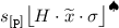• is a monitor where: $s_{[\mathtt {p} ]}$ is the indexed session being monitored; H is a local type with history (see below); $\widetilde{x}$ is a set of free variables; and the store $\sigma$ records their values. The tag $\spadesuit$ says whether the running process tied to the monitor is involved in a backward step ($\spadesuit = \blacklozenge$) or not ($\spadesuit = \lozenge$).

• is the message queue of session s, composed of an input part $h_i$ and an output part $h_o$. Messages sent by output prefixes are placed in the output part; an input prefix takes the first message in the output part and moves it to the input part. Hence, messages in the queue are not consumed but moved between the two parts of the queue.

• Finally, the running function serves to reverse the $\beta$-reduction resulting from the application $V\, {u}$. In , $\ell$ is the location where the application resides, and k is a freshly generated identifier.

These intuitions are formalized by the operational semantics of the MP model, which we do not discuss here; see Mezzina and Pérez’s papers [6, 7] for details.

2.3 Global and Local Types

As mentioned above, multiparty protocols are expressed as global types ($G, G', \ldots$), which can be projected onto local types ($T, T', \ldots$), one per participant. The syntax of value, global, and local types follows [3]:

Value types U include first-order values, and type $T\! \rightarrow \! \diamond$ for higher-order values: abstractions from names to processes (where $\diamond$ denotes the type of processes).

Global type $\mathtt {p}\rightarrow \mathtt {q}:\langle U\rangle .G$ says that $\mathtt {p}$ sends a value of type U to $\mathtt {q}$, and then continues as G. Given a finite index set I and pairwise different labels $l_i$, global type $\mathtt {p}\rightarrow \mathtt {q}:\{l_i:G_i\}_{i \in I}$ specifies that $\mathtt {p}$ may choose label $l_i$, send this selection to $\mathtt {q}$, and then continue as $G_i$. In both cases, $\mathtt {p} \ne \mathtt {q}$. Recursive and terminated protocols are denoted $\mu X. G$ and $\mathtt {end}$, respectively.

Global types are sequential, but may describe implicit parallelism. As a simple example, the global type $G = \mathtt {p}\rightarrow \mathtt {q}:\langle \mathtt {bool}\rangle .\mathtt {r}\rightarrow \mathtt {s}:\langle \mathtt {nat}\rangle .\mathtt {end}$ is defined sequentially, but describes two independent exchanges (one involving $\mathtt {p}$ and $\mathtt {q}$, the other involving $\mathtt {r}$ and $\mathtt {s}$) which could be implemented in parallel. In this line, G may be regarded to be equivalent to $G' = \mathtt {r}\rightarrow \mathtt {s}:\langle \mathtt {nat}\rangle .\mathtt {p}\rightarrow \mathtt {q}:\langle \mathtt {bool}\rangle .\mathtt {end}$.

Local types are used in the monitors introduced above. Local types $\mathtt {p}!\langle U\rangle .T$ and $\mathtt {p}?\langle U\rangle .T$ denote, respectively, an output and input of value of type U by $\mathtt {p}$. Type $\mathtt {p} \& \{l_i: T_i\}_{i \in I}$ says that $\mathtt {p}$ offers different labeled alternatives; conversely, type $\mathtt {\mathtt {p}}\!\oplus \!\{l_i: T_i\}_{i \in I}$ says that $\mathtt {p}$ may select one of such alternatives. Recursive and terminated local types are denoted $\mu X. T$ and $\mathsf {end}$, respectively.

A distinguishing feature of the MP model are local types with history ($H, H'$). A type H is a local type equipped with a cursor (denoted ) used to distinguish the protocol actions that have been already executed (the past of the protocol) from those that are yet to be performed (the future of the protocol).

2.4 Projection

The projection of a global type G onto a participant $\mathtt {p}$, denoted $G\!\downarrow _{\mathtt {p}}$, is defined in Fig. 2. The definition is self-explanatory, perhaps except for choice. Intuitively, projection ensures that a choice between $\mathtt {p}$ and $\mathtt {q}$ should not implicitly determine different behavior for participants different from $\mathtt {p}$ and $\mathtt {q}$, for which any different behavior should be determined by some explicit communication. This is a condition adopted by the MP model but also by several other works, as it ensures decentralized implementability of multiparty session types. Our implementation relies on broadcasts to communicate choices to all protocol participants; this reduces the need for explicit communications in global types. Projection consistently handles the combination of recursion and choices in global types. In the particular case in which a branch of a choice in the global type may recurse back to the beginning, the local types for all involved participants will be themselves recursive; this ensures that participants will jump back to the beginning of the protocol in a coordinated way.

Fig. 2.

Projection of a global type G onto a participant $\mathtt {r}$ [6, 7].

2.5 Example: Three-Buyer Protocol

We illustrate the forward and backward reduction semantics, denoted and . To this end, we recall the running example by Mezzina and Pérez [7], namely a reversible variant of the Three-Buyer protocol (cf., e.g., [1]) with abstraction passing (delegation).

The Protocol as Global and Local Types. The protocol involves three buyers (Alice ($\mathtt {A}$), Bob ($\mathtt {B}$), and Carol ($\mathtt {C}$)) who interact with a Vendor ($\mathtt {V}$) as follows:

• 1. Alice sends a book title to Vendor, which replies back to Alice and Bob with a quote. Alice tells Bob how much she can contribute.

• 2. Bob notifies Vendor and Alice that he agrees with the price, and asks Carol to assist him in completing the protocol. To delegate his remaining interactions with Alice and Vendor to Carol, Bob sends her the code she must execute.

• 3. Carol continues the rest of the protocol with Vendor and Alice as if she were Bob. She sends Bob’s address (contained in the code she received) to Vendor.

• 4. Vendor answers to Alice and Carol (representing Bob) with the delivery date.

This protocol may be formalized as the following global type G:

Above, stands for (and similarly for local types). We write to denote the type $\mathsf {end}\! \rightarrow \! \diamond$, associated to a thunk $\lambda x.\,P$ with $x \not \in \mathtt {fn}(P)$, written $\{\!\{P\}\!\}$. A thunk is an inactive process, which is activated by applying to it a dummy name of type $\mathsf {end}$, denoted $*$. Also, $\mathsf {price}$ and $\mathsf {share}$ are base types treated as integers; $\mathsf {title}$, $\mathsf {OK}$, $\mathsf {address}$, and $\mathsf {date}$ are base types treated as strings. The projections of G onto local types are as follows:

Process Implementations and Their Behavior. We now give processes for each participant:

$$\begin{aligned} \text {Vendor}&= d !\langle x{\,:\,}G\!\downarrow _{\mathtt {V}} \rangle .x ?(t) .x !\langle price(t) \rangle .x !\langle price(t) \rangle . x ?(ok) .x ?(a) . x !\langle date \rangle .\mathbf {0}\\ \text {Alice}&= d ?(y{\,:\,}G\!\downarrow _{\mathtt {A}}) .y !\langle \text {`Logicomix'} \rangle .y ?(p) .y !\langle h \rangle .y ?(ok) .\mathbf {0}\\ \text {Bob}&= d ?(z{\,:\,}G\!\downarrow _{\mathtt {B}}) .z ?(p) .z ?(h) .z !\langle ok \rangle .z !\langle ok \rangle .z !\langle h \rangle . z !\big \langle \{\!\{z !\langle \text {`9747'} \rangle .z ?(d) .\mathbf {0}\}\!\} \big \rangle .\mathbf {0}\\ \text {Carol}&= d ?(w{\,:\,}G\!\downarrow _{\mathtt {C}}) .w ?(h) .w ?(code) .(code\, {*}) \end{aligned}$$

where $price(\cdot )$ returns a value of type $\mathsf {price}$ given a $\mathsf {title}$. Observe how Bob’s implementation sends part of its protocol to Carol as a thunk. The whole system, given below, is obtained by placing these processes in locations $\ell _1, \ldots , \ell _4$:

$$ M = \ell _1\left\{ \text {Vendor}\right\} \parallel \ell _2\left\{ \text {Alice}\right\} \parallel \ell _3\left\{ \text {Bob}\right\} \parallel \ell _4\left\{ \text {Carol}\right\} $$

We now use configuration M to discuss the reduction relations and ; below we shall refer to forward and backward reduction rules defined in Mezzina and Pérez’s paper [7, Sect. 2.2.2].

From M, the session starts with an application of Rule  , which defines a forward reduction that, by means of a synchronization on shared name d, initializes the protocol by creating running processes and monitors:

where , , , and stand for the continuation of processes $\text {Vendor}$, $\text {Alice}$, $\text {Bob}$, and $\text {Carol}$ after the service request/accept. Observe that s is a fresh session name created after initialization; we write to denote a substitution of variable x with session name $s_{[\mathtt {V}]}$.

From $M_1$ we could either undo this forward reduction (using Rule  ) or execute the communication from $\text {Alice}$ to $\text {Vendor}$, using Rules  and  as follows:

where $N_2$ stands for processes/monitors for Vendor, Bob, and Carol (not involved in the reduction). In $M_2$, the message from $\mathtt {A}$ to $\mathtt {V}$ now appears in the output part of the queue. An additional forward step completes the synchronization:

where $\sigma _3 = [x\mapsto d],[t\mapsto \text {`Logicomix'}]$, $T_\mathsf {\mathtt {V}} = \mathtt {B}?\langle \mathsf {OK}\rangle .\mathtt {B}?\langle \mathsf {address}\rangle .\mathtt {B}!\langle \mathsf {date}\rangle .\mathsf {end}$, and $N_3$ stands for the rest of the system. Note that the cursors () in the local types with history of the monitors $s_{[\mathtt {V} ]}$ and $s_{[\mathtt {A} ]}$ have moved; also, the message from $\mathtt {A}$ to $\mathtt {V}$ is now in the input part of the queue.

We now illustrate reversibility: to return to $M_1$ from $M_3$ we need three backward reduction rules: , , and . First, Rule  modifies the tags of monitors $s_{[\mathtt {V} ]}$ and $s_{[\mathtt {A} ]}$, from $\lozenge$ to :

where is a type context (with hole $\bullet$) and, as before, $N_4$ represents the rest of the system.

$M_4$ has several possible forward and backward reductions. One particular backward reduction is the one that uses Rule  to undo the input at $\mathtt {V}$:

As a result, the message from $\mathtt {A}$ to $\mathtt {V}$ is back again in the output part of the queue. The following backward reduction uses Rule  to undo the output at $\mathtt {A}$:

Clearly, $M_6 = M_1$. Summing up, the forward reductions can be reversed by the backward reductions .

Abstraction Passing (Delegation). To illustrate abstraction passing, let us assume that $M_3$ above performs forward reductions until the configuration:

where $\{\!\{s_{[\mathtt {B}]} !\langle \text {`9747'} \rangle .s_{[\mathtt {B}]} ?(d) .\mathbf {0}\}\!\}$ is a thunk (to be activated with the dummy value $*$) and , $\sigma _7$, , $\sigma _8$, and $h_7$ capture past interactions as follows:

If to enable a (forward) synchronization we would have:

where $\sigma _9 = \sigma _8 [code\mapsto \{\!\{s_{[\mathtt {B}]} !\langle \text {`9747'} \rangle .s_{[\mathtt {B}]} ?(d) .\mathbf {0}\}\!\}]$. We now may obtain the actual code sent from $\mathtt {B}$ to $\mathtt {C}$:

where $N_6$ is the rest of the system. Notice that this reduction has added a running function on a fresh k, which is also used in the type stored in the monitor $s_{[\mathtt {C} ]}$.

The reduction completes the code mobility from $\mathtt {B}$ to $\mathtt {C}$: the now active thunk will execute $\mathtt {B}$’s protocol from $\mathtt {C}$’s location. Observe that Bob’s identity $\mathtt {B}$ is “hardwired” in the sent thunk; there is no way for $\mathtt {C}$ to execute the code by referring to a participant different from $\mathtt {B}$.

3 Implementing the MP Model in Haskell

We represent the process calculus, global types, local types, and the information for reversal as syntax trees. Local types are obtained by from the global type via projection, which we implement following Sect. 2.4, whereas processes and global types are written by the programmer. For this reason, we want to provide a convenient way to specify them as domain-specific languages (DSLs).

3.1 DSLs with the Free Monad

Free monads are a common way of defining DSLs in Haskell, mainly because they allow the use of do-notation to write programs in the DSL.

A simple practical example is a stack-based calculator:

We define a data type with our instructions, and make sure it has a Functor instance (i.e., there exists a function ). This instance is automatically derived using the DeriveFunctor language extension. Given an instance of Functor, Free returns the free monad on that functor. In this example, the free monad on Operation describes a list of instructions.

In general, a value of type ‘Free Operation a’ describes a program with holes: an incomplete program with placeholder values of type a in the position of some continuations. Composition allows filling in the holes with (possibly incomplete) subprograms. The holes are places where the Pure constructor occurs in the program. When evaluating, we want to have a tree without holes. We can leverage the type system to guarantee that Pure does not occur in the programs we evaluate by using Void.

Void is the data type with zero values (similar to the empty set). Thus, a value of the type Free Operation Void cannot be of the shape Pure _, because it requires a value of type Void. An alternative approach is to use existential quantification, which requires enabling a language extension.

We define wrappers around the constructors for convenience. The liftF function takes a concrete value of our program functor (ProgramF a) and turns it into a free value (Free ProgramF a, i.e., Program a). The helpers are used to write programs with do-notation:

Finally, we expose a function to evaluate the structure (but only if it is finite). Typically, a Free monad is transformed into some other monad, which in turn is evaluated. Here we can first transform into State, and then evaluate that.

3.2 Implementing Processes

The implementation uses an algebraic data type to encode all the process constructors in the process syntax of P given in Sect. 2.2. Apart from the process-level recursion, Program is a direct translation of that process syntax:

As already discussed, processes exchange values. With respect to the syntax of values V, W discussed in Sect. 2.2, the Value type, given below, has some extra constructors which allow us to write more interesting examples: we have added integers, strings, and basic integer and comparison operators. We use VReference to denote the variables present in the formal syntax for V. The Value type also includes the label used to differentiate the different cases of offer and select statements.

We need some extra concepts to actually write programs with this syntax.

Delegation via Abstraction Passing. Delegation occurs when a participant can send (part of) its protocol to be fulfilled (i.e., implemented) by another participant. This mechanism was illustrated in the example in Sect. 2.5, where Carol acts on behalf of Bob by receiving and executing his code. For further illustration of the convenience of this mechanism, consider a load balancing server: from the client’s perspective, the server handles the request, but actually the load balancer delegates incoming requests to workers. The client does not need to be aware of this implementation detail. Recall the definition of ProgramF, given just above:

The ProgramF constructors that move the local type forward (send/receive, select/offer) have an owner field that stores whose local type they should be checked against and modify. In the formal definition of the MP model, the connection between local types and processes/participants is enforced by the operational semantics. The owner field is also present in TypeContext, the data type we define for representing local types in Sect. 3.4.

As explained in Sect. 2.2, each protocol participant has its own monitor with its own store. Because these stores are not shared, all variables occurring in the arguments to operators and in function bodies must be dereferenced before a value can be safely sent over a channel.

A Convenient DSL. Many of the ProgramF constructors require an owner; we can thread the owner through a block with a wrapper around Free. We use StateT containing the owner and a counter to generate unique variable names.

We can now implement the Vendor from the three-buyer example as:

3.3 Global Types

Following Fig. 1, our implementation uses a global type specification to obtain a local type (of type LocalType), one per participant, by means of projection. This is implemented as described in Sect. 2.4. Much like the process syntax, the specification of the global types discussed in Sect. 2.3 closely mimics the formal definition:

where we use ‘tipe’ because ‘type’ is a reserved keyword in Haskell.

Constructors RecursionPoint, RecursionVariable, and WeakenRecursion are required to support nested recursion; they are taken from van Walree’s work [10]. A RecursionPoint is a point in the protocol to which we can jump back later. A RecursionVariable triggers jumping to a previously encountered RecursionPoint. By default, it will jump to the closest and most recently encountered RecursionPoint, but WeakenRecursion makes it jump one RecursionPoint higher; encountering two weakens will jump two levels higher, etc.

We use Monad.Free to build a DSL for defining global types:

Example 1

(Nested Recursion). The snippet below illustrates nested recursion. There is an outer loop that will perform a piece of protocol or end, and an inner loop that sends messages from A to B. When the inner loop is done, control flow returns to the outer loop:

Similarly, the global type for three-buyer example (cf. Sect. 2.5) can be written as:

3.4 A Reversible Semantics

Having shown implementations for processes and global types, we now explain how to implement the reversible operational semantics for the MP model, which was illustrated in Sect. 2.5. We should define structures that allow us to move back to prior program states, reversing forward steps.

To enable backward steps, we need to store some information when we move forward, just as enabled by the configurations in the MP model (cf. Sect. 2.2). Indeed, we need to track information about the local type and the process. To implement local types with history, we define a data type called TypeContext: it contains the actions that have been performed; for some of them, it also stores extra information (e.g., owner). For the process, we need to track four things:

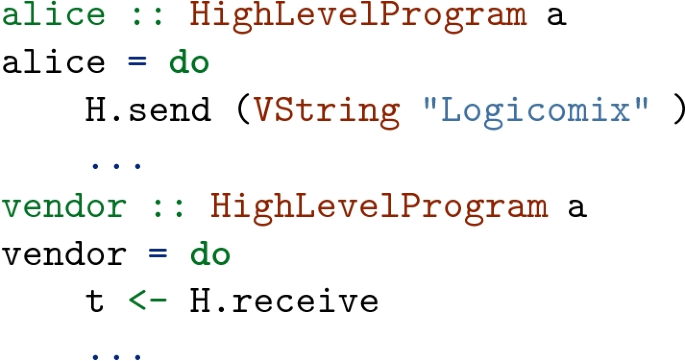
• 1. Used variable names in receives. Recall the process implementation for the vendor in the three-buyer example in Sect. 2.5:

  $$\begin{aligned} \text {Vendor}&= d !\langle x:G\!\downarrow _{\mathtt {V}} \rangle .x ?(t) .x !\langle price(t) \rangle .x !\langle price(t) \rangle . x ?(ok) .x ?(a) . x !\langle date \rangle .\mathbf {0}\end{aligned}$$

  We can implement this process as:

  

  The rest of the program depends on the assigned name. So, e.g., when we evaluate the line (moving to configuration $M_3$, cf. Sect. 2.5), and then revert it, we must reconstruct a receive that assigns to t, because the following lines depend on name t.

• 2. Function calls and their arguments. Consider the reduction from configuration $M_7$ to $M_8$, as discussed in Sect. 2.5. Once the thunk is evaluated, producing configuration $M_8$, we lose all evidence that the code produced by the evaluation resulted from a function application. Without this evidence, reversing $M_8$ will not result in $M_7$. Indeed, we need to keep track of function applications. Following the semantics of the MP model, the function and its argument are stored in a map indexed by a unique identifier k. The identifier k itself is also stored in the local type with history to later associate the type with a specific function and argument. The reduction from $M_8$ to $M_9$, discussed in Sect. 2.5, offers an example of this tracking mechanism in the formal model.

  Notice that a stack would seem a simpler solution, but it can give invalid behavior. Say that a participant is running in two locations, and the last-performed action at both locations is a function application. Now we want to undo both applications, but the order in which to undo them is undefined: we need both orders to work. Only using a stack could mix up the applications. When the application keeps track of exactly which function and argument it used the end result is always the same.

• 3. Messages on the channel. We consider again the implementation of the first three steps of the protocol:

  

  After Alice sends her message, it has to be stored to successfully undo the sending action. Likewise, when starting from configuration $M_3$ and undoing the receive, the value must be placed back into the queue.

  Our implementation closely follows the formal semantics of the MP model. As discussed in Sect. 2.2, the message queue has an input and an output part. This allows to describe how a message moves from the sender into the output queue. Reception is represented by moving the message to the input queue, which serves as a history stack. When the receive is reversed, the queue pops the message from its stack and puts it at the output queue again. Reversing the send moves the message from the output queue back to the sender’s program.

• 4. Unused branches. When a labeled choice is made and then reverted, we want all our options to be available again. In the MP model, choices made so far are stored in a stack denoted $\mathtt {C}$, inside a running process (cf. Sect. 2.2).

  The following code shows how we store these choices:

  

  We need to remember which choice was made; the order of the options is important. We use a Zipper to store the elements in order and use the central ‘a’ to store the choice that was made.

3.5 Putting It All Together

With all the definitions in place, we can now define the forward and backward evaluation of our system. The reduction relations and , discussed and illustrated in Sect. 2.5, are implemented with the types:

These functions take a Location (the analogue of the locations $\ell$ in the formal model) and try to move the process at that location forward or backward. The Session type contains the ExecutionState, the state of the session (all programs, local types, variable bindings, etc.). The Except type indicates that errors of type Error can be thrown (e.g., when an unbound variable is used):

The configurations of the MP model (cf. Sect. 2.2) are our main reference to store the execution state. Some data is bound to its location (e.g., the current running process), while other data is bound to its participant (e.g., the local type). The information about a participant is grouped in a type called Monitor:

Some explanations follow:

• _localType contains TypeContext and LocalType stored as a tuple. This tuple gives a cursor into the local type, where everything to the left is the past and everything to the right is the future.

• The next two fields keep track of recursion in the local type. We use the _recursiveVariableNumber is an index into the _recursionPoints list: when a RecursionVariable is encountered we look at that index to find the new future local type.

• _usedVariables and _applicationHistory are used in reversal. As mentioned in Sect. 3.4, used variable names must be stored so we can use them when reversing. We store them in a stack keeping both the original name given by the programmer and the generated unique internal name. For function applications we use a Map indexed by unique identifiers that stores function and argument.

• _store is a variable store with the currently defined bindings. Variable shadowing (when two processes of the same participant define the same variable name) is not an issue: variables are assigned a name that is guaranteed unique.

We can now define ExecutionState: it contains some counters for generating unique variable names, a monitor for every participant, and a program for every location. Additionally, every location has a default participant and a stack for unchosen branches:

The message queue is global and thus also lives in the ExecutionState. Finally, we need a way of inspecting values, to see whether they are functions and if so, to extract their bodies for application.

3.6 Causal Consistency?

As mentioned in Sect. 1, causal consistency is a key correctness criterion for a reversible semantics: this property ensures that backward steps always lead to states that could have been reached by moving forward only. The global type defines a partial order on all the communication steps. The relation of this partial order is a causal dependency. Stepping backward is only allowed when all its causally dependent actions are undone.

The reversible semantics of the MP model, summarized in Sect. 2, enjoys causal consistency for processes running a single global protocol (i.e., a single session). Rather than typed processes, the MP model describes untyped processes whose (reversible) operational semantics is governed by local types. This suffices to prove causal consistency, but also to ensure that process reductions correspond to valid actions specified by the global type. Given this, one may then wonder, does our Haskell implementation preserve causal consistency?

In the semantics and the implementation, this causal dependency becomes a data dependency. For instance, a send can only be undone only when the queue is in a state that can only be reached by first undoing the corresponding receive. Only in this state is the appropriate data of the appropriate type available. Being able to undo a send thus means that the corresponding receive has already been reversed, so it is impossible to introduce causal inconsistencies.

Because of the encoding of causal dependencies as data dependencies, and the fact that these data dependencies are preserved in the implementation, we claim that our Haskell implementation respects the formal semantics of the MP model, and therefore that it preserves the causal consistency property.

4 Running and Debugging Programs

Finally, we want to be able to run our programs. Our implementation offers mechanisms to step through a program interactively, and run it to completion.

We can step through the program interactively in the Haskell REPL environment. When the ThreeBuyer example is loaded, the program is in a state corresponding to configuration $M_1$ from Sect. 2.5. We can print the initial state of our program:

Next we introduce the stepForward and stepBackward functions. They use mutability, normally frowned upon in Haskell, to avoid having to manually keep track of the updated program state like in the snippet below:

Manual state passing is error-prone and inconvenient. We provide helpers to work around this issue (internally, those helpers use IORef). We must first initialize the program state:

We can then use stepForward and stepBackward to evaluate the program: we advance Alice at $l_1$ to reach $M_2$ and then the vendor at $l_4$ to reach $M_3$:

When the user tries an invalid step, an error is displayed. For instance, in state $M_3$, where $l_1$ and $l_4$ have been moved forward once (like in the snippet above), $l_1$ cannot move forward (it needs to receive but there is nothing in the queue) and not backward ($l_4$, the receiver, must undo its action first).

Errors are defined as:

To fully evaluate a program, we use a round-robin scheduler that calls forward on the locations in order. A forward step can produce an error. There are two error cases that we can recover from:

• blocked on receive, either QueueError _ InvalidQueueItem or QueueError _ EmptyQueue: the process wants to perform a receive, but the expected item is not at the top of the queue yet. In this case we proceed evaluating the other locations so they can send the value that the faulty location expects. Above, ‘_’ means that we ignore the String field used to provide better error messages. Because no error message is generated, that field is not needed.

• location terminates with Terminated: the execution has reached a NoOp. In this case we do not want to schedule this location any more.

Otherwise we continue until there are no active (non-terminated) locations left.

Running until completion (or error) is also available in the REPL:

Note that this scheduler can still get into deadlocks, for instance consider these two equivalent global types:

Above, the second and third messages (involving ) are swapped. The communication they describe is the same, but in practice they are very different. The first example will run to completion, whereas the second can deadlock because A can send a Share before V sends the Price. B expects the price from V first, but the share from A is the first in the queue. Therefore, no progress can be made.

In general, a key issue is that a global type is written sequentially, while it may represent implicit parallelism, as explained in Sect. 2.3. Currently, our implementation just executes the global type with the order given by the programmer. It should be possible to execute communication actions in different but equivalent orders; these optimizations are beyond the scope of our current implementation.

5 Discussion and Concluding Remarks

5.1 Benefits of Pure Functional Programming

It has consistently been the case that sticking closer to the formal model gives better code. The abilities that Haskell gives for directly specifying formal statements are invaluable. A key invaluable feature is algebraic data types (ADTs, also known as tagged unions or sum types). Compare the formal definition given in Sect. 2.3 and the Haskell data type for global types.

The definitions correspond almost directly: the WeakenRecursion constructor is added to support nested recursion, which the formal model does not explicitly represent. Moreover, we know that these are all the ways to construct a value of type GlobalTypeF and can exhaustively match on all the cases. Functional languages have had these features for a very long time. Secondly, purity and immutability are very useful in implementing and testing the reversible semantics.

In a pure language, given functions and to prove that $f$ and $g$ are inverses it is enough to prove that $\mathtt {f} \cdot \mathtt {g}$ and $\mathtt {g} \cdot \mathtt {f}$ both compose to the identity. In an impure language, even if these equalities are observed we cannot be sure that there were no side-effects. Because we do not need to consider a context (the outside world) in a pure language, checking that reversibility works is as simple as comparing initial and final states for all backward reduction rules.

5.2 Concluding Remarks

We presented a functional implementation of the (reversible) MP model [7] using Haskell. By embedding this reversible semantics we can now execute our example programs automatically and inspect them interactively.

We have seen that the MP model can be split into three core components: (i) a process calculus, (ii) multiparty session types (global and local types), and (iii) forward and backward reduction semantics. The three components can be cleanly represented as recursive Haskell data types. We are confident that other features developed in Mezzina and Pérez’s work [7] (in particular, an alternative semantics for decoupled rollbacks) can easily be integrated in the development described here. Relatedly, the implementation process has shown that sticking to the formal model leads to better code; there is less space for bugs to creep in. Furthermore, Haskell’s mathematical nature means that the implementation inspired by the formal specification is easy (and often idiomatic) to express. Finally, we have discussed how Haskell allows for the definition of flexible embedded domain-specific languages, and makes it easy to transform between different representations of our programs (using among others Monad.Free).

References

Coppo, M., Dezani-Ciancaglini, M., Padovani, L., Yoshida, N.: A gentle introduction to multiparty asynchronous session types. In: Bernardo, M., Johnsen, E.B. (eds.) SFM 2015. LNCS, vol. 9104, pp. 146–178. Springer, Cham (2015). https://doi.org/10.1007/978-3-319-18941-3_4. http://www.di.unito.it/~dezani/papers/cdpy15.pdf
Honda, K., Vasconcelos, V.T., Kubo, M.: Language primitives and type discipline for structured communication-based programming. In: Hankin, C. (ed.) ESOP 1998. LNCS, vol. 1381, pp. 122–138. Springer, Heidelberg (1998). https://doi.org/10.1007/BFb0053567
Honda, K., Yoshida, N., Carbone, M.: Multiparty asynchronous session types. In: Necula, G.C., Wadler, P. (eds.) POPL 2008, pp. 273–284. ACM (2008). https://doi.org/10.1145/1328438.1328472
Kouzapas, D., Pérez, J.A., Yoshida, N.: On the relative expressiveness of higher-order session processes. In: Thiemann, P. (ed.) ESOP 2016. LNCS, vol. 9632, pp. 446–475. Springer, Heidelberg (2016). https://doi.org/10.1007/978-3-662-49498-1_18
Lanese, I., Mezzina, C.A., Tiezzi, F.: Causal-consistent reversibility. Bull. EATCS 114 (2014). http://eatcs.org/beatcs/index.php/beatcs/article/view/305
Mezzina, C.A., Pérez, J.A.: Causally consistent reversible choreographies. CoRR abs/1703.06021 (2017). http://arxiv.org/abs/1703.06021
Mezzina, C.A., Pérez, J.A.: Causally consistent reversible choreographies: a monitors-as-memories approach. In: Vanhoof, W., Pientka, B. (eds.) Proceedings of the 19th International Symposium on Principles and Practice of Declarative Programming, Namur, Belgium, 09–11 October 2017, pp. 127–138. ACM (2017). https://doi.org/10.1145/3131851.3131864
Milner, R., Parrow, J., Walker, D.: A calculus of mobile processes, parts I and II. Inf. Comput. 100(1), 1–40 (1992)
Sangiorgi, D.: Asynchronous process calculi: the first-and higher-order paradigms. Theor. Comput. Sci. 253(2), 311–350 (2001). https://doi.org/10.1016/S0304-3975(00)00097-9
van Walree, F.: Session types in Cloud Haskell. Master’s thesis, University of Utrecht (2017). https://dspace.library.uu.nl/handle/1874/355676
Acknowledgments
Many thanks to the anonymous reviewers and to the TFP’18 co-chairs (Michał Pałka and Magnus Myreen) for their useful remarks and suggestions, which led to substantial improvements. Pérez is also affiliated to CWI, Amsterdam, The Netherlands and to the NOVA Laboratory for Computer Science and Informatics (supported by FCT grant NOVA LINCS PEst/UID/CEC/04516/2013), Universidade Nova de Lisboa, Portugal.
This research has been partially supported by the Undergraduate School of Science and the Bernoulli Institute of the University of Groningen. We also acknowledge support from the COST Action IC1405 “Reversible computation – Extending horizons of computing”.
Author information
Authors and Affiliations
Corresponding author
Editor information
Editors and Affiliations
Rights and permissions
Copyright information
© 2019 Springer Nature Switzerland AG
About this paper
Cite this paper
de Vries, F., Pérez, J.A. (2019). Reversible Session-Based Concurrency in Haskell. In: Pałka, M., Myreen, M. (eds) Trends in Functional Programming. TFP 2018. Lecture Notes in Computer Science(), vol 11457. Springer, Cham. https://doi.org/10.1007/978-3-030-18506-0_2
Download citation
DOI: https://doi.org/10.1007/978-3-030-18506-0_2
Published:
Publisher Name: Springer, Cham
Print ISBN: 978-3-030-18505-3
Online ISBN: 978-3-030-18506-0
eBook Packages: Computer ScienceComputer Science (R0)