
Abstract
Simulation and valuation of finance instruments require numbers with specified distributions. For example, in Sect. 1.6 we have used numbers Z drawn from a standard normal distribution, \(Z \sim \mathcal{N}(0,1)\). If possible the numbers should be random. But the generation of “random numbers” by digital computers, after all, is done in a deterministic and entirely predictable way. If this point is to be stressed, one uses the term pseudo-random.
Access provided by CONRICYT-eBooks. Download chapter PDF
Simulation and valuation of finance instruments require numbers with specified distributions. For example, in Sect. 1.6 we have used numbers Z drawn from a standard normal distribution, \(Z \sim \mathcal{N}(0,1)\). If possible the numbers should be random. But the generation of “random numbers” by digital computers, after all, is done in a deterministic and entirely predictable way. If this point is to be stressed, one uses the term pseudo-random.Footnote 1
Computer-generated random numbers mimic the properties of true random numbers as much as possible. This is discussed for uniformly distributed random numbers in Sect. 2.1. Suitable transformations or rejection methods generate samples from other distributions, in particular, normally distributed numbers (Sects. 2.2 and 2.3). Section 2.3 includes the vector case, where normally distributed numbers are calculated with prescribed correlation.
Another approach is to dispense with randomness and to generate quasi-random numbers, which aim at avoiding one disadvantage of random numbers, namely, the potential lack of equidistributedness. The resulting low-discrepancy numbers will be discussed in Sect. 2.5. These numbers are used for the deterministic Monte Carlo integration (Sect. 2.4).
A sequence of numbers is called a sample from F if the numbers are independent realizations of a random variable with distribution function F.
If F is the uniform distribution over the interval [0, 1], then we call the samples from F uniform deviates (variates), notation \(\sim \mathcal{U}[0,1]\). If F is the standard normal distribution then we call the samples from F standard normal deviates (variates); as notation we use \(\sim \mathcal{N}(0,1)\). The basis of random-number generation is to draw uniform deviates.
2.1 Uniform Deviates
A standard approach to calculate uniform deviates is provided by linear congruential generators. We concentrate on algorithms that are easy to implement and ready for experiments.
2.1.1 Linear Congruential Generators
Choose integers M, a, b, with a, b < M, a ≠ 0. For an integer N 0 a sequence of integers N i is defined by
Algorithm 2.2 (Linear Congruential Generator)
-
Choose N 0 .
-
For i = 1, 2, … calculate
$$\displaystyle{ N_{i} = (aN_{i-1} + b)\ \mbox{ mod }M\,. }$$(2.1)
The modulo congruence N = Y mod M between two numbers N and Y is an equivalence relation [147]. The initial integer N 0 is called the seed. Numbers U i ∈ [0, 1) are defined by
and will be taken as uniform deviates. Whether the numbers U i or N i are suitable will depend on the choice of M, a, b and will be discussed next.
Properties 2.3 (Periodicity)
-
(a)
N i ∈ {0, 1, …, M − 1}
-
(b)
The N i are periodic with period ≤ M.
(Because there are not M + 1 different N i . So two in {N 0, …, N M } must be equal, N i = N i+p with p ≤ M.)
Obviously, some peculiarities must be excluded. For example, N = 0 must be ruled out in case b = 0, because otherwise N i = 0 would repeat. In case a = 1 the generator settles down to N n = (N 0 + nb) mod M. This sequence is predictable too easily. Various other properties and requirements are discussed in the literature, in particular in [226]. In case the period is M, the numbers U i are distributed “evenly” when exactly M numbers are needed. Then each grid point on a mesh on [0,1] with mesh size \(\frac{1} {M}\) is occupied once.
After these observations we start searching for good choices of M, a, b. There are numerous possible choices with bad properties. For serious computations we recommend to rely on suggestions of the literature. Press et al. [306] presents a table of “quick and dirty” generators, for example, M = 244, 944, a = 1597, b = 51, 749. Criteria are needed to decide which of the many possible generators are recommendable.
2.1.2 Quality of Generators
What are good random numbers? A practical answer is the requirement that the numbers should meet “all” aims, or rather pass as many tests as possible. The requirements on good number generators can roughly be divided into three groups.
The first requirement is that of a large period. In view of Property 2.3 the number M must be as large as possible, because a small set of numbers makes the outcome easier to predict—a contrast to randomness. This leads to select M close to the largest integer machine number. But a period p close to M is only achieved if a and b are chosen properly. Criteria for relations among M, p, a, b have been derived by number-theoretic arguments. This is outlined in [226, 317]. For 32-bit computers, a common choice has been M = 231 − 1, a = 16807, b = 0.
A second group of requirements are statistical tests that check whether the numbers are distributed as intended. The simplest of such tests evaluates the sample mean \(\hat{\mu }\) and the sample variance \(\hat{s}^{2}\) (B.11) of the calculated random variates, and compares to the desired values of μ and σ 2. (Recall μ = 1∕2 and σ 2 = 1∕12 for the uniform distribution.) Another simple test is to check correlations. For example, it would not be desirable if small numbers are likely to be followed by small numbers.
A slightly more involved test checks how well the probability distribution is approximated. This works for general distributions ( → Exercise 2.1). Here we briefly summarize an approach for uniform deviates. Calculate j samples from a random number generator, and investigate how the samples distribute on the unit interval. To this end, divide the unit interval into subintervals of equal length ΔU, and denote by j k the number of samples that fall into the kth subinterval
Then j k ∕j should be close the desired probability, which for this setup is ΔU. Hence a plot of the quotients
against kΔU should be a good approximation of 1 [0,1], the density of the uniform distribution. This procedure is just the simplest test; for more ambitious tests, consult [226].
The third group of tests is to check how well the random numbers distribute in higher-dimensional spaces. This issue of the lattice structure is discussed next. We derive a priori analytical results on where the random numbers produced by Algorithm 2.2 are distributed.
2.1.3 Random Vectors and Lattice Structure
Random numbers N i can be arranged in m-tuples (N i , N i+1, …, N i+m−1) for i ≥ 1. Then the tuples or the corresponding points (U i , …, U i+m−1) ∈ [0, 1)m are analyzed with respect to correlation and distribution. The sequences defined by the generator of Algorithm 2.2 lie on (m − 1)-dimensional hyperplanes. This statement is trivial since it holds for the M parallel planes through U = i∕M, i = 0, …, M − 1 (any of the m components). But if all points fall on only a small number of parallel hyperplanes (with large empty gaps in between), then the generator would be impractical in many applications. Next we analyze the generator whether such unfavorable planes exist, restricting ourselves to the case m = 2.
For m = 2 the hyperplanes in (U i−1, U i )-space are straight lines, and are defined by z 0 U i−1 + z 1 U i = λ, with parameters z 0, z 1, λ. The modulus operation (2.1) can be written
k an integer, k = k(i). A side calculation for arbitrary z 0, z 1 shows
We divide by M and obtain the equation of a straight line in the (U i−1, U i )-plane, namely,
The points calculated by Algorithm 2.2 lie on these straight lines. To eliminate the seed we take i > 1. For each tuple (z 0, z 1), the Eq. (2.3) defines a family of parallel straight lines, one for each number out of the finite set of c’s. The question is whether there exists a tuple (z 0, z 1) such that only few of the straight lines cut the square [0, 1)2. In this case wide areas of the square would be free of random points, which violates the requirement of a “uniform” distribution of the points. The minimum number of parallel straight lines (hyperplanes) cutting the square, or equivalently the maximum distance between them, characterizes the worst case and serves as measure of the equidistributedness. Now we analyze the number of straight lines, searching for the worst case.
For analyzing the number of planes, the cardinality of the c matters. To find the worst case, restrict to integers (z 0, z 1) satisfying
Then the parameter c is integer. By solving (2.3) for c = z 0 U i−1 + z 1 U i − z 1 bM −1 and applying 0 ≤ U < 1 we obtain the maximal interval I c such that for each integer c ∈ I c its straight line cuts or touches the square [0, 1)2. Count how many such c’s exist, and there is the information we need. For some constellations of a, M, z 0 and z 1 it may be possible that the points (U i−1, U i ) lie on very few of these straight lines!
Example 2.4 (Academic Generator)
We discuss the generator
that is, the parameters are a = 2, b = 0, M = 11. The choice z 0 = −2, z 1 = 1 is one tuple satisfying (2.4), and the resulting family (2.3) of straight lines
in the (U i−1, U i )-plane is to be discussed. For U ∈ [0, 1) the inequality − 2 < c < 1 results. In view of (2.4) c is integer and so only the two integers c = −1 and c = 0 remain. The two corresponding straight lines cut the interior of [0, 1)2. As Fig. 2.1 illustrates, the points generated by the algorithm form a lattice. All points on the lattice lie on these two straight lines. The figure lets us discover also other parallel straight lines such that all points are caught (for other tuples z 0, z 1). The practical question is: What is the largest gap? ( → Exercise 2.2)

The points (U i−1, U i ) of Example 2.4
Example 2.5
N i = (1229N i−1 + 1) mod 2048
The requirement of Eq. (2.4)
is satisfied by z 0 = −1, z 1 = 5, because
For c from (2.3) and U i ∈ [0, 1) we have
Hence c ∈ {−1, 0, 1, 2, 3, 4}, and all points (U i−1, U i ) in [0, 1)2 lie on only six straight lines, see Fig. 2.2. On the “lowest” straight line (c = −1) there is only one point. The distance between straight lines measured along the vertical U i –axis is \(\frac{1} {z_{1}} = \frac{1} {5}\). Obviously, the (U i−1, U i )-points are by far not equidistributed on the square, although the positions U i appear uniformly distributed on the line.Footnote 2
Higher-dimensional vectors (m > 2) are analyzed analogously. The generator called RANDU
may serve as example. For m = 2 experiments show that the points (U i−1, U i ) are nicely equidistributed. But equidistribution for m = 2 does not imply equidistribution for larger m. Testing RANDU for m = 3 reveals a severe defect: Its random points in the cube [0, 1)3 fall on only 15 planes ( → Exercise 2.3 and Topic 14 in the Topics fCF).
In Example 2.4 we asked what the maximum gap between the parallel straight lines is. In other words, we have searched for stripes of maximum size in which no point (U i−1, U i ) falls. Alternatively one can directly analyze the lattice formed by consecutive points. For illustration consider again Fig. 2.1. We follow the points starting with \(( \frac{1} {11}, \frac{2} {11})\). By vectorwise adding an appropriate multiple of (1, a) = (1, 2) the next two points are obtained. Proceeding in this way one has to take care that upon leaving the unit square each component with value ≥ 1 must be reduced to [0, 1) to observe mod M. The reader may verify this with Example 2.4 and numerate the points of the lattice in Fig. 2.1 in the correct sequence. In this way the lattice can be defined. This process of defining the lattice can be generalized to higher dimensions m > 2. ( → Exercise 2.4) One aims at a good distribution of the points (U i , …, U i+m−1) for as many m are possible.
A disadvantage of the linear congruential generators of Algorithm 2.2 is the boundedness of the period by M and hence by the word length of the computer. The situation can be improved by shuffling the random numbers in a random way. For practical purposes, the period gets close enough to infinity. (The reader may test this on Example 2.5.) For practical advice we refer to [306].
2.1.4 Fibonacci Generators
The original Fibonacci recursion motivates trying the formula
It turns out that this first attempt of a three-term recursion is not suitable for generating random numbers ( → Exercise 2.5). The modified approach
for suitable integers ν, μ is called lagged Fibonacci generator. For many choices of ν, μ the approach (2.5) leads to acceptable generators. Kahaner et al. [210] recommends
Example 2.6 (Lagged Fibonacci Generator)
The recursion of Example 2.6 immediately produces floating-point numbers U i ∈ [0, 1). This generator requires a prologue in which 17 initial U’s are generated by means of another method. The core of the algorithm is
Algorithm 2.7 (Loop of a Fibonacci Generator)
-
Repeat:
-
ζ = U(i) − U( j) ,
-
if (ζ < 0), set ζ = ζ + 1 ,
-
U(i) = ζ ,
-
i = i − 1 ,
-
j = j − 1 ,
-
if i = 0, set i = 17 ,
-
if j = 0, set j = 17 .
Initialization: Set i = 17, j = 5, and calculate U 1, …, U 17 with a congruential generator, for instance with M = 714, 025, a = 1366, b = 150, 889. Set the seed N 0 equal to your favorite dream number, possibly inspired by the system clock of your computer.
Figure 2.3 depicts 10, 000 random points calculated by means of Algorithm 2.7. Visual inspection suggests that the points are not arranged in some apparent structure. The points appear to be sufficiently random. But the generator provided by Example 2.6 is not sophisticated enough for ambitious applications; its pseudo-random numbers are somewhat correlated.

Ten thousand (pseudo-)random points (U i−1, U i ), calculated with Algorithm 2.7
Section 2.1 has introduced some basic aspects of generating uniformly distributed random numbers. Professional algorithms also apply bit operations in the computer. A generator of uniform deviates that can be highly recommended is a Mersenne twister [264]. Its period is truly remarkable, and the points (U i , …, U i+m−1) are well distributed until high values of the dimension m.
2.2 Extending to Random Variables from Other Distributions
Frequently, normal variates are needed. Their generation is based on uniform deviates. The simplest strategy is to calculate
X has expectation 0 and variance 1. The central limit theorem ( → Appendix B) assures that X is approximately distributed normally ( → Exercise 2.6). But this crude attempt is not satisfying. Better methods calculate nonuniformly distributed random variables, for example, by a suitable transformation out of a uniformly distributed random variable [103]. But the most obvious approach inverts the distribution function.
2.2.1 Inversion
The following theorem is the basis for inversion methods.
Theorem 2.8 (Inversion)
Suppose \(U \sim \mathcal{U}[0,1]\) and F be a continuous strictly increasing distribution function. Then F −1(U) is a sample from F.
Proof
Let P denote the underlying probability.
\(U \sim \mathcal{U}[0,1]\) means P(U ≤ ξ) = ξ for 0 ≤ ξ ≤ 1.
Consequently
Application
Following Theorem 2.8, the inversion methodFootnote 3 generates uniform deviates \(u \sim \mathcal{U}[0,1]\) and sets x = F −1(u) ( → Exercises 2.7, 2.8, 2.9). There are some examples where the inverse is available analytically. For example, the distribution of the exponential distribution with parameter λ (below in Example 2.10) is F(x) = 1 − e−λx, and its inverse is \(F^{-1}(u) = -\frac{1} {\lambda } \log (1 - u)\). To judge the inversion method we consider the normal distribution as the most important example. Neither for its distribution function F nor for its inverse F −1 there is a closed-form expression ( → Exercise 5). So numerical methods are used. We discuss two approaches.
Numerical inversion means to calculate iteratively a solution x of the equation F(x) = u for prescribed u. In particular for the normal distribution, this iteration requires tricky termination criteria, in particular when x is large. Then we are in the situation u ≈ 1, where tiny changes in u lead to large changes in x (Fig. 2.4). An approximation of the solution x of F(x) − u = 0 can be calculated with bisection, or Newton’s method, or the secant method ( → Appendix C.1).

Normal distribution; small changes in u can lead to large changes in x
Alternatively the inversion x = F −1(u) can be approximated by a suitably constructed function G(u) with
Then only x = G(u) needs to be evaluated. Constructing such an approximation formula G, it is important to realize that F −1(u) has “vertical” tangents at u = 1 (horizontal in Fig. 2.4). The pole behavior must be reproduced correctly by an approximating function G. This suggests to use rational approximation ( → Appendix C.1). For the Gaussian distribution one incorporates the point symmetry with respect to \((u,x) = (\frac{1} {2},0)\), and the pole at u = 1 (and hence at u = 0) in the ansatz for G ( → Exercise 2.10). Rational approximation of F −1(u) with a sufficiently large number of terms leads to high accuracy [278]. The formulas are given in Appendix E.2.
2.2.2 Transformation in ℝ1
Another class of methods uses transformations between random variables. We start the discussion with the scalar case. If we have a random variable X with known density and distribution, what can we say about the density and distribution of a transformed h(X)?
Theorem 2.9 (Transformation in Scalar Case)
Suppose X is a random variable with density f(x) and distribution F(x). Further assume h: S → B with \(S,B \subseteq \mathbb{R}\) , where S is the support Footnote 4 of f(x), and let h be strictly monotonic.
-
(a)
Then Y: = h(X) is a random variable. Its distribution F Y is
$$\displaystyle\begin{array}{rcl} F_{Y }(\,y)& =& F(h^{-1}(\,y))\quad \mathit{\mbox{ in case }}h^{{\prime}} > 0\,, {}\\ F_{Y }(\,y)& =& 1 - F(h^{-1}(\,y))\quad \mathit{\mbox{ in case }}h^{{\prime}} < 0\,. {}\\ \end{array}$$ -
(b)
If h −1 is absolutely continuous then for almost all y the density of h(X) is
$$\displaystyle{ f(h^{-1}(\,y))\left \vert \frac{\,\mathrm{d}h^{-1}(\,y)} {\,\mathrm{d}y} \right \vert \,. }$$(2.6)
Proof
-
(a)
For h ′ > 0 we have P(h(X) ≤ y) = P(X ≤ h −1( y)) = F(h −1( y)) .
-
(b)
For absolutely continuous h −1 the density of Y = h(X) is equal to the derivative of the distribution function almost everywhere. Evaluating the derivative \(\frac{\,\mathrm{d}F(h^{-1}(\,y))} {\,\mathrm{d}y}\) with the chain rule implies the assertion. The absolute value in (2.6) is necessary such that a positive density comes out in case h ′ < 0. (See for instance [131, Sect. 2.4 C].)
2.2.2.1 Application
Being able to calculate uniform deviates, we start from \(X \sim \mathcal{U}[0,1]\) with the density f of the uniform distribution,
Here the support S is the unit interval. What we need are random numbers Y matching a prespecified target density g( y). It remains to find a transformation h such that the density in (2.6) is identical to g( y),
Then only evaluate h(X).
Example 2.10 (Exponential Distribution)
The exponential distribution with parameter λ > 0 has the density
Here the range B consists of the nonnegative real numbers. The aim is to generate an exponentially distributed random variable Y out of a \(\mathcal{U}[0,1]\)-distributed random variable X. To this end define the monotone transformation from the unit interval S = [0, 1] into B by the decreasing function
with the inverse function h −1( y) = e−λy for y ≥ 0. For this h verify
as density of h(X). Hence h(X) is distributed exponentially as long as \(X \sim \mathcal{U}[0,1]\).
Application:
In case U 1, U 2, … are nonzero uniform deviates, the numbers h(U i )
are distributed exponentially. This result is similar to that of the inversion. For an application see Exercise 2.11.
2.2.2.2 Attempt to Generate a Normal Distribution
Starting from the uniform distribution ( f = 1) a transformation y = h(x) is searched such that its density equals that of the standard normal distribution,
This is a differential equation for h −1 without analytic solution. As we will see, a transformation can be applied successfully in \(\mathbb{R}^{2}\). To this end we need a generalization of the scalar transformation of Theorem 2.9 into \(\mathbb{R}^{n}\).
2.2.3 Transformations in ℝn
The generalization of Theorem 2.9 to the vector case is
Theorem 2.11 (Transformation in Vector Case)
Suppose X is a random variable in \(\mathbb{R}^{n}\) with density f(x) > 0 on the support S. The transformation \(h: S \rightarrow B,\ S,B \subseteq \mathbb{R}^{n}\) is assumed to be invertible and the inverse be continuously differentiable on B. Y: = h(X) is the transformed random variable. Then Y has the density
where x = h −1( y) and \(\frac{\partial (x_{1},\ldots,x_{n})} {\partial (\,y_{1},\ldots,y_{n})}\) is the determinant of the Jacobian matrix of all first-order derivatives of h −1( y).
(Theorem 4.2 in [103])
2.2.4 Acceptance-Rejection Method
An acceptance-rejection methodFootnote 5 is based on the following facts: Let f be a density function on the support \(S \subset \mathbb{R}\) and \(\mathcal{A}_{f}\) the area between the x-axis and the graph of f. Assume two random variables U and X independent of each other with \(U \sim \mathcal{U}[0,1]\) and X distributed with density f. Then the points
are distributed uniformly on \(\mathcal{A}_{f}\). And vice versa, the x-coordinates of uniformly distributed points on \(\mathcal{A}_{f}\) are f-distributed. This is illustrated in Fig. 2.5 for the normal distribution. If one cuts off a piece of the area \(\mathcal{A}_{f}\), then the remaining points are still distributed uniformly. This is exploited by rejection methods.

Fifty thousand points (X, Uf(X)), with \(X \sim \mathcal{N}(0,1)\), \(U \sim \mathcal{U}[0,1]\). The normal density f of X is visible as envelope
The aim is to calculate f-distributed random numbers; the density f is the target distribution. Let g be another density on S, and assume for a constant c ≥ 1
The function cg is major to f, and the set \(\mathcal{A}_{f}\) is subset of the area \(\mathcal{A}_{cg}\) underneath the graph of cg. A rejection algorithm assumes that g-distributed x-samples can be calculated easily. Then the points (x, ucg(x)) are distributed uniformly on \(\mathcal{A}_{cg}\). Cutting off the part of \(\mathcal{A}_{cg}\) above \(\mathcal{A}_{f}\) means to reject points with ucg(x) > f(x). The x-coordinates of the remaining points with ucg(x) ≤ f(x) are accepted and are distributed as desired.
Algorithm 2.12 (Rejection Method)
-
Repeat:
-
x: = random number distributed with density g ,
-
u: = random number \(\sim \mathcal{U}[0,1]\) independent of x ,
-
until u c g(x) ≤ f(x) .
-
return: x
As an application of the rejection method consider the Laplace density \(g(x):= \frac{1} {2}\exp (-\vert x\vert )\) and the standard normal density f, see Exercises 2.9 and 2.12.Footnote 6
2.3 Normally Distributed Random Variables
In this section the focus is on generating normal variates. Fist we describe the fundamental approach of Box and Muller, which applies the transformation method in \(\mathbb{R}^{2}\) to generate Gaussian random numbers.Footnote 7
2.3.1 Method of Box and Muller
To apply Theorem 2.11 we start with the unit square S: = [0, 1]2 and the density (2.7) of the bivariate uniform distribution. The transformation is
h(x) is defined on [0, 1]2 with values in \(\mathbb{R}^{2}\). Its inverse function h −1 is given by
where we take the main branch of arctan. The determinant of the Jacobian matrix is
This shows that \(\left \vert \frac{\partial (x_{1},x_{2})} {\partial (\,y_{1},y_{2})} \right \vert\) is the density (2.7) of the bivariate standard normal distribution. Since this density is the product of the two one-dimensional densities,
the two components of the vector y are independent. So, when the components of the vector X are \(\sim \mathcal{U}[0,1]\), the vector h(X) consists of two independent standard normal variates. Let us summarize the application of this transformation:
Algorithm 2.13 (Box–Muller)
-
Generate \(U_{1} \sim \mathcal{U}[0,1]\) and \(U_{2} \sim \mathcal{U}[0,1]\,\).
-
\(\theta:= 2\pi U_{2}\,,\quad \rho:= \sqrt{-2\log U_{1}}\,.\)
-
Z 1 : = ρcosθ is a normal variate (as well as Z 2 : = ρsinθ).
The variables U 1, U 2 stand for the components of X. Each application of the algorithm provides two standard normal variates. Note that a line structure in [0, 1]2 as in Example 2.5 is mapped to curves in the (Z 1, Z 2)-plane. This underlines the importance of excluding an evident line structure.
2.3.2 Variant of Marsaglia
The variant of Marsaglia prepares the input in Algorithm 2.13 such that trigonometric functions are avoided. For \(U \sim \mathcal{U}[0,1]\) we have V: = 2U − 1 \(\sim \mathcal{U}[-1,1]\). (Temporarily we misuse also the financial variable V for local purposes.) Two values V 1, V 2 calculated in this way define a point in the (V 1, V 2)-plane. Only points within the unit disk \(\mathcal{D}\) are accepted:
In case of rejection both values V 1, V 2 must be rejected. As a result, the surviving (V 1, V 2) are uniformly distributed on \(\mathcal{D}\) with density \(f(V _{1},V _{2}) = \frac{1} {\pi }\) for \((V _{1},V _{2}) \in \mathcal{D}\). A transformation from the disk \(\mathcal{D}\) into the unit square S: = [0, 1]2 is defined by
That is, the Cartesian coordinates V 1, V 2 on \(\mathcal{D}\) are mapped to the squared radius and the normalized angle.Footnote 8 For illustration, see Fig. 2.6. These “polar coordinates” (x 1, x 2) are uniformly distributed on S ( → Exercise 2.13).

Transformations of the Box–Muller–Marsaglia approach, schematically
Application
For input in (2.8) use V 1 2 + V 2 2 as x 1 and \(\frac{1} {2\pi }\arctan \frac{V _{2}} {V _{1}}\) as x 2. With these variables the relations
hold, which means that it is no longer necessary to evaluate trigonometric functions. The resulting algorithm of Marsaglia has modified the Box–Muller method by constructing input values x 1, x 2 in a clever way.
Algorithm 2.14 (Polar Method)
-
Repeat:
-
generate \(U_{1},U_{2} \sim \mathcal{U}[0,1]\,\) ;
-
calculate V 1: = 2U 1 − 1 , V 2: = 2U 2 − 1
-
until w: = V 1 2 + V 2 2 < 1 .
-
\(Z_{1}:= V _{1}\sqrt{-2\log (w)/w}\)
-
\(Z_{2}:= V _{2}\sqrt{-2\log (w)/w}\)
-
are both standard normal variates.
The probability that w < 1 holds is given by the ratio of the areas, π∕4 = 0. 785… Hence in about 21% of all \(\mathcal{U}[0,1]\) drawings the (V 1, V 2)-tuple is rejected because of w ≥ 1. Nevertheless the savings of the trigonometric evaluations makes Marsaglia’s polar method more efficient than the Box–Muller method. Figure 2.7 illustrates normally distributed random numbers ( → Exercise 2.14).

Ten thousand numbers \(\sim \mathcal{N}(0,1)\) (values entered horizontally and separated vertically with distance 10−4)
2.3.3 Ziggurat
A most efficient algorithm for the generation of normal deviates is the ziggurat algorithm, which is a rejection method. The setup consists of a kind of horizontal histogram, which covers the area underneath the graph of a monotonically decreasing f. Figure 2.8, which will explained below, may give an impression of the setup.Footnote 9 Here f is the standard normal density \(f(x) = \frac{1} {\sqrt{2\pi }}\exp (-\frac{1} {2}x^{2})\). Because of the symmetry of f it suffices to take x ≥ 0; a random sign (each with probability \(\frac{1} {2}\)) must be attached in the end.
The histogram-like area consists of N horizontal and parallel segments each of equal area A. We label them by i, with i = 0 for the bottom layer and i = N − 1 for the top layer. The top N − 1 segments are rectangles, whereas the lowest segment (i = 0) is limited by the infinite tail of f. The lengths of the segments are defined by f, as illustrated in Figs. 2.8 and 2.9. The upper edges of the segments define a major function z with z(x) ≥ f(x) for x ≥ 0. The major z corresponds to cg in Sect. 2.2.4.

Configuration of the ith layer of the ziggurat, 0 < i < N − 1, for x ≥ 0
The curve of f(x), decreasing for x > 0, enters and leaves the layers, which defines the length x i of the rectangle, as shown in Fig. 2.9. For a chosen value of N, the requirement of equal area A of all segments leads to a system of equations that defines A and the coordinates (x i , y i ) of the vertices of the rectangles, where y i : = f(x i ). The coordinates (x i , y i ) and the value of A are precomputed and stored in a look-up table ( → Exercise 2.15). Figure 2.9 illustrates the ith layer (0 < i < N − 1). The resulting box consists of two sub-boxes, divided by the coordinate x i+1.
The rejection method needs points (ξ, η) uniformly distributed over the area \(\mathcal{A}_{z}\) underneath the graph of z and above the positive x-axis. In principle, these points are tested for their location relative to f. With the above setup, the check for acceptance or rejection is extremely efficient, because mostly η is not needed explicitly. Since each of the N segments has the same area A, it suffices to draw one of them. Draw the layer i randomly with equal probability 1∕N. Let us first discuss the cases i > 0. In rectangle i the next task would be to sample a point (ξ, η), which must be distributed uniformly. Its x-component is given by ξ: = U 1 x i , where \(U_{1} \sim \mathcal{U}[0,1]\). In case ξ ≤ x i+1 the point falls in the left-hand part of the rectangle underneath the graph of f, and is accepted. In this case no y-component η is needed! (This does not happen for i = N − 1, where x N = 0.) Only in the other case, for ξ > x i , an η is required and f must be evaluated to further test for η ≤ f(ξ). This is provided by generating a \(U_{2} \sim \mathcal{U}[0,1]\) and η: = y i + U 2( y i+1 − y i ). Acceptance for η ≤ f(ξ).
The efficiency of the method originates from the fact that the y-component η will be required only in a small portion of samples. In Fig. 2.8 we have chosen N = 8 for ease of demonstration. But even for this small value of N the subarea in which no η and no f(ξ) are needed, covers 72. 8% of the area underneath z. And when the number N of layers is large, say N = 256, the rectangles are narrow, and for 0 < i < N − 1 the right-hand portions of the rectangles will be much smaller than the left-hand portions. The latter cover the bulk of the area underneath f or z, and there the test for acceptance costs almost nothing: The generated value of U 1 can be compared directly to precomputed ratios x i+1∕x i . In case of acceptance, the output is ξ, and—with attached random sign—the desired number is distributed \(\sim \mathcal{N}(0,1)\). In case of rejection the next i is drawn.
Only the situation of the bottom layer i = 0 is more complex. This bottom segment is divided into a rectangle with area x 1 y 1, and the infinite tail with x > x 1 and area A − x 1 y 1. For i = 0, the probability of a uniformly sampled point to fall into the rectangle is x 1 y 1∕A. So the above simple test can be modified to comparing ξ: = U 1 A∕y 1 to x 1. Accept in case ξ ≤ x 1. Only in the case ξ > x 1 the ziggurat algorithm requires a fallback routine, which resorts to more conventional methods. But this fallback routine for i = 0 effects only a tiny part of the overall costs. Even for the small value N = 8 of Fig. 2.8, the fallback routine is required only in 2% of all samples. For the tricky implementation of the ziggurat algorithm see [261].
2.3.4 Correlated Random Variables
The above algorithms provide independent normal deviates. In many applications random variables are required that depend on each other in a prescribed way. Let us first recall the general n-dimensional density function.
Multivariate normal distribution (notations):
The covariance matrix (B.8) of X is denoted Σ, and has elements
for i, j = 1, …, n. Using this notation, the correlation coefficients are
which set up the correlation matrix. The correlation matrix is a scaled version of Σ. The density function f(x 1, …, x n ) corresponding to \(\mathcal{N}(\mu,\varSigma )\) is
By theory, a covariance matrix (or correlation matrix) Σ is symmetric, and positive semidefinite. If in practice a matrix \(\tilde{\varSigma }\) is corrupted by insufficient data, a close matrix Σ can be calculated with the features of a covariance matrix [184, 200]. In case detΣ ≠ 0 the matrix Σ is positive definite, which we assume now.
Below we shall need a factorization of Σ into Σ = AA tto 1.9ptr. From numerical mathematics we know that for symmetric positive definite matrices Σ the Cholesky decomposition Σ = LL tto 1.9ptr exists, with a lower triangular matrix L ( → Appendix C.1). There are numerous factorizations Σ = AA tto 1.9ptr other than Cholesky. A more involved factorization of Σ is the principal component analysis, which is based on eigenvectors ( → Exercise 2.16).
2.3.4.1 Transformation
Suppose \(Z \sim \mathcal{N}(0,I)\) and x = Az, \(A \in \mathbb{R}^{n\times n}\), where z is a realization of Z, 0 is the zero vector, and I the identity matrix. We apply Theorem 2.11 with X = h(Z): = AZ. Accordingly, the density of X is
for arbitrary nonsingular matrices A. To complete the transformation,Footnote 10 we need a matrix A such that Σ = AA tto 1.9ptr. Then | detA | = (detΣ)1∕2, and the densities with the respect to x and z are converted correctly. In view of the general density f(x) recalled in (2.10), AZ is normally distributed with \(AZ \sim \mathcal{N}(0,AA^{\text{tto 1.9ptr}})\), and hence the factorization Σ = AA tto 1.9ptr implies
Finally, translation with vector μ implies
2.3.4.2 Application
Suppose we need a normal variate \(X \sim \mathcal{N}(\mu,\varSigma )\) for given mean vector μ and covariance matrix Σ. This is most conveniently based on the Cholesky decomposition of Σ. Accordingly, the desired random variable can be calculated with the following algorithm:
Algorithm 2.15 (Correlated Normal Random Variables)
-
Calculate A via the Cholesky decomposition AA tto 1.9ptr = Σ.
-
Calculate \(Z \sim \mathcal{N}(0,I)\) componentwise
-
by \(Z_{i} \sim \mathcal{N}(0,1)\) for i = 1, …, n ,
-
for instance, with Marsaglia’s polar algorithm.
-
μ + AZ has the desired distribution \(\sim \mathcal{N}(\mu,\varSigma )\,.\)
Special case n = 2: In this case, in view of (2.9), only one correlation number is involved, namely, ρ: = ρ 12 = ρ 21, and the covariance matrix must be of the form
In this two-dimensional situation it makes sense to carry out the Cholesky decomposition analytically ( → Exercise 2.17). Figure 2.10 illustrates a highly correlated two-dimensional situation, with ρ = 0. 85. An example based on (2.12) is (3.35).

Simulation of a correlated vector process with two components, and μ = 0. 05, σ 1 = 0. 3, σ 2 = 0. 2, ρ = 0. 85, Δt = 1∕250
2.4 Monte Carlo Integration
A classic application of random numbers is Monte Carlo integration. The discussion in this section will serve as background for Quasi Monte Carlo, a topic of the following Sect. 2.5.
Let us begin with the one-dimensional situation. Assume a probability distribution with density f. Then the expectation of a function g is
compare (B.4). For a definite integral on an interval \(\mathcal{D} = [a,b]\), we use the uniform distribution with density
where \(\lambda _{1}(\mathcal{D})\) denotes the length of the interval \(\mathcal{D}\) and \(\mathbf{1}_{\mathcal{D}}\) the identity on \(\mathcal{D}\). This leads to
or
the basis of Monte Carlo integration. It remains to approximate E(g). For independent samples \(x_{k} \sim \mathcal{U}[a,b]\), k = 1, 2, …, apply the law of large numbers ( → Appendix B.1) to establish the estimator
as approximation to E(g). The approximation improves as the number of trials N goes to infinity; the error is characterized by the central limit theorem.
This principle of Monte Carlo integration extends to the higher-dimensional case. Let \(\mathcal{D}\subset \mathbb{R}^{m}\) be a domain on which the integral
is to be calculated. For example, on the hypercube \(\mathcal{D} = [0,1]^{m}\). Such integrals occur in finance, for example, when mortgage-backed securities (CMO, collateralized mortgage obligations) are valuated [64]. The classic or stochastic Monte Carlo integration draws random samples \(x_{1},\ldots,x_{N} \in \mathcal{D}\) which should be independent and uniformly distributed. Then
is an approximation of the integral. Here \(\lambda _{m}:=\lambda _{m}(\mathcal{D})\) is the volume of \(\mathcal{D}\) (or the m-dimensional Lebesgue measure [286]). We assume λ m to be finite. From the law of large numbers follows convergence of θ N to \(\lambda _{m}\mathsf{E}(g) =\int _{\mathcal{D}}g(x)\,\mathrm{d}x\) for N → ∞. The variance of the error
satisfies
with the variance of g
Hence the standard deviation of the error δ N tends to 0 with the order O(N −1∕2). This result follows from the central limit theorem or from other arguments ( → Exercise 2.18). The deficiency of the order O(N −1∕2) is the slow convergence ( → Exercise 2.19 and the second column in Table 2.1). To reach an absolute error of the order ɛ, Eq. (2.14) tells that the sample size is N = O(ɛ −2). To improve the accuracy by a factor of 10, the costs (that is the number of trials, N) increase by a factor of 100. Another disadvantage is the lack of a genuine error bound. The probabilistic error of (2.14) does not rule out the risk that the result may be completely wrong. The σ 2(g) in (2.15) is not known and must be approximated. Monte Carlo integration responds sensitively to changes of the initial state of the used random-number generator. This may be explained by the potential clustering of random points.
In many applications the above deficiencies are balanced by two good features of Monte Carlo integration: A first advantage is that the order O(N −1∕2) of the error holds independently of the dimension m. Another good feature is that the integrands g need not be smooth, square integrability suffices (\(g \in \mathcal{L}^{2}\), see Appendix C.3).
So far we have described the basic version of Monte Carlo integration, stressing the slow decline of the probabilistic error with growing N. The variance of the error δ can also be diminished by decreasing the numerator in (2.14). This variance of the problem can be reduced by suitable methods. (We will come back to this issue in Sect. 3.5.4.)
We conclude the excursion into the stochastic Monte Carlo integration with the variant for those cases in which \(\lambda _{m}(\mathcal{D})\) is hard to calculate. For \(\mathcal{D}\subseteq [0,1]^{m}\) and \(x_{1},\ldots,x_{N} \sim \mathcal{U}[0,1]^{m}\) use
2.5 Sequences of Numbers with Low Discrepancy
One difficulty with random numbers is that they may fail to distribute uniformly. Here, “uniform” is not meant in the stochastic sense of a distribution \(\sim \mathcal{U}[0,1]\), but has the meaning of an equidistributedness that avoids extreme clustering or holes. The aim is to generate numbers for which the deviation from uniformity is minimal. This deviation is called “discrepancy.” Another objective is to obtain good convergence for some important applications.
2.5.1 Discrepancy
The bad convergence behavior of the stochastic Monte Carlo integration is not inevitable. For example, for m = 1 and \(\mathcal{D} = [0,1]\) an equidistant x-grid with mesh size 1∕N leads to a formula (2.13) that resembles the trapezoidal sum [(C.2) in Appendix C.1]. For smooth g, the order of the error is at least O(N −1). (Why?) But such a grid-based evaluation procedure is somewhat inflexible because the grid must be prescribed in advance and the number N that matches the desired accuracy is unknown beforehand. In contrast, the free placing of sample points with Monte Carlo integration can be performed until some termination criterion is met. It would be desirable to find a compromise in placing sample points such that the fineness advances but clustering is avoided. The sample points should fill the integration domain \(\mathcal{D}\) as uniformly as possible. To this end we require a measure of the equidistributedness.Footnote 11
For m ≥ 1 let Q ⊆ [0, 1]m be an arbitrary axially parallel m-dimensional box (hyperrectangle) in the unit cube [0, 1]m of \(\mathbb{R}^{m}\). That is, Q is a product of m intervals. Suppose a set of points x 1, …, x N ∈ [0, 1]m. The decisive idea behind discrepancy is that for an evenly distributed point set, the fraction of the points lying within the box Q should correspond to the volume of the box (see Fig. 2.11). Let # denote the number of points, then the goal is
for as many boxes Q as possible. This leads to the following definition:

On the idea of discrepancy, here for m = 2
Definition 2.16 (Discrepancy)
The discrepancy of the point set {x 1, …, x N } ⊂ [0, 1]m is
Obviously, Figs. 2.1 and 2.2 allow to construct relatively large rectangles Q such that no points land on Q. Then D N will not become small for increasing N. The more evenly the points of a sequence are distributed, the closer the discrepancy D N is to zero. The criterion
will characterize equidistributed points. Here D N refers to the first N points of a sequence of points (x i ), i ≥ 1.
Analogously the variant D N ∗ (star discrepancy) is obtained when the set of boxes is restricted to those Q ∗, for which one corner is the origin:
where \(y \in \mathbb{R}^{m}\) denotes the corner diagonally opposite the origin. The discrepancies D N and D N ∗ satisfy [ → Exercise 2.20(b)]
The discrepancy allows to find a deterministic bound on the error δ N of Monte Carlo integration,
here \(\mathcal{V}(g)\) is the variationFootnote 12 of the function g with \(\mathcal{V}(g) < \infty \), and the domain of integration is \(\mathcal{D} = [0,1]^{m}\) [280, 286, 363]. This result is known as Theorem of Koksma and Hlawka. The bound in (2.17) underlines the importance to find numbers x 1, …, x N with small value of the discrepancy D N . After all, a set of N randomly chosen points satisfies
This is in accordance with the probabilistic O(N −1∕2) law. The order of magnitude of these numbers is shown in Table 2.1 (third column).
Definition 2.17 (Low-Discrepancy Point Sequence)
A sequence of points or numbers x 1, x 2, …, x N , … ∈ [0, 1]m is called low-discrepancy sequence if
for a constant C m independent of N.
Deterministic sequences of numbers satisfying (2.18) are also called quasi-random numbers, although they are fully deterministic. Table 2.1 reports on the orders of magnitude. Since log(N) grows only modestly, a low discrepancy essentially means D N ≈ O(N −1) as long as the dimension m is small. The Eq. (2.18) expresses some dependence on the dimension m, contrary to Monte Carlo methods. But the dependence on m in (2.18) is less stringent than with classic MC quadrature.
2.5.2 Examples of Low-Discrepancy Sequences
In the one-dimensional case (m = 1) the point set
has the value \(D_{N}^{{\ast}} = \frac{1} {2N}\); this value can not be improved [ → Exercise 2.20(c)]. The monotone sequence (2.19) can be applied only when a reasonable N is known and fixed; for N → ∞ the x i would be newly placed and an integrand g evaluated again. Since N is large, it is essential that the previously calculated results can be used when N is growing. This means that the points x 1, x 2, … must be placed “dynamically” so that they are preserved and the fineness improves when N grows. This is achieved by the sequence
This sequence is known as van der Corput sequence. To motivate such a dynamical placing of points imagine that you are searching for some item in the interval [0, 1] (or in the cube [0, 1]m). The searching must be fast and successful, and is terminated as soon as the object is found. This defines N dynamically by the process.
The formula that defines the van der Corput sequence can be formulated as algorithm. Let us study an example, say, \(x_{6} = \frac{3} {8}\). The index i = 6 is written as binary number
Then reverse the binary digits and put the radix point in front of the sequence:
If this is done for all indices i = 1, 2, 3, … the van der Corput sequence x 1, x 2, x 3, … results. These numbers can be defined with the following function:
Definition 2.18 (Radical-Inverse Function)
For i = 1, 2, … let j be given by the expansion in base b (integer ≥ 2)
with digits d k ∈ {0, 1, …, b − 1}, which depend on b, i. Then the radical-inverse function is defined by
The function ϕ b (i) is the digit-reversed fraction of i. This mapping can be seen as reflecting with respect to the radix point. To each index i a rational number ϕ b (i) in the interval 0 < x < 1 is assigned. Every time the number of digits j increases by one, the mesh becomes finer by a factor 1∕b. This means that the algorithm fills all mesh points on the sequence of meshes with increasing fineness ( → Exercise 2.21). Van der Corput’s sequence is obtained by
The radical-inverse function can be applied to construct points x i in the m-dimensional cube [0, 1]m. A simple construction is the Halton sequence.
Definition 2.19 (Halton Sequence)
Let p 1, …, p m be pairwise prime integers. The Halton sequence is defined as the sequence of vectors
Usually one takes p 1, …, p m as the first m prime numbers. Figure 2.12 shows for m = 2 and p 1 = 2, p 2 = 3 the first 10, 000 Halton points. Compared to the pseudo-random points of Fig. 2.3, the Halton points are distributed more evenly.

Ten thousand Halton points from Definition 2.19, with p 1 = 2, p 2 = 3
Halton sequences x i of Definition 2.19 are easily constructed, but fail to be equidistributed when the dimension m is high, see [155], Sect. 5.2. Then correlations between the radical-inverse functions for different dimensions are observed. This problem can be cured with a simple modification of the Halton sequence, namely, by using only every lth Halton number [227]. The leap l is a prime different from all bases p 1, …, p m . The result is the “Halton sequence leaped”
This modification has shown good performance for dimensions at least up to m = 400. As reported in [227], l = 409 is one example of a good leap value.
Other sequences with low discrepancy have been constructed. These include the sequences developed by Sobol, Faure and Niederreiter, see [280, 286, 306]. All these sequences satisfy
Table 2.1 shows how fast the relevant terms (logN)m∕N tend to zero. If m is large, extremely large values of the denominator N are needed before the terms become small. But it is assumed that the bounds are unrealistically large and overestimate the real error.
Quasi Monte Carlo (QMC) methods approximate the integrals with the arithmetic mean θ N of (2.13), but use low-discrepancy numbers x i instead of random numbers. QMC is a deterministic method. Practical experience with low-discrepancy sequences are better than might be expected from the bounds known so far. This also holds for the bound (2.17) by Koksma and Hlawka; apparently a large class of functions g satisfy \(\vert \delta _{N}\vert \ll \mathcal{V}(g)D_{N}^{{\ast}}\), see [343].
2.6 Notes and Comments
On Sect. 2.1
The linear congruential method is sometimes called Lehmer generator. Easily accessible and popular generators are RAN1 and RAN2 from [306]. Further references on linear congruential generators include [239, 259, 286, 317]. Example 2.4 is from [130], and Example 2.5 from [317]. Nonlinear congruential generators are of the form
Hints on the algorithmic implementation are found in [147]. Generally it is advisable to run the generator in integer arithmetic in order to avoid rounding errors that may spoil the period, see [241]. There are multiplicative Fibonacci generators of the form
For Fibonacci generators we refer to [54]. The version of (2.5) is a subtractive generator. Additive versions (with a plus sign instead of the minus sign) are used as well [147, 226]. The codes in [306] are recommendable. For simple statistical tests with illustrations see [181].
Hints on parallelization are given in [262]. For example, parallel Fibonacci generators are obtained by different initializing sequences. Marsaglia’s KISS-generator (keep it simple stupid) combines different methods and reaches long periods. Programs of professional random number generators (RNG) can be found in the internet. Note that computer systems and software packages often provide built-in random number generators. But often these generators are not clearly specified, and should be handled with care.
On Sects. 2.2 and 2.3
The inversion result of Theorem 2.8 can be formulated placing less or no restrictions on F, see [317, p. 59], [103, p. 28], or [238, p. 270]. The generalized inverse of an arbitrary distribution function F is the quantile function
also denoted F −1(u).
For the rejection method, \(\frac{1} {c}\) is the proportion of samples distributed from g that are accepted. Hence c should be as small as possible with \(c \geq \max _{x}\frac{f(x)} {g(x)}\). Several algorithms are based on the rejection method [103, 130]; for a detailed overview with many references see [103].
The Box–Muller approach was suggested in [45]. Marsaglia’s modification was published in a report quoted in [260]. Fast algorithms aside from the ziggurat include the Wallace algorithm [372], which works with a pool of random numbers and suitable transformations. Platform-dependent implementation details place emphasis on the one or the other advantage. A survey on Gaussian random number generators is [355]. For simulating Lévy processes, see [84]. For singular symmetric positive semidefinite matrices Σ (x tr Σx ≥ 0 for all x), the Cholesky decomposition can be cured, see [157], or [155].
On Sect. 2.4
The bounds on errors of the Monte Carlo integration refer to arbitrary functions g; for smooth functions better bounds can be expected. In the one-dimensional case the variation is defined as the supremum of ∑ j | g(t j ) − g(t j−1) | over all partitions, see Sect. 1.6.2. This definition can be generalized to higher-dimensional cases. A thorough discussion is [285, 286].
An advanced application of Monte Carlo integration uses one or more methods of reduction of variance, which allows to improve the accuracy in many cases [130, 167, 234, 238, 286, 306, 324]. For example, the integration domain can be split into subsets (stratified sampling) [316]. Another technique is used when for a control variate v with v ≈ g the exact integral is known. Then g is replaced by (g − v) + v and Monte Carlo integration is applied to g − v. Another alternative, the method of antithetic variates, will be described in Sect. 3.5.4 together with the control-variate technique.
On Sect. 2.5
Besides the supremum discrepancy of Definition 2.16 the \(\mathcal{L}^{2}\)-analogy of an integral version is used. Hints on speed and preliminary comparison are found in [280]. For application on high-dimensional integrals see [296]. For large values of the dimension m, the bound (2.18) takes large values, which might suggest to discard its use. But the notion of an effective dimension and practical results give a favorable picture at least for CMO applications of order m = 360 [64]. The error bound of Koksma and Hlawka (2.17) is not necessarily recommendable for practical use, see the discussion in [343]. The analogy of the equidistant lattice in (2.19) in higher-dimensional space has unfavorable values of the discrepancy, \(D_{N} = O\left ( \frac{1} {\root{m}\of{N}}\right )\). For m > 2 this is worse than Monte Carlo, compare [317]. Monte Carlo does not take advantage of smoothness of integrands. In the case of smooth integrands, sparse-grid approaches are highly competitive. These refined quadrature methods meliorate the curse of the dimension, see [148, 149, 312].
Van der Corput sequences can be based also on other bases. Halton’s paper is [166]. Computer programs that generate low-discrepancy numbers are available. For example, Sobol numbers are calculated in [306] and Sobol- and Faure numbers in the computer program FINDER [296] and in [354]. At the current state of the art it is open which point set has the smallest discrepancy in the m-dimensional cube. There are generalized Niederreiter sequences, which include Sobol- and Faure sequences as special cases [354]. In several applications deterministic Monte Carlo seems to be superior to stochastic Monte Carlo [295]. A comparison based on finance applications has shown good performance of Sobol numbers; in [206] Sobol numbers are outperformed by Halton sequences leaped (2.20). Niederreiter and Jau-Shyong Shiue [287] and Chap. 5 in [155] provide more discussion and many references.
Besides volume integration, Monte Carlo is needed to integrate over possibly high-dimensional probability distributions. Drawing samples from the required distribution can be done by running a cleverly constructed Markov chain. This kind of method is called Markov Chain Monte Carlo (MCMC). That is, a chain of random variables X 0, X 1, X 2, … is constructed where for given X j the next state X j+1 does not depend on the history of the chain X 0, X 1, X 2, …, X j−1. By suitable construction criteria, convergence to any chosen target distribution is obtained. For MCMC we refer to the literature, for example to [32, 153, 164, 238, 365].
2.7 Exercises
2.1 (Testing a Distribution).
Let X be a random variate with density f and let a 1 < a 2 < … < a l define a partition of the support of f into subintervals, including the unbounded intervals x < a 1 and x > a l . Recall from (B.1), (B.2) that the probability of a realization of X falling into a k ≤ x < a k+1 is given by
which can be approximated by \((a_{k+1} - a_{k})f\left (\frac{a_{k}+a_{k+1}} {2} \right )\). Perform a sample of j realizations x 1, …, x j of a random number generator, and denote j k the number of samples falling into a k ≤ x < a k+1. For normal variates with density f from (B.9) design an algorithm that performs a simple statistical test of the quality of the x 1, …, x j .
Hints: See Sect. 2.1 for the special case of uniform variates. Argue for what choices of a 1 and a l the probabilities p 0 and p l may be neglected. Think about a reasonable relation between l and j.
2.2 (Academic Number Generator).
Consider the random number generator N i = 2N i−1 mod 11. For (N i−1, N i ) ∈ {0, 1, …, 10}2 and integer tuples with z 0 + 2z 1 = 0 mod 11 the equation
defines families of parallel straight lines, on which all points (N i−1, N i ) lie. These straight lines are to be analyzed. For which of the families of parallel straight lines are the gaps maximal?
2.3 (Deficient Random Number Generator).
For some time the generator
was in wide use. Show for the sequence U i : = N i ∕M
What does this imply for the distribution of the triples (U i , U i+1, U i+2) in the unit cube?
2.4 (Lattice of the Linear Congruential Generator).
-
(a)
Show by induction over j
$$\displaystyle{N_{i+j} - N_{j} = a^{j}(N_{ i} - N_{0})\mbox{ mod }M}$$ -
(b)
Show for integer z 0, z 1, …, z m−1
$$\displaystyle\begin{array}{rcl} \left (\begin{array}{*{10}c} N_{i} \\ N_{i+1}\\ \vdots \\ N_{i+m-1}\\ \end{array} \right ) -\left (\begin{array}{*{10}c} N_{0} \\ N_{1}\\ \vdots \\ N_{m-1}\\ \end{array} \right )& =& (N_{i} - N_{0})\left (\begin{array}{*{10}c} 1\\ a\\ \vdots \\ a^{m-1}\\ \end{array} \right ) + M\left (\begin{array}{*{10}c} z_{0} \\ z_{1}\\ \vdots \\ z_{m-1}\\ \end{array} \right ) {}\\ & =& \left (\begin{array}{*{10}c} 1 & 0 &\cdots & 0\\ a &M &\cdots & 0\\ \vdots & \vdots & \ddots & \vdots \\ a^{m-1} & 0 &\cdots &M\\ \end{array} \right )\left (\begin{array}{*{10}c} z_{0} \\ z_{1}\\ \vdots \\ z_{m-1}\\ \end{array} \right ) {}\\ \end{array}$$
2.5 (Quality of Fibonacci-Generated Numbers).
Analyze and visualize the planes in the unit cube, on which all points fall that are generated by the Fibonacci recursion
2.6 (Coarse Approximation of Normal Deviates).
Let U 1, U 2, … be independent random numbers \(\sim \mathcal{U}[0,1]\), and
Calculate mean and variance of the X k .
2.7 (Cauchy-Distributed Random Numbers).
A Cauchy-distributed random variable has the density function
Show that its distribution function F c and its inverse F c −1 are
How can this be used to generate Cauchy-distributed random numbers out of uniform deviates?
2.8 (Inversion).
Use the inversion method and uniformly distributed \(U \sim \mathcal{U}[0,1]\) to calculate a stochastic variable X with distribution
2.9 (Laplace Distribution).
The density function of the Laplace distribution is
-
(a)
Derive the distribution function
$$\displaystyle{G(x):=\int _{ -\infty }^{x}g(s)\,\mathrm{d}s}$$and its inverse.
-
(b)
Formulate an algorithm that calculates random variates from the G-distribution, applying the inversion method and using \(U \sim \mathcal{U}[0,1]\) as input.
2.10 (Inverting the Normal Distribution).
Suppose F(x) is the standard normal distribution function. Construct a rough approximation G(u) to F −1(u) for 0. 5 ≤ u < 1 as follows:
-
(a)
Construct a rational function G(u) ( → Appendix C.1) with correct asymptotic behavior, point symmetry with respect to (u, x) = (0. 5, 0), using only one parameter.
-
(b)
Fix the parameter by interpolating a given point (x 1, F(x 1)).
-
(c)
What is a simple criterion for the error of the approximation?
2.11 (Time-Changed Wiener Process).
For a time-changing function τ(t) set τ j : = τ( j Δt) for some time increment Δt.
-
(a)
Argue why Algorithm 1.8 changes to \(W_{j} = W_{j-1} + Z\sqrt{\tau _{j } -\tau _{j-1}}\) (last line).
-
(b)
Let τ j be the exponentially distributed jump instances of a Poisson experiment, see Sect. 1.9 and Property 1.20(e). How should the jump intensity λ be chosen such that the expectation of the Δτ is Δt? Implement and test the algorithm, and visualize the results. Experiment with several values of the jump intensity λ.
2.12 (Rejection).
Two density functions g and f are given by
Establish the smallest c such that cg(x) ≥ f(x) for all \(x \in \mathbb{R}\). Apply the rejection method to generate normally distributed x; use Exercise 2.9.
2.13 (Uniform Distribution).
For the uniformly distributed random variables (V 1, V 2) on the unit disk consider the transformation
where arg((V 1, V 2)) denotes the corresponding angle. Show that (X 1, X 2) is distributed uniformly.
2.14 (Programming Assignment: Normal Deviates).
-
(a)
Write a computer program that implements the Fibonacci generator
$$\displaystyle\begin{array}{rcl} U_{i}:& =& U_{i-17} - U_{i-5} {}\\ U_{i}:& =& U_{i} + 1\mbox{ in case }U_{i} < 0 {}\\ \end{array}$$in the form of Algorithm 2.7.
Tests: Visual inspection of 10, 000 points in the unit square.
-
(b)
Write a computer program that implements Marsaglia’s Polar Algorithm (Algorithm 2.14). Use the uniform deviates from a).
Tests:
-
1.)
For a sample of 5000 points calculate estimates of mean and variance.
-
2.)
For the discretized SDE
$$\displaystyle{\varDelta x = 0.1\varDelta t + Z\sqrt{\varDelta t},\quad Z \sim \mathcal{N}(0,1)}$$calculate some trajectories for 0 ≤ t ≤ 1, Δt = 0. 01, x 0 = 0.
-
1.)
2.15 (Ziggurat).
Let f be the normal density function, and (x i , y i ) for i = 1, …, N − 1 the coordinates of the vertices of the ziggurat, as indicated in Fig. 2.8, and y i : = f(x i ). (Compare Sect. 2.3.3.) Label the segments i = 0, …, N − 1 from bottom to top; for i > 0 these are rectangular boxes. All segments have equal area A, which is to be determined iteratively.
-
(a)
Assume for a moment the parameter A to be given. Set up an equation that defines x N−1 implicitly as function x N−1 = α(A).
-
(b)
Set up an equation that defines x 1 implicitly, again depending on A. Then set up a recursion that defines x 2, …, x N−1 based on the value x 1. After numerically solving these implicit equations one obtains another version for x N−1, which can be regarded as a function x N−1 = β(A). Of course both values must be the same, α(A) = β(A). This equation can be solved iteratively for A, say, by bisection.
-
(c)
For N = 8 formulate an algorithm that calculates A. What is a reasonable initial guess for A? Note that neither α nor β are given explicitly; they can be evaluated numerically.
2.16 (Spectral Decomposition of a Covariance Matrix).
For symmetric positive definite n × n matrices Σ there exists a set of orthonormal eigenvectors v (1), …, v (n) and eigenvalues λ 1 ≥ … ≥ λ n > 0 such that
Arrange the n eigenvector columns into the n × n matrix B: = (v (1), …, v (n)), and the eigenvalues into the diagonal matrices Λ: = diag(λ 1, …, λ n ) and \(\varLambda ^{\frac{1} {2} }:=\mathrm{ diag}(\sqrt{\lambda _{1}},\ldots,\sqrt{\lambda _{n}})\).
-
(a)
Show ΣB = BΛ.
-
(b)
Show that
$$\displaystyle{A:= B\varLambda ^{\frac{1} {2} }}$$factorizes Σ in the sense Σ = AA tto 1.9ptr .
-
(c)
Show
$$\displaystyle{AZ =\sum _{ j=1}^{n}\sqrt{\lambda _{ j}}\,Z_{j}\,v^{(\,j)}\,.}$$ -
(d)
And the reversal of Sect. 2.3.4 holds: For a random vector \(X \sim \mathcal{N}(0,\varSigma )\) the transformed random vector A −1 X has uncorrelated components: Show Cov(A −1 X) = I and Cov(B −1 X) = Λ.
-
(e)
For the 2 × 2 matrix
$$\displaystyle{\varSigma = \left (\begin{array}{*{10}c} 5& 1\\ 1 &10\\ \end{array} \right )}$$calculate the Cholesky decomposition and \(B\varLambda ^{\frac{1} {2} }\).
Hint: The above is the essence of the principal component analysis. Here Σ represents a covariance matrix or a correlation matrix. (For an example see Fig. 2.13.) The matrix B and the eigenvalues in Λ reveal the structure of the data. B defines a linear transformation of the data to a rectangular coordinate system, and the eigenvalues λ j measure the corresponding variances. In case λ k+1 ≫ λ k for some index k, the sum in (c) can be truncated after the kth term in order to reduce the dimension. The computation of B and Λ (and hence A) is costly, but a dominating λ 1 allows for a simple approximation of v (1) by the power method.

Prices of the DAX assets Allianz (S1), BMW (S2), and HeidelbergCement; 500 trading days from Nov 5, 2005 (in red); eigenvalues of the covariance matrix are 400.8, 25.8, 2.73; eigenvectors centered at the mean point and scaled by \(\sqrt{\lambda }\) are shown, and the plane (in green) spanned by v (1), v (2)
2.17 (Correlated Distributions).
Suppose we need a two-dimensional random variable (X 1, X 2) that must be distributed normally with mean 0, and given variances σ 1 2, σ 2 2 and prespecified correlation ρ. How is X 1, X 2 obtained out of \(Z_{1},Z_{2} \sim \mathcal{N}(0,1)\)?
2.18 (Error of the Monte Carlo Integration).
The domain for integration is \(\mathcal{D} = [0,1]^{m}\). For
and the variance σ 2(g) from (2.15) show
-
(a)
E(v) = 0
-
(b)
σ 2(v) = σ 2(g)
-
(c)
\(\sigma ^{2}(\delta _{N}) = \mathsf{E}(\delta _{N}^{2}) = \frac{1} {N^{2}} \int (\sum v(x_{i}))^{2}\,\mathrm{d}x = \frac{1} {N}\sigma ^{2}(g)\)
Hint on (c): When the random points x i are i.i.d. (independent identical distributed), then also g(x i ) and v(x i ) are i.i.d. A consequence is ∫v(x i )v(x j ) dx = 0 for i ≠ j.
2.19 (Experiment on Monte Carlo Integration).
To approximate the integral
calculate a Monte Carlo sum
for g(x) = 5x 4 and, for example, N = 100, 000 random numbers \(x_{i} \sim \mathcal{U}[0,1]\).
The absolute error behaves like cN −1∕2. Compare the approximation with the exact integral for several N and seeds to obtain an estimate of c.
2.20 (Bounds on the Discrepancy).
(Compare Definition 2.16) Show
-
(a)
0 ≤ D N ≤ 1,
-
(b)
D N ∗ ≤ D N ≤ 2m D N ∗ (show this at least for m ≤ 2),
-
(c)
\(D_{N}^{{\ast}}\geq \frac{1} {2N}\) for m = 1.
2.21 (Algorithm for the Radical-Inverse Function).
Use the idea
to formulate an algorithm that obtains d 0, d 1, …, d k by repeated division by b. Reformulate ϕ b (i) from Definition 2.18 into the form ϕ b (i) = z∕b j+1 such that the result is represented as rational number. The numerator z should be calculated in the same loop that establishes the digits d 0, …, d k .
Notes
- 1.
Since in our context the predictable origin is clear we omit the modifier “pseudo,” and hereafter use the term “random number.” Similarly we talk about randomness of these numbers when we mean apparent randomness.
- 2.
- 3.
Also called inversion sampling.
- 4.
- 5.
Shortly: rejection method, or rejection sampling.
- 6.
Colored in Topic 3 of the Topics fCF.
- 7.
Inversion is one of several valid alternatives. See also the Notes on this section.
- 8.
\(\arg ((V _{1},V _{2})) =\arctan (V _{2}/V _{1})\) with the proper branch.
- 9.
The shape explains the use of the name ziggurat, which was a terraced pyramid in the ancient world.
Fig. 2.8 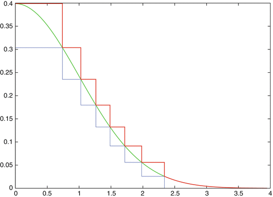
Ziggurat with N = 8 layers, for 0 ≤ x ≤ 4. The heavy-line zigzag (in red) on the right and above the graph of the normal density f (in green) is the major z with z(x) ≥ f(x), which represents the right-hand bound of the horizontal ziggurat boxes. For N = 8 the area of each ziggurat segment is 0.070283. The zigzag in blue that is below f bounds the area, in which the creation of a normally distributed sample essentially only costs one generation of \(U \sim \mathcal{U}[0,1]\)
- 10.
Check this by applying Theorem 2.11.
- 11.
The deterministic term “equidistributed” is not to be confused with the probabilistic “uniformly distributed”.
- 12.
As in Sect. 1.6.2.


References
Abramowitz, M., Stegun, I.: Handbook of Mathematical Functions. With Formulas, Graphs, and Mathematical Tables. Dover, New York (1968)
Achdou, Y., Pironneau, O.: Computational Methods for Option Pricing. SIAM, Philadelphia (2005)
Adams, R.A.: Sobolev Spaces. Academic Press, New York (1975)
AitSahlia, F., Carr, P.: American options: a comparison of numerical methods. In: Rogers, L.C.G., Talay, D. (eds.) Numerical Methods in Finance, pp. 67–87. Cambridge University Press, Cambridge (1997)
Alfonsi, A.: On the discretization schemes for the CIR (and Besselsquared) processes. Monte Carlo Methods Appl. 11, 355–384 (2005)
Almendral, A., Oosterlee, C.W.: Numerical valuation of options with jumps in the underlying. Appl. Numer. Math. 53, 1–18 (2005)
Almendral, A., Oosterlee, C.W.: Highly accurate evaluation of European and American options under the Variance Gamma process. J. Comput. Finance 10(1), 21–42 (2006)
Andersen, L., Andreasen, J.: Jump diffusion process: volatility smile fitting and numerical methods for option pricing. Rev. Deriv. Res. 4, 231–262 (2000)
Andersen, L., Broadie, M.: Primal-dual simulation algorithm for pricing multidimensional American options. Manag. Sci. 50, 1222–1234 (2004)
Andersen, L.B.G., Brotherton-Ratcliffe, R.: The equity option volatility smile: an implicit finite-difference approach. J. Comput. Finance 1(2), 5–38 (1997/1998)
Ané, T., Geman, H.: Order flow, transaction clock, and normality of asset returns. J. Finance 55, 2259–2284 (2000)
Arnold, L.: Stochastic Differential Equations (Theory and Applications). Wiley, New York (1974)
Arouna, B.: Robbins-Monro algorithms and variance reduction in finance. J. Comput. Finance 7(2), 35–61 (2003)
Artzner, P., Delbaen, F., Eber, J.-M., Heath, D.: Coherent measures of risk. Math. Finance 9, 203–228 (1999)
Avellaneda, M.: Quantitative Modeling of Derivative Securities. From Theory to Practice. Chapman & Hall, Boca Raton (2000)
Avellaneda, M., Levy, A., Parás, A.: Pricing and hedging derivative securities in markets with uncertain volatilities. Appl. Math. Finance 2, 73–88 (1995)
Avellaneda, M., Parás, A.: Dynamic hedging portfolios for derivative securities in the presence of large transaction costs. Appl. Math. Finance 1, 165–194 (1994)
Avellaneda, M., Parás, A.: Managing the volatility risk of derivative securities: the Lagrangian volatility model. Appl. Math. Finance 3, 21–53 (1996)
Babuška, I., Strouboulis, T.: The Finite Element Method and Its Reliability. Oxford Science, Oxford (2001)
Ball, C.A., Roma, A.: Stochastic volatility option pricing. J. Financ. Quant. Anal. 29, 589–607 (1994)
Barles, G.: Convergence of numerical schemes for degenerate parabolic equations arising in finance theory. In: Rogers, L.C.G., Talay, D. (eds.) Numerical Methods in Finance, pp. 2–21. Cambridge University Press, Cambridge (1997)
Barles, G., Burdeau, J., Romano, M., Samsœn, N.: Critical stock prices near expiration. Math. Finance 5, 77–95 (1995)
Barles, G., Daher, Ch., Romano, M.: Convergence of numerical schemes for parabolic equations arising in finance theory. Math. Models Methods Appl. Sci. 5, 125–143 (1995)
Barles, G., Soner, H.M.: Option pricing with transaction costs and a nonlinear Black-Scholes equation. Finance Stochast. 2, 369–397 (1998)
Barndorff-Nielsen, O.E.: Processes of normal inverse Gaussian type. Finance Stochast. 2, 41–68 (1997)
Barone-Adesi, G., Whaley, R.E.: Efficient analytic approximation of American option values. J. Finance 42, 301–320 (1987)
Barone-Adesi, G., Whaley, R.E.: On the valuation of American put options on dividend-paying stocks. Adv. Futures Options Res. 3, 1–13 (1988)
Barraquand, J., Pudet, T.: Pricing of American path-dependent contingent claims. Math. Finance 6, 17–51 (1996)
Barrett, R., et al.: Templates for the Solution of Linear Systems: Building Blocks for Iterative Methods. SIAM, Philadelphia (1994)
Bates, D.: Jumps and stochastic volatility: the exchange rate processes implicit in Deutschmark options. Rev. Financ. Stud. 9, 69–107 (1996)
Baxter, M., Rennie, A.: Financial Calculus. An Introduction to Derivative Pricing. Cambridge University Press, Cambridge (1996)
Behrends, E.: Introduction to Markov Chains. Vieweg, Braunschweig (2000)
Bellman, R.: Dynamic Programming. Princeton University Press, Princeton (1957)
Ben Hamida, S., Cont, R.: Recovering volatility from option prices by evolutionary optimization. J. Comput. Finance 8(4), 43–76 (2005)
Bensoussan, A.: On the theory of option pricing. Acta Appl. Math. 2, 139–158 (1984)
Berridge, S.J., Schumacher, J.M.: Pricing high-dimensional American options using local consistency conditions. In: Appleby, J.A.D., et al. (eds.) Numerical Methods for Finance. Chapman & Hall, Boca Raton (2008)
Billingsley, P.: Probability and Measure. Wiley, New York (1979)
Bischi, G.I., Sushko, I. (eds.): Dynamic Modelling in Economics & Finance. Special Issue of Chaos, Solitons and Fractals 29(3) (2006)
Bischi, G.I., Valori, V.: Nonlinear effects in a discrete-time dynamic model of a stock market. Chaos Solitons Fractals 11, 2103–2121 (2000)
Björk, T.: Arbitrage Theory in Continuous Time. Oxford University Press, Oxford (1998)
Black, F., Scholes, M.: The pricing of options and corporate liabilities. J. Polit. Econ. 81, 637–659 (1973)
Blomeyer, E.C.: An analytic approximation for the American put price for options with dividends. J. Financ. Quant. Anal. 21, 229–233 (1986)
Bouchaud, J.-P., Potters, M.: Theory of Financial Risks. From Statistical Physics to Risk Management. Cambridge University Press, Cambridge (2000)
Bouleau, N.: Martingales et Marchés Financiers. Edition Odile Jacob, Paris (1998)
Box, G.E.P., Muller, M.E.: A note on the generation of random normal deviates. Ann. Math. Stat. 29, 610–611 (1958)
Boyle, P.P.: Options: a Monte Carlo approach. J. Financ. Econ. 4, 323–338 (1977)
Boyle, P., Broadie, M., Glasserman, P.: Monte Carlo methods for security pricing. J. Econ. Dyn. Control 21, 1267–1321 (1997)
Boyle, P.P., Evnine, J., Gibbs, S.: Numerical evaluation of multivariate contingent claims. Rev. Financ. Stud. 2, 241–250 (1989)
Brachet, M.-E., Taflin, E., Tcheou, J.M.: Scaling transformation and probability distributions for time series. Chaos Solitons Fractals 11, 2343–2348 (2000)
Brandimarte, P.: Numerical Methods in Finance and Economics. A MATLAB-Based Introduction. Wiley, Hoboken (2006)
Breen, R.: The accelerated binomial option pricing model. J. Financ. Quant. Anal. 26, 153–164 (1991)
Brennan, M.J., Schwartz, E.S.: The valuation of American put options. J. Finance 32, 449–462 (1977)
Brenner, S.C., Scott, L.R.: The Mathematical Theory of Finite Element Methods, 2nd edn. Springer, New York (2002)
Brent, R.P.: On the periods of generalized Fibonacci recurrences. Math. Comput. 63, 389–401 (1994)
Briani, M., La Chioma, C., Natalini, R.: Convergence of numerical schemes for viscosity solutions to integro-differential degenerate parabolic problems arising in financial theory. Numer. Math. 98, 607–646 (2004)
Broadie, M., Detemple, J.: American option valuation: new bounds, approximations, and a comparison of existing methods. Rev. Financ. Stud. 9, 1211–1250 (1996)
Broadie, M., Detemple, J.: Recent advances in numerical methods for pricing derivative securities. In: Rogers, L.C.G., Talay, D. (eds.) Numerical Methods in Finance, pp. 43–66. Cambridge University Press, Cambridge (1997)
Broadie, M., Glasserman, P.: Pricing American-style securities using simulation. J. Econ. Dyn. Control 21, 1323–1352 (1997)
Broadie, M., Glasserman, P.: A stochastic mesh method for pricing high-dimensional American options. J. Comput. Finance 7(4), 35–72 (2004)
Brock, W.A., Hommes, C.H.: Heterogeneous beliefs and routes to chaos in a simple asset pricing model. J. Econ. Dyn. Control 22, 1235–1274 (1998)
Broyden, C.G.: The convergence of a class of double-rank minimization algorithms 1. General considerations. IMA J. Appl. Math. 6, 76–90 (1970)
Bruti-Liberati, N., Platen, E.: On weak predictor-corrector schemes for jump-diffusion processes in finance. Research Paper, University of Sydney (2006)
Bunch, D.S., Johnson, H.: A simple and numerically efficient valuation method for American puts using a modified Geske-Johnson approach. J. Finance 47, 809–816 (1992)
Caflisch, R.E., Morokoff, W., Owen, A.: Valuation of mortgaged-backed securities using Brownian bridges to reduce effective dimension. J. Comput. Finance 1(1), 27–46 (1997)
Carmona, R., Durrleman, V.: Generalizing the Black–Scholes formula to multivariate contingent claims. J. Comput. Finance 9(2), 43–67 (2005)
Carr, P., Faguet, D.: Fast accurate valuation of American options. Working paper, Cornell University (1995)
Carr, P., Geman, H., Madan, D.B., Yor, M.: Stochastic volatility for Lévy processes. Math. Finance 13, 345–382 (2003)
Carr, P., Madan, D.B.: Option valuation using the fast Fourier transform. J. Comput. Finance 2(4), 61–73 (1999)
Carr, P., Wu, L.: Time-changed Lévy processes and option pricing. J. Financ. Econ. 71, 113–141 (2004)
Carriere, J.F.: Valuation of the early-exercise price for options using simulations and nonparametric regression. Insur. Math. Econ. 19, 19–30 (1996)
Cash, J.R.: Two new finite difference schemes for parabolic equations. SIAM J. Numer. Anal. 21, 433–446 (1984)
Chan, T.F., Golub, G.H., LeVeque, R.J.: Algorithms for computing the sample variance: analysis and recommendations. Am. Stat. 37, 242–247 (1983)
Chen, S.-H. (ed.): Genetic Algorithms and Genetic Programming in Computational Finance. Kluwer, Boston (2002)
Chen, X., Chadam, J.: Analytical and numerical approximations for the early exercise boundary for American put options. Dyn. Continuous Discrete Impulsive Syst. A 10, 649–660 (2003)
Chen, X., Chadam, J.: A mathematical analysis of the optimal exercise boundary for American put options. SIAM J. Math. Anal. 38, 1613–1641 (2007)
Chiarella, C., Dieci, R., Gardini, L.: Speculative behaviour and complex asset price dynamics. In: Bischi, G.I. (ed.) Proceedings Urbino 2000 (2000)
Choi, H.I., Heath, D., Ku, H.: Valuation and hedging of options with general payoff under transaction costs. J. Kor. Math. Soc. 41, 513–533 (2004)
Chung, K.L., Williams, R.J.: Introduction to Stochastic Integration. Birkhäuser, Boston (1983)
Ciarlet, P.G.: Basic error estimates for elliptic problems. In: Ciarlet, P.G., Lions, J.L. (eds.) Handbook of Numerical Analysis, Vol. II. Elsevier/North-Holland, Amsterdam (1991)
Ciarlet, P., Lions, J.L.: Finite Difference Methods (Part 1) Solution of Equations in \(\mathbb{R}^{n}\). North-Holland/Elsevier, Amsterdam (1990)
Clarke, N., Parrot, A.K.: Multigrid for American option pricing with stochastic volatility. Appl. Math. Finance 6, 177–179 (1999)
Clewlow, L., Strickland, C.: Implementing Derivative Models. Wiley, Chichester (1998)
Coleman, T.F., Li, Y., Verma, Y.: A Newton method for American option pricing. J. Comput. Finance 5(3), 51–78 (2002)
Cont, R., Tankov, P.: Financial Modelling with Jump Processes. Chapman & Hall, Boca Raton (2004)
Cont, R., Voltchkova, E.: Finite difference methods for option pricing in jump-diffusion and exponential Lévy models. SIAM J. Numer. Anal. 43, 1596–1626 (2005)
Cox, J.C., Ingersoll, J.E., Ross, S.A.: A theory of the term structure of interest rates. Econometrica 53, 385–407 (1985)
Cox, J.C., Ross, S., Rubinstein, M.: Option pricing: a simplified approach. J. Financ. Econ. 7, 229–263 (1979)
Cox, J.C., Rubinstein, M.: Options Markets. Prentice Hall, Englewood Cliffs (1985)
Crandall, M., Ishii, H., Lions, P.L.: User’s guide to viscosity solutions of second order partial differential equations. Bull. Am. Math. Soc. 27, 1–67 (1992)
Crank, J.: Free and Moving Boundary Problems. Clarendon Press, Oxford (1984)
Crank, J.C., Nicolson, P.: A practical method for numerical evaluation of solutions of partial differential equations of the heat-conductive type. Proc. Camb. Philos. Soc. 43, 50–67 (1947)
Cryer, C.: The solution of a quadratic programming problem using systematic overrelaxation. SIAM J. Control 9, 385–392 (1971)
Cyganowski, S., Kloeden, P., Ombach, J.: From Elementary Probability to Stochastic Differential Equations with MAPLE. Springer, Heidelberg (2001)
Dahlbokum, A.: Empirical performance of option pricing models based on time-changed Lévy processes. Available at SSRN: http://ssrn.com/abstract=1675321 (2010)
Dai, M.: A closed-form solution for perpetual American floating strike lookback options. J. Comput. Finance 4(2), 63–68 (2000)
Dai, T.-S., Lyuu, Y.-D.: The bino-trinomial tree: a simple model for efficient and accurate option pricing. J. Deriv. 17, 7–24 (2010)
Dana, R.-A., Jeanblanc, M.: Financial Markets in Continuous Time. Springer, Berlin (2003)
Dempster, M.A.H., Hutton, J.P.: Pricing American stock options by linear programming. Math. Finance 9, 229–254 (1999)
Dempster, M.A.H., Hutton, J.P., Richards, D.G.: LP valuation of exotic American options exploiting structure. J. Comput. Finance 2(1), 61–84 (1998)
Derman, E., Kani, I.: Riding on a smile. Risk 7, 32–39 (1994)
Detemple, J.: American options: symmetry properties. In: Jouini, E., et al. (eds.) Option Pricing, Interest Rates and Risk Management. Cambridge University Press, Cambridge (2001)
Deutsch, H.-P.: Derivatives and Internal Models. Palgrave, Houndmills (2002)
Devroye, L.: Non-uniform Random Variate Generation. Springer, New York (1986)
d’Halluin, Y., Forsyth, P.A., Labahn, G.: A semi-Lagrangian approach for American Asian options under jump diffusion. SIAM J. Sci. Comput. 27, 315–345 (2005)
d’Halluin, Y., Forsyth, P.A., Vetzal, K.R.: Robust numerical methods for contingent claims under jump diffusion processes. IMA J. Numer. Anal. 25, 87–112 (2005)
Dieci, R., Bischi, G.-I., Gardini, L.: From bi-stability to chaotic oscillations in a macroeconomic model. Chaos Solitons Fractals 12, 805–822 (2001)
Doeblin, W.: Sur l’équation de Kolmogorov (1940)
Doob, J.L.: Stochastic Processes. Wiley, New York (1953)
Dowd, K.: Beyond Value at Risk: The New Science of Risk Management. Wiley, Chichester (1998)
Duffie, D.: Dynamic Asset Pricing Theory, 2nd edn. Princeton University Press, Princeton (1996)
Duffie, D., Pan, J., Singleton, K.: Transform analysis and asset pricing for affine jump-diffusions. Econometrica 68, 1343–1376 (2000)
Dupire, B.: Pricing with a smile. Risk 7, 18–20 (1994)
Eberlein, E., Frey, R., Kalkbrener, M., Overbeck, L.: Mathematics in financial risk management. Jahresber. DMV 109, 165–193 (2007)
Eberlein, E., Keller, U.: Hyperbolic distributions in finance. Bernoulli 1, 281–299 (1995)
Egloff, D.: Monte Carlo algorithms for optimal stopping and statistical learning. Ann. Appl. Probab. 15, 1396–1432 (2005)
Ehrhardt, M. (ed.): Nonlinear Models in Mathematical Finance. New Research Trends in Option Pricing. Nova Science, Hauppauge (2008)
Ekström, E., Lötstedt, P., Tysk, J.: Boundary values and finite difference methods for the single factor term structure equation. Appl. Math. Finance 16, 253–259 (2009)
El Karoui, N., Jeanblanc-Picqué, M., Shreve, S.E.: Robustness of the Black and Scholes formula. Math. Finance 8, 93–126 (1998)
Elliott, C.M., Ockendon, J.R.: Weak and Variational Methods for Moving Boundary Problems. Pitman, Boston (1982)
Elliott, R.J., Kopp, P.E.: Mathematics of Financial Markets. Springer, New York (1999)
Embrechts, P., Klüppelberg, C., Mikosch, T.: Modelling Extremal Events. Springer, Berlin (1997)
Ender, M.: Model risk in option pricing. www.risknet.de/risknet-elibrary/kategorien/market-risk (2008)
Epps, T.W.: Pricing Derivative Securities. World Scientific, Singapore (2000)
Faigle, U., Schrader, R.: On the Convergence of Stationary Distributions in Simulated Annealing Algorithms. Inf. Process. Lett. 27, 189–194 (1988)
Fang, F., Oosterlee, C.W.: A novel option pricing method based on Fourier-cosine series expansions. SIAM J. Sci. Comput. 31, 826–848 (2008)
Fang, F., Oosterlee, C.W.: Pricing early-exercise and discrete barrier options by fourier-cosine series expansions. Numer. Math. 114, 27–62 (2009)
Feller, W.: An Introduction to Probability Theory and Its Applications. Wiley, New York (1950)
Fengler, M.R.: Semiparametric Modeling of Implied Volatility. Springer, Berlin (2005)
Figlewski, S., Gao, B.: The adaptive mesh model: a new approach to efficient option pricing. J. Financ. Econ. 53, 313–351 (1999)
Fishman, G.S.: Monte Carlo. Concepts, Algorithms, and Applications. Springer, New York (1996)
Fisz, M.: Probability Theory and Mathematical Statistics. Wiley, New York (1963)
Föllmer, H., Schied, A.: Stochastic Finance: An Introduction to Discrete Time. de Gruyter, Berlin (2002)
Forsyth, P.A., Vetzal, K.R.: Quadratic convergence for valuing American options using a penalty method. SIAM J. Sci. Comput. 23, 2095–2122 (2002)
Forsyth, P.A., Vetzal, K.R.: Numerical methods for nonlinear PDEs in finance. In: Duan, J.-C., Härdle, W.K., Gentle, J.E. (eds.) Handbook of Computational Finance, pp. 503–528. Springer, Berlin (2012)
Forsyth, P.A., Vetzal, K.R., Zvan, R.: A finite element approach to the pricing of discrete lookbacks with stochastic volatility. Appl. Math. Finance 6, 87–106 (1999)
Forsyth, P.A., Vetzal, K.R., Zvan, R.: Convergence of numerical methods for valuing path-dependent options using interpolation. Rev. Deriv. Res. 5, 273–314 (2002)
Fournié, E., Lasry, J.-M., Lebuchoux, J., Lions, P.-L., Touzi, N.: An application of Malliavin calculus to Monte Carlo methods in finance. Finance Stochast. 3, 391–412 (1999)
Franke, J., Härdle, W., Hafner, C.M.: Statistics of Financial Markets. Springer, Berlin (2004)
Freedman, D.: Brownian Motion and Diffusion. Holden Day, San Francisco (1971)
Frey, R., Patie, P.: Risk management for derivatives in illiquid markets: a simulation-study. In: Sandmann, K., Schönbucher, P. (eds.) Advances in Finance and Stochastics. Springer, Berlin (2002)
Frey, R., Stremme, A.: Market volatility and feedback effects from dynamic hedging. Math. Finance 7, 351–374 (1997)
Frutos, J. de: A spectral method for bonds. Comput. Oper. Res. 35, 64–75 (2008)
Fu, M.C., et al.: Pricing American options: a comparison of Monte Carlo simulation approaches. J. Comput. Finance 4(3), 39–88 (2001)
Fusai, G., Sanfelici, S., Tagliani, A.: Practical problems in the numerical solution of PDEs in finance. Rend. Studi Econ. Quant. 2001, 105–132 (2002)
Gander, M.J., Wanner, G.: From Euler, Ritz, and Galerkin to modern computing. SIAM Rev. 54, 627–666 (2012)
Geman, H., et al., eds.: Mathematical Finance. Bachelier Congress 2000. Springer, Berlin (2002)
Gentle, J.E.: Random Number Generation and Monte Carlo Methods. Springer, New York (1998)
Gerstner, T., Griebel, M.: Numerical integration using sparse grids. Numer. Algorithms 18, 209–232 (1998)
Gerstner, T., Griebel, M.: Dimension-adaptive tensor-product quadrature. Computing 71, 65–87 (2003)
Geske, R., Johnson, H.E.: The American put option valued analytically. J. Finance 39, 1511–1524 (1984)
Giles, M.: Variance reduction through multilevel Monte Carlo path calculations. In: Appleby, J.A.D., et al. (eds.) Numerical Methods for Finance. Chapman & Hall, Boca Raton (2008)
Giles, M., Glasserman, P.: Smoking adjoints: fast Monte Carlo methods. Risk 19, 88–92 (2006)
Gilks, W.R., Richardson, S., Spiegelhalter, D.J. (eds.): Markov Chain Monte Carlo in Practice. Chapman & Hall, Boca Raton (1996)
Glaser, J., Heider, P.: Arbitrage-free approximation of call price surfaces and input data risk. Quant. Finance 12, 61–73 (2012). doi:10.1080/14697688.2010.514005
Glasserman, P.: Monte Carlo Methods in Financial Engineering. Springer, New York (2004)
Glover, K.J., Duck, P.W., Newton, D.P.: On nonlinear models of markets with finite liquidity: some cautionary notes. SIAM J. Appl. Math. 70, 3252–3271 (2010)
Golub, G.H., Van Loan, C.F.: Matrix Computations, 3rd edn. The John Hopkins University Press, Baltimore (1996)
Goodman, J., Ostrov, D.N.: On the early exercise boundary of the American put option. SIAM J. Appl. Math. 62, 1823–1835 (2002)
Grandits, P.: Frequent hedging under transaction costs and a nonlinear Fokker-Planck PDE. SIAM J. Appl. Math. 62, 541–562 (2001)
Grüne, L., Kloeden, P.E.: Pathwise approximation of random ODEs. BIT 41, 710–721 (2001)
Hackbusch, W.: Multi-Grid Methods and Applications. Springer, Berlin (1985)
Hackbusch, W.: Elliptic Differential Equations: Theory and Numerical Treatment. Springer Series in Computational Mathematics, vol. 18. Berlin, Springer (1992)
Haentjens, T., in ’t Hout, K.: ADI finite difference discretization of the Heston-Hull-White PDE. In: Simos, T.E., et al. (eds.) Numerical Analysis and Applied Mathematics. AIP Conference Proceedings, vol. 1281, pp. 1995–1999 (2010)
Häggström, O.: Finite Markov Chains and Algorithmic Applications. Cambridge University Press, Cambridge (2002)
Hairer, E., Nørsett, S.P., Wanner, G.: Solving Ordinary Differential Equations I. Nonstiff Problems. Springer, Berlin (1993)
Halton, J.H.: On the efficiency of certain quasi-random sequences of points in evaluating multi-dimensional integrals. Numer. Math. 2, 84–90 (1960)
Hammersley, J.M., Handscomb, D.C.: Monte Carlo Methods. Methuen, London (1964)
Hämmerlin, G., Hoffmann, K.-H.: Numerical Mathematics. Springer, Berlin (1991)
Han, H., Wu, X.: A fast numerical method for the Black–Scholes equation of American options. SIAM J. Numer. Anal. 41, 2081–2095 (2003)
Harrison, J.M., Pliska, S.R.: Martingales and stochastic integrals in the theory of continuous trading. Stoch. Process. Appl. 11, 215–260 (1981)
Hart, J.F.: Computer Approximations. Wiley, New York (1968)
Haug, E.G.: The Complete Guide to Option Pricing Formulas, 2nd edn. 2007. McGraw-Hill, New York (1998)
He, C., Kennedy, J.S., Coleman, T., Forsyth, P.A., Li, Y., Vetzal, K.: Calibration and hedging under jump diffusion. Rev. Deriv. Res. 9, 1–35 (2006)
Heider, P.: A condition number for the integral representation of American options. J. Comput. Finance 11(2), 95–103 (2007/08)
Heider, P.: A second-order Nyström-type discretization for the early-exercise curve of American put options. Int. J. Comput. Math. 86, 982–991 (2009)
Heider, P.: Numerical methods for non-linear Black–Scholes equations. Appl. Math. Finance 17, 59–81 (2010)
Heider, P., Schaeling, D.: Numerical methods for American options in nonlinear Black–Scholes models. Preprint, Universität Köln (2010)
Heston, S.L.: A closed-form solution for options with stochastic volatility with applications to bond and currency options. Rev. Financ. Stud. 6, 327–343 (1993)
Heston, S., Zhou, G.: On the rate of convergence of discrete-time contingent claims. Math. Finance 10, 53–75 (2000)
Higham, D.J.: An algorithmic introduction to numerical solution of stochastic differential equations. SIAM Rev. 43, 525–546 (2001)
Higham, D.J.: An Introduction to Financial Option Valuation. Cambridge University Press, Cambridge (2004)
Higham, D.J., Kloeden, P.E.: Numerical methods for nonlinear stochastic differential equations with jumps. Numer. Math. 101, 101–119 (2005)
Higham, N.J.: Accuracy and Stability of Numerical Algorithms. SIAM, Philadelphia (1996)
Higham, N.J.: Computing the nearest correlation matrix — a problem from finance. IMA J. Numer. Anal. 22, 329–343 (2002)
Hilber, N., Matache, A.-M., Schwab, C.: Sparse wavelet methods for option pricing under stochastic volatility. J. Comput. Finance 8(4), 1–42 (2005)
Hofmann, N., Platen, E., Schweizer, M.: Option pricing under incompleteness and stochastic volatility. Math. Finance 2, 153–187 (1992)
Hoggard, T., Whalley, A.E., Wilmott, P.: Hedging option portfolios in the presence of transaction costs. Adv. Futur. Options Res. 7, 21–35 (1994)
Holmes, A.D., Yang, H.: A front-fixing finite element method for the valuation of American options. SIAM J. Sci. Comput. 30, 2158–2180 (2008)
Honoré, P., Poulsen, R.: Option pricing with EXCEL. In: Nielsen, S. (ed.): Programming Languages and Systems in Computational Economics and Finance, pp. 369–402. Kluwer, Amsterdam (2002)
Huang, J.-Z., Subrahmanyam, M.G., Yu, G.G.: Pricing and hedging American options: a recursive integration method. Rev. Financ. Stud. 9, 227–300 (1996)
Hull, J.C.: Options, Futures, and Other Derivatives, 4th edn. Prentice Hall, Upper Saddle River (2000)
Hull, J., White, A.: The use of the control variate technique in option pricing. J. Financ. Quant. Anal. 23, 237–251 (1988)
Hunt, P.J., Kennedy, J.E.: Financial Derivatives in Theory and Practice. Wiley, Chichester (2000)
Ikonen, S., Toivanen, J.: Pricing American options using LU decomposition. Appl. Math. Sci. 1, 2529–2551 (2007)
Ikonen, S., Toivanen, J.: Operator splitting methods for pricing American options under stochastic volatility. Numer. Math. 113, 299–324 (2009)
Ingersoll, J.E.: Theory of Financial Decision Making. Rowmann and Littlefield, Savage (1987)
Int-Veen, R.: Avoiding numerical dispersion in option valuation. Report Universität Köln 2002; Comput. Vis. Sci. 10, 185–195 (2007)
Isaacson, E., Keller, H.B.: Analysis of Numerical Methods. Wiley, New York (1966)
Jacod, J., Protter, P.: Probability Essentials, 2nd edn. Springer, Berlin (2003)
Jäckel, P.: Monte Carlo Methods in Finance. Wiley, Chichester (2002)
Jaillet, P., Lamberton, D., Lapeyre, B.: Variational inequalities and the pricing of American options. Acta Appl. Math. 21, 263–289 (1990)
Jamshidian, F.: An analysis of American options. Rev. Futur. Mark. 11, 72–80 (1992)
Jiang, L., Dai, M.: Convergence of binomial tree method for European/American path-dependent options. SIAM J. Numer. Anal. 42, 1094–1109 (2004)
Johnson, H.E.: An analytic approximation for the American put price. J. Financ. Quant. Anal. 18, 141–148 (1983)
Jonen, C.: An efficient implementation of a least-squares Monte Carlo method for valuing American-style options. Int. J. Comput. Math. 86, 1024–1039 (2009)
Jonen, C.: Efficient Pricing of High-Dimensional American-Style Derivatives: A Robust Regression Monte Carlo method. PhD dissertation, Universität Köln (2011). http://kups.ub.uni-koeln.de/4442
Joshi, M.S.: The Concepts and Practice of Mathematical Finance. Cambridge University Press, Cambridge (2003)
Ju, N.: Pricing an American option by approximating its early exercise boundary as a multipiece exponential function. Rev. Financ. Stud. 11, 627–646 (1998)
Kaebe, C., Maruhn, J.H., Sachs, E.W.: Adjoint-based Monte Carlo calibration of financial market models. Finance Stochast. 13, 351–379 (2009)
Kahaner, D., Moler, C., Nash, S.: Numerical Methods and Software. Prentice Hall Series in Computational Mathematics. Prentice Hall, Englewood Cliffs (1989)
Kallast, S., Kivinukk, A.: Pricing and hedging American options using approximations by Kim integral equations. Eur. Finance Rev. 7, 361–383 (2003)
Kallsen, J.: A didactic note on affine stochastic volatility models. In: Kabanov, Y., et al. (eds.) From Stochastic Calculus to Mathematical Finance. Springer, Berlin (2006)
Kamrad, B., Ritchken, P.: Multinomial approximating models for options with k state variables. Manag. Sci. 37, 1640–1652 (1991)
Kangro, R., Nicolaides, R.: Far field boundary conditions for Black-Scholes equations. SIAM J. Numer. Anal. 38, 1357–1368 (2000)
Kantorovich, L.W., Akilov, G.P.: Functional Analysis in Normed Spaces. Pergamon Press, Elmsford (1964)
Karatzas, I., Shreve, S.E.: Brownian Motion and Stochastic Calculus, 2nd edn. Springer Graduate Texts. Springer, New York (1991)
Karatzas, I., Shreve, S.E.: Methods of Mathematical Finance. Springer, New York (1998)
Kat, H.M.: Pricing Lookback options using binomial trees: an evaluation. J. Financ. Eng. 4, 375–397 (1995)
Kebaier, A.: Statistical Romberg extrapolation: a new variance reduction method and applications to option pricing. Ann. Appl. Probab. 15, 2681–2705 (2005)
Kemna, A.G.Z., Vorst, A.C.F.: A pricing method for options based on average asset values. J. Bank. Finance 14, 113–129 (1990)
Khaliq, A.Q.M., Voss, D.A., Yousuf, M.: Pricing exotic options with L-stable Padé schemes. J. Bank. Finance 31, 3438–3461 (2007)
Kim, J.: The analytic valuation of American options. Rev. Financ. Stud. 3, 547–572 (1990)
Kirkpatrick, S., Gelatt, C.D., Vecchi, M.P.: Optimization by simulated annealing. Science 220, 671–680 (1983)
Klassen, T.R.: Simple, fast and flexible pricing of Asian options. J. Comput. Finance 4(3), 89–124 (2001)
Kloeden, P.E., Platen, E.: Numerical Solution of Stochastic Differential Equations. Springer, Berlin (1992)
Knuth, D.: The Art of Computer Programming, vol. 2. Addison-Wesley, Reading (1995)
Kocis, L., Whiten, W.J.: Computational investigations of low-discrepancy sequences. ACM Trans. Math. Softw. 23, 266–294 (1997)
Korn, R., Müller, S.: The decoupling approach to binomial pricing of multi-asset options. J. Comput. Finance 12(3), 1–30 (2009)
Kou, S.G.: A jump diffusion model for option pricing. Manag. Sci. 48, 1086–1101 (2002)
Kovalov, P., Linetsky, V., Marcozzi, M.: Pricing multi-asset American options: a finite element method-of-lines with smooth penalty. J. Sci. Comput. 33, 209–237 (2007)
Kreiss, H.O., Thomée, V., Widlund, O.: Smoothing of initial data and rates of convergence for parabolic difference equations. Commun. Pure Appl. Math. 23, 241–259 (1970)
Kröner, D.: Numerical Schemes for Conservation Laws. Wiley, Chichester (1997)
Krylov, N.V.: Controlled Diffusion Processes. Springer, Heidelberg (1980)
Kwok, Y.K.: Mathematical Models of Financial Derivatives. Springer, Singapore (1998)
Kwok, Y.K., Leung, K.S., Wong, H.Y.: Efficient options pricing using the Fast Fourier Transform. In: Duan, J.-C., Härdle, W.K., Gentle, J.E. (eds.) Handbook of Computational Finance, pp. 579–604. Springer, Berlin (2012)
Lambert, J.D.: Numerical Methods for Ordinary Differential Systems. The Initial Value Problem. Wiley, Chichester (1991)
Lamberton, D., Lapeyre, B.: Introduction to Stochastic Calculus Applied to Finance. Chapman & Hall, London (1996)
Lange, K.: Numerical Analysis for Statisticians. Springer, New York (1999)
L’Ecuyer, P.: Tables of linear congruential generators of different sizes and good lattice structure. Math. Comput. 68, 249–260 (1999)
Leentvaar, C.C.W., Oosterlee, C.W.: On coordinate transformation and grid stretching for sparse grid pricing of basket options. J. Comput. Math. 222, 193–209 (2008)
Lehn, J.: Random number generators. GAMM-Mitteilungen 25, 35–45 (2002)
Leisen, D.P.J.: Pricing the American put option: a detailed convergence analyis for binomial models. J. Econ. Dyn. Control 22, 1419–1444 (1998)
Leisen, D.P.J.: The random-time binomial model. J. Econ. Dyn. Control 23, 1355–1386 (1999)
Leisen, D.P.J., Reimer, M.: Binomial models for option valuation – examining and improving convergence. Appl. Math. Finance 3, 319–346 (1996)
Leland, H.E.: Option pricing and replication with transaction costs. J. Finance 40, 1283–1301 (1985)
Levy, G.: Computational finance using C and C#. Elsevier, Amsterdam (2008)
Longstaff, F.A., Schwartz, E.S.: Valuing American options by simulation: a simple least-squares approach. Rev. Financ. Stud. 14, 113–147 (2001)
Lord, R., Fang, F., Bervoets, F., Oosterlee, C.W.: A fast and accurate FFT-based method for pricing early-exercise options under Lévy processes. SIAM J. Sci. Comput. 30, 1678–1705 (2008)
Lux, T.: The socio-economic dynamics of speculative markets: interacting agents, chaos, and the fat tails of return distributions. J. Econ. Behav. Organ. 33, 143–165 (1998)
Lyons, T.J.: Uncertain volatility and the risk-free synthesis of derivatives. Appl. Math. Finance 2, 117–133 (1995)
Lyuu, Y.-D.: Financial Engineering and Computation. Principles, Mathematics, Algorithms. Cambridge University Press, Cambridge (2002)
MacMillan, L.W.: Analytic approximation for the American put option. Adv. Futur. Opt. Res. 1, 119–139 (1986)
Madan, D.B., Seneta, E.: The variance-gamma (V.G.) model for share market returns. J. Bus. 63, 511–524 (1990)
Mainardi, R., Roberto, M., Gorenflo, R., Scalas, E.: Fractional calculus and continuous-time finance II: the waiting-time distribution. Physica A 287, 468–481 (2000)
Maller, R.A., Solomon, D.H., Szimayer, A.: A multinomial approximation for American option prices in Lévy process models. Math. Finance 16, 613–633 (2006)
Mandelbrot, B.B.: A multifractal walk down Wall Street. Sci. Am. 280, 70–73 (1999)
Manteuffel, T.A., White, A.B., Jr.: The numerical solution of second-order boundary value problems on nonuniform meshes. Math. Comput. 47, 511–535 (1986)
Marchesi, M., Cinotti, S., Focardi, S., Raberto, M.: Development and testing of an artificial stock market. In: Bischi, G.I. (ed.) Proceedings Urbino 2000 (2000)
Marsaglia, G.: Random numbers fall mainly in the planes. Proc. Natl. Acad. Sci. USA 61, 23–28 (1968)
Marsaglia, G., Bray, T.A.: A convenient method for generating normal variables. SIAM Rev. 6, 260–264 (1964)
Marsaglia, G., Tsang, W.W.: The ziggurat method for generating random variables. J. Stat. Softw. 5(8), 1–7 (2000)
Mascagni, M.: Parallel pseudorandom number generation. SIAM News 32, 5 (1999)
Matache, A.-M., von Petersdorff, T., Schwab, C.: Fast deterministic pricing of options on Lévy driven assets. Report 2002–11, Seminar for Applied Mathematics, ETH Zürich (2002)
Matsumoto, M., Nishimura, T.: Mersenne twister: a 623-dimensionally equidistributed uniform pseudorandom number generator. ACM Trans. Model. Comput. Simul. 8, 3–30 (1998)
Mayo, A.: Fourth order accurate implicit finite difference method for evaluating American options. In: Proceedings of Computational Finance, London (2000)
McCarthy, L.A., Webber, N.J.: Pricing in three-factor models using icosahedral lattices. J. Comput. Finance 5(2), 1–33 (2001/02)
McDonald, R.L., Schroder, M.D.: A parity result for American options. J. Comput. Finance 1(3), 5–13 (1998)
Mel’nikov, A.V., Volkov, S.N., Nechaev, M.L.: Mathematics of Financial Obligations. American Mathematical Society, Providence (2002)
Merton, R.C.: Theory of rational option pricing. Bell J. Econ. Manag. Sci. 4, 141–183 (1973)
Merton, R.: Option pricing when underlying stock returns are discontinous. J. Financ. Econ. 3, 125–144 (1976)
Merton, R.C.: Continuous-Time Finance. Blackwell, Cambridge (1990)
Metwally, S.A.K., Atiya, A.: Using Brownian bridge for fast simulation of jump-diffusion processes and barrier options. J. Derv. 10, 43–54 (2002)
Meyer, G.H.: Numerical Investigation of early exercise in American puts with discrete dividends. J. Comput. Finance 5(2), 37–53 (2002)
Mikosch, T.: Elementary Stochastic Calculus, with Finance in View. World Scientific, Singapore (1998)
Mil’shtein, G.N.: Approximate integration of stochastic differential equations. Theory Probab. Appl. 19, 557–562 (1974)
Milshtein, G.N.: A method of second-order accuracy integration of stochastic differential equations. Theory Probab. Appl. 23, 396–401 (1978)
van Moerbeke, P.: On optimal stopping and free boundary problems. Rocky Mt. J. Math. 4, 539–578 (1974)
Moro, B.: The full Monte. Risk 8, 57–58 (1995)
Morokoff, W.J.: Generating quasi-random paths for stochastic processes. SIAM Rev. 40, 765–788 (1998)
Morokoff, W.J., Caflisch, R.E.: Quasi-random sequences and their discrepancies. SIAM J. Sci. Comput. 15, 1251–1279 (1994)
Morton, K.W.: Numerical Solution of Convection-Diffusion Problems. Chapman & Hall, London (1996)
Musiela, M., Rutkowski, M.: Martingale Methods in Financial Modelling, 2nd edn. 2005. Springer, Berlin (1997)
Neftci, S.N.: An Introduction to the Mathematics of Financial Derivatives. Academic Press, San Diego (1996)
Newton, N.J.: Continuous-time Monte Carlo methods and variance reduction. In: Rogers, L.C.G., Talay, D. (eds.) Numerical Methods in Finance, pp. 22–42. Cambridge University Press, Cambridge (1997)
Niederreiter, H.: Quasi-Monte Carlo methods and pseudo-random numbers. Bull. Am. Math. Soc. 84, 957–1041 (1978)
Niederreiter, H.: Random Number Generation and Quasi-Monte Carlo Methods. Society for Industrial and Applied Mathematics, Philadelphia (1992)
Niederreiter, H., Jau-Shyong Shiue, P. (eds.): Monte Carlo and Quasi-Monte Carlo methods in scientific computing. In: Proceedings of a Conference at the University of Nevada, Las Vegas, Nevada, USA, 1994. Springer, New York (1995)
Nielsen, B.F., Skavhaug, O., Tveito, A.: Penalty and front-fixing methods for the numerical solution of American option problems. J. Comput. Finance 5(4), 69–97 (2002)
Nielsen, B.F., Skavhaug, O., Tveito, A.: Penalty methods for the numerical solution of American multi-asset option problems. J. Comput. Appl. Math. 222, 3–16 (2008)
Nielsen, L.T.: Pricing and Hedging of Derivative Securities. Oxford University Press, Oxford (1999)
Øksendal, B.: Stochastic Differential Equations. Springer, Berlin (1998)
Omberg, E.: The valuation of American put options with exponential exercise policies. Adv. Futur. Opt. Res. 2, 117–142 (1987)
Oosterlee, C.W.: On multigrid for linear complementarity problems with application to American-style options. Electron. Trans. Numer. Anal. 15, 165–185 (2003)
Panini, R., Srivastav, R.P.: Option pricing with Mellin transforms. Math. Comput. Model. 40, 43–56 (2004)
Papageorgiou, A., Traub, J.F.: New results on deterministic pricing of financial derivatives. Columbia University Report CUCS-028-96 (1996)
Paskov, S., Traub, J.: Faster valuation of financial derivatives. J. Portf. Manag. 22, 113–120 (1995)
Pelsser, A., Vorst, T.: The binomial model and the Greeks. J. Deriv. 1, 45–49 (1994)
Peyret, R., Taylor, T.D.: Computational Methods for Fluid Flow. Springer, New York (1983)
Pham, H.: Optimal stopping, free boundary, and American option in a jump-diffusion model. Appl. Math. Optim. 35, 145–164 (1997)
Pironneau, O., Hecht, F.: Mesh adaption for the Black & Scholes equations. East-West J. Numer. Math. 8, 25–35 (2000)
Platen, E.: An introduction to numerical methods for stochastic differential equations. Acta Numer. 8, 197–246 (1999)
Pliska, S.R.: Introduction to Mathematical Finance. Discrete Time Models. Blackwell, Malden (1997)
Pooley, D.M., Forsyth, P.A., Vetzal, K.R.: Numerical convergence properties of option pricing PDEs with uncertain volatility. IMA J. Numer. Anal. 23, 241–267 (2003)
Pooley, D.M., Forsyth, P.A., Vetzal, K., Simpson, R.B.: Unstructured meshing for two asset barrier options. Appl. Math. Finance 7, 33–60 (2000)
Pooley, D.M., Vetzal, K.R., Forsyth, P.A.: Convergence remedies for non-smooth payoffs in option pricing. J. Comput. Finance 6(4), 25–40 (2003)
Press, W.H., Teukolsky, S.A., Vetterling, W.T., Flannery, B.P.: Numerical Recipes in FORTRAN. The Art of Scientific Computing, 2nd edn. Cambridge University Press, Cambridge (1992)
Protter, P.E.: Stochastic Integration and Differential Equations. Springer, Berlin (2004)
Quarteroni, A., Sacco, R., Saleri, F.: Numerical Mathematics. Springer, New York (2000)
Quecke, S.: Efficient numerical methods for pricing American options under Lévy models. PhD-dissertation, Universität Köln (2007). http://kups.ub.uni-koeln.de/2018
Rannacher, R.: Finite element solution of diffusion problems with irregular data. Numer. Math. 43, 309–327 (1984)
Rebonato, R.: Interest-Rate Option Models: Understanding, Analysing and Using Models for Exotic Interest-Rate Options. Wiley, Chichester (1996)
Reisinger, C.: Numerische Methoden für hochdimensionale parabolische Gleichungen am Beispiel von Optionspreisaufgaben. PhD Thesis, Universität Heidelberg (2004)
Rendleman, R.J., Bartter, B.J.: Two-state option pricing. J. Finance 34, 1093–1110 (1979)
Revuz, D., Yor, M.: Continuous Martingales and Brownian Motion. Springer, Berlin (1991)
Ribeiro, C., Webber, N.: A Monte Carlo method for the normal inverse Gaussian option valuation model using an inverse Gaussian bridge. Working paper, City University, London (2002)
Ribeiro, C., Webber, N.: Valuing path dependent options in the variance-gamma model by Monte Carlo with a gamma bridge. J. Comput. Finance 7(2), 81–100 (2003/04)
Ripley, B.D.: Stochastic Simulation. Wiley Series in Probability and Mathematical Statistics. Wiley, New York (1987)
Risken, H.: The Fokker-Planck Equation. Springer, Berlin (1989)
Rogers, L.C.G.: Monte Carlo valuation of American options. Math. Finance 12, 271–286 (2002)
Rogers, L.C.G., Shi, Z.: The value of an Asian option. J. Appl. Probab. 32, 1077–1088 (1995)
Rogers, L.C.G., Talay, D. (eds.): Numerical Methods in Finance. Cambridge University Press, Cambridge (1997)
Rubinstein, M.: Implied binomial trees. J. Finance 69, 771–818 (1994)
Rubinstein, M.: Return to oz. Risk 7(11), 67–71 (1994)
Rubinstein, R.Y.: Simulation and the Monte Carlo Method. Wiley, New York (1981)
Ruppert, D.: Statistics and Finance. An Introduction. Springer, New York (2004)
Saad, Y.: Iterative Methods for Sparse Linear Systems, 2nd edn. SIAM, Philadelphia (2003)
Saito, Y., Mitsui, T.: Stability analysis of numerical schemes for stochastic differential equations. SIAM J. Numer. Anal. 33, 2254–2267 (1996)
Sato, K.-I.: Lévy Processes and Infinitely Divisible Distributions. Cambridge University Press, Cambridge (1999)
Schöbel, R., Zhu, J.: Stochastic volatility with an Ornstein-Uhlenbeck process: an extension. Eur. Finance Rev. 3(1), 23–46 (1999)
Schönbucher, P.J., Wilmott, P.: The feedback effect of hedging in illiquid markets. SIAM J. Applied Mathematics 61, 232–272 (2000)
Schoenmakers, J.G.M., Heemink, A.W.: Fast Valuation of Financial Derivatives. J. Comput. Finance 1, 47–62 (1997)
Schoutens, W.: Lévy Processes in Finance. Wiley, Chichester (2003)
Schuss, Z.: Theory and Applications of Stochastic Differential Equations. Wiley Series in Probability and Mathematical Statistics. Wiley, New York (1980)
Schwarz, H.R.: Numerical Analysis. Wiley, Chichester (1989)
Schwarz, H.R.: Methode der finiten Elemente. Teubner, Stuttgart (1991)
Seydel, R.: Practical Bifurcation and Stability Analysis, 3rd edn. Springer Interdisciplinary Applied Mathematics, vol. 5. Springer, New York (2010)
Seydel, R.U.: Lattice approach and implied trees. In: Duan, J.-C., Härdle, W.K., Gentle, J.E. (eds.) Handbook of Computational Finance, pp. 551–577. Springer, Berlin (2012)
Seydel, R.U.: Risk and computation. In: Glau, K., Scherer, M., Zagst, R. (eds.) Innovations in Quantitative Risk Management, pp. 305–316. Springer, Heidelberg (2015)
Shiryaev, A.N.: Essentials of Stochastic Finance. Facts, Models, Theory. World Scientific, Singapore (1999)
Shreve, S.E.: Stochastic Calculus for Finance II. Continuous-Time Models. Springer, New York (2004)
Smith, G.D.: Numerical Solution of Partial Differential Equations: Finite Difference Methods, 2nd edn. Clarendon Press, Oxford (1978)
Smithson, C.: Multifactor options. Risk 10(5), 43–45 (1997)
Spanier, J., Maize, E.H.: Quasi-random methods for estimating integrals using relatively small samples. SIAM Rev. 36, 18–44 (1994)
Stauffer, D.: Percolation models of financial market dynamics. Adv. Complex Syst. 4, 19–27 (2001)
Steele, J.M.: Stochastic Calculus and Financial Applications. Springer, New York (2001)
Steiner, M., Wallmeier, M., Hafner, R.: Baumverfahren zur Bewertung diskreter Knock-Out-Optionen. OR Spektrum 21, 147–181 (1999)
Stoer, J., Bulirsch, R.: Introduction to Numerical Analysis. Springer, Berlin (1996)
Stoer, J., Witzgall, C.: Convexity and Optimization in Finite Dimensions I. Springer, Berlin (1970)
Stojanovic, S.: Computational Financial Mathematics Using MATHEMATICA. Birkhäuser, Boston (2003)
Strang, G.: Computational Science and Engineering. Wellesley, Cambridge (2007)
Strang, G., Fix, G.: An Analysis of the Finite Element Method. Prentice-Hall, Englewood Cliffs (1973)
Sweby, P.K.: High resolution schemes using flux limiters for hyperbolic conservation laws. SIAM J. Numer. Anal. 21, 995–1011 (1984)
Tavella, D., Randall, C.: Pricing Financial Instruments. The Finite Difference Method. Wiley, New York (2000)
Tezuka, S.: Uniform Random Numbers: Theory and Practice. Kluwer, Dordrecht (1995)
Thomas, D.B., Luk, W., Leong, P.H.W., Villasenor, J.D.: Gaussian random number generators. ACM Comput. Surv. 39(4), Article 11 (2007)
Thomas, J.W.: Numerical Partial Differential Equations: Finite Difference Methods. Springer, New York (1995)
Thomas, J.W.: Numerical Partial Differential Equations. Conservation Laws and Elliptic Equations. Springer, New York (1999)
Tian, Y.: A modified lattice approach to option pricing. J. Futur. Mark. 13, 563–577 (1993)
Tian, Y.: A flexible binomial option pricing model. J. Futur. Mark. 19, 817–843 (1999)
Tilley, J.A.: Valuing American options in a path simulation model. Trans. Soc. Actuar. 45, 83–104 (1993)
Topper, J.: Finite element modeling of exotic options. In: OR Proceedings 1999, pp. 336–341 (2000)
Topper, J.: Financial Engineering with Finite Elements. Wiley, New York (2005)
Traub, J.F., Wozniakowski, H.: The Monte Carlo algorithm with a pseudo-random generator. Math. Comput. 58, 323–339 (1992)
Trottenberg, U., Oosterlee, C., Schüller, A.: Multigrid. Academic Press, San Diego (2001)
Tsay, R.S.: Analysis of Financial Time Series. Wiley, New York (2002)
van der Vorst, H.A.: Bi-CGSTAB: a fast and smoothly converging variant of Bi-CG for the solution of nonsymmetric linear systems. SIAM J. Sci. Stat. Comput. 13, 631–644 (1992)
Varga, R.S.: Matrix Iterative Analysis. Prentice Hall, Englewood Cliffs (1962)
Vellekoop, M.H., Nieuwenhuis, J.W.: Efficient pricing of derivatives on assets with discrete dividends. Appl. Math. Finance 13, 265–284 (2006)
Vichnevetsky, R.: Computer Methods for Partial Differential Equations. Volume I. Prentice-Hall, Englewood Cliffs (1981)
Villeneuve, S., Zanette, A.: Parabolic ADI methods for pricing American options on two stocks. Math. Oper. Res. 27, 121–149 (2002)
Vretblad, A.: Fourier Analysis and Its Applications. Springer, New York (2003)
Wallace, C.S.: Fast pseudorandom numbers for normal and exponential variates. ACM Trans. Math. Softw. 22(1), 119–127 (1996)
Wang, X., Phillips, P.C.B., Yu, J.: Bias in estimating multivariate and univariate diffusion. J. Econ. 161, 228–245 (2011)
Wesseling, P.: Principles of Computational Fluid Dynamics. Springer, Berlin (2001)
Wilmott, P.: Derivatives. Wiley, Chichester (1998)
Wilmott, P., Dewynne, J., Howison, S.: Option Pricing. Mathematical Models and Computation. Oxford Financial Press, Oxford (1996)
Wloka, J.: Partial Differential Equations. Cambridge University Press, Cambridge (1987)
Zagst, R.: Interest-Rate Management. Springer, Berlin (2002)
Zhang, J.E.: A semi-analytical method for pricing and hedging continuously sampled arithmetic average rate options. J. Comput. Finance 5(1), 59–79 (2001)
Zhao, Y., Ziemba, W.T.: Hedging errors with Leland’s option model in the presence of transaction costs. Finance Res. Lett. 4, 49–58 (2007)
Zhu, Y.-I., Wu, X., Chern, I.-L.: Derivative Securities and Difference Methods. Springer, New York (2004)
Zienkiewicz, O.C.: The Finite Element Method in Engineering Science. McGraw-Hill, London (1977)
Zvan, R., Forsyth, P.A., Vetzal, K.R.: Robust numerical methods for PDE models of Asian options. J. Comput. Finance 1(2), 39–78 (1997/98)
Zvan, R., Forsyth, P.A., Vetzal, K.R.: Penalty methods for American options with stochastic volatility. J. Comput. Appl. Math. 91, 199–218 (1998)
Zvan, R., Forsyth, P.A., Vetzal, K.R.: Discrete Asian barrier options. J. Comput. Finance 3(1), 41–67 (1999)
Zvan, R., Vetzal, K.R., Forsyth, P.A.: PDE methods for pricing barrier options. J. Econ. Dyn. Control 24, 1563–1590 (2000)
Author information
Authors and Affiliations
Rights and permissions
Copyright information
© 2017 Springer-Verlag London Ltd.
About this chapter
Cite this chapter
Seydel, R.U. (2017). Generating Random Numbers with Specified Distributions. In: Tools for Computational Finance. Universitext. Springer, London. https://doi.org/10.1007/978-1-4471-7338-0_2
Download citation
DOI: https://doi.org/10.1007/978-1-4471-7338-0_2
Published:
Publisher Name: Springer, London
Print ISBN: 978-1-4471-7337-3
Online ISBN: 978-1-4471-7338-0
eBook Packages: Mathematics and StatisticsMathematics and Statistics (R0)