Rapid Manufacturing

Abstract

This chapter defines rapid manufacturing (RM) as a technique for manufacturing solid objects by the sequential delivery of energy and/or material to specified points in space. Current practice is to control the manufacturing process by using a computer-generated mathematical model. This chapter compares the large speed and cost advantages of RM to alternative polymer or metal manufacturing techniques such as powder metallurgy manufacturing or die casting. Moreover, the RM as an application of solid freeform fabrication for direct manufacturing of goods is addressed. Unlike methods such as computer numerical control (CNC) milling, these techniques allow the fabricated parts to be of high geometric complexity.

These keywords were added by machine and not by the authors. This process is experimental and the keywords may be updated as the learning algorithm improves.

7.1 Rapid Manufacturing

Rapid manufacturing (RM), also known as direct manufacturing/direct fabrication/ digital manufacturing, has been defined in various ways. One widely accepted definition is “the use of an additive manufacturing process to construct parts that are used directly as finished products or components” [1]. If this process occurs in the R&D stage, it is called rapid prototyping (RP) [2]. In the USA, the term “Solid Freeform Fabrication” is preferred to rapid prototyping or RM [3]. According to Plesseria et al., starting with a 3-D CAD part model, this technique converts the model to a series of layers using software; these layers are transferred to the building machine in which they are “printed” from the material by different processes. After printing one layer, a new layer of material is deposited and so on. Postprocessing treatment may be supplemented [4]. In other words, RM is the fabrication of parts or components using additive manufacturing technologies. The part is shaped layer-by-layer and could be used as a functional product. In this technique, the removal cutting tools are not required to produce the physical products and the parts with complicated geometry may be fabricated [5]. RM is sometimes considered one of the RP applications. However, there is no clear distinction among definitions. RM's outputs are often usable products. Stereolithography (SLA), laser sintering (LS), and fused deposition modeling (FDM) are some of the typical RM machines. As shown in Fig. 7.1, RM can also be expressed as a branch of additive fabrication, which refers to the technologies employed to create physical models, prototypes, tools, or finished parts using 3-D scanning systems.

Fig. 7.1

Manufacturing processes tree and rapid manufacturing (RM) position [6]

7.1.1 Applications of Rapid Manufacturing

RM is widely used for both large- and small-scale products and components for a variety of applications in many different fields. The main applications of the RM can be categorized as follows [7].

7.1.1.1 Tooling and Industrial Applications

Fabrication of metal casting and injection mold has been one of the main applications of RM in recent years, and has been addressed in the literature [8–11].

7.1.1.2 Aerospace

RM products have found efficient applications in spacecraft structures (mirrors, structural panels, optical benches, etc.). They are made up of different titanium and aluminum alloys (with granulated powder) and other materials such as silicon carbide, metal ceramic composites (SiC/Alu, ferrous materials with SiC), and carbon fiber reinforced polymer (CFRP) [12].

7.1.1.3 Architecture and Construction

In today's construction, CAD/CAM technology, industrial robots, and machines which use direct numerical control and RM open up the architectural possibilities. The Buswell's research into the use of mega-scale RM for construction [13], Pegna's investigation of solid freeform construction [14], and Khoshnevis's development of a new layer-by-layer fabrication technique called contour crafting [15] are some of the attempts to apply RM in architecture and construction industry.

7.1.1.4 Military

The production costs of military complex airframe structures were notably reduced where direct metal deposition, an RM technique, was applied to build limited number of metallic parts [16].

7.1.1.5 Medical Applications

Medical application of RM is mainly due to its capability to build uniquely shaped products having complex geometry. Medical products like implants, dentures, and skull and facial bones are the components that often vary from one person to another. Some examples are (1) custom-made orthodontic appliances production using proprietary thermoplastic ink jetting technology and (2) ear prostheses and burn masks for patients by using thermo-jet printing and FDM [17, 18]. Other applications have been reported to manufacture patient-specific models (lead masks) as well as protective shields in cancer treatment by using 3-D photography and metal spraying technology [19]. Forming a prosthetic glove of nontoxic materials to cover a patient's damaged hand is another medical application [20, 21].

7.1.1.6 Electronics and Photonics

A new RM methodology based on a direct-write technique using a scanning laser system to pattern a single layered SU-8 for fabrication of embedded microchannels has been reported by Yu et al. [22]. Nijmeijer et al. explain how microlaminates, which are widely used in ceramic capacitors of electronic devices, are being made by an RM process: centrifugal injection casting (CIC) [23].

7.1.2 Rapid Manufacturing's Advantages and Disadvantages

RM conducted in parallel batch production has a large advantage in speed, cost, and quality over alternative manufacturing techniques such as laser ablation or die casting. RM changes the cost models in conventional supply chains and has a key role in producing and supplying cost-effective customized products [24]. Consequently, RM's popularity is growing on a daily basis. According to a Wohlers Associates survey, RM's applications in additive processes grew from 3.9 % in 2003 to 6.6 % in 2004 and 8.2 % in 2005 [25].

7.1.2.1 Advantages

RM's advantages can be studied from several design-related perspectives.

• Design complexity: One major benefit of the additive manufacturing processes is that it is possible to make parts of virtually any geometrical complexity at no extra cost while in every conventional manufacturing technique there is a direct link between the complexity of a design and its production cost. Therefore, for a given volume of component, it is possible to get the geometry (or complexity) for “free,” as the costs incurred for any given additive manufacturing technique are usually determined by the time needed to build a certain volume of part, which, in turn, is determined by the orientation that the component is built in [26].

• Design freedom: The advent of RM will have profound implications for the way in which designers work. Generally, designers have been taught to design objects that can be made easily with current technologies —this being mainly due to the geometry limitations of the available manufacturing processes. For molded parts, draft angles, constant wall thickness, location of split line, etc. have to be factored into the design. Because of the advancements in RM, geometry will no longer be a limiting factor in design [26].

• New design paradigm: RM has simplified the interaction between mechanical and aesthetic issues. With current RM capabilities, industrial designers can design and fabricate the parts without the need to consider issues such as draft angle and constant wall thickness that are needed for processes such as injection molding. Similarly, mechanical designers are able to manufacture any complexity of product they require with minimum education in the aesthetic design field [26].

7.1.2.2 Disadvantages

Like any other immature technology, RM has drawbacks and limitations which preclude its widespread commercial application. Some main disadvantages are as follows:

• Material cost: Today, the cost of most materials for additive systems is about 100–200 times greater than that of those used for injection molding [27].

• Material properties: Thermoplastics from LS have performed the best for RM applications. However, a limited choice of materials is available. Actually, materials for additive processes have not been fully characterized. Also, the properties (e.g., tensile property, tensile strength, yield strength, and fatigue) of the parts produced by the RP processes are not currently competitive with those of the parts produced by conventional manufacturing processes. Ogando reports that the properties of a part produced by the FDM process with acrylonitrile butadiene styrene (ABS) material are about 70–80 % of a molded part. In contrast, in some cases, results are more promising for the RP processes. For example, the properties of the metallic parts produced by the direct metal laser sintering (DMLS) process are “very similar to wrought properties and better than casting in many cases.” Also, in terms of surface quality, even the best RM processes need secondary machining and polishing to reach acceptable tolerance and surface finish [28].

• Support material removal: When production volumes are small, the removal of support material is usually not a big issue. When the volumes are much higher, it becomes an important consideration. Support material that is physically attached is of most concern.

• Process cost: At present, conventional manufacturing processes are much faster than additive processes such as RM. Based on a comparison study by the Loughborough University, the SLA of a plastic part for a lawn mower will become economical at the production rate of 5,500 parts. For FDM, the breakeven point is about 6,500 parts. Nevertheless, injection molding is found to be more economical when larger quantities must be produced [29].

7.2 Rapid Manufacturing Errors

One of the main challenges in RP and RM is deviation from the CAD part model. The accuracy will be obviously enhanced by increasing the number of layers (decreasing the layer thickness) but the manufactured part is never identical to its CAD file because of the essence of layer-by-layer fabrication. Three major RM errors are as follows.

7.2.1 Preprocess Error

While converting a CAD to standard tessellation language (STL) format (as machine input), the outer surface of the part is estimated to some triangles and this estimation causes this type of error, especially around the points with higher curvature (lower radius). Meshing with smaller triangles may diminish this error. However, it requires more time to process the file and a more complicated trajectory for laser (Fig. 7.2).

Fig. 7.2

More triangles result in more edges in each layer [30]

7.2.2 Process Error

As shown in Fig. 7.3, slicing the part causes a new type of error (chordal error) while building the part layer-by-layer. This error depends on the layer thickness and the average slope angel of the part [30].

Fig. 7.3

This error can be estimated as bc cos θ [30]

To minimize bc cos θ, the thickness of layer, bc, in the curved area should be decreased and it leads to lower step-stair effect and a more accurate product. Poor laser scanning mechanism may prompt another error during the process. The accuracy of laser beam emission and its angle with the part surface affect product quality so to make it smaller, the equipments and tools should be carefully inspected.

7.2.3 Postprocess Error

Two other types of errors that arise after the process are shrinkage and warpage errors. The product usually shrinks while cooling and this makes a deviation from its original design. Overestimation of CAD file at the design stage regarding the material properties and heating factors can reduce such an error. Warpage error is due to disparate distribution of heat in the part. Thermodynamic and binding force models are usually required to estimate and obviate this error [30].

7.3 Computer-Aided Rapid Manufacturing

Computer technology has served RM in many different aspects. In this section, tool path generation for RM by different CAD formats and computer-aided process selection are explained. The majority of the RP and RM processes use STL CAD format to extract the geometrical data of the model. The tool path generation from the STL file is explained in detail. Drawing exchange format (DXF) CAD file format is very complex and is mainly used either for data exchange between CAD software or tool path generation for the computer numerical control (CNC) machining process. However, the tool path generation method that is explained in this section can be an alternative approach for RM processes. Information about the standard for the exchange of product model data (STEP), an increasingly popular CAD format, is provided in this section.

7.3.1 Path Generation by Use of Drawing Exchange Format File

• What is a DXF file: The DXF is a CAD data file format developed by Autodesk to transfer data between AutoCAD and other programs. Each of the eight sections of a DXF file contains certain information about the drawing: HEADER section (for general information about the drawing), CLASSES section (for application-defined classes whose instances appear in the other sections), TABLES section (for definitions of named items), BLOCKS section (for describing the entities comprising each block in the drawing), ENTITIES section (for the drawing entities, including any block references), OBJECTS section (for the data that apply to nongraphical objects, used by AutoLISP and ObjectARX applications), and THUMBNAILIMAGE section (for the preview image for the DXF file) [31].

• DXF for tool path generation: Because of the complexity of the DXF files, generating a tool path from these files for any automated machining or fabricating process is very difficult. In such a tool path generation mechanism, geometrical data need to be identified and extracted from many other data available in a DXF file that are not useful for a tool path. Data can be extracted from models that are designed as two-dimensional (2-D or wireframe) or two and half dimensional (2.5-D or surface) objects. Extracting data from DXF files containing 2.5-D objects is more complex than doing so from DXF files containing 2-D objects because for 2-D objects, the geometrical data are stored in the form of the object end points (e.g., start and end points of a line) while for 2.5-D objects, the geometrical data of a model (e.g., the surface of a sphere) are stored in the form of many small rectangles. In such case, for each rectangle x, y, and z coordination of all four corners are stored (Fig. 7.4).

  Fig. 7.4

  

  DXF file data storage format for a 2.5-D object

• DXF file generation: Figure 7.5 illustrates the general steps to create a DXF file in the AutoCAD environment. As shown in this figure, after drawing the boundary of the object in wireframe format, a surface is generated to cover the entire outer boundary of the object. Then, after separating each face from the object, the entire data are stored in a DXF file. AutoCAD provides users with the flexibility to set a desirable number of meshes of the surface modeling in both horizontal and vertical directions.

  Fig. 7.5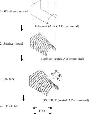

  

  DXF file generation procedure for a 2.5-D object in Auto-CAD environment

• Generating tool path from DXF files: In automated controlling of the tool in any machine that uses the tool path, regardless of the process or the machine type, geometrical data need to be extracted from the CAD file. Then, the tool path is calculated and generated on the basis of the geometry of the model as well as process and tool specification. A tool in here can be a milling machine tool, a laser cutter head, a welding machine gun head, or an extruder nozzle. Figure 7.6 shows the general steps of generating tool path from a DXF file [32].

  Fig. 7.6

  

  Tool path generation from DXF file

  As shown in Fig. 7.6, in addition to geometrical data, the desired quality of the final part affects the tool path output. Figure 7.7 illustrates two different tool path configurations for the same CAD data.

  Fig. 7.7

  

  Two different tool path configurations for the same CAD data

• Tool radius compensation: If the tool radius is considered for the tool path generation, which is a must for almost all path-based processes, then the complexity of the tool path generation process becomes more complicated. In the tool radius compensation, the tool path is calculated for the center of the tool (not for the touching point of the tool and the part). Therefore, in the tool path generation process, both the curvature of the object at the tool and object touching point and the tool specification (size and shape) are affecting the center of the tool coordination. The curvature of the object at any point is shown by the normal vector. A normal vector is a vector (often unit) that is perpendicular to a surface (Fig. 7.8).

  Fig. 7.8

  

  A surface and its normal vector

  Specifications of the tools may cover a variety of shapes and sizes. Three of the most common geometries of the tools are shown in Fig. 7.9. Most of the tools for machining and fabricating processes such as milling, extruding, welding, and laser beam are similar to one of these three geometries.

  Fig. 7.9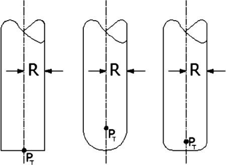

  

  Three common geometries for tools: 1 — flat end, 2 — ball end, and 3 — tip radius

• Flat end tool: To calculate the position of the tool center for the tool path, the geometrical data of four corners of each rectangular 3-D face is used. In this process, the unit normal vector of the 3-D face is calculated, Eqs. 7.1–7.3, and then it is used to determine the tool center position, Eqs. 7.4 – 7.6). In the flat end tools, the tool center is located at the same height (z level) as the tool and object touching point. This fact simplifies the calculation for the z level of the tool position. (Fig. 7.10).

  Fig. 7.10

  

  Flat end tool

  (7.1) (7.2) (7.3)

• Tool center: (7.4) (7.5) (7.6)

• Ball end tool: The calculation of tool center position for ball end tools is very similar to that for flat end tools. The only difference is the z level of the tool center that, similar to x and y coordination, needs to be determined by the unit normal vector of the 3-D faces (Fig. 7.11).

  Fig. 7.11

  

  Ball end tool

  (7.7) (7.8)

• Tool center: (7.9) (7.10) (7.11)

• Tip radius tool: The geometry of this type of tool is the combination of the last two tools (Fig. 7.12). The center part of this tool is a flat end tool while the edge of the tool has a fillet. Therefore, the position of the tool center is determined on the basis of the above two tools' calculations.

  Fig. 7.12

  

  Geometry of the tip radius tool

  (7.12)

• Tool center: (7.13) (7.14) (7.15)

Figure 7.13 illustrates a meshed CAD object (a) and the position of the object and tool path. At the end, it is necessary to mention that because of the complexity and limitations of the DXF files, it is very uncommon to use DXF to produce a tool path for RP, RM, or even 3-D and 2.5-D CNC machine code. Its application in CAM is usually limited to 2-D applications such as drilling.

Fig. 7.13

a A meshed CAD object and b the position of the object and tool path

7.3.2 Path Generation by Use of STL File

Every RM and RP system has its own specifications. The part boundary form, part filling method, and part separation from the surrounding material determine the tool path pattern for every layer. This tool path pattern could be a robotic movement in XY plane for FDM or contour crafting machines, a laser pattern for material solidification in SLA and selective laser sintering (SLS) machines, or a laser cutter pattern for a Laminated Object Manufacturing (LOM) machine. These processes require different tool path pattern generation strategies.

Therefore, unlike CNC standard tool path files (e.g. APT and G-Code), there is no standard tool path file for RP systems. Therefore, most of the new RM and RP require a new tool path generator or modification to the previous systems.

In this section, a tool path generation for the selective inhibition of sintering (SIS) process is presented. The software that is developed for this can be modified and adjusted for many other RP and RM processes. This system uses STL files with the ASCII format as input and works in two steps (Fig. 7.14).

Fig. 7.14

The two steps of slicing and tool path generation

7.3.2.1 Step 1 —Slicing Algorithm

In Step 1, the STL file is read as input. Slice files are then generated by executing the slicing algorithm. Only the intersection of those facets that intersect current Z = z is calculated and saved. In this step, one facet is read at a time from the STL file. Then the intersection lines of this facet with all XY planes for Z _min ≤ z ≤ Min{ Z _max, Max{ z _A, z _B, z _C}} are calculated. The intersection lines are stored in the specified file for the associated z increment. This results in one intersection line on each XY plane. By repeating this process for all facets, a set of slices is generated. This algorithm saves the data of only one facet in the computer memory; therefore only a small amount of computer memory is needed, and there is no practical limitation on the model size. In this step, each slice is saved in a separate file on the disk. This guarantees that Step 2 is run much faster than when all slices are saved in a single file. The example shown in Fig. 7.15 illustrates the slicing algorithm and Fig. 7.16 shows the flowchart of the slicing algorithm.

Fig. 7.15

Slicing algorithm steps

Fig. 7.16

The slicing algorithm

7.3.2.2 Step 2 —Tool Path Generation

After the completion of the slicing process, a set of vectors becomes available in each z increment. These vectors are not connected and are not in sequence. In the tool path generation process, the software starts from one vector and tries to find the next connected vector to this vector. Then it does the same for the newly found vector until it reaches the start point of the first vector (in the closed loop cases) or finds a vector with no leading attachment (in faulty STL files containing disconnections). To sort the vectors, the algorithm reads one vector at a time from a slice file and writes it to another file. This file is either a path file, when one vector is connected to the previous vector, or a temp file, when the vector is not connected to the previous vector. Therefore, the sorting process does not need a large amount of memory to sort the data, and there is no limitation on the number of vectors in a slice and on input file size. In addition, unlike many other slicing algorithms that cannot handle disconnections caused by faulty facets [33], this algorithm can generate a tool path even with disconnection errors in the STL file. At disconnection instances the system sends a message to a log file and turns the printer off and starts from a new vector. In either case, the printer is turned off and the system starts printing from another start point. Also for each selected vector, the possibility of hatch intersection points is investigated.

At the end of the path generation process for one slice, the hatch intersection points are sorted and written into a tool path file. After the arrangement of all vectors in one slice (z increment), the process starts arranging the vectors of the next slice. This process continues until all vectors in all slices are sorted. The diagram in Fig. 7.17 and the flowchart in Fig. 7.18 represent the tool path generation algorithm.

Fig. 7.17

Tool path generation steps

Fig. 7.18

The tool path generation algorithm

7.3.2.3 Implementation

Slicing and tool path generation algorithms have been implemented in the C programming language. The software has been successfully tested for several medium and large STL files up to 200 MB on different PCs and laptops. Figures 7.19 and 7.20 show the algorithm implementation as presented by the path simulation module of the system [34, 35].

Fig. 7.19

Visualization of models (up) and slices (bottom)

Fig. 7.20

Visualization of CAD file and the tool path in the Auto-CAD environment

7.3.3 Path Generation by Use of STEP File

STEP, introduced by PDES, Inc., is a neural format for exchanging product data among all the people or organizations who contribute to marketing, design, manufacturing, and other activities in the product life cycle. STEP (identified as ISO 10303) makes an independent platform to access, share, and manipulate the product information of its life cycle.

There are other types of product data exchange (PDE) models like IGES, DXF, DWG, VHDL, and STL which are used by many industries all over the world but STEP is known as a superior standard and is becoming highly popular over the other formats such as IGES [36].

7.3.3.1 Application Protocols

STEP is developed by a specific language of EXPRESS and includes a number of manageable and functional sections referred to as application protocol (AP). Each AP is in charge of an application of STEP. For example, AP224 or ISO 10303–224 are mechanical product definitions for process planning using machining features; AP203 is configuration-controlled 3-D designs of mechanical parts and assemblies. For the time being, only 22 APs have been approved as International Standards; however, it is expected that there will be hundreds of APs in the future.

Fig. 7.21

B-rep model of a simple cube: faces, edges, and vertices depicted in the model

STEP file contains all the required information for design, process planning, and other downstream activities; the implementation of STEP tools depends on the requirements and problem area in the organization. For process planning, a mechanical part based on its machining features, AP224, will be applicable as it classifies the features and can store and manage the data needed for each feature [37, 38].

7.3.3.2 Boundary Representation Model

Some APs contain boundary representation (B-rep) models for mechanical parts. For every 3-D part, B-rep expresses the surface boundary, which consists of the part's geometrical and topological information. Vertices, edges, and faces information is also represented by a B-rep model [39] (Fig. 7.21).

7.3.3.3 Using STEP for Tool Path Generation

No direct usage of STEP file to generate the tool path in RM has been reported. But as indicated, some of the application protocol contains B-rep information for the products. This information model can be extracted and used for tool path generation. Consider a part meshed with triangles and sliced in STL file format is replaced with a part having information of all the edges, faces, and vertices. Laser trajectory will be obtained by introducing the points of outer surfaces. This may not be applicable only for free-form parts with complex geometry as their B-rep information is not complete on the surfaces (Fig. 7.22).

Fig. 7.22

Boundary representation (B-rep) of a simple part [40]

Even with a B-rep model, slicing is required to determine the exact intersection points and feed the control system of laser scanning. A sample CAD model and its STEP file are shown in Figs. 7.23 and 7.24, respectively.

Fig. 7.23

A typical part to be rapid-manufactured

Fig. 7.24

A piece of a STEP file

AP240, numerical control process plans for machined parts (ISO 10303– 240:2005), is a part of ISO 10303 that specifies information requirements for the exchange, archival, and sharing of computer-interpretable numerical control (NC) process plan information and associated product definition data but it does not include specific machine tool controller codes. AP204, AP207, AP210, AP214, AP224, AP227, and AP240 are the applications which have boundary information of the corresponding parts and may be used for tool path generation. [41]

7.3.4 Rapid Manufacturing Process Selection and Simulation

Because of the inherent strengths and weaknesses of all RM processes, choosing the method best fitted to economical and technical objectives is a serious problem. This process selection is a multi-criteria decision making. Along with satisfying customer requirements, the functional product is expected to be manufactured to an adequate quality and at most reasonable cost in the shortest possible time. Other criteria such as product recyclability or serviceability may be considered.

One of the approaches for making such simulation in RP and RM uses computer software in order to create a virtual prototype. It is due to high material cost and prototyping of the real prototypes. Simulators help engineers to evaluate the performance of the process and minimize the number of repetitions to reach an appropriate prototype [42]. One successful attempt to introduce such simulators was made by Choi and Samavedam [43]. They developed a simulation software program to show the RM process layer-by-layer with SLS process. It shows also the relation between process parameters and time and accuracy of the product. The main advantages of running simulation in RP and RM are listed below:

• The cost of materials especially for some processes such as SLS is notable.

• The process of making the product is usually time-consuming.

• The energy consumption and equipment depreciation are high.

• The quantitative parameters of the prototype will be easily extracted.

• The product information may be shared with other persons or research centers [44].

VIRAPS (Virtual Rapid Prototyping System) is a simulation software program developed by Visual Basic and simulates some of the most common processes of RP and RM, like FDM, SLS, SLA, and LOM. Here we describe how VIRAPS works and the outcomes.

There are many criteria to consider in choosing the right RM process. Since it is a multi-criteria decision, an analytic hierarchy process (AHP) methodology could be applied to rank the most appropriate process according to the customer's criteria. Using software, RM processes are compared to each other on the basis of some common characteristics such as average time, cost, and quality of the finished products. The priority of these criteria is also determined by customer and the highest ranked RM process and machine is selected accordingly [45].

As a case study, SLS is considered for simulation. Suppose that a conic-shaped product is manufactured by SLS. The important inputs for this process are as follows:

• Part information (maximum dimensions, average slope, and layer thickness)

• Laser specification (laser type, laser power, beam diameter, and scan speed)

• Powder selection (here is steel-bronze)

• Setup time for each layer (the time required between creating each layer for setup)

• Cost parameters (direct cost, operation cost, and material cost)

The software also indicates the maximum and minimum allowed for some parameters such as scan speed or beam diameter and product weight according to the machine capabilities. Moreover, some parameters, such as type of laser, are automatically selected by the software [46] (Figs. 7.25 and 7.26).

Fig. 7.25

The SLS analytical simulation interface

Fig. 7.26

Software interface for process cost items

The outputs are shown in Fig. 7.27. This product will be made in 6.5 h and with the accuracy ratio of 73 and efficiency of 47 %. The total estimated cost is $344 and the number of layers according to the best orientation of the part is 500. These results are calculated on the basis of input information. For instance, the time in SLS is formulated below [30]:Velocity(v) (7.16) where velocity (v) = velocity of laser (mm/s), P ₁ = power of laser emission (watt), R = reflection ratio of laser reflector mirror, p = material density (g/mm³), d _b = beam diameter (mm), l _m = layer thickness (mm), C _P = specific heat capacity (J/K), T _m = material melting point (K), and T _b = laser scanning time (s).

Fig. 7.27

Process simulation outcomes

On the one hand, the time required for building the whole part is the time taken for making all the layers and the time of setup for each layer. On the other hand, the time of scanning each layer, T, is L _d/L _v in which L _d is the laser scanning distance and L _v is the laser scanning speed (7.17)where build time (total) = total time for building layers, T _li = scanning time for layer i, T _s = setup time for each layer, and N ₁ = number of layers.

Setup time is separately obtained by the following relations: (7.18) xwhere T _wd = time required for moving the part bed downward (s) T _d = time required for pouring a layer of material (s), T _wr = time required for moving the part bed upward (s) and T _h = time required for preheating the material (s)

Therefore, assuming each layer has thickness of l and the distance scanning of laser for layer i is d _si for a part with height of h we have (7.19)

7.4 Rapid Manufacturing Prospects

Today, RM is widely used in some companies. However, because of the material and process limitations of the current RM processes because of the lack of familiarity with these machines, RM is not as popular as it should be. It is estimated that in the next 10–20 years, engineers will recognize the benefits of RM processes [28].

References

Dickens P., Research goals in rapid manufacturing. Metalworking Production 148:21–22, 2004.
Hopkinson N., Hague R., Dickens P., Rapid Manufacturing, (Abstract). Germany: Wiley-VCH., 2005.
Soar R.C., Gibb A.G.F., Thorpe A., Buswell R.A., Freeform construction: mega-scale rapid manufacturing for construction. Automation in Construction 16:224–231, 2007.
Rochus P., Plesseria J.Y., Van Elsen M., Kruth J.P., Carrus R., Dormal T., New applications of rapid prototyping and rapid manufacturing (RP/RM) technologies for space instrumentation 61:352–359, 2007.
Hague R., Mansour S., Saleh N., Material and design considerations for rapid manufacturing. International Journal of Production Research 42:4691–4708, 2004.
Wohlers Associates Inc., What is Additive Fabrication? 2006.
Science group in groupsrv.com,http://www.groupsrv.com/science/index.php.
Nan Z., Gang W., Application of rapid prototyping techniques to rapid manufacturing of mould. Hebei Journal of Industrial Science & Technology 21:38–40, 2004.
Shi Y.-S., Cheng W., Huang N.-Y., Huang S.-H., Rapid manufacturing technology for casting mould. Zhuzao (Foundry) 54:382–385, 2005.
Li Y.-M., Hao Y., Huang N.-Y., Fan Z.-T., Dong X.-P., Liu H.-J. Casting-the key enabling technology promoting rapid manufacturing of metallic parts or moulds, Research Center of Die and Mould Technology, State Key Laboratory of New Non-ferrous Metal Materials, Lanzhou University of Technology.
Zhao J.F., Yu C.Y., Wu X.L., Jishu J.K.U., Zhang J.H., A new technology for rapid manufacturing of 3D moulds. Mechanical Science and Technology 20:419–420, 2001.
Plesseria J.Y., Van Elsen M., Kruth J.P., Carrus R., Dormal T., Rochus P., New applications of rapid prototyping and rapid manufacturing (RP/RM) technologies for space instrumentation 61:352–359, 2007.
Buswell R.A., Gibb A.G.F., Mega-scale Rapid Manufacturing for construction. Automation in Construction 16:24–31, 2007.
Pegna J., Exploratory investigation of solid freeform construction. Automation in Construction 5:427–437, 1997.
Khoshnevis B., Automated construction by contour crafting —related robotics and information sciences, Automation in Construction (special issue): The Best of ISARC 13:5–19, 2004.
Calder N.J., Place for rapid manufacturing in military airframe production. Materials Technology 15:34–37, 2000.
Product innovations, Rapid manufacturing produces custom lingual orthodontic appliances. Modern Casting 96:76, 2006.
Watson J., Rowson J.E., Holland J., Harris R.A., Williams D.J., Application of Rapid Manufacturing Techniques in Support of Maxillofacial Treatment: Evidence of the Requirements of Clinical Applications. Journal of Engineering Manufacture 219:469–475, 2005.
De Beer D.J., Truscott M., Booysen G.J., Barnard L.J., Van Der Walt J.G., Rapid manufacturing of patient-specific shielding masks, using RP in parallel with metal spraying. Rapid Prototyping Journal 11:298–303, 2005.
Alves N.M.F., Bartolo P.J.S., Ferreira J.C., Rapid manufacturing of medical prostheses. International Journal of Manufacturing Technology and Management 6:567–583, 2004.
Sanghera B., Naique S., Papaharilaou Y., Amis A., Preliminary study of rapid prototype medical models. Rapid Prototyping Journal 7:275–284, 2001.
Yu H., Balogun O., Li B., Murray T.W., Zhang X., Rapid Manufacturing of Embedded Microchannels from a Single Layered SU-8, and Determining the Dependence of SU-8 Young's Modulus on Exposure Dose with a Laser Acoustic Technique In: Proceedings of the 18th IEEE International Conference on Micro Electro Mechanical Systems, MEMS 2005, Miami —Technical Digest 654–657, 2005.
Biesheuvel P.M., Nijmeijer A., Kerkwijk B., Verweij H., Rapid manufacturing of microlami-nates by centrifugal injection casting. Advanced Engineering Materials 2:507–510, 2000.
Tuck C., Hague R., The pivotal role of rapid manufacturing in the Production of Cost-Effective Customised Products. International Journal of Mass Customisation 1:360–373, 2006.
Wohlers T., “Viewpoint,”Time-Compression Technologies, 2006.
Hague R., Design Opportunities with Rapid Manufacturing, Rapid Manufacturing Research Group, Wolfson School of Mechanical and Manufacturing Engineering., Loughborough University, Loughborough, UK.
Ogando J., Rapid manufacturing's role in the factory of the future. Design News, 2007.
Tuck C., Hague R., Make or buy analysis for rapid manufacturing. Rapid Prototyping Journal 13:23–29, 2007.
Choi S.H., Samavedam S., Modeling and optimization of rapid prototyping, Computers in Industry 47:39–53, 2002.
Revisions to the DXF Reference,http://www.autodesk.com/
Asiabanpour B., CAMAIRIC: A Computer Software in Computer Aided Manufacturing In: The 6th Annual Industrial Engineering Conference. Tehran, Iran., 1999.
Leong K.F., Chan C.K., Ng Y.M., A study of stereolithography file errors and repair. The International Journal of Advanced Manufacturing Technology 407–414 , 2004.
Asiabanpour B., Khoshnevis B., Machine path generation for the SIS process. Journal of Robotics and Computer Integrated Manufacturing 20:167–264 .
Asiabanpour B., Khoshnevis B., Palmer K., Advancements in the selective inhibition of sintering process development. Virtual and Physical Prototyping Journal 1:43–52, 2006.
Mangesh P., Bhandarkar N.R., STEP-based feature extraction from STEP geometry for Agile Manufacturing, Computers in Industry, 41(1): 3–24, 2000.
SCRA, Step Application Handbook, ISO 10303 Version 3, 2006.
ISO 13030–224, Industrial Automation Systems and Integration; Product Data Representation and Exchange, Part 224. Application protocol: Mechanical Product definition for process plans using machining features, 2001.
Shapiro V., Donald L. Vossler, “What is a parametric family of solids?”, Proceedings of the third ACM symposium on solid modeling and application Salt Lake City, Utah, ACM, New York, USA, 43–54, 1995, ISBN: 0-897-91-672-7.
Sequin C.H., Foundations of the computer graphics,http://www.cs.berkeley.edu/̃sequin/ CS184/IMGS/Breps.GIF
Kramer T.R., Huang H., Messina E., Proctor F.M., Scott H., A feature-based inspection and machining system. Computer-Aided Design 33:653–669, 2001.
Nee A.Y.C., Fuh J.Y., Miyazawa T., On the Improvement of the stereolithography (SL) process. Journal of Materials Processing Technology 113:262–268, 2001.
Choi S.H., Samavedam S., Modeling and optimization of rapid prototyping. Computers in Industry 47:39–53, 2002.
Choi S.H., Samavedam S., Visualization of rapid prototyping. Rapid Prototyping Journal 7:99–114, 2001.
Mokhtar A.R., Applying AHP Methodology to Select the Best Rapid Prototyping Technique In: The 32nd International Conference of Industrial Engineering, Ireland, Aug 2003.
Houshmand M., Mokhtar A.R., Analytical simulation of rapid prototyping process in a virtual environment. Journal of Science and Technology 28:86–91, 2005.
Author information
Authors and Affiliations
Editor information
Editors and Affiliations
Rights and permissions
Copyright information
© 2008 Springer Science+Business Media, LLC
About this chapter
Cite this chapter
Asiabanpour, B., Mokhtar, A., Houshmand, M. (2008). Rapid Manufacturing. In: Kamrani, A.K., Nasr, E.S.A. (eds) Collaborative Engineering. Springer, Boston, MA. https://doi.org/10.1007/978-0-387-47321-5_7
Download citation
DOI: https://doi.org/10.1007/978-0-387-47321-5_7
Publisher Name: Springer, Boston, MA
Print ISBN: 978-0-387-47319-2
Online ISBN: 978-0-387-47321-5
eBook Packages: EngineeringEngineering (R0)