Moving Frames and Differential Invariants on Fully Affine Planar Curves

Abstract

In this paper, by the affine analogue of the fundamental theorem for Euclidean planar curves, we classify the affine curves with constant affine curvatures. Note that we use the fully affine group and not the equi-affine subgroup consisting of area-preserving affine transformations. (Caution: much of the literature omits the “equi-” in their treatment.) According to the equivariant method of moving frames, explicit formulas for the generating affine differential invariants and invariant differential operators are constructed. At the same time, by using the fact that the affine transformation group GA$(2,\mathbb {R})$ can factor as a product of two subgroup $B\cdot \mathrm{SE}(2,\mathbb {R})$ and the moving frame of the subgroup SE$(2,\mathbb {R})$, we build the moving frame of GA$(2,\mathbb {R})$ and obtain the relations among invariants of group GA$(2,\mathbb {R})$ and its subgroup SE$(2,\mathbb {R})$. Applying the affine curvature to recognize affine equivalent objects is considered in the last part of this paper.

1 Introduction

In Euclidean differential geometry, the Frenet–Serret frame is a moving frame defined on a curve which can be constructed purely from the velocity and acceleration of the curve. The torsion and curvature are obtained by differentiating the frame, which describe completely how the frame evolves in time along the curve [4]. Special affine curvature, also known as the equi-affine curvature, is a particular type of curvature that is defined on a plane curve and remains unchanged under a special affine transformation (an affine transformation that preserves area) [16]. Hu and Liu studied centro-affine invariant arc length and centro-affine curvature functions of a curve in affine space directly by the parameter transformations and the centro-affine transformations [7, 13]. Yang and Yu defined the notion of affine curvatures on a discrete planar curve and studied the applications in self-affine fractals [24]. By using the equivariant method of moving frames, Olver gave the complete systems of functionally independent differential invariants for curves under centro-affine transformations and equi-affine transformations [21, 22]. Applications of full affine invariance to image processing can be found, for instance, in [25]. In this paper, we introduce and study the fully affine invariant arc length and fully affine curvature functions on a planar curve.

The arrangement of this paper is as follows: In Sect. 2, we introduce moving frames and the definitions. The equivariant method of moving frames is applied to generate affine differential invariants and invariant differential operators. In Sect. 3, we use the traditional method to obtain the fully affine invariants and then study the arc length and affine curvature. A classification for the planar curves with the constant affine curvatures is also given. Section 4 expresses the differential invariants for the affine transformation group in terms of the differential invariants of its subgroup. Finally, in Sect. 5, we investigate some applications of the affine curvature invariants.

2 Preliminaries

2.1 The Equivariant Method of Moving Frames

Let us first recall the basic equivariant moving frame method introduced by Fels and Olver [5, 6]. For more details, see [5, 6, 14, 15, 19]. Assume G is an r-dimensional Lie group acting smoothly on an m-dimensional manifold M with a left action, such that

$$\begin{aligned} G\times M \rightarrow M,\ \ h\cdot (g\cdot z)=(hg)\cdot z. \end{aligned}$$

A right (resp. left) group-based moving frame is a smooth, G-equivariant map $\rho :M\rightarrow G$, with respect to the action on M and the inverse right (resp. left) action of G on itself, specifically,

$$\begin{aligned} \rho : M\rightarrow G, \ \ \rho (g\cdot z)=\rho (z)g^{-1}\qquad (\mathrm {resp.} \ \ \rho (g\cdot z)=g\rho (z)). \end{aligned}$$

In many cases, right moving frames can be easier to compute.

Given a Lie group G acting on a manifold M, a moving frame exists in a neighborhood of a point $z\in M$ if and only if G acts freely and regularly near z; that is, the existence of a moving frame on the open subset $U\subset M$ is guaranteed if:

• 1. the intersection of the orbits with U has the same dimension as that of the group G and further foliate U (the regularity of the foliation is necessary);

• 2. there exists a submanifold $\mathcal {K}\subset U$ that intersects the orbits of U transversally, and the intersection $\mathcal {O}\cap \mathcal {K}$ contains a single point, and this submanifold $\mathcal {K}$ is known as the cross section and has dimension equal to $\dim (M)-\dim (G)$;

• 3. given a point $z\in \mathcal {O}(z)\cap U$, where $\mathcal {O}(z)$ is the orbit through z, the group element $h = \rho (z)\in G$ which takes z to a point $h\cdot z\in \mathcal {O}(z)\cap \mathcal {K}$ on the cross section is unique.

Given local coordinates $Z=(z_1,\ldots ,z_m)$ on M, let $\omega (g,z)=g\cdot z$ be the formulae for the transformed coordinates under the group transformation. The right moving frame $g=\rho (z)$ associated with the coordinate cross section $K=\{z_1=c_1,\ldots ,z_r=c_r\}$ is found by solving the normalization equations

$$\begin{aligned} \omega _1(g,z)=c_1,\ldots ,\omega _r(g,z)=c_r, \end{aligned}$$

(2.1)

for the group parameters $(g_1,\ldots ,g_r)$ in terms of the coordinates $z=(z_1,\ldots ,z_m)$. The remaining coordinates are the non-constant invariants.

Theorem 2.1

If $g=\rho (z)$ is the moving frame solution to Eq. (2.1), then

$$\begin{aligned} I_1(z)=\omega (\rho (z)\cdot z),\ldots , I_{z-r}(z)=\omega _m(\rho (z)\cdot z), \end{aligned}$$

(2.2)

form a complete system of functionally independent invariants.

Definition 2.2

The invariantization of a scalar function $F:M\rightarrow \mathbb {R}$ with respect to a right moving frame is the invariant function $I=\iota (F)$ defined by $I(z)=F(\rho (z)\cdot z)$.

However, most interesting group actions (Euclidean, affine, projective, etc.) are not free, and freeness typically fails because the dimension of the underlying manifold is not large enough, i.e., $\dim (M)=m < r = \dim (G)$. There are two basic methods for converting a non-free (but effective) action into a free action. The first is to look at the product action of G on a sufficiently large Cartesian product $M^{\times (n+1)}$, leading to joint invariants [18], which are especially interesting in classical algebra and numerical analysis [20, 23]. The second is to prolong the group action to a jet space $\mathbf {J}^n$ of suitably high order, which is the natural setting for the traditional moving frame theory, and leads to the classical differential invariants for the group [22]. Combining the two methods of prolongation and product will lead to joint differential invariants [18].

Definition 2.3

Given a smooth manifold M of dimension m and an integer $p<m$, the kth-order jet bundle $J^k=J^k(M,p)$ is a fiber bundle over M, such that the fiber of a point $z\in M$ consists of the set of equivalence classes of p-dimensional submanifolds of M under the equivalence relation of kth-order contact at the point z.

Assume the manifold M is given by the local coordinates $(x^1,\cdots ,x^p,u^1,\cdots ,u^q)$ in some neighborhood where the submanifold S can be represented as a graph $u=u(x)$. The fundamental differential invariants are obtained by invariantization of the individual jet coordinate functions,

$$\begin{aligned} H^i=\iota (x^i),\ \ I^\alpha _J=\iota (u^\alpha _J),\ \ i=1,\ldots ,p, \ \ \alpha =1,\ldots ,q, \ \ \#J\ge 0. \end{aligned}$$

(2.3)

The specification of independent and dependent variables on M further splits the differential one forms on the infinite-order jet bundle $J^\infty$ into horizontal one forms, spanned by $\mathrm {d}x^1,\cdots ,\mathrm {d}x^p$ and contact one form, spanned by the basic contact one forms

$$\begin{aligned} \theta ^\alpha _J=\mathrm {d}u^\alpha _J-\sum ^p_{i=1}u^\alpha _{J,i}\mathrm {d}x^i, \ \ \alpha =1,\ldots ,q,\ \ 0\le \#J. \end{aligned}$$

(2.4)

A connected transformation group G can be prescribed by its infinitesimal generators. A basis for the infinitesimal generators of the effectively acting r-dimensional transformation group is

$$\begin{aligned} \mathbf {v}_\sigma = \sum ^p_{i=1}\xi ^i_\sigma (x,u)\frac{\partial }{\partial x^i} +\sum ^q_{\alpha =1}\varphi ^\alpha _\sigma (x,u)\frac{\partial }{\partial u^\alpha }, \qquad \sigma =1,\ldots ,r, \end{aligned}$$

(2.5)

which can be identified with a basis of its Lie algebra $\mathfrak {g}$. The corresponding prolonged infinitesimal generator

$$\begin{aligned} \mathrm {pr}~\mathbf {v}_\sigma = \sum ^p_{i=1}\xi ^i_\sigma (x,u)\frac{\partial }{\partial x^i} +\sum ^q_{\alpha =1}\sum _{k=\#J\ge 0}\varphi ^\alpha _{J,\sigma }(x,u^{(k)})\frac{\partial }{\partial u^\alpha }, \qquad \sigma =1,\ldots ,r,\qquad \end{aligned}$$

(2.6)

generates the prolongation of the associated one-parameter subgroup acting on jet bundles and

$$\begin{aligned} \varphi ^\alpha _{J,\sigma } = D_J\left( \varphi ^\alpha _\sigma -\sum ^p_{i=1}\xi ^i_\sigma u^\alpha _i\right) +\sum ^p_{i=1}\xi ^i_\sigma u^\alpha _{J,i}. \end{aligned}$$

In particular, specializing the recurrence relations to the cross section coordinates produces the following formulas that enable one to easily determine the formulas for the invariantized Maurer–Cartan forms by merely solving a system of $r = \dim G$ linear equations.

Theorem 2.4

[22] Let $I_1=\iota (z_1),\ldots ,I_r=\iota (z_r)$ be the phantom invariants related to the cross section coordinates $z_1,\ldots ,z_r$. Then

$$\begin{aligned} 0 = \mathrm {d}I_\varsigma = \mathrm {d}\iota (z_\varsigma ) = \iota (\mathrm {d}z_\varsigma )+\sum ^r_{k=1}\nu ^k\iota [\mathrm {pr}~\mathbf {v}_k(z_\varsigma )]\,, \qquad \varsigma =1,\ldots ,r. \end{aligned}$$

(2.7)

When we only consider curves, $p=1$, the invariant Maurer–Cartan forms can be rewritten in terms of the invariant horizontal and contact forms

$$\begin{aligned} \nu ^k = R^k\varpi +\sum _{\alpha ,J}S^{k,J}_\alpha \vartheta ^\alpha _J, \end{aligned}$$

(2.8)

where $\varphi =\iota (\mathrm {d}x)$ and $\vartheta ^\alpha _J=\iota (\theta ^\alpha _J)$. The coefficient $R^k$ are known as the Maurer–Cartan invariants and $S^{K,J}_\alpha$ are also differential invariants. The Maurer–Cartan invariants can be written as $\mathcal {R}=\{R^\sigma ,\sigma =1,\ldots ,r\}.$

Theorem 2.5

[22] If the moving frame has order n, then the set of fundamental differential invariants

$$\begin{aligned} \mathcal {I}^{(n+1)} = \{H_i,I^\alpha _J\ |\ i=1,\ldots p,\ \alpha =1,\ldots ,q,\ \#J\le n+1\} \end{aligned}$$

of order $\le n+1$ forms a generating set.

Theorem 2.6

[22] The differential invariants $\mathcal {I}^{(0)}\cup \mathcal {R}$ form a generating set.

2.2 Recurrence and the Algebra of Affine Differential Invariants

According to the Erlangen program, a Klein geometry is the theory of geometric invariants of a transformation group. A geometric invariant is an invariant of a transformation group which is not changed in any differentiable coordinate transformation. For example, Euclidean geometry studies the theory of geometric invariants under rigid motion. Affine geometry is the theory of geometric invariants under affine transformation group. The nice thing about Klein geometry for curves is that we have a very precise notion of group arc length and group curvature. According to [3], several group arc lengths and curvatures for planar curves are specified in Table 1. In Table 1,

$$\begin{aligned} P=3u_{xx}u_{xxxx}-5u^2_{xxx},\quad Q=9u^2_{xx}u_{xxxxx}-45u_{xx}u_{xxx}u_{xxxx}+40u^2_{xxx}. \end{aligned}$$

Table 1 The arc length and curvature for several Klein geometries

Let us now implement the moving frame calculation for the affine group acting on plane curves based on Sect. 2.1. We write the standard action of the affine group on the plane in a slightly more convenient form:

$$\begin{aligned} \left( \begin{array}{c} y \\ v \\ \end{array} \right) = \lambda \left( \begin{array}{cc} \alpha &{} \beta \\ \gamma &{} \delta \\ \end{array} \right) \left( \begin{array}{c} x \\ u \\ \end{array} \right) + \left( \begin{array}{c} a \\ b \\ \end{array} \right) , \quad \hbox {where} \quad \det \left( \begin{array}{cc} \alpha &{} \beta \\ \gamma &{} \delta \\ \end{array} \right) =1, \qquad \lambda \ne 0.\qquad \end{aligned}$$

(2.9)

By a direct computation, the prolonged affine transformations up to order 6 are given by

$$\begin{aligned} y&=\lambda \alpha x+\lambda \beta u+a,\\ v&=\lambda \gamma x+\lambda \delta u+b,\\ v_y&=\frac{\gamma +\delta u_x}{\alpha +\beta u_x},\\ v_{yy}&=\frac{u_{xx}}{\lambda (\alpha +\beta u_x)^3},\\ v_{yyy}&=\frac{(\alpha +\beta u_x)u_{xxx}-3\beta u^2_{xx}}{\lambda ^2(\alpha +\beta u_x)^5},\\ v_{yyyy}&=\frac{(\alpha +\beta u_x)^2u_{xxxx}-10\beta u_{xx}u_{xxx}(\alpha +\beta u_x)+15\beta ^2u^3_{xx}}{\lambda ^3(\alpha +\beta u_x)^7},\\ v_{yyyyy}&=\frac{A}{\lambda ^4(\alpha +\beta u_x)^9},\\ v_{yyyyyy}&=\frac{B}{\lambda ^5(\alpha +\beta u_x)^{11}}, \end{aligned}$$

where

$$\begin{aligned} A=&\,(\alpha +\beta u_x)^3u_{xxxxx}-15\beta u_{xx}u_{xxxx}(\alpha +\beta u_x)^2-10\beta u^2_{xxx}(\alpha +\beta u_x)^2\\&\quad +105\beta ^2u^2_{xx}u_{xxx}(\alpha +\beta u_x)-105\beta ^3u^4_{xx},\\ B=&\,(\alpha +\beta u_x)^4u_{xxxxxx}-21\beta u_{xx}u_{xxxxx}(\alpha +\beta u_x)^3-35\beta u_{xxx}u_{xxxx}(\alpha +\beta u_x)^3\\&\quad +210\beta ^2u^2_{xx}u_{xxxx}(\alpha +\beta u_x)^2\\&\quad +280\beta ^2u_{xx}u^2_{xxx}(\alpha +\beta u_x)^2-1260\beta ^3u^3_{xx}u_{xxx}(\alpha +\beta u_x)+945\beta ^4u^5_{xx}. \end{aligned}$$

To construct a moving frame, we use the cross section normalizations

$$\begin{aligned} y=0,\ \ v=0,\ \ v_y=0,\ \ v_{yy}=\frac{9}{2},\ \ v_{yyy}=0,\ \ v_{yyyy}=\frac{3}{2}. \end{aligned}$$

(2.10)

Generally, the choice of cross section normalizations should be $v_{yy}=1$ and $v_{yyyy}=1$. In order to produce the fully affine curvature in agreement with the following section, here we use $v_{yy}=\frac{9}{2}$ and $v_{yyyy}=\frac{3}{2}$.

Solving for the group parameters (omitting the translational components a, b since they play no role) yields

$$\begin{aligned}&\delta ^4=\frac{81(3u_{xx}u_{xxxx}-5u^2_{xxx})}{4u^4_{xx}},\quad \lambda =\frac{2}{9}\delta ^3u_{xx},\quad \gamma =-\delta u_x,\quad \beta =\frac{u_{xxx}}{3\delta u^2_{xx}},\nonumber \\&\alpha =\frac{1}{\delta }-\frac{u_{xxx}u_x}{3\delta u^2_{xx}}, \end{aligned}$$

(2.11)

which prescribes the right-equivariant moving frame. Then, the affine arc length element is given as

$$\begin{aligned} \mathrm {d}s=\frac{\sqrt{3u_{xx}u_{xxxx}-5u^2_{xxx}}}{u_{xx}}\mathrm {d}x. \end{aligned}$$

(2.12)

By a direct calculation,

$$\begin{aligned} v_{yyyyy}&=\frac{9}{2(3u_{xx}u_{xxxx}-5u^2_{xxx})^{\frac{3}{2}}}\left( u_{xxxxx}u^2_{xx}-5u_{xx}u_{xxx}u_{xxxx}+\frac{40}{9}u^3_{xxx}\right) =\kappa ,\\ v_{yyyyyy}&=\frac{9\left( u_{xxxxxx}u^3_{xx}-7u^2_{xx}u_{xxx}u_{xxxxx}+\frac{35}{3}u_{xx}u^2_{xxx}u_{xxxx}-\frac{35}{9}u^4_{xxx}\right) }{2(3u_{xx}u_{xxxx}-5u^2_{xxx})^2}. \end{aligned}$$

So

$$\begin{aligned}&\iota (x)=H=0,\quad \iota (u)=I_0=0,\quad \iota (u_x)=I_1=0,\quad \iota (u_{xx})=I_2=\frac{9}{2},\nonumber \\&\iota (u_{xxx})=I_3=0,\quad \iota (u_{xxxx})=I_4=\frac{3}{2},\quad \iota (u_{xxxxx})=\kappa =I_5. \end{aligned}$$

(2.13)

As for the recurrence formulas, the prolonged infinitesimal generators of the planar affine group action on curve jets are

$$\begin{aligned} \mathrm {pr}~\mathbf {v}_1&=\partial _x,\\ \mathrm {pr}~\mathbf {v}_2&=\partial _u,\\ \mathrm {pr}~\mathbf {v}_3&=x\partial _x-u_x\partial _{u_x}-2u_{xx}\partial _{u_{xx}}-3u_{xxx}\partial _{u_{xxx}}-4u_{xxxx}\partial _{u_{xxxx}}-\cdots ,\\ \mathrm {pr}~\mathbf {v}_4&=u\partial _x-u^2_x\partial _{u_x}-3u_xu_{xx}\partial _{u_{xx}}-(3u^2_{xx}+4u_xu_{xxx})\partial _{u_{xxx}}\\&\qquad \qquad -(10u_{xx}u_{xxx}+5u_xu_{xxxx})\partial _{u_{xxxx}}\\&\qquad \qquad -(10u^2_{xxx}+15u_{xx}u_{xxxx}+6u_xu_{xxxxx})\partial _{u_{xxxxx}}-\cdots ,\\ \mathrm {pr}~\mathbf {v}_5&=x\partial _u+\partial _{u_x},\\ \mathrm {pr}~\mathbf {v}_6&=u\partial _u+u_x\partial _{u_x}+u_{xx}\partial _{u_{xx}}+u_{xxx}\partial _{u_{xxx}}+\cdots . \end{aligned}$$

Then, using the phantom recurrence formulas (2.7),

$$\begin{aligned} 0&=\mathrm {d}\iota (x)=\iota (\mathrm {d}x)+\sum ^6_{i=1}\nu ^i\iota (\mathrm {pr}~\mathbf {v}_i(x))=\varpi +\nu ^1,\nonumber \\ 0&=\mathrm {d}\iota (u)=\iota (\mathrm {d}u)+\sum ^6_{i=1}\nu ^i\iota (\mathrm {pr}~\mathbf {v}_i(u))=\iota (u_x\mathrm {d}x+\theta )+\nu ^2=\vartheta +\nu ^2,\nonumber \\ 0&=\mathrm {d}\iota (u_x)=\iota (\mathrm {d}u_x)+\sum ^6_{i=1}\nu ^i\iota (\mathrm {pr}~\mathbf {v}_i(u_x))=\iota (u_{xx}\mathrm {d}x+\theta _x)+\nu ^5=\frac{9}{2}\varpi +\vartheta _1+\nu ^5,\nonumber \\ 0&=\mathrm {d}\iota (u_{xx})=\iota (\mathrm {d}u_{xx})+\sum ^6_{i=1}\nu ^i\iota (\mathrm {pr}~\mathbf {v}_i(u_{xx}))=\iota (u_{xxx}\mathrm {d}x+\theta _{xx})-9\nu ^3+\frac{9}{2}\nu ^6\nonumber \\&=\vartheta _2-9\nu ^3+\frac{9}{2}\nu ^6,\nonumber \\ 0&=\mathrm {d}\iota (u_{xxx})=\iota (\mathrm {d}u_{xxx})+\sum ^6_{i=1}\nu ^i\iota (\mathrm {pr}~\mathbf {v}_i(u_{xxx}))=\iota (u_{xxxx}\mathrm {d}x+\theta _{xxx})-\frac{243}{4}\nu ^4\nonumber \\&=\frac{3}{2}\varpi +\vartheta _3-\frac{243}{4}\nu ^4,\nonumber \\ 0&=\mathrm {d}\iota (u_{xxxx})=\iota (\mathrm {d}u_{xxxx})+\sum ^6_{i=1}\nu ^i\iota (\mathrm {pr}~\mathbf {v}_i(u_{xxxx}))= \iota (u_{xxxxx}\mathrm {d}x+\theta _{xxxx})\nonumber \\&\quad -6\nu ^3+\frac{3}{2}\nu ^6 =I_5\varpi +\vartheta _4-6\nu ^3+\frac{3}{2}\nu ^6. \end{aligned}$$

(2.14)

These can be solved for the Maurer–Cartan forms

$$\begin{aligned} \nu ^1&=-\varpi ,\qquad \nu ^2=-\vartheta ,\qquad \nu ^3=\frac{I_5}{3}\varpi -\frac{\vartheta _2}{9}+\frac{\vartheta _4}{3},\nonumber \\ \nu ^4&=\frac{2}{81}\varpi +\frac{4}{243}\vartheta _3,\qquad \nu ^5=-\frac{9}{2}\varpi -\vartheta _1,\qquad \nu ^6=\frac{2}{3}I_5\varpi -\frac{4}{9}\vartheta _2+\frac{2}{3}\vartheta _4. \end{aligned}$$

(2.15)

From these expressions, we can obtain the Maurer–Cartan invariants

$$\begin{aligned} R^1=-1,\quad R^2=0,\quad R^3=\frac{I_5}{3},\quad R^4=\frac{2}{81},\quad R^5=-\frac{9}{2},\quad R^6=\frac{2I_5}{3}.\quad \end{aligned}$$

(2.16)

The nonzero coefficients related to the vertical forms are

$$\begin{aligned} S^2_0=-1,\quad S^3_2=-\frac{1}{9},\quad S^3_4=\frac{1}{3},\quad S^4_3=\frac{4}{243},\quad S^5_1=-1,\quad S^6_2=-\frac{4}{9},\quad S^6_4=\frac{2}{3}.\nonumber \\ \end{aligned}$$

(2.17)

Then we find the horizontal derivatives

$$\begin{aligned} \mathrm {d}_{\mathcal {H}}I_5=\left( I_6-I^2_5-\frac{5}{2}\right) \varpi ,\qquad \mathrm {d}_{\mathcal {H}}I_6=\left( I_7-\frac{4}{3}I_5I_6-\frac{7}{3}I_5\right) \varpi , \end{aligned}$$

which yield

$$\begin{aligned} I_6=\kappa _s+\kappa ^2+\frac{5}{2},\qquad I_7=\kappa _{ss}+\frac{10}{3}\kappa \kappa _s+\frac{4}{3}\kappa ^3+\frac{17}{3}\kappa . \end{aligned}$$

3 Planar Curves with Constant Affine Curvatures

In this section, we obtain the affine arc length and affine curvature for plane curves in affine differential geometry. Note that we use the full affine group and not the equi-affine subgroup consisting of area-preserving affine transformations. (Caution: much of the literature omits the “equi-” in their treatment.) The affine plane $\mathbb {R}^2$ is referred to in terms of a coordinate system $\{x,y\}$. The allowable coordinate changes are given by affine maps of the form

$$\begin{aligned} \left( \begin{array}{c} \bar{x} \\ \bar{y} \\ \end{array} \right) = \left( \begin{array}{cc} \alpha &{} \beta \\ \gamma &{} \delta \\ \end{array} \right) \left( \begin{array}{c} x \\ y \\ \end{array} \right) + \left( \begin{array}{c} a \\ b \\ \end{array} \right) , \ \ \hbox {where} \ \ \det \left( \begin{array}{cc} \alpha &{} \beta \\ \gamma &{} \delta \\ \end{array} \right) \ne 0. \end{aligned}$$

(3.1)

Consider a smooth curve, parameterized by

$$\begin{aligned} \mathbf {x}(t)=\left( x(t)\ \ y(t)\right) ^{T}, \end{aligned}$$

(3.2)

where x(t), y(t) are smooth functions of t defined over a certain interval I. It is convenient to denote by $\dot{\mathbf {x}}=\mathrm {d}\mathbf {x}/\mathrm {d}t$ the tangent vector. Now we seek a new parameter $\sigma$ for the curve, whereby $\mathbf {x}'=\mathrm {d}\mathbf {x}/\mathrm {d}\sigma$ to distinguish $\dot{\mathbf {x}}=\mathrm {d}\mathbf {x}/\mathrm {d}t$.

We assume that the given curve $\mathbf {x}(t)$ satisfies the condition

$$\begin{aligned} \left[ \overset{.}{\mathbf {x}} \ \ \overset{..}{\mathbf {x}}\right] = \det \left( \overset{.}{\mathbf {x}} \ \ \overset{..}{\mathbf {x}}\right) \ne 0, \end{aligned}$$

(3.3)

for any t, where, from here on, we use the notation $\left[ \dots \right] =\det \left( \dots \right)$. Accordingly, it follows that

$$\begin{aligned} \dot{\mathbf {x}}&=\mathbf {x}'\frac{\mathrm {d}\sigma }{\mathrm {d}t},\nonumber \\ \ddot{\mathbf {x}}&=\mathbf {x}''\left( \frac{\mathrm {d}\sigma }{\mathrm {d}t}\right) ^2+\mathbf {x}'\frac{\mathrm {d}^2\sigma }{\mathrm {d}t^2},\nonumber \\ \overset{...}{\mathbf {x}}&=\mathbf {x}'''\left( \frac{\mathrm {d}\sigma }{\mathrm {d}t}\right) ^3 +3\mathbf {x}''\frac{\mathrm {d}\sigma }{\mathrm {d}t}\frac{\mathrm {d}^2\sigma }{\mathrm {d}t^2} +\mathbf {x}'\frac{\mathrm {d}^3\sigma }{\mathrm {d}t^3},\nonumber \\ \overset{....}{\mathbf {x}}&=\mathbf {x}''''\left( \frac{\mathrm {d}\sigma }{\mathrm {d}t}\right) ^4 +6\mathbf {x}'''\left( \frac{\mathrm {d}\sigma }{\mathrm {d}t}\right) ^2\frac{\mathrm {d}^2\sigma }{\mathrm {d}t^2} +4\mathbf {x}''\frac{\mathrm {d}\sigma }{\mathrm {d}t}\frac{\mathrm {d}^3\sigma }{\mathrm {d}t^3} +3\mathbf {x}''\left( \frac{\mathrm {d}^2\sigma }{\mathrm {d}t^2}\right) ^2 +\mathbf {x}'\frac{\mathrm {d}^4\sigma }{\mathrm {d}t^4}. \end{aligned}$$

(3.4)

By a direct computation, we find

$$\begin{aligned}&\left( \frac{\mathrm {d}\sigma }{\mathrm {d}t}\right) ^2\ \frac{ 3\left[ \mathbf {x}'\ \ \mathbf {x}''\right] \left[ \mathbf {x}'\ \ \mathbf {x}''''\right] -5\left[ \mathbf {x}'\ \ \mathbf {x}'''\right] ^2 +12\left[ \mathbf {x}'\ \ \mathbf {x}''\right] \left[ \mathbf {x}''\ \ \mathbf {x}'''\right] }{ \left[ \mathbf {x}'\ \ \mathbf {x}''\right] ^2}\nonumber \\&\quad =\frac{ 3\left[ \overset{.}{\mathbf {x}}\ \ \overset{..}{\mathbf {x}}\right] \left[ \overset{.}{\mathbf {x}}\ \ \overset{....}{\mathbf {x}}\right] -5\left[ \overset{.}{\mathbf {x}}\ \ \overset{...}{\mathbf {x}}\right] ^2 +12\left[ \overset{.}{\mathbf {x}}\ \ \overset{..}{\mathbf {x}}\right] \left[ \overset{..}{\mathbf {x}}\ \ \overset{...}{\mathbf {x}}\right] }{ \left[ \overset{.}{\mathbf {x}}\ \ \overset{..}{\mathbf {x}}\right] ^2 }. \end{aligned}$$

(3.5)

Definition 3.1

The curve $\mathbf {x}(t)$ is called degenerate at the point t if

$$\begin{aligned} 3\left[ \overset{.}{\mathbf {x}}\ \ \overset{..}{\mathbf {x}}\right] \left[ \overset{.}{\mathbf {x}}\ \ \overset{....}{\mathbf {x}}\right] -5\left[ \overset{.}{\mathbf {x}}\ \ \overset{...}{\mathbf {x}}\right] ^2 +12\left[ \overset{.}{\mathbf {x}}\ \ \overset{..}{\mathbf {x}}\right] \left[ \overset{..}{\mathbf {x}}\ \ \overset{...}{\mathbf {x}}\right] = 0. \end{aligned}$$

(3.6)

We note that, according to the identity (3.5), the degeneracy condition (3.6) holds for all parameterizations of the curve. Let us first classify the degenerate affine planar curves.

Theorem 3.2

The curve $\mathbf {x}(t)$ is degenerate for all $t \in I$ if and only if it is locally affine equivalent to a fixed point, a straight line segment or an arc of a parabola $y=x^2$.

Proof

If $\left[ \overset{.}{\mathbf {x}}\ \ \overset{..}{\mathbf {x}}\right] =0,$ by taking the derivative both sides of it, we have $\left[ \overset{.}{\mathbf {x}}\ \ \overset{...}{\mathbf {x}}\right] =0.$ In this case, according to Eq. (3.8) it is easy to see that the curve is degenerate. On the other hand, $\left[ \overset{.}{\mathbf {x}}\ \ \overset{..}{\mathbf {x}}\right] =0$ implies it is a point or straight line.

If $\left[ \overset{.}{\mathbf {x}}\ \ \overset{..}{\mathbf {x}}\right] \ne 0,$ and $\mathbf {x}$ is degenerate, we choose $\sigma$ to be the equi-affine arc length parameter [16]. By the theory of equi-affine planar curves [16], it follows that

$$\begin{aligned} \left[ \mathbf {x}'\ \ \mathbf {x}''\right] =1, \qquad \left[ \mathbf {x}''\ \ \mathbf {x}'''\right] =\kappa , \qquad \mathbf {x}'''=-\kappa \mathbf {x}', \end{aligned}$$

(3.7)

where $\kappa$ denotes the equi-affine curvature. Substituting (3.7) into the degeneracy condition (3.6) (with derivatives with respect to $\sigma$ replacing those with respect to t) produces $\kappa =0$, which implies the curve is equi-affine equivalent to an arc of a parabola $y=x^2$, [16], which is degenerate according to (3.6). This completes the proof of this theorem. $\square$

From here on, we will assume that the curve $\mathbf {x}(t)$ is non-degenerate, meaning that

$$\begin{aligned} 3\left[ \overset{.}{\mathbf {x}}\ \ \overset{..}{\mathbf {x}}\right] \left[ \overset{.}{\mathbf {x}}\ \ \overset{....}{\mathbf {x}}\right] -5\left[ \overset{.}{\mathbf {x}}\ \ \overset{...}{\mathbf {x}}\right] ^2 +12\left[ \overset{.}{\mathbf {x}}\ \ \overset{..}{\mathbf {x}}\right] \left[ \overset{..}{\mathbf {x}}\ \ \overset{...}{\mathbf {x}}\right] \ne 0, \end{aligned}$$

(3.8)

for all $t \in I$. We will not discuss isolated degenerate points on curves here. According to the deduced conclusion by the method of moving frames in previous section, by Eq. (2.12) we obtain the affine arc length parameter $\sigma$ as the following formula

$$\begin{aligned} \frac{\mathrm {d}\sigma }{\mathrm {d}t} = \sqrt{ \frac{ \left| 3\left[ \overset{.}{\mathbf {x}}\ \ \overset{..}{\mathbf {x}}\right] \left[ \overset{.}{\mathbf {x}}\ \ \overset{....}{\mathbf {x}}\right] -5\left[ \overset{.}{\mathbf {x}}\ \ \overset{...}{\mathbf {x}}\right] ^2 +12\left[ \overset{.}{\mathbf {x}}\ \ \overset{..}{\mathbf {x}}\right] \left[ \overset{..}{\mathbf {x}}\ \ \overset{...}{\mathbf {x}}\right] \right| }{ \left[ \overset{.}{\mathbf {x}}\ \ \overset{..}{\mathbf {x}}\right] ^2 } }, \end{aligned}$$

(3.9)

which implies that

$$\begin{aligned} \frac{ \left| 3\left[ \mathbf {x}'\ \ \mathbf {x}''\right] \left[ \mathbf {x}'\ \ \mathbf {x}''''\right] -5\left[ \mathbf {x}'\ \ \mathbf {x}'''\right] ^2 +12\left[ \mathbf {x}'\ \ \mathbf {x}''\right] \left[ \mathbf {x}''\ \ \mathbf {x}'''\right] \right| }{ \left[ \mathbf {x}'\ \ \mathbf {x}''\right] ^2 } =1. \end{aligned}$$

(3.10)

Definition 3.3

This parameter $\sigma$ in Eq. (3.9) is called the affine arc length parameter of the non-degenerate curve parameterized by $\mathbf {x}(t)$.

Differentiating with respect to the affine arc length parameter yields

$$\begin{aligned} \mathbf {x}'''=-\kappa _1\mathbf {x}'-\kappa _2\mathbf {x}'', \qquad \mathbf {x}''''=(-\kappa '_1+\kappa _1\kappa _2)\mathbf {x}'+(-\kappa '_2-\kappa _1+\kappa ^2_2)\mathbf {x}'', \end{aligned}$$

(3.11)

where

$$\begin{aligned} \kappa _1=\frac{\left[ \mathbf {x}''\ \ \mathbf {x}'''\right] }{\left[ \mathbf {x}'\ \ \mathbf {x}''\right] }, \qquad \kappa _2=-\frac{\left[ \mathbf {x}'\ \ \mathbf {x}'''\right] }{\left[ \mathbf {x}'\ \ \mathbf {x}''\right] }. \end{aligned}$$

(3.12)

From Eq. (3.10), it is easy to obtain the syzygy

$$\begin{aligned} \kappa _1=\frac{2\kappa ^2_2+3\kappa '_2+\epsilon }{9}, \end{aligned}$$

(3.13)

where

$$\begin{aligned} \epsilon&=\mathrm {sign} ( 3\left[ \mathbf {x}'\ \ \mathbf {x}''\right] \left[ \mathbf {x}'\ \ \mathbf {x}''''\right] -5\left[ \mathbf {x}'\ \ \mathbf {x}'''\right] ^2 +12\left[ \mathbf {x}'\ \ \mathbf {x}''\right] \left[ \mathbf {x}''\ \ \mathbf {x}'''\right] )\nonumber \\&=\mathrm {sign} ( 3\left[ \overset{.}{\mathbf {x}}\ \ \overset{..}{\mathbf {x}}\right] \left[ \overset{.}{\mathbf {x}}\ \ \overset{....}{\mathbf {x}}\right] -5\left[ \overset{.}{\mathbf {x}}\ \ \overset{...}{\mathbf {x}}\right] ^2 +12\left[ \overset{.}{\mathbf {x}}\ \ \overset{..}{\mathbf {x}}\right] \left[ \overset{..}{\mathbf {x}}\ \ \overset{...}{\mathbf {x}}\right] ), \end{aligned}$$

(3.14)

and $\mathrm {sign}(\cdot )$ is the signum function.

On the other hand, according to Eqs. (3.4) and (3.12), the expression of $\kappa _2$ in terms of a general parameter t is given by

$$\begin{aligned} \kappa _2 =-\frac{ \left[ \overset{.}{\mathbf {x}}\ \ \overset{...}{\mathbf {x}}\right] }{ \left[ \overset{.}{\mathbf {x}}\ \ \overset{..}{\mathbf {x}}\right] } \frac{\mathrm {d}t}{\mathrm {d}\sigma } -3\frac{\mathrm {d}\sigma }{\mathrm {d}t}\frac{\mathrm {d}^2t}{\mathrm {d}\sigma ^2} =-\frac{\left[ \overset{.}{\mathbf {x}}\ \ \overset{...}{\mathbf {x}}\right] }{\left[ \overset{.}{\mathbf {x}}\ \ \overset{..}{\mathbf {x}}\right] } \frac{\mathrm {d}t}{\mathrm {d}\sigma } -3\frac{\mathrm {d}}{\mathrm {d}t}\left( \frac{\mathrm {d}t}{\mathrm {d}\sigma }\right) , \end{aligned}$$

(3.15)

where ${\mathrm {d}t}/{\mathrm {d}\sigma }$ can be deduced from Eq. (3.9).

Remark 3.4

Observe that $\epsilon$ is constant on a non-degenerate curve, because $\epsilon =0$ implies the curve has a point where it is degenerate. Furthermore, ${\mathrm {d}\sigma }/{\mathrm {d}t}$ remains positive in Eq. (3.9), while $\kappa _2$ can change sign under the orientation-reversing change of parameter $\tilde{t}=-t$. In fact, one can verify that $\epsilon ,|\kappa _2|, {\mathrm {d}\kappa _2}/{\mathrm {\mathrm {d}\sigma }}$ are all invariant under affine transformations and reparameterizations from Eqs. (3.5), (3.9) and (3.15).

In addition, if the curve is described as a graph, $\mathbf {x}=(\,t,u(t)\,)^{T}$, then

$$\begin{aligned} \frac{\mathrm {d}\sigma }{\mathrm {d}t}=\frac{\sqrt{\epsilon (3u_{tt}u_{tttt}-5u^2_{ttt})}}{\epsilon _1u_{tt}},\qquad \ \ \frac{\mathrm {d}^2t}{\mathrm {d}\sigma ^2}=\frac{13u^2_{tt}u_{ttt}u_{tttt}-10u^3_{ttt}u_{tt}-3u^3_{tt}u_{ttttt}}{2\epsilon (3u_{tt}u_{tttt}-5u^2_{ttt})^2}. \end{aligned}$$

(3.16)

Given

$$\begin{aligned} \epsilon =\mathrm {sign}(3u_{tt}u_{tttt}-5u^2_{ttt}), \qquad \epsilon _1=\mathrm {sign}(u_{tt}), \end{aligned}$$

we have

$$\begin{aligned} \kappa _2=\frac{9\epsilon \epsilon _1\left( u^2_{tt}u_{ttttt}-5u_{tt}u_{ttt}u_{tttt}+\frac{40}{9}u^3_{ttt}\right) }{2(\epsilon (3u_{tt}u_{tttt}-5u^2_{ttt}))^{\frac{3}{2}}}. \end{aligned}$$

(3.17)

Furthermore,

$$\begin{aligned} \frac{\mathrm {d}\kappa _2}{\mathrm {d}\sigma }=\frac{\mathrm {d}\kappa _2}{\mathrm {d}t}\frac{\mathrm {d}t}{\mathrm {d}\sigma }=\frac{9u_{tt}A}{2(\epsilon (3u_{tt}u_{tttt}-5u^2_{ttt}))^3}, \end{aligned}$$

(3.18)

where

$$\begin{aligned} A=&\,3u^3_{tt}u_{tttt}u_{tttttt}-5u^2_{tt}u^2_{ttt}u_{tttttt}+24u^2_{tt}u_{ttt}u_{tttt}u_{ttttt}\\&-5u_{tt}u^3_{ttt}u_{ttttt}-\frac{9}{2}u^3_{tt}u^2_{ttttt}-15u^2_{tt}u^3_{tttt}-\frac{5}{2}u_{tt}u^2_{ttt}u^2_{tttt}+5u^4_{ttt}u_{tttt}. \end{aligned}$$

Next, we are able to define the fully affine curvature.

Definition 3.5

The affine curvature of a curve on the plane is defined by $\kappa =|\kappa _2|,$ where $\kappa _2$ is given by Eq. (3.12) with the affine arc length parameter $\sigma$ or Eq. (3.15) with a general parameter t.

The following states the fundamental theorem for affine plane curves.

Theorem 3.6

Given a smooth positive function $\kappa =\kappa (\sigma )$ on an interval I and a constant $\epsilon \in \{1,-1\}$, there exists a planar curve with $\sigma$ as its affine arc length parameter and $\kappa$ as its affine curvature. Such a curve is unique up to an affine transformation.

Proof

Firstly, for the given positive function $\kappa$ and the fixed value $\epsilon$, it is feasible that

$$\begin{aligned} \kappa _2=\kappa \quad \hbox {or} \quad \kappa _2=-\kappa ,\quad \hbox {and} \quad \kappa _1=\frac{2\kappa ^2_2+3\kappa '_2+\epsilon }{9}. \end{aligned}$$

If $\kappa _2=\kappa$, Eqs. (3.11) and (3.13) can be written as

$$\begin{aligned} \frac{\mathrm {d}^3\mathbf {x}}{\mathrm {d}\sigma ^3} +\kappa \frac{\mathrm {d}^2\mathbf {x}}{\mathrm {d}\sigma ^2} +\frac{2\kappa ^2+3\kappa _\sigma +\epsilon }{9}\frac{\mathrm {d}\mathbf {x}}{\mathrm {d}\sigma } =0. \end{aligned}$$

(3.19)

The change of parameter $\sigma _1=-\sigma$ converts Eq. (3.19) into

$$\begin{aligned} \frac{\mathrm {d}^3\mathbf {x}}{\mathrm {d}\sigma _1^3} -\kappa \frac{\mathrm {d}^2\mathbf {x}}{\mathrm {d}\sigma _1^2} +\frac{2\kappa ^2-3\kappa _{\sigma _1}+\epsilon }{9}\frac{\mathrm {d}\mathbf {x}}{\mathrm {d}\sigma _1} =0. \end{aligned}$$

(3.20)

On the other hand, if $\kappa _2=-\kappa$, Eq. (3.11) can be changed to

$$\begin{aligned} \frac{\mathrm {d}^3\mathbf {x}}{\mathrm {d}\sigma ^3} -\kappa \frac{\mathrm {d}^2\mathbf {x}}{\mathrm {d}\sigma ^2} +\frac{2\kappa ^2-3\kappa _\sigma +\epsilon }{9}\frac{\mathrm {d}\mathbf {x}}{\mathrm {d}\sigma } =0. \end{aligned}$$

(3.21)

It is easy to see the solution sets for (3.20) and (3.21) are same.

The first equation in (3.11) can be viewed as a linear second-order ordinary differential equation for the components of $\mathbf {x}'(t)$, and hence, we can write the general solution as a linear combination

$$\begin{aligned} \mathbf {x}'=\mathbf {C}_1\phi _1(t)+\mathbf {C}_2\phi _2(t), \end{aligned}$$

(3.22)

of two linearly independent solutions $\phi _1(t),\phi _2(t)$, where $\mathbf {C}_1, \mathbf {C}_2$ are arbitrary constant vectors. Integration yields

$$\begin{aligned} \mathbf {x}=\mathbf {C}_1\int \phi _1(t)\mathrm {d}t+\mathbf {C}_2\int \phi _2(t)\mathrm {d}t+\mathbf {C}_3, \end{aligned}$$

(3.23)

where $\mathbf {C}_3$ is another arbitrary constant vector. Then $\mathbf {x}$ is affine equivalent to

$$\begin{aligned} \left( \int \phi _1(t)\mathrm {d}t, \int \phi _2(t)\mathrm {d}t\right) ^{T}. \end{aligned}$$

(3.24)

Now, let us prove that the curve is unique up to an affine transformation of the plane.

Assume $(\mathbf {x}_1)$ and $(\mathbf {x}_2)$ are two curves, and they have the same value $\epsilon$ and affine curvatures $\kappa (\sigma )$ at the corresponding points. By a suitable affine transformation, we can allow $\mathbf {x}_1(\sigma _0)=\mathbf {x}_2(\sigma _0)$, $\mathbf {x}'_1(\sigma _0)=\mathbf {x}'_2(\sigma _0)$ and $\mathbf {x}''_1(\sigma _0)=\mathbf {x}''_2(\sigma _0)$ at the point which affine arc length parameter $\sigma =\sigma _0$.

$\{\mathbf {x}'_1, \mathbf {x}''_1\}$ and $\{\mathbf {x}'_2, \mathbf {x}''_2\}$ are the basic vectors of curves $(\mathbf {x}_1)$ and $(\mathbf {x}_2)$, respectively. They are the solutions of the differential equation system (3.19) with the same initial conditions. According to the existence theorem of solutions for differential equation system, the solutions $\mathbf {x}_1(\sigma )$ and $\mathbf {x}_2(\sigma )$ are totally same, that is, $\mathbf {x}_1=\mathbf {x}_2$. $\square$

Let us consider the special case where $\kappa$ is a constant function, which implies that $\kappa _2$ is constant, and hence, $\displaystyle \kappa _1=\frac{2\kappa ^2_2+\epsilon }{9}$ is also constant. We conclude that

Theorem 3.7

If a non-degenerate affine curve has constant curvature $\kappa$, it is locally affine equivalent to an arc of one of the following curves:

• 1. $y=x^\alpha$ where $x>0$ and $\alpha \notin \{0,1,\frac{1}{2},2\}$; in this case $\kappa =|2\alpha ^2+\alpha -1||\alpha -2|^{-\frac{1}{2}}|2\alpha -1|^{-\frac{3}{2}}$ and $\epsilon =-\mathrm {sign}(2\alpha ^2-5\alpha +2)$.

• 2. $y=x\log x$; in this case $\kappa =2$ and $\epsilon =1$.

• 3. a logarithmic spiral with polar coordinates $\displaystyle \rho =\exp \left( \frac{\alpha }{\beta }\theta \right)$, where $\displaystyle \beta =\frac{\sqrt{1-\alpha ^2}}{3}$, where $0\le \alpha <1$, while $\rho$ is the radial coordinate and $\theta$ the polar angle; in this case $\kappa =2\alpha$ and $\epsilon =1$.

From Eqs. (3.11) and (3.13), one concludes the following:

Corollary 3.8

A non-degenerate affine curve has affine curvature $\kappa =0$ if and only if it is locally affine equivalent to an arc of either the unit circle $x^2+y^2=1$, where $\epsilon =1$, or the rectangular hyperbola $y=x^{-1}$, where $\epsilon =-1$.

The following theorem, due originally to Cartan, characterizes curves whose curvature is constant, which in turn is a special case of a more general result characterizing submanifolds with all constant differential invariants under transformation groups [17].

Theorem 3.9

[17] Let G be an ordinary transformation group acting on $X\subset \mathbb {R}^2$. Let $\mathcal {C}\subset X$ be an analytic curve with G-invariant signature set $\mathcal {S}$. Then the following conditions are equivalent:

• (i) $\mathcal {C}$ has constant G-invariant curvature $\kappa$.

• (ii) $\mathcal {S}$ degenerates to a point.

• (iii) $\mathcal {C}$ is the orbit of a one-parameter subgroup of G.

• (iv) $\mathcal {C}$ admits a one-parameter symmetry group.

Thus, the curves with constant affine curvatures in Theorem 3.7 are the orbits of the following one-parameter subgroups. (It is worth noting that these curves correspond to the list of adjoint-inequivalent one-parameter subgroups of the affine group.)

Theorem 3.10

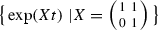
• 1. The curve $y=x^\alpha ,x>0,\alpha \notin \{0,1,\frac{1}{2},2\}$ is the orbit of the one-parameter subgroup ,

• 2. The curve $y=x\ln x$ is the orbit of the one-parameter subgroup ,

• 3. The logarithmic spiral with polar coordinates $\displaystyle \rho =\exp \big (\frac{\alpha }{\beta }\theta \big )$, where $\displaystyle \beta =\frac{\sqrt{1-\alpha ^2}}{3}$ with $0\le \alpha <1$ is the orbit of the one-parameter subgroup .

Remark 3.11

By Eqs. (3.7) and (3.9), the fully affine arc length element $\mathrm {d}\sigma$ can be expressed in terms of the equi-affine differential invariants as $\frac{\mathrm {d}\sigma }{\mathrm {d}\nu }= 3\sqrt{|\mu |},$ where $\nu$ is the equi-affine arc length element and $\mu$ is the equi-affine curvature. Then from Eqs. (3.7) and (3.15), the fully affine curvature can be written in terms of the equi-affine curvature and its derivatives as $\left( \tfrac{1}{\sqrt{|\mu |}}\right) _\nu$. Furthermore, the affine arc length element $\mathrm {d}\sigma$ can be expressed in terms of the Euclidean arc length element s and differential invariants as $\frac{\mathrm {d}\sigma }{\mathrm {d}s}= \sqrt{\frac{|3\phi \phi _{ss}-5\phi ^2_s+9\phi ^4|}{\phi ^2}},$ where s is the Euclidean arc length element and $\phi$ is the Euclidean curvature. The fully affine curvature can be written in terms of the Euclidean curvature and its derivatives as: $\left| \frac{\phi _s}{\sqrt{|3\phi \phi _{ss}-5\phi ^2_s+9\phi ^4|}}+3\left( \sqrt{\frac{\phi ^2}{|3\phi \phi _{ss}-5\phi ^2_s+9\phi ^4|}}\right) _s\right| .$ In fact, according to [11], we have $\frac{\mathrm {d}\nu }{\mathrm {d}s}=\phi ^{\frac{1}{3}}$ and $\mu =\frac{3\phi \phi _{ss}-5\phi ^2_s+9\phi ^4}{9\phi ^{\frac{8}{3}}}$.

4 Moving Frame Construction for the Affine Group that Factors as a Product

In fact, it will be simpler to construct the moving frames and then obtain differential invariants if the acting group has fewer parameters. Thus, it is desirable to use the results obtained for a subgroup $A\subset G$ to construct a moving frame and differential invariants for the entire group G. The inductive algorithms [10, 11] presented by Kogan allow us, in the case when the group G factors as a product, to extend a moving frame for a subgroup to the entire group. One also obtains at the same time the relations among the invariants of group G and its subgroup A. It is worth remarking that, in order to obtain such relations, the algorithm does not require the explicit formulae for the invariants of either G and A, but only the corresponding moving frames which lead to these invariants.

In this section, we use the algorithm [10, 11] to make an induction from the Euclidean action on plane curves to the affine action. Firstly, let us review the action of the special Euclidean group $SE(2)=SO(2) < imes \mathbb {R}^2$ on plane curve $u=u(x)$ [10, 11]. Its first prolongation, given by

$$\begin{aligned} y&=x\cos \alpha -u\sin \alpha +a,\nonumber \\ v&=x\sin \alpha +u\cos \alpha +b,\nonumber \\ v_y&=\frac{\sin \alpha +u_x\cos \alpha }{cos\alpha -u_x\sin \alpha }, \end{aligned}$$

(4.1)

defines a free action on $J^1(\mathbb {R}^2,1)$. We could get a moving frame on $J^1(\mathbb {R}^2,1)$ by choosing a cross section $\{x=0,u=0,u_x=0\}$. Then by setting $\{y=0,v=0,v_y=0\}$, it is simple to find an equivariant map $J^1(\mathbb {R}^2,1)\rightarrow SE(2)$

$$\begin{aligned} \alpha =-\arctan u_x, \ \ a=-\frac{u_xu+x}{\sqrt{1+u^2_x}},\ \ b=\frac{u_xx-u}{\sqrt{1+u^2_x}}. \end{aligned}$$

(4.2)

Therefore, the corresponding element of the special Euclidean group can be written in a matrix form

$$\begin{aligned} \rho = \left( \begin{array}{ccc} \frac{1}{\sqrt{1+u^2_x}} &{} \frac{u_x}{\sqrt{1+u^2_x}} &{} -\frac{uu_x+x}{\sqrt{1+u^2_x}} \\ -\frac{u_x}{\sqrt{1+u^2_x}} &{} \frac{1}{\sqrt{1+u^2_x}} &{} \frac{xu_x-u}{\sqrt{1+u^2_x}} \\ 0 &{} 0 &{} 1 \\ \end{array} \right) . \end{aligned}$$

(4.3)

Then the following differential invariants can be obtained directly

$$\begin{aligned} I^e_2&=v_{yy}=\frac{u_{xx}}{(1+u^2_x)^{\frac{3}{2}}},\nonumber \\ I^e_3&=v_{yyy}=\frac{(1+u^2_x)u_{xxx}-3u_xu^2_{xx}}{(1+u^2_x)^3},\\ I^e_4&=v_{yyyy}=\frac{(1+u^2_x)^2u_{xxxx}-10u_xu_{xx}u_{xxx}(1+u^2_x)+15u^2_xu^3_{xx}}{(1+u^2_x)^\frac{9}{2}}.\nonumber \end{aligned}$$

(4.4)

Now we denote by $I^e_2=\kappa$ the Euclidean curvature. Immediately, from the recurrence formula (2.7) , we have

$$\begin{aligned} I^e_3&=\kappa _s,\nonumber \\ I^e_4&=\kappa _{ss}+3\kappa ^3,\\ I^e_5&=\kappa _{sss}+19\kappa ^2\kappa _s,\nonumber \end{aligned}$$

(4.5)

where $\mathrm {d}s=\sqrt{1+u^2_x}\mathrm {d}x$ is infinitesimal Euclidean arc length. The contact invariant differential form equals to $\omega =\sqrt{1+u^2_x}\mathrm {d}x=\mathrm {d}s$. The dual total vector field $\mathcal {D}=\frac{1}{\sqrt{1+u^2_x}}D_x=\frac{\mathrm {d}}{\mathrm {d}s}$ provides an invariant differential operator, and any other invariant can be expressed as a function of $I^e_2$ and its derivatives with respect to $\mathcal {D}$.

Now it is time to build a moving frame for the affine group, by using the moving frame obtained above for the special Euclidean group SE$(2,\mathbb {R})$ acting on curves in $\mathbb {R}^2$. Obviously, the affine group transformation GA$(2,\mathbb {R})$ on the plane is the semi-direct product of the general linear group GL$(2,\mathbb {R})$ and translations in $\mathbb {R}^2$. Thus, we prolong it to the first jet bundle and notice that the isotropy group B of the point $z^{(1)}_0=\{x=0,u=0,u_x=0\}$ is given by all linear transformations of the form

$$\begin{aligned} \left( \begin{array}{cc} \alpha &{}\quad \beta \\ 0 &{}\quad \delta \\ \end{array} \right) , \end{aligned}$$

(4.6)

where $\alpha \delta \ne 0$. Thus, $GA(2,\mathbb {R})=B\cdot SE(2,\mathbb {R})$ and $B\cap SE(2,R)$ is finite. Exactly $B\cap SE(2,R)=\{I,-I\}$. Then let us prolong the action of B up to fifth order:

$$\begin{aligned} y&=\alpha x+\beta u,\\ v&=\delta u,\\ v_y&=\frac{\delta u_x}{\alpha +\beta u_x},\\ v_{yy}&=\frac{\alpha \delta u_{xx}}{(\alpha +\beta u_x)^3},\\ v_{yyy}&=\frac{\alpha \delta (\alpha +\beta u_x)u_{xxx}-3\alpha \beta \delta u^2_{xx}}{(\alpha +\beta u_x)^5},\\ v_{yyyy}&=\frac{\alpha \delta (\alpha +\beta u_x)^2u_{xxxx}-10\alpha \beta \delta u_{xx}u_{xxx}(\alpha +\beta u_x)+15\alpha \beta ^2\delta u^3_{xx}}{(\alpha +\beta u_x)^7},\\ v_{yyyyy}&=\frac{A}{(\alpha +\beta u_x)^9}, \end{aligned}$$

where

$$\begin{aligned} A=&\,\alpha \delta (\alpha +\beta u_x)^3u_{xxxxx}-15\alpha \beta \delta u_{xx}u_{xxxx}(\alpha +\beta u_x)^2-10\alpha \beta \delta u^2_{xxx}(\alpha +\beta u_x)^2\\&+105\alpha \beta ^2\delta u^2_{xx}u_{xxx}(\alpha +\beta u_x)-105\alpha \beta ^3\delta u^4_{xx}. \end{aligned}$$

If we restrict these transformations to the Euclidean cross section

$$\begin{aligned} \mathcal {K}^5_E=\{z^{(5)}\mid \pi ^5_1(z^{(5)})=z^{(1)}_0\}=\{z^{(5)}\mid x=0, u=0,u_x=0\}, \end{aligned}$$

then it follows that

$$\begin{aligned} v_{yy}=\,&\delta \frac{u_{xx}}{\alpha ^2},\\ v_{yyy}=\,&\delta \frac{\alpha u_{xxx}-3\beta u^2_{xx}}{\alpha ^4},\\ v_{yyyy}=\,&\delta \frac{\alpha ^2u_{xxxx}-10\alpha \beta u_{xx}u_{xxx}+15\beta ^2u^3_{xx}}{\alpha ^6},\\ v_{yyyyy}=\,&\delta \frac{\alpha ^3u_{xxxxx}-15\alpha ^2\beta u_{xx}u_{xxxx}-10\alpha ^2\beta u^2_{xxx}+105\alpha \beta ^2u^2_{xx}u_{xxx}-105\beta ^3u^4_{xx}}{\alpha ^8}. \end{aligned}$$

In fact, the above action is free on the open subset $\{z^{(5)}\in \mathcal {K}^5_E\mid u_{xx}\ne 0\}$. The cross section

$$\begin{aligned} \mathcal {K}^5=\left\{ z^{(5)}\in \mathcal {K}^5_E\mid u_{xx}=\frac{9}{2},\ \ u_{xxx}=0,\ \ u_{xxxx}=\frac{3}{2}\right\} \end{aligned}$$

to the orbit of B on $\mathcal {K}^5_E$ can generate a moving frame $\rho _B:\mathcal {K}^5_E\rightarrow B$:

$$\begin{aligned} \alpha ^2=\frac{3u_{xx}u_{xxxx}-5u^2_{xxx}}{u^2_{xx}}, \ \ \beta =\frac{\alpha u_{xxx}}{3u^2_{xx}},\ \ \delta =\frac{9\alpha ^2}{2u_{xx}}. \end{aligned}$$

Thus, we obtain the corresponding fifth-order invariant for the action of B on $\mathcal {K}^5_E$

$$\begin{aligned} I^b_5=\frac{9}{2}\frac{u^2_{xx}u_{xxxxx}-5u_{xx}u_{xxx}u_{xxxx}+\frac{40}{9}u^3_{xxx}}{(3u_{xx}u_{xxxx}-5u^2_{xxx})^\frac{3}{2}}, \end{aligned}$$

(4.7)

which is the affine curvature in Eqs. (3.17) and (2.13).

It is clear that $\mathcal {K}^5$ is a cross section to the orbits of the entire group $GA(2,\mathbb {R})$ on the open subset of $J^5$ where $u_{xx}\ne 0$. Then the fifth-order affine invariant can be obtained by invariantization of $I^b_5$ with respect to Euclidean action. So we get the lowest order affine invariant $\mu$ according to Euclidean invariants

$$\begin{aligned} \mu =I^a_5=\frac{9\left( (I^e_2)^2I^e_5-5I^e_2I^e_3I^e_4+\frac{40}{9}(I^e_3)^3\right) }{2(3I^e_2I^e_4-5(I^e_3)^2)^{\frac{3}{2}}}. \end{aligned}$$

(4.8)

This equation can be rewritten by using the Euclidean curvature $I^e_2=\kappa$ and its derivatives in Eq. (4.5). The moving frame for the affine group corresponding to the cross section $\mathcal {K}^5$ is the product of two matrices

$$\begin{aligned} \left( \begin{array}{ccc} \frac{\sqrt{3u_{xx}u_{xxxx}-5u^2_{xxx}}}{u_{xx}} &{}\quad \frac{u_{xxx}\sqrt{3u_{xx}u_{xxxx}-5u^2_{xxx}}}{3u^3_{xx}} &{}\quad 0 \\ 0 &{}\quad \frac{9(3u_{xx}u_{xxxx}-5u^2_{xxx})}{2u^3_{xx}} &{}\quad 0 \\ 0 &{}\quad 0 &{}\quad 1 \\ \end{array} \right) \left( \begin{array}{ccc} \frac{1}{\sqrt{1+u^2_x}} &{}\quad \frac{u_x}{\sqrt{1+u^2_x}} &{}\quad -\frac{uu_x+x}{\sqrt{1+u^2_x}} \\ -\frac{u_x}{\sqrt{1+u^2_x}} &{}\quad \frac{1}{\sqrt{1+u^2_x}} &{}\quad \frac{xu_x-u}{\sqrt{1+u^2_x}} \\ 0 &{}\quad 0 &{}\quad 1 \\ \end{array} \right) . \end{aligned}$$

(4.9)

We can obtain the affine contact invariant horizontal form $\mathrm {d}\theta$ in terms of the Euclidean arc length $\mathrm {d}s$ (see [10, 11] for the detailed definitions of the notations):

$$\begin{aligned} \mathrm {d}\theta =\sigma ^*_B\sigma ^*_E\pi _H\omega ^*_E\mathrm {d}_H\omega ^*_E(x), \end{aligned}$$

where the Euclidean invariantization of $\mathrm {d}_H\omega ^*_B(x)=(\alpha +\beta u_x)\mathrm {d}x$ equals to $\alpha \mathrm {d}s$ and hence

$$\begin{aligned} \mathrm {d}\theta =\sigma ^*_B(\alpha \mathrm {d}s)=\frac{\sqrt{3I^e_2I^e_4-5(I^e_3)^2}}{I^e_2}\mathrm {d}s. \end{aligned}$$

(4.10)

The form $\mathrm {d}\theta$ is the affine arc length and can be written in the standard coordinates as

$$\begin{aligned} \mathrm {d}\theta =\frac{\sqrt{3u_{xx}u_{xxxx}-5u^2_{xxx}}}{u_{xx}}\mathrm {d}x, \end{aligned}$$

which is coincident to Eq. (2.12).

5 Applications of Affine Curvature

In this section, we will employ the affine curvature defined in the previous sections to determine whether two smooth (or discrete) planar curves are affine equivalent. Furthermore, once we can confirm that the two smooth (or discrete) curves are affine equivalent, the least squares method will be utilized for identifying the most suitable affine transformation between them. After applying the affine transformation to transform one of the two curves, the accuracy can be calculated and evaluated. In Sect.  5.1, we introduce a numerical algorithm to assess the degree of equivalence between two planar curves. In Sect.  5.2, the affine signature curves will be applied to judge whether there exist an affine transformation between two smooth planar curves. In Sect. 5.3, the discrete case is considered.

5.1 Measuring Numerically How Well Two Curves Match

As we know, the inner product between two (sufficiently nice) functions f(x) and g(x) over the interval [a, b],

$$\begin{aligned} \langle f(x),g(x) \rangle :=\int ^b_cf(x)g(x)\mathrm {d}x, \end{aligned}$$

often is considered as a standard way to compare the degree of equivalence between these two functions, and from which we get

$$\begin{aligned} ||f(x)-g(x)||=\sqrt{\int ^b_a(f(x)-g(x))^2\mathrm {d}x}, \end{aligned}$$

where $||f(x)-g(x)||$ can be defined as the distance between the functions f(x) and g(x), and denoted by $\mathrm {dist}(f(x),g(x))$. Thus, if $\mathrm {dist}(f(x),g(x))=0$, immediately we can conclude that

$$\begin{aligned} f(x)\equiv g(x),\ \ \forall x\in [a,b]. \end{aligned}$$

Now we can apply this concept to compare two discrete curves. Let us say, the curve A consists of N points and all the points are

$$\begin{aligned} (x_{a_1}, y_{a_1})^{\mathrm{Trans}},~(x_{a_2}, y_{a_2})^{\mathrm{Trans}},~\ldots , ~(x_{a_N}, y_{a_N})^{\mathrm{Trans}}. \end{aligned}$$

Similarly, the curve B consists of M points

$$\begin{aligned} (x_{b_1}, y_{b_1})^{\mathrm{Trans}},~(x_{b_2}, y_{b_2})^{\mathrm{Trans}},~\ldots , ~(x_{b_M}, y_{b_M})^{\mathrm{Trans}}. \end{aligned}$$

Locally, we can always assume that $x_{a_1}<x_{a_2}<\cdots <x_{a_N}$ and $x_{b_1}<x_{b_2}<\cdots <x_{b_M}$. For the sake of convenience, we take the following notations to indicate the maps of Curve A and Curve B, that is,

$$\begin{aligned} y_{a_i}=f(x_{a_i}), \ \ y_{b_j}=g(x_{b_j}),\ \ i=1,2,\ldots ,N,\ \ j=1,2,\ldots ,M. \end{aligned}$$

Two new sets $\{x'_{a_i}\}$ and $\{x'_{b_i}\}$ of x-coordinates are created by choosing $x'_{a_i}\in \{x_{a_i}\}$ and $x'_{b_i}\in \{x_{b_i}\}$ such that $x'_{a_1}<x'_{b_1}<x'_{a_2}<x'_{b_2}<\cdots$ or $x'_{b_1}<x'_{a_1}<x'_{b_2}<x'_{a_2}<\cdots$. Then, we need to generate a common set of points for both curves with x-coordinates from the following set.

$$\begin{aligned} \{x_1,x_2,\ldots ,x_K\}=\{x'_{a_1},x'_{a_2},\ldots ,x'_{a_{N'}}\}\cup \{x'_{b_1},x'_{b_2},\ldots ,x'_{b_{M'}}\}, \end{aligned}$$

where $x_1<x_2<\cdots <x_K$ and $\max \{M',N'\}\le K\le M'+N'$. The next step is to define the maps for the set $\{x_1,x_2,\cdots ,x_K\}$, and here we take

$$\begin{aligned} f(x_i)= \left\{ \begin{array}{ll} \frac{(x_i-x'_{a_{l-1}})f(x'_{a_l})+(x'_{a_l}-x_i)f(x'_{a_{l-1}})}{x'_{a_l}-x'_{a_{l-1}}}, &{} x'_{a_{l-1}}\le x_i\le x'_{a_l}, \ \ 1<l\le N', \\ g(x_i)&{} x_i<x'_{a_1}, \\ g(x_i)&{} x_i>x'_{a_{N'}}, \end{array} \right. \end{aligned}$$

(5.1)

and

$$\begin{aligned} g(x_i)= \left\{ \begin{array}{ll} \frac{(x_i-x'_{b_{l-1}})g(x'_{b_l})+(x'_{b_l}-x_i)g(x'_{b_{l-1}})}{x'_{b_l}-x'_{b_{l-1}}}, &{} x'_{b_{l-1}}\le x_i\le x'_{b_l}, \ \ 1<l\le M', \\ f(x_i)&{} x_i<x'_{b_1}, \\ f(x_i)&{} x_i>x'_{b_{M'}}. \end{array} \right. \end{aligned}$$

(5.2)

The missing y-coordinates (if any) for each curve are obtained via interpolating neighboring points. Notice that in the second and third entries, f and g are reversed. For the new function f(x), if $x_i<x'_{a_1}$ or $x_i>x'_{a_N}$, then $x_i$ is the first one or last one. So $x_i\in \{x'_{b_i}\}$, and we take its value from g(x). The same operation is performed for the new function g(x). Thus, we can calculate the difference between Curve A and Curve B by

$$\begin{aligned} \mathrm {dist}_1=\max \{|f(x_i)-g(x_i)|, i=1,2,\ldots ,K\}\ \ \mathrm {or}\ \ \mathrm {dist}_2=\frac{1}{K}\sqrt{\sum ^K_{i=1}|f(x_i)-g(x_i)|^2}. \end{aligned}$$

(5.3)

The value of difference rate can be given by

$$\begin{aligned} \mathrm {error}_1=\frac{\mathrm {dist}_1}{\displaystyle \frac{1}{N}\sum \nolimits ^N_{i=1}|y_{a_i}|} \ \ \mathrm {or} \ \ \mathrm {error}_2=\frac{\mathrm {dist}_2}{\displaystyle \frac{1}{N}\sqrt{\sum \nolimits ^N_{i=1}y^2_{a_i}}}. \end{aligned}$$

(5.4)

Remark 5.1

The possible signature metrics for comparison of digital signatures are Hausdorff, Monge–Kantorovich transport, electrostatic repulsion, latent semantic analysis, histograms, geodesic distance, diffusion metric, Gromov–Hausdorff, etc [1, 2]. In [8], Hoff and Olver used signature similarity coefficient to measure the closeness of the two signatures. In this paper, in order to simple show the practicability of the signature curve in matching curves up to an affine transformation, we directly use the $L^2$ inner product and norm to compare signatures. Practical issues require the appropriate metric to compare signatures, which is an important issue we are studying.

5.2 Detecting the Affine Equivalence Between Two Smooth Planar Curves

On the basis of the previous sections, it is clear that, by a certain generating set of invariants and a collection of invariant differential operators, all of the essential differential invariants can be produced, while the differential invariants often are used to find the global equivalence of two curves and symmetries of the curve. Certainly, the equivalence and symmetry problem can be solved using the signature curves [9, 18, 22]. As introduced in Sect. 2.1, S is the submanifold of manifold M. Let n be the order of stabilization of the group action and $\{I_1,I_2,\ldots , I_{N_k}\}$ be a complete list of differential invariants for any $k\ge n$. The restriction of the invariants to the k-jet of S, $j^kS$, is denoted by $\tilde{I}_\alpha =I_{\alpha }|_{J^kS}$, and we define $\phi ^k:S\rightarrow \{\tilde{I}_1,\ldots ,\tilde{I}_{N_k}\}$. Accordingly, the $k^{\mathrm{th}}$-order signature curve$\mathcal {C}^k$ of the submanifold S is the immersed manifold $Im(\phi ^k)\subset \mathbb {R}^{N_k}$.

In fact, if two curves $C_1$ and $C_2$ are affine equivalent, they have same $\kappa =|\kappa _2|,\epsilon , (\kappa _2)_\sigma$ appearing in Eqs. (3.14), (3.15) and (3.18). Hence, the curves $(\kappa ,\epsilon )$ and $(\kappa ,(\kappa _2)_\sigma )$ generated by curves $C_1$ and $C_2$ are same. On the contrary, $\epsilon , \kappa$ decide a unique curve up to an affine transformation from Theorem 3.6. If we have exact functions for $(\kappa ,\epsilon )$ and $(\kappa ,(\kappa _2)_\sigma )$, the curve can be identified uniquely up to an affine transformation. Thus, the curves $(\kappa ,\epsilon )$ and $(\kappa ,(\kappa _2)_\sigma )$ are considered as the affine signature curves.

In the following, through an example, we elaborate the process to assess the affine equivalence of two curves and identify the affine transformation between them.

Example 5.2

Firstly, we list three parametric curves expressed by the following equations

$$\begin{aligned} \mathbf {x}_1(t)= & {} \left( \begin{array}{c} \cos t+\cos 2t+\cos 3t \\ \sin t-\sin 2t-\sin 3t \\ \end{array} \right) ,\qquad 0< t< \pi , \end{aligned}$$

(5.5)

$$\begin{aligned} \mathbf {x}_2(t)= & {} \left( \begin{array}{c} (2-t)(1-t)(1-2t) \\ (2-t)(1-2t)\sqrt{8t-t^4} \\ \end{array} \right) ,\qquad 0< t< 2, \end{aligned}$$

(5.6)

and

$$\begin{aligned} \mathbf {x}_3(t)=\left( \begin{array}{c} 8t^3-14t^2+7t \\ (4t^2-5t+1)(\sqrt{t-t^2}+0.5(1-2t)) \\ \end{array} \right) ,\qquad 0< t< 1. \end{aligned}$$

(5.7)

Our goal is to make sure whether there are some affine transformations between them. Generally, we should first draw graphs of these curves which can clearly show topological and geometrical properties. Sometimes, we can know two curves are not affine equivalent directly from their graphs according to the properties preserved by the affine transformation.

Fig. 1

The images of the curves

Definitely, their graphs are shown in Fig. 1. However, in this example, directly observing the graphs in Fig. 1, it is difficult to determine affine equivalence among them.

Thus, we need to further investigate their signature curves which are shown in Figs. 2 and 3. In Fig. 2, these three graphs are almost same. But in Fig. 3, we do not hesitate to tell that the curve $\mathbf {x}_2(t)$ can not be affine equivalent to either of the two curves $\mathbf {x}_1(t)$ and $\mathbf {x}_3(t)$, since the middle graphs of Fig. 3 look obviously different from the other two. Of course, it seems that the left and right of Fig. 3 are the same.

Fig. 2

The relations between $\kappa$ and $\epsilon$

Fig. 3

The relations between $(\kappa _2)_\sigma$ and $\kappa$

With the help of Figs. 2 and 3, the possibility of the curve $\mathbf {x}_2(t)$ is excluded, and we could move ahead to estimate if there exist an affine transformation between $\mathbf {x}_1(t)$ and $\mathbf {x}_3(t)$.

By a direct computation, we obtain both maximum values of $\kappa$ for the curves $\mathbf {x}_1(t)$ and $\mathbf {x}_3(t)$ are the same value 2.5. At the same time, according to Eqs. (3.8) and (3.14), $\epsilon$ is constant for a non-degenerate affine curve. Thus, it is obvious that the left and right of Fig. 2 are totally the same.

In order to verify the left and right of Fig. 3 are the same graph, we need to use the method stated in Sect.  5.1. Exactly, if they are same, we can conclude that the two curves $\mathbf {x}_1(t)$ and $\mathbf {x}_3(t)$ are affine equivalent, and we will further obtain the affine transformation between them from some corresponding points.

Let us first calculate the difference and the value of difference rate in Eqs. (5.3) and (5.4) between the left and the right pictures in Fig. 3. According to the signature curves in Fig. 3, we should divide them into seven parts on the basis of the monotonicity marked by different colors in Fig. 3. By careful comparison and analysis, it is easy to obtain the ranges of parameter t for these seven parts which are listed in Table 2.

Table 2 The ranges of parameter t for seven parts

Then we choose 50001 points at each part of s1, s2,$\ldots$ s7 in Fig. 3. Using the method stated in Sect.  5.1, we obtain the difference and the value of difference rate for these seven parts which are shown in Table 3.

Table 3 The distances and errors for seven parts

From the data listed in Table 3, it is apparent that all the values are very small and almost zero. If we increase the number of points, all the values in Table 3 will further decrease. Inevitably, there are some errors in numerical calculation and the values for difference rate are considered to be within acceptable limits, so we can conclude that the curves $\{\mathbf {x}_1(t), 0<t<\pi \}$ and $\{\mathbf {x}_3(t), 0<t<1\}$ are affine equivalent.

Now let us search for the affine transformation between the curves $\mathbf {x}_1(t)$ and $\mathbf {x}_3(t)$. According to the method and Eqs. (5.1)–(5.2) in Sect. 5.1, we have obtained three series

$$\begin{aligned}&\{\kappa _1,\kappa _2,\ldots ,\kappa _K\},\\&\{f(\kappa _1),f(\kappa _2),\ldots ,f(\kappa _K)\}, \end{aligned}$$

and

$$\begin{aligned} \{g(\kappa _1),g(\kappa _2),\ldots ,g(\kappa _K)\}. \end{aligned}$$

At the same time, it is easy to collect the values $(t_1)_i\in (0,\pi )$ and $(t_2)_i\in (0,1)$ which correspond to the curvature $\kappa _i, i=1,2,\ldots ,K$ for curves $\mathbf {x}_1(t)$ and $\mathbf {x}_3(t)$, respectively.

In order to compute it more accurately, we fix a small number e and choose these corresponding points $(t_1)_i$ and $(t_2)_i$ which satisfying the condition $|f(\kappa _i)-g(\kappa _i)|<e$. In the above case, if we choose $e=10^{-8}$, we still gain 634793 points which satisfy the condition.

Since there exists an affine transformation between $\{\mathbf {x}_1(t), 0<t<\pi \}$ and $\{\mathbf {x}_3(t), 0<t<1\}$ from above analysis, we assume

$$\begin{aligned} \mathbf {x}_1(t_1)= \left( \begin{array}{cc} a &{} b \\ c &{} d \\ \end{array} \right) \mathbf {x}_3(t_2) +\left( \begin{array}{c} e \\ f\\ \end{array} \right) ,\ \ 0<t_1<\pi ,\ \ 0<t_2<1, \end{aligned}$$

(5.8)

which implies

$$\begin{aligned} \left( \begin{array}{cccccc} (\mathbf {x}_3(t_2))_x &{}(\mathbf {x}_3(t_2))_y &{} 0&{} 0&{} 1 &{} 0 \\ 0&{}0&{}(\mathbf {x}_3(t_2))_x &{}(\mathbf {x}_3(t_2))_y&{} 0&{}1\\ \end{array} \right) \left( \begin{array}{c} a \\ b \\ c \\ d \\ e \\ f \\ \end{array} \right) = \left( \begin{array}{c} (\mathbf {x}_1(t_1))_x \\ (\mathbf {x}_1(t_1))_y\\ \end{array} \right) , \end{aligned}$$

(5.9)

where $(\mathbf {x})_x, (\mathbf {x})_y$ denote the x-coordinate and y-coordinate of the vector $\mathbf {x}$, respectively. Then using the least square method at the corresponding points $(t_1)_i$ and $(t_2)_i$ which satisfying that $|f(\kappa _i)-g(\kappa _i)|<e$, we can get the most suitable solution for the parameters a, b, c, d, e, f.

In the above case, there are more than 508210 points which satisfy the condition. Then using them and the least square method, we can find that the solution of the parameters a, b, c, d, e, f is

$$\begin{aligned}&a=-4.0000000,~b=0.0000000,~ c=-4.0000000,~ d=-8.0000000,\nonumber \\&e=3.0000000,~ f=4.0000000. \end{aligned}$$

(5.10)

Now by using these parameters, we transform the middle graph $\mathbf {x}_3(t), 0<t<1$ to the right graph of Fig. 4 and then compare it with the original graph $\mathbf {x}_1(t), 0<t<\pi$ as shown in the left of Fig. 4.

Fig. 4

Comparison between $\mathbf {x}_1(t)$ and $\mathbf {x}_3(t)$ after the affine transformation

Exactly, to make sure the left graph and the right graph of Fig. 4 are the same, we still need to use the method stated in Sect. 5.1. According to the monotonicity as shown in Fig. 4, it is better to divide it into three parts. By a careful calculation, we can obtain the ranges of t for Parts c1, c2 and c3 in Fig. 4 and the results are shown in Table 4.

Table 4 The ranges of t for c1, c2 and c3 in Fig. 4

In each unit-length interval of x-axis, we choose 600001 points as an example. By using the method stated in Sect. 5.1, we obtain the distances and errors in Eqs. (5.3) and (5.4) between the left graph and the right graph of Fig. 4 which are shown in Table 5.

Table 5 The distances and errors between the left and right (Fig. 4)

Remark 5.3

It seems that the results of Part c3 in Table 5 are slightly bigger than these of Part c1 and Part c2, and that is because some sections in Part c3 are abrupt with respect to x-axis, which is unfavorable for interpolation. In fact, in this part, the relation of x values and y values is the one-to-one correspondence for $\mathbf {x}_1(t)$ and the transformation of $\mathbf {x}_3(t)$. Then if we exchange x and y axis, the desired effects of Part c3 are discernible, which are

$$\begin{aligned}&\mathrm {dist}_1=2.7672\times 10^{-09},~\mathrm {dist}_2=6.9579\times 10^{-15},~\mathrm {error}_1=7.7556\times 10^{-09}, \\&\mathrm {error}_2=1.4592\times 10^{-11}. \end{aligned}$$

To sum up, the above result again shows that there exists an affine transformation between $\mathbf {x}_1(t), \ \ 0<t<\pi$ and $\mathbf {x}_3(t), \ \ 0<t<1$.

5.3 Applying the Affine Curvatures to the Discrete Point Sequence

In this part, we first prove that the fitting cubic curve of a discrete point set is affine invariant under an affine transformation, and then identify the discrete points with the affine curvatures along the fitting cubic curves.

Given n points in the plane, represented as $(x_1, y_1)^{\mathrm{Trans}},(x_2, y_2)^{\mathrm{Trans}},\cdots ,(x_n, y_n)^{\mathrm{Trans}}$, which generate a matrix

$$\begin{aligned} M_1= \left( \begin{array}{c@{\quad }c@{\quad }c@{\quad }c@{\quad }c@{\quad }c@{\quad }c@{\quad }c@{\quad }c@{\quad }c} x^3_1 &{} x^2_1y_1 &{} x_1y^2_1 &{} y^3_1 &{} x^2_1 &{} x_1y_1 &{} y^2_1 &{} x_1 &{} y_1 &{} 1 \\ x^3_2 &{} x^2_2y_2 &{} x_2y^2_2 &{} y^3_2 &{} x^2_2 &{} x_2y_2 &{} y^2_2 &{} x_2 &{} y_2 &{} 1 \\ \vdots &{} \vdots &{} \vdots &{} \vdots &{} \vdots &{} \vdots &{} \vdots &{} \vdots &{} \vdots &{} \vdots \\ x^3_n &{} x^2_ny_n &{} x_ny^2_n &{} y^3_n &{} x^2_n &{} x_ny_n &{} y^2_n &{} x_n &{} y_n &{} 1 \\ \end{array} \right) . \end{aligned}$$

(5.11)

Suppose $\mathbf {v}_1,\mathbf {v}_2, \cdots , \mathbf {v}_{10}$ are the ten column vectors of the matrix $M_1$, that is,

$$\begin{aligned} M_1=(\mathbf {v}_1\ \ \mathbf {v}_2\ \ \mathbf {v}_3\ \ \mathbf {v}_4\ \ \mathbf {v}_5\ \ \mathbf {v}_6\ \ \mathbf {v}_7\ \ \mathbf {v}_8\ \ \mathbf {v}_9\ \ \mathbf {v}_{10}). \end{aligned}$$

(5.12)

Thus, another matrix $M_2$ can be constructed by using these column vectors, and

$$\begin{aligned} M_2=\left( \mathbf {v}_5\ \ \mathbf {v}_6\ \ \mathbf {v}_7\ \ \mathbf {v}_8\ \ \mathbf {v}_9\ \ \mathbf {v}_{10}\right) . \end{aligned}$$

(5.13)

In particular, we can prove that

Theorem 5.4

If the ranks of the matrices $M_1$ and $M_2$ satisfy that

$$\begin{aligned} \mathrm {rank}(M_1)=9,\ \ \mathrm {rank}(M_2)=6, \end{aligned}$$

(5.14)

then there exists a unique cubic curve

$$\begin{aligned}&A_1x^3+A_2x^2y+A_3xy^2+A_4y^3+A_5x^2+A_6xy+A_7y^2+A_8x+A_9y+A_{10}=0,\nonumber \\&A^2_1+A^2_2+A^2_3+A^2_4\ne 0 \end{aligned}$$

(5.15)

passing through these n points $(x_1, y_1)^{\mathrm{Trans}},(x_2, y_2)^{\mathrm{Trans}},\cdots ,(x_n, y_n)^{\mathrm{Trans}}$.

Proof

Since $\mathrm {rank}(M_2)=6$, the solution vector $(A_5,A_6,\cdots , A_{10})$ of the equations

$$\begin{aligned} A_5x^2_i+A_6x_iy_i+A_7y^2_i+A_8x_i+A_9y_i+A_{10}=0,\ \ i=1,2,\ldots ,n \end{aligned}$$

is $A_5=A_6=\cdots =A_{10}=0$.

On the other hand, $\mathrm {rank}(M_1)=9$ implies that the unit vector $(A_1,A_2,\cdots ,A_{10})$ satisfying the equations

$$\begin{aligned}&A_1x^3_i+A_2x^2_iy_i+A_3x_iy^2_i+A_4y^3_i+A_5x^2_i+A_6x_iy_i+A_7y^2_i\\&\quad +A_8x_i+A_9y_i+A_{10}=0, \ \ i=1,2,\cdots ,n \end{aligned}$$

is unique up to a sign. Therefore, it is obvious that the conclusion of this theorem holds. $\square$

Let us consider an affine transformation

$$\begin{aligned} \begin{array}{l} x=\lambda _1x'+\lambda _2y'+\lambda _3\\ y=\lambda _4x'+\lambda _5y'+\lambda _6 \end{array} \ \ ,\qquad \ \ \mathrm {where} \ \ \lambda _1\lambda _5-\lambda _2\lambda _4\ne 0, \end{aligned}$$

(5.16)

on a plane. Clearly, by a computation, the relation between $\left( \mathbf {v}_1,\mathbf {v}_2,\cdots ,\mathbf {v}_{10}\right)$ and $\left( \mathbf {v}'_1,\mathbf {v}'_2,\cdots ,\mathbf {v}'_{10}\right)$ follows

$$\begin{aligned} \left( \mathbf {v}_1,\mathbf {v}_2,\ldots ,\mathbf {v}_{10}\right) =\left( \mathbf {v}'_1,\mathbf {v}'_2,\cdots ,\mathbf {v}'_{10}\right) \left( \begin{array}{c@{\quad }c@{\quad }c@{\quad }c} N &{} \mathbf {0} &{} \mathbf {0} &{} \mathbf {0} \\ N_2 &{} N_1 &{} \mathbf {0} &{} \mathbf {0} \\ N_3 &{} N_4 &{} N_5 &{} \mathbf {0} \\ N_6 &{} N_7 &{} N_8 &{} 1 \\ \end{array} \right) , \end{aligned}$$

(5.17)

where

$$\begin{aligned} N&= \left( \begin{array}{c@{\quad }c@{\quad }c@{\quad }c} \lambda ^3_1 &{} \lambda ^2_1\lambda _4 &{} \lambda ^2_4\lambda _1 &{} \lambda ^3_4 \\ 3\lambda ^2_1\lambda _2 &{} \lambda ^2_1\lambda _5+2\lambda _1\lambda _2\lambda _4 &{} \lambda ^2_4\lambda _2+2\lambda _1\lambda _4\lambda _5 &{} 3\lambda ^2_4\lambda _5 \\ 3\lambda _1\lambda ^2_2 &{} \lambda ^2_2\lambda _4+2\lambda _1\lambda _2\lambda _5 &{} \lambda _1\lambda ^2_5+2\lambda _2\lambda _4\lambda _5 &{} 3\lambda _4\lambda ^2_5 \\ \lambda ^3_2 &{} \lambda ^2_2\lambda _5 &{} \lambda ^2_5\lambda _2 &{} \lambda ^3_5 \\ \end{array} \right) , \\ N_1&= \left( \begin{array}{c@{\quad }c@{\quad }c} \lambda ^2_1 &{} \lambda _1\lambda _4 &{} \lambda ^2_4\\ 2\lambda _1\lambda _2 &{} \lambda _1\lambda _5+\lambda _2\lambda _4 &{} 2\lambda _4\lambda _5 \\ \lambda ^2_2 &{} \lambda _2\lambda _5 &{} \lambda ^2_5 \\ \end{array} \right) , \\ N_2&= \left( \begin{array}{c@{\quad }c@{\quad }c@{\quad }c} 3\lambda ^2_1\lambda _3 &{} \lambda ^2_1\lambda _6+2\lambda _1\lambda _3\lambda _4 &{} \lambda _3\lambda ^2_4+2\lambda _1\lambda _4\lambda _6 &{} 3\lambda ^2_4\lambda _6 \\ 6\lambda _1\lambda _2\lambda _3 &{} 2(\lambda _1\lambda _2\lambda _6+\lambda _1\lambda _3\lambda _5+\lambda _2\lambda _3\lambda _4) &{} 2(\lambda _3\lambda _4\lambda _5+\lambda _2\lambda _4\lambda _6+\lambda _1\lambda _5\lambda _6) &{} 6\lambda _4\lambda _5\lambda _6 \\ 3\lambda ^2_2\lambda _3 &{} \lambda ^2_2\lambda _6+2\lambda _2\lambda _3\lambda _5 &{} \lambda _3\lambda ^2_5+2\lambda _2\lambda _5\lambda _6 &{} 3\lambda ^3_5\lambda _6 \\ \end{array} \right) , \\ N_3&= \left( \begin{array}{c@{\quad }c@{\quad }c@{\quad }c} 3\lambda _1\lambda ^2_3 &{} \lambda ^2_3\lambda _4+2\lambda _1\lambda _3\lambda _6 &{} \lambda _1\lambda ^2_6+2\lambda _3\lambda _4\lambda _6 &{} 3\lambda _4\lambda ^2_6 \\ 3\lambda _2\lambda ^2_3 &{} \lambda ^2_3\lambda _5+2\lambda _2\lambda _3\lambda _6 &{} \lambda _2\lambda ^2_6+2\lambda _3\lambda _5\lambda _6 &{} 3\lambda _5\lambda ^2_6 \\ \end{array} \right) ,\\ N_4&= \left( \begin{array}{c@{\quad }c@{\quad }c} 2\lambda _1\lambda _3 &{} \lambda _1\lambda _6+\lambda _3\lambda _4 &{} 2\lambda _4\lambda _6 \\ 2\lambda _2\lambda _3 &{} \lambda _2\lambda _6+\lambda _3\lambda _5 &{} 2\lambda _5\lambda _6 \\ \end{array} \right) , \\ N_5&= \left( \begin{array}{c@{\quad }c} \lambda _1 &{} \lambda _4 \\ \lambda _2 &{} \lambda _5 \\ \end{array} \right) , \ \ N_6= \left( \begin{array}{c@{\quad }c@{\quad }c@{\quad }c} \lambda ^3_3 &{} \lambda ^2_3\lambda _6 &{} \lambda _3\lambda ^2_6 &{} \lambda ^3_6 \\ \end{array} \right) , \ \ N_7= \left( \begin{array}{c@{\quad }c@{\quad }c} \lambda ^2_3 &{} \lambda _3\lambda _6 &{} \lambda ^2_6 \\ \end{array} \right) , \ \ N_8= \left( \begin{array}{c@{\quad }c} \lambda _3 &{} \lambda _6 \\ \end{array} \right) . \end{aligned}$$

Hence, it yields that

Theorem 5.5

A cubic curve

$$\begin{aligned}&A_1x^3+A_2x^2y+A_3xy^2+A_4y^3+A_5x^2+A_6xy+A_7y^2+A_8x+A_9y+A_{10}=0,\\&A^2_1+A^2_2+A^2_3+A^2_4\ne 0 \end{aligned}$$

is still a cubic curve under an affine transformation.

Let us also verify the following theorem.

Theorem 5.6

Assume two point sets $P=\{P_1,P_2,\ldots ,P_n\}$ and $Q=\{Q_1,Q_2,\ldots ,Q_n\}$ are affine equivalent, where $n\ge 9$. If the n points $P_1,P_2,\cdots ,P_n$ satisfy the conditions of Theorem 5.4, which determine uniquely a cubic curve $C_p$, then the n points $Q_1,Q_2,\cdots ,Q_n$ also determine uniquely a cubic curve $C_q$, and the cubic curves $C_p$ and $C_q$ are affine equivalent with the same correspondence as that between P and Q.

Proof

Under the affine transformation (5.16), we have the relation in Eq. (5.17). By a direct calculation, it appears that

$$\begin{aligned}&\det (N)=(\lambda _1\lambda _5-\lambda _2\lambda _4)^6\ne 0,\ \ \det (N_1)=(\lambda _1\lambda _5-\lambda _2\lambda _4)^3\ne 0,\\&\det (N_5)=\lambda _1\lambda _5-\lambda _2\lambda _4\ne 0. \end{aligned}$$

Then, again from Eq. (5.17), we can conclude that

$$\begin{aligned} \mathrm {rank}\left\{ \mathbf {v}_1,\mathbf {v}_2,\cdots ,\mathbf {v}_{10}\right\} =\mathrm {rank}\left\{ \mathbf {v}'_1,\mathbf {v}'_2,\cdots ,\mathbf {v}'_{10}\right\} \end{aligned}$$

and

$$\begin{aligned} \mathrm {rank}\left\{ \mathbf {v}_5,\mathbf {v}_6,\cdots ,\mathbf {v}_{10}\right\} =\mathrm {rank}\left\{ \mathbf {v}'_5,\mathbf {v}'_6,\cdots ,\mathbf {v}'_{10}\right\} . \end{aligned}$$

Finally, combining of Theorem 5.4 and Theorem 5.5 yields the conclusion of this theorem. $\square$

Remark 5.7

In fact, by using the above method, we can consider further the similar conclusions for quartic curve, quintic curve, and so on. On the other hand, if $\mathrm {rank}(M_2)=6$ and $6\le \mathrm {rank}(M_1)<9$, there are more than one cubic curves passing through these points, and after an affine transformation, we need to verify them respectively.

Fig. 5

The comparison of signature curves between the smooth curve and the fitting cubic curves

Next let us consider how to describe the affine curvature of the discrete curve. Firstly, we fit piecewise the discrete points by using the cubic curves. In fact, it is convenient to find the derivatives of the implicit functions. Then according to Eqs. (3.16)-(3.18), we can obtain the affine invariants $\epsilon$, $\kappa$, $\frac{\mathrm {d}\kappa _2}{\mathrm {d}\sigma }$ of these points along the fitting cubic curve, and these points can be identified by the affine invariants $\epsilon$, $\kappa$, $\frac{\mathrm {d}\kappa _2}{\mathrm {d}\sigma }$. By this way, it is more convenient to find the correspondence relation between two affine equivalent point sets. In the following example, we show the relations of the affine curvatures among a smooth curve, the fitting cubic curves for the discrete points on this smooth curve and the fitting cubic curves for the smooth curve after an affine transformation.

Example 5.8

From Sect. 5.2, we know the curves $\{\mathbf {x}_1(t), 0<t<0.4180312\}$ and $\{\mathbf {x}_3(t), 0<t<0.04305502\}$ in Example 5.2 are affine equivalent. It is convenient to obtain some discrete points on these two curves. We choose 6000 equidistant points for parameter t on the intervals (0, 0.4180312) and (0, 0.04305502) and generate two discrete point sets $P_1$ and $P_2$ on the curves $\mathbf {x}_1(t)$ and $\mathbf {x}_3(t)$, respectively.

Next, we fit piecewise the discrete points in the sets $P_1$ and $P_2$ to the cubic curves by using Theorem 5.4 and calculate their smooth affine curvatures at every point along the fitting cubic curves. Their signature curves are shown in Fig. 5.

In every row of Fig. 5, the left ones are the signature curves of the smooth curve $\mathbf {x}_1(t)$, and the middle twos are the signature curves of the fitting cubic curves to the discrete point sequence $P_1$ and $P_2$. For the sake of direct comparison and contrast, we put the left three results together into one graph as shown in the right ones of Fig. 5. From the visual point of view in Fig. 5, it is no doubt that the fitting affine curvatures are very close to the origin affine curvatures on the curves $\mathbf {x}_1(t)$ and $\mathbf {x}_3(t)$ in Example 5.2, and the fitting effect is satisfactory. Of course, in order to obtain a more accurate result, we need to apply the similar numerical method as that used in Sect. 5.2 and find the affine transformation through those corresponding points whose affine curvatures are the nearest and by using the least square method mentioned in Sect. 5.2. Finally, we can compare the difference between one point set $P_1$ and the image of another point set $P_2$ after the affine transformation obtained.

References

Brinkman, D., Olver, P.J.: Invariant histograms. Am. Math. Mon. 119, 4–24 (2012)
Calabi, E., Olver, P.J., Shakiban, C., Tannenbaum, A., Haker, S.: Differential and numerically invariant signature curves applied to object recognition. Int. J. Comput. Vis. 26, 107–135 (1998)
Chou, K.S., Qu, C.Z.: Integrable equations arising from motions of plane curves. Phys. D 162, 9–33 (2002)
Do Carmo, M.P.: Differential Geometry of Curves and Surfaces. Prentice Hall, New Jersey (1976)
Fels, M., Olver, P.J.: Moving coframes. I. A practical algorithm. Acta Appl. Math. 51, 161–213 (1998)
Fels, M., Olver, P.J.: Moving coframes. II. Regularization and theoretical foundations. Acta Appl. Math. 55, 127–208 (1999)
Hu, N.: Centro-affine space curves with constant curvatures and homogeneous surfaces. J. Geom. 102(1), 103–114 (2011)
Hoff, D., Olver, P.J.: Extensions of invariant signatures for object recognition. J. Math. Imaging Vis. 45, 176–185 (2013)
Kenney, J.P.: Evolution of differential invariant signatures and applications to shape recognition. PhD thesis, University of Minnesota (2009)
Kogan, I.A.: Inductive construction of moving frames. Contemp. Math. 285, 157–170 (2001)
Kogan, I.A.: Two algorithms for a moving frame construction. Can. J. Math. 55, 266–291 (2003)
Kogan, I.A., Olver, P.J.: Invariant Euler–Lagrange equations and the invariant variational bicomplex. Acta Appl. Math. 76, 137–193 (2003)
Liu, H.L.: Curves in affine and semi-euclidean spaces. Results Math. 65(1), 235–249 (2014)
Mansfield, E., Marí Beffa, G., Wang, J.P.: Discrete moving frames and discrete integrable systems. Found. Comput. Math. 13, 545–582 (2013)
Marí Beffa, G., Mansfield, E.L.: Discrete moving frames on lattice varieties and lattice-based multispaces. Found. Comput. Math. 18, 181–247 (2018)
Nomizu, K., Sasaki, T.: Affine Differential Geometry: Geometry of Affine Immersions. Cambridge University Press, Cambridge (1994)
Olver, P.J.: Classical Invariant Theory. London Mathematical Society Student Texts. Cambridge University Press, Cambridge (1999)
Olver, P.J.: Joint invariant signatures. Found. Comput. Math. 1, 3–67 (2001)
Olver, P.J.: Moving frames-in geometry, algebra, computer vision, and numerical analysis. In: DeVore, R., Iserles, A., Suli, E. (eds.) Foundations of Computational Mathematics, volume 284 of London Mathematical Society. Lecture Note Series, pp. 67–297. Cambridge University Press, Cambridge (2001)
Olver, P.J.: Geometric foundations of numerical algorithms and symmetry. Appl. Alg. Engin. Commun. Comput. 11, 417–436 (2001)
Olver, P.J.: Moving frames and differential invariants in centro-affine geometry. Lobachevskii J. Math. 31, 77–89 (2010)
Olver, P.J.: Modern developments in the theory and applications of moving frames. Lond. Math. Soc. Impact150 Stories 1, 14–50 (2015)
Weyl, H.: Classical Group. Princeton University Press, Princeton (1946)
Yang, Y., Yu, Y.: Affine Maurer–Cartan invariants and their applications in self-affine fractals. Fractals 26(4), 1850057 (2018)
Yu, G., Morel, J.M.: ASIFT: an algorithm for fully affine invariant comparison. Image Process. On Line 1, 11–38 (2011)
Acknowledgements
The authors wish to express the utmost sincere thanks to Prof. Peter J. Olver for hosting the first author as a visitor at the University of Minnesota and ongoing discussions.
Author information
Authors and Affiliations
Corresponding author
Additional information
Communicated by Young Jin Suh.
Publisher's Note
Springer Nature remains neutral with regard to jurisdictional claims in published maps and institutional affiliations.
This work was supported by China Scholarship Council (Grant No. 201706085065), the Fundamental Research Funds for the Central Universities (Grant No. N170504014) , 111 Project (Grant No. B16009), the Fund for Innovative Research Groups of the National Natural Science Foundation of China (71621061) and the Major International Joint Research Project of the National Natural Science Foundation of China (71520107004).
Rights and permissions
About this article
Cite this article
Yang, Y., Yu, Y. Moving Frames and Differential Invariants on Fully Affine Planar Curves. Bull. Malays. Math. Sci. Soc. 43, 3229–3258 (2020). https://doi.org/10.1007/s40840-019-00864-z
Received:
Revised:
Published:
Issue Date:
DOI: https://doi.org/10.1007/s40840-019-00864-z