
Abstract
Intuitionistic trapezoidal fuzzy multi-numbers (ITFM-numbers) are a special intuitionistic fuzzy multiset on a real number set, which are very useful for decision makers to depict their intuitionistic fuzzy multi-preference information. In the ITFM-numbers, the occurrences are more than one with the possibility of the same or the different membership and non-membership functions. In this paper, we define ITFM-numbers based on multiple criteria decision-making problems in which the ratings of alternatives are expressed with ITFM-numbers. Firstly, some operational laws using t-norm and t-conorm are proposed. Then, some aggregation operators on ITFM-numbers are developed. Also, the ranking order of alternative is given according to the similarity of the alternative with respect to the positive ideal solution. Finally, a numerical example is given to verify the developed approach and to demonstrate its practicality and effectiveness.
Introduction
In 1986, the theory of intuitionistic fuzzy set was first presented by Atanassov [1] to deal with uncertainty of imperfect information. Since the intuitionistic fuzzy set theory was proposed by Atanassov [1], many researches treating imprecision and uncertainty have been developed and studied: for example, trapezoidal fuzzy multi-number [2], intuitionistic fuzzy sets [3,4,5,6,7,8,9,10,11], methodology for ranking triangular intuitionistic fuzzy numbers [12,13,14,15,16,17,18,19,20,21,22,23], intuitionistic trapezoidal fuzzy aggregation operator [21, 24,25,26,27,28,29], interval-valued trapezoidal fuzzy numbers aggregation operator [30,31,32,33], interval-valued generalized intuitionistic fuzzy numbers [26, 34], entropy and similarity measure of intuitionistic fuzzy sets [35, 36] and so on.
“Many fields of modern mathematics have been emerged by violating a basic principle of a given theory only because useful structures could be defined this way. Set is a well-defined collection of distinct objects, that is, the elements of a set are pair wise different. If we relax this restriction and allow repeated occurrences of any element, then we can get a mathematical structure that is known as Multisets or Bags. For example, the prime factorization of an integer \(n>0\) is a Multiset whose elements are primes. The number 120 has the prime factorization \(120 = 2^33^15^1\) which gives the Multiset \(\{2, 2, 2, 3, 5\}\)” [37]. As a generalization of multiset, Yager [38] proposed fuzzy multiset which can occur more than once with possibly the same or different membership values. Then, Shinoj and John [37, 39, 40] proposed intuitionistic fuzzy multiset as a new research area. Many researchers studied intuitionistic fuzzy multisets. Ibrahim and Ejegwa [41] and Ejegwa [42] extended the idea of modal operators to intuitionistic fuzzy multisets. Rajarajeswari and Uma [43] developed normalized geometric and normalized hamming distance measures on intuitionistic fuzzy multisets. Ejegwa [44] gave a method to convert intuitionistic fuzzy multisets to fuzzy sets. Ejegwa and Awolola [45] proposed a application of intuitionistic fuzzy multisets in binomial distributions. Deepa [46] examined some implication results and Das et al. [47] proposed a group decision-making method. Rajarajeswari and Uma [48,49,50,51,52] introduced some measure for intuitionistic fuzzy multisets. Also, Shinoj and Sunil [53] and Ejegwa and Awolola [54] gave algebraic structures of intuitionistic fuzzy multisets, called intuitionistic fuzzy multigroups, and its various properties were examined. Also, the same authors proposed the topological structures of the sets in [55].
From the existing research results, we cannot see any study on intuitionistic trapezoidal fuzzy multi-numbers (ITFM-numbers). The ITFM-numbers are a generalization of trapezoidal fuzzy numbers and intuitionistic trapezoidal fuzzy numbers which are commonly used in real decision problems, because the lack of information or imprecision of the available information in real situations is more serious. So the research of ranking ITFM-numbers is very necessary and the ranking problem is more difficult than ranking ITFM-numbers due to additional multi-membership functions and multi-non-membership functions. Therefore, the remainder of this article is organized as follows. In “Preliminary”, some preliminary background on intuitionistic fuzzy multiset and intuitionistic fuzzy numbers is given. In “Intuitionistic trapezoidal fuzzy multi-number”, ITFM-numbers and operations are proposed. In “Some aggregation operators on ITFM-numbers”, some aggregation operators on ITFM-numbers by using algebraic sum and algebraic product is given in Definition 2.3. In “An approach to MADM problems with ITFM-numbers”, we introduce a multi-criteria making method, called ITFM-numbers multi-criteria decision-making method, by using the aggregation operator. In “Application”, case studies are proposed to verify the developed approach and to demonstrate its practicality and effectiveness. In “Comparison analysis and discussion”, some conclusions and directions for future work are initiated.
Preliminary
Let us start with some basic concepts related to fuzzy set, multi-fuzzy set, intuitionistic fuzzy set, intuitionistic fuzzy multiset and intuitionistic fuzzy numbers.
Definition 2.1
[56] Let E be a universe. Then a fuzzy set X over E is defined by

where \(\mu _X\) is called membership function of X and defined by \(\mu _X:E\rightarrow [0.1]\). For each \(x\in E\), the value \(\mu _X(x)\) represents the degree of x belonging to the fuzzy set X.
Definition 2.2
[57] t-norms are associative, monotonic and commutative two-valued functions t that map from \([0,1]\times [0,1]\) into [0, 1]. These properties are formulated with the following conditions:
-
1.
\(t(0,0)=0\) and \(t(\mu _{X_1}(x),1)=t(1,\mu _{X_1}(x))=\mu _{X_1}(x),\,\, x\in E,\)
-
2.
If \(\mu _{X_1}(x)\le \mu _{X_3}(x)\) and \(\mu _{X_2}(x)\le \mu _{X_4}(x)\), then
\(t(\mu _{X_1}(x),\mu _{X_2}(x))\le t(\mu _{X_3}x),\mu _{X_4}(x)),\)
-
3.
\(t(\mu _{X_1}(x),\mu _{X_2}(x))= t(\mu _{X_2}(x),\mu _{X_1}(x)),\)
-
4.
\(t(\mu _{X_1}(x),t(\mu _{X_2}(x),\mu _{X_3}(x)))=t(t(\mu _{X_1}(x),\mu _{X_2})(x),\mu _{X_3}(x)).\)
Definition 2.3
[57] s-norm are associative, monotonic and commutative two-placed functions s which map from \([0,1]\times [0,1]\) into [0, 1]. These properties are formulated with the following conditions:
-
1.
\(s(1,1)=1\) and \(s(\mu _{X_1}(x),0)=s(0,\mu _{X_1}(x))=\mu _{X_1}(x), x\in E,\)
-
2.
if \(\mu _{X_1}(x)\le \mu _{X_3}(x)\) and \(\mu _{X_2}(x)\le \mu _{X_4}(x)\), then
\(s(\mu _{X_1}(x),\mu _{X_2}(x))\le s(\mu _{X_3}(x),\mu _{X_4}(x)),\)
-
3.
\(s(\mu _{X_1}(x),\mu _{X_2}(x))= s(\mu _{X_2}(x),\mu _{X_1}(x)),\)
-
4.
\(s(\mu _{X_1}(x),s(\mu _{X_2}(x),\mu _{X_3}(x)))=s(s(\mu _{X_1}(x),\mu _{X_2})(x),\mu _{X_3}(x)).\)
t-norm and t-conorm are related in a sense of logical duality. Typical dual pairs of non-parameterized t-norm and t-conorm are compiled below [57]:
-
1.
Drastic product:

-
2.
Drastic sum:
$$\begin{aligned}&s_w(\mu _{X_1}(x),\mu _{X_2}(x)) \\&\quad = \left\{ \begin{array}{ll} \mathrm{max}\{\mu _{X_1}(x),\mu _{X_2}(x)\}, &{}\quad \mathrm{min}\{\mu _{X_1}(x) \mu _{X_2}(x)\}=0\\ 1, &{}\quad \mathrm{otherwise}\\ \end{array}\right. . \end{aligned}$$ -
3.
Bounded product:
$$\begin{aligned} t_1(\mu _{X_1}(x),\mu _{X_2}(x))=\mathrm{max}\{0, \mu _{X_1}(x)+\mu _{X_2}(x)-1\}. \end{aligned}$$ -
4.
Bounded sum:
$$\begin{aligned} s_1(\mu _{X_1}(x),\mu _{X_2}(x))=\mathrm{min}\{1, \mu _{X_1}(x)+\mu _{X_2}(x)\}. \end{aligned}$$ -
5.
Einstein product:
$$\begin{aligned}&t_{1.5}(\mu _{X_1}(x),\mu _{X_2}(x))\\&\quad =\frac{\mu _{X_1}(x)\cdot \mu _{X_2}(x)}{2-[\mu _{X_1}(x)+\mu _{X_2}(x)-\mu _{X_1}(x)\cdot \mu _{X_2}(x)]}. \end{aligned}$$ -
6.
Einstein sum:
$$\begin{aligned} s_{1.5}(\mu _{X_1}(x),\mu _{X_2}(x))=\frac{\mu _{X_1}(x)+\mu _{X_2}(x)}{1+\mu _{X_1}(x)\cdot \mu _{X_2}(x)}. \end{aligned}$$ -
7.
Algebraic product:
$$\begin{aligned} t_{2}(\mu _{X_1}(x),\mu _{X_2}(x))=\mu _{X_1}(x)\cdot \mu _{X_2}(x). \end{aligned}$$ -
8.
Algebraic sum:
$$\begin{aligned}&s_{2}(\mu _{X_1}(x),\mu _{X_2}(x))\\&\quad =\mu _{X_1}(x)+\mu _{X_2}(x)-\mu _{X_1}(x)\cdot \mu _{X_2}(x). \end{aligned}$$ -
9.
Hamacher product:
$$\begin{aligned}&t_{2.5}(\mu _{X_1}(x),\mu _{X_2}(x)) \\&\quad =\frac{\mu _{X_1}(x)\cdot \mu _{X_2}(x)}{\mu _{X_1}(x)+\mu _{X_2}(x)-\mu _{X_1}(x)\cdot \mu _{X_2}(x)}. \end{aligned}$$ -
10.
Hamacher sum:
$$\begin{aligned}&s_{2.5}(\mu _{X_1}(x),\mu _{X_2}(x))\\&\quad =\frac{\mu _{X_1}(x)+\mu _{X_2}(x)-2.\mu _{X_1}(x)\cdot \mu _{X_2}(x)}{1-\mu _{X_1}(x)\cdot \mu _{X_2}(x)}. \end{aligned}$$ -
11.
Minumum:
$$\begin{aligned} t_3(\mu _{X_1}(x),\mu _{X_2}(x))=\mathrm{min}\{\mu _{X_1}(x),\mu _{X_2}(x)\}. \end{aligned}$$ -
12.
Maximum:
$$\begin{aligned} s_3(\mu _{X_1}(x),\mu _{X_2}(x))=\mathrm{max}\{\mu _{X_1}(x),\mu _{X_2}(x)\}. \end{aligned}$$

Definition 2.4
[58] Let X be a non-empty set. A multi-fuzzy set A on X is defined as:
where \(\mu _{i}: X \rightarrow [ 0, 1 ]\) for all \(i\in \{1,2,\ldots ,p\}\) such that \(\mu _{{A}}^{1}(x)\ge \mu _{{A}}^{2}(x)\ge \cdots \ge \mu _{{A}}^{P}(x)\)for \( x\in E\).
Definition 2.5
[1] Let X be a nonempty set. An intuitionistic fuzzy set (IFS) A is an object having the form \(A=\{\langle x;\mu _A(x), \nu _A(x)\rangle :x\in X \},\) where the function \(\mu _A:X\rightarrow [0.1]\),\(\nu _A:X\rightarrow [0.1]\) defines, respectively, the degree of membership and the degree of non-membership of the element \(x\in X\) to the set A with \(0\le \mu _A(x)+\nu _A(x)\le 1\) for each \(x\in X\).
Definition 2.6
[39, 40] Let X be a non-empty set. A intuitionistic fuzzy multiset IFM on X is defined as:
where \(\mu _{i}: X \rightarrow [ 0, 1 ]\) and \(\nu _{i}: X \rightarrow [ 0, 1 ]\) such that \(0 \le \mu _{{A}}^{i}(x)+\nu _{{A}}^{i}(x)\le 1\) for all \(i\in \{1,2,\ldots ,p\}\) and \(x\in X\).
Also, the membership sequence is defined as a decreasingly ordered sequence of elements, that is, \((\mu _{{A}}^{1}(x),\mu _{{A}}^{2}(x),\) \(\ldots , \mu _{{A}}^{P}(x) ),\) where \(\mu _{{A}}^{1}(x)\ge \mu _{{A}}^{2}(x)\ge \cdots \ge \mu _{{A}}^{P}(x)\) and the corresponding non-membership sequence will be denoted by \((\nu _{{A}}^{1}(x),\nu _{{A}}^{2}(x),\ldots ,\nu _{{A}}^{P}(x) )\) such that neither decreasing nor increasing function \(x\in X\) and \(i=(1,2,\ldots ,p)\)
Definition 2.7
[7] Let \(\tilde{\alpha }\) be an intuitionistic trapezoidal fuzzy number; its membership function and non-membership function are given, respectively, as
where \(0\le \mu _{{\tilde{a}}} \le 1 ; 0 \le \nu _{{\tilde{a}}}\le 1 ; \mu _{{\tilde{a}}}+\nu _{{\tilde{a}}} \le 1; a,b,c,d \in R.\) Then, \({\tilde{\alpha }}=\langle ([a,b,c,d];\mu _{{\tilde{\alpha }}}),[a_{1},b,c,d_{1}];\nu _{{\tilde{\alpha }}})\rangle \) is called an intuitionistic trapezoidal fuzzy number. For convenience, let \(\tilde{\alpha }=\langle [a,b,c,d];\mu _{{\tilde{\alpha }}},\nu _{{\tilde{\alpha }}}\rangle .\)
Definition 2.8
[7] Let \(\tilde{\alpha }=\langle [a,b,c,d];\mu _{{\tilde{\alpha _{1}}}},\nu _{{\tilde{\alpha _{1}}}}\rangle \) and \(\tilde{\alpha }=\langle [a,b,c,d];\mu _{{\tilde{\alpha _{2}}}},\nu _{{\tilde{\alpha _{2}}}}\rangle \) be two intuitionistic trapezoidal fuzzy numbers, and \( \lambda \ge 0,\) then
-
1.
\( \alpha _{1} \oplus \alpha _{2}=\langle [a_{1}+a_{2},b_{1}+b_{2},c_{1}+c_{2},d_{1}+d_{2}];\mu _{{\tilde{\alpha _{1}}}}+\mu _{{\tilde{\alpha _{2}}}}-\mu _{{\tilde{\alpha _{1}}}}\mu _{{\tilde{\alpha _{2}}}},\nu _{{\tilde{\alpha _{1}}}}\nu _{{\tilde{\alpha _{2}}}}\rangle ;\)
-
2.
\( \alpha _{1} \otimes \alpha _{2}=\langle [a_{1}a_{2},b_{1}b_{2},c_{1}c_{2},d_{1}d_{2}];\mu _{{\tilde{\alpha _{1}}}}\mu _{{\tilde{\alpha _{2}}}}, \nu _{{\tilde{\alpha _{1}}}}+\nu _{{\tilde{\alpha _{2}}}}-\nu _{{\tilde{\alpha _{1}}}}\nu _{{\tilde{\alpha _{2}}}}\rangle ;\)
-
3.
\( \lambda \tilde{\alpha }=\langle [\lambda a,\lambda b,\lambda c,\lambda d];1-(1-\mu _{{\tilde{\alpha }}})^{\lambda },(\nu _{{\tilde{\alpha }}})^{\lambda }\rangle ;\)
-
4.
\( \tilde{\alpha }^{\lambda }=\langle [a^{\lambda },b^{\lambda },c^{\lambda },d^{\lambda }];(\mu _{{\tilde{\alpha }}})^{\lambda }, 1-(1-\nu _{{\tilde{\alpha }}})^{\lambda }\rangle .\)
Definition 2.9
[59] Let \(A=\langle (a_{1},b_{1},c_{1},d_{1});\eta _{A}\rangle ,B=\langle (a_{2},b_{2},c_{2},d_{2});\eta _{B} \rangle ,\) \(0\le a_{1}\le b_{1}\le c_{1}\le d_{1}\le 1,\) \(0\le a_{2}\le b_{2}\le c_{2}\le d_{2}\le 1 \) Then, the degree of similarity S(A, B) between the generalized trapezoidal fuzzy numbers P(A) and P(B) is calculated as follows:
where \(S(A,B)\in [0,1]\); P(A) and P(B) are defined as follows:
P(A) and P(B) denote the perimeters of the generalized trapezoidal fuzzy numbers A and B , respectively.
Intuitionistic trapezoidal fuzzy multi-number
Definition 3.1
Let \(\eta _{{A}}^{i},\vartheta _{{A}}^{i} \in [0,1]\) \((i\in \{1,2,\ldots ,p\})\)and \(a, b,c,d \in \mathbb {R} \) such that \(a\le b \le c \le d\). Then, an intuitionistic trapezoidal fuzzy multi-number (ITFM-numbers) \(\tilde{a}=\langle [a , b , c,d];(\eta _{{A}}^{1},\eta _{{A}}^{2},\ldots ,\eta _{{A}}^{P}),(\vartheta _{{A}}^{1},\vartheta _{{A}}^{2},\ldots ,\vartheta _{{A}}^{P}) \rangle \) is a special intuitionistic fuzzy multiset on the real number set \(\mathbb {R}\), whose membership functions and non-membership functions are defined as follows, respectively:
Note that the set of all ITFM-numbers on \(\mathbb {R}\) will be denoted by \(\Gamma \).
Example 3.2
The ITFM-numbers function
is the ITFM-numbers with \(\langle [2,3,6,8];(0.3,0.6,\ldots ,0.2),(0.5,0.2,\ldots ,0.7)\rangle \)
Definition 3.3
Let \(A=\langle [a_{1},b_{1},c_{1},d_{1}];(\eta _{{A}}^{1},\eta _{{A}}^{2},\ldots ,\eta _{{A}}^{P}),(\vartheta _{{A}}^{1},\vartheta _{{A}}^{2},\ldots ,\vartheta _{{A}}^{P})\rangle \), \(B=\langle [a_{2},b_{2},c_{2},d_{2}];(\eta _{{A}}^{1},\eta _{{A}}^{2},\ldots ,\eta _{{A}}^{P}),\) \((\vartheta _{{A}}^{1},\vartheta _{{A}}^{2},\ldots ,\vartheta _{{A}}^{P}) \rangle \in \Lambda \) and \(\gamma \ne 0\) be any real number. Then,
-
1.
\(A+B =\langle [a_{1}+a_{2},b_{1}+b_{2},c_{1}+c_{2},d_{1}+d_{2}];(s(\eta _{{A}}^{1},\eta _{{B}}^{1}),s(\eta _{{A}}^{2},\eta _{{B}}^{2}),\ldots ,s(\eta _{{A}}^{p},\eta _{{B}}^{p})),(t(\vartheta _{{A}}^{1},\vartheta _{{B}}^{1}),t(\vartheta _{{A}}^{2},\vartheta _{{B}}^{2}),\ldots ,t(\vartheta _{{A}}^{p},\vartheta _{{B}}^{p}))\rangle .\)
-
2.
\(A-B =\langle [a_{1}-d_{2},b_{1}-c_{2},c_{1}-b_{2},d_{1}-a_{2}];(s(\eta _{{A}}^{1},\eta _{{B}}^{1}),s(\eta _{{A}}^{2},\eta _{{B}}^{2}),\ldots ,s(\eta _{{A}}^{p},\eta _{{B}}^{p})),(t(\vartheta _{{A}}^{1},\vartheta _{{B}}^{1}),t(\vartheta _{{A}}^{2},\vartheta _{{B}}^{2}),\ldots ,t(\vartheta _{{A}}^{p},\vartheta _{{B}}^{p}))\rangle .\)
-
3.
\(A\cdot B = \left\{ \begin{array}{ll} \langle [a_{1}a_{2},b_{1}b_{2},c_{1}c_{2},d_{1}d_{2}];(t(\eta _{{A}}^{1},\eta _{{B}}^{1}),\ldots ,t(\eta _{{A}}^{p},\eta _{{B}}^{p})),(s(\vartheta _{{A}}^{1},\vartheta _{{B}}^{1}),\ldots ,s(\vartheta _{{A}}^{p},\vartheta _{{B}}^{p})) \rangle &{} (d_{1}>0, d_{2}>0)\\ \langle [a_{1}d_{2},b_{1}c_{2},c_{1}b_{2},d_{1}a_{2}];(t(\eta _{{A}}^{1},\eta _{{B}}^{1}),\ldots ,t(\eta _{{A}}^{p},\eta _{{B}}^{p})),(s(\vartheta _{{A}}^{1},\vartheta _{{B}}^{1}),\ldots ,s(\vartheta _{{A}}^{p},\vartheta _{{B}}^{p})) \rangle &{} (d_{1}<0, d_{2}>0)\\ \langle [d_{1}d_{2},c_{1}c_{2},b_{1}b_{2},a_{1}a_{2}];(t(\eta _{{A}}^{1},\eta _{{B}}^{1}),\ldots ,t(\eta _{{A}}^{p},\eta _{{B}}^{p})),(s(\vartheta _{{A}}^{1},\vartheta _{{B}}^{1}),\ldots ,s(\vartheta _{{A}}^{p},\vartheta _{{B}}^{p})) \rangle &{} (d_{1}<0, d_{2}<0)\\ \end{array}\right. .\)
-
4.
\(A/B =\left\{ \begin{array}{ll} \langle [a_{1}/d_{2},b_{1}/c_{2},c_{1}/b_{2},d_{1}/a_{2}];(t(\eta _{{A}}^{1},\eta _{{B}}^{1}),\ldots ,t(\eta _{{A}}^{p},\eta _{{B}}^{p})),(s(\vartheta _{{A}}^{1},\vartheta _{{B}}^{1}),\ldots ,s(\vartheta _{{A}}^{p},\vartheta _{{B}}^{p})) \rangle &{} (d_{1}>0, d_{2}>0)\\ \langle [(d_{1}/d_{2},c_{1}/c_{2},b_{1}/b_{2},a_{1}/a_{2}];(t(\eta _{{A}}^{1},\eta _{{B}}^{1}),\ldots ,t(\eta _{{A}}^{p},\eta _{{B}}^{p})),(s(\vartheta _{{A}}^{1},\vartheta _{{B}}^{1}),\ldots ,s(\vartheta _{{A}}^{p},\vartheta _{{B}}^{p})) \rangle &{} (d_{1}<0, d_{2}>0)\\ \langle [d_{1}/a_{2},c_{1}/b_{2},b_{1}/c_{2},a_{1}/d_{2}];(t(\eta _{{A}}^{1},\eta _{{B}}^{1}),\ldots ,t(\eta _{{A}}^{p},\eta _{{B}}^{p})),(s(\vartheta _{{A}}^{1},\vartheta _{{B}}^{1}),\ldots ,s(\vartheta _{{A}}^{p},\vartheta _{{B}}^{p})) \rangle &{} (d_{1}<0, d_{2}<0)\\ \end{array}\right. .\)
-
5.
\(\gamma A =\langle [\gamma a_{1},\gamma b_{1},\gamma c_{1},\gamma d_{1}];(1-(1-\eta _{{A}}^{1})^{\gamma },1-(1-\eta _{{A}}^{2})^{\gamma }),1-(1-\eta _{{A}}^{p})^{\gamma }),((\vartheta _{{A}}^{1})^{\gamma },(\vartheta _{{A}}^{2})^{\gamma },\ldots ,(\vartheta _{{A}}^{p})^{\gamma }) \rangle (\gamma \ge 0).\)
-
6.
\( A^{\gamma } =\langle [a_{1}^{\gamma }, b_{1}^{\gamma },c_{1}^{\gamma },d_{1}^{\gamma }];((\eta _{{A}}^{1})^{\gamma },(\eta _{{A}}^{2})^{\gamma },\ldots ,(\eta _{{A}}^{p})^{\gamma }),(1-(1-\vartheta _{{A}}^{1})^{\gamma },1-(1-\vartheta _{{A}}^{2})^{\gamma },\ldots ,1-(1-\vartheta _{{A}}^{p})^{\gamma }) \rangle (\gamma \ge 0).\)
In the following example, we use the Einstein sum and Einstein product is given in Definition 2.3.
Example 3.4
Let \(A=\langle [2,4,7,9];(0.2,0.5,\ldots ,0.7),(0.6,0.3,\ldots ,0.1)\rangle , B=\langle [1,2,3,6];(0.6,0.1,\ldots ,0.9),(0.3,0.8,\) \(\ldots ,0.01)\rangle \in \Gamma .\)
-
1.
\(A+B=\langle [3,6,10,15];(0.71428,0.57142,\ldots ,0.98159),(0.14062,0.21052,\ldots ,0.00052)\rangle .\)
-
2.
\(A-B=\langle [1,2,4,3];(0.71428,0.57142,\ldots ,0.98159),(0.14062,0.21052,\ldots ,0.00052))\rangle .\)
-
3.
\(A\cdot B=\langle [2,8,21,54];(0.0909,0.0344,\ldots ,0.61165),(0.76271,0.88709,\ldots ,0.10989)\rangle .\)
-
4.
\(A/B=\langle [2/6,4/3,7/2,9];(0.0909,0.03448,\ldots ,0.61165),(0.76271,0.88709,\ldots ,0.10989)\rangle .\)
-
5.
\( 4 \cdot A=\langle [8,16,28,36];(0.5904,0.9375,\ldots ,0.9919),(0.1296,0.0081,\ldots ,0.0001)\rangle .\) \(3 \cdot B=\langle [3,6,9,18];(0.936,0.271,\ldots ,0.999),(0.027,0.512,\ldots ,0.000001)\rangle . \)
-
6.
\(A^{2}=\langle [4,16,49,81];(0.04,0.25,\ldots ,0.49),(0.84,0.51,\ldots ,0.19)\rangle .\)
Definition 3.5
Let \(A=\tilde{a}=\langle [a, b, c, d];(\eta _{{A}}^{1},\eta _{{A}}^{2},\ldots ,\eta _{{A}}^{P}),(\vartheta _{{A}}^{1},\vartheta _{{A}}^{2},\ldots ,\vartheta _{{A}}^{P}) \rangle \in \Gamma .\) Then,
-
1.
A is called positive ITFM-numbers if \(a>0\),
-
2.
A is called negative ITFM-numbers if \(d<0\),
-
3.
A is called neither positive nor negative ITFM-numbers if \(a>0\) and \(d<0.\)
Note 3.6
A negative ITFM-number can be written as the negative multiplication of a positive ITFM-number.
Example 3.7
\( A=\langle (-7,-4,-3,-1);(0.03,0.45,\ldots ,0.59),(0.64,0.81,\ldots ,0.39)\rangle \) is a negative ITFM-numbers this can be written as \(A=-\langle (1,3,4,7);(0.03,0.45,\ldots ,0.59),(0.64,0.81,\ldots ,0.39)\rangle .\)
Theorem 3.8
Let \(A=\langle [a_{1},b_{1},c_{1},d_{1}];(\eta _{{A}}^{1},\eta _{{A}}^{2},\ldots ,\eta _{{A}}^{P}),\) \((\vartheta _{{A}}^{1},\vartheta _{{A}}^{2},\ldots ,\vartheta _{{A}}^{P})\rangle \), \(B=\langle [a_{2},b_{2},c_{2},d_{2}];(\eta _{{B}}^{1},\eta _{{B}}^{2},\ldots ,\eta _{{B}}^{P}),\) \((\vartheta _{{B}}^{1},\vartheta _{{B}}^{2},\ldots ,\vartheta _{{B}}^{P}) \rangle \) and \(C=\langle [a_{3},b_{3},c_{3},d_{3}];(\eta _{{C}}^{1},\eta _{{C}}^{2},\ldots ,\eta _{{C}}^{P}),(\vartheta _{{C}}^{1},\vartheta _{{C}}^{2},\ldots ,\vartheta _{{C}}^{P})\rangle \in \Gamma \) Then, we have
-
1.
\(A+B=B+A,\)
-
2.
\((A+B)+C=A+(B+C),\)
-
3.
\(A \cdot B=B \cdot A,\)
-
4.
\((A \cdot B) \cdot C=A \cdot (B \cdot C),\)
-
5.
\(\lambda _{1} \cdot A+\lambda _{2}\cdot A=(\lambda _{1}+\lambda _{2}) \cdot A , \lambda _{1}+\lambda _{2})\ge 0,\)
-
6.
\(\lambda \cdot (A+B)=\lambda \cdot A+\lambda \cdot B, \lambda \ge 0.\)
Proof
In the following proof, we use the Einstein sum and Einstein product is given in Definition 2.3.
-
1.
Based on Definition 3.3, it can be seen that
$$\begin{aligned} A+B= & {} \Bigg \langle (a_{1}+a_{2},b_{1}+b_{2},c_{1}+c_{2},d_{1}+d_{2});\\&\left( \frac{\eta _{A}^{1}+\eta _{B}^{1}}{1+(\eta _{A}^{1} \cdot \eta _{B}^{1})},\ldots , \frac{\eta _{A}^{p}+\eta _{B}^{p}}{1+(\eta _{A}^{p}\cdot \eta _{B}^{p})}\right) ,\\&\left( \frac{\vartheta _{A}^{1}+\vartheta _{B}^{1}}{2-[\vartheta _{A}^{1}+\vartheta _{B}^{1}- \vartheta _{A}^{1}\cdot \vartheta _{B}^{1}]}, \ldots ,\right. \\&\left. \left. \frac{\vartheta _{A}^{p}+\vartheta _{B}^{p}}{2-[\vartheta _{A}^{p}+ \vartheta _{B}^{p}-\vartheta _{A}^{p}\cdot \vartheta _{B}^{p}]}\right) \right\rangle \\= & {} \left\langle (a_{2}+a_{1},b_{2}+b_{1},c_{2}+c_{1},d_{2}+d_{1});\right. \\&\left( \frac{\eta _{B}^{1}+\eta _{A}^{1}}{1+(\eta _{B}^{1}\cdot \eta _{A}^{1})},\ldots , \frac{\eta _{B}^{p}+\eta _{A}^{p}}{1+(\eta _{B}^{p}\cdot \eta _{A}^{p})}\right) ,\\&\left( \frac{\vartheta _{B}^{1}+\vartheta _{A}^{1}}{2-[\vartheta _{B}^{1}+ \vartheta _{A}^{1}-\vartheta _{B}^{1}\cdot \vartheta _{A}^{1}]}, \ldots ,\right. \\&\left. \frac{\vartheta _{B}^{p}+\vartheta _{A}^{p}}{2-[\vartheta _{B}^{p}+ \vartheta _{A}^{p}-\vartheta _{B}^{p}\cdot \vartheta _{A}^{p}]}\right) \Bigg \rangle \\= & {} B+A. \end{aligned}$$ -
2.
Based on Definition 3.3, it can be seen that
$$\begin{aligned} A\cdot B= & {} \Bigg \langle (a_{1}a_{2},b_{1}b_{2},c_{1}c_{2},d_{1}d_{2});\\&\left( \frac{\eta _{A}^{1}+\eta _{B}^{1}}{2-[\eta _{A}^{1}+\eta _{B}^{1}- \eta _{A}^{1}\cdot \eta _{B}^{1}]}, \ldots ,\right. \\&\left. \frac{\eta _{A}^{p}+\eta _{B}^{p}}{2-[\eta _{A}^{p}+\eta _{B}^{p}- \eta _{A}^{p}\cdot \eta _{B}^{p}]}\right) ,\\&\left. \left( \frac{\vartheta _{A}^{1}+\vartheta _{B}^{1}}{1+(\vartheta _{A}^{1}\cdot \vartheta _{B}^{1})},\ldots , \frac{\vartheta _{A}^{p}+\vartheta _{B}^{p}}{1+(\vartheta _{A}^{p}\cdot \vartheta _{B}^{p})}\right) \right\rangle \\= & {} \left\langle (a_{2}a_{1},b_{2}b_{1},c_{2}c_{1},d_{2}d_{1});\right. \\&\left( \frac{\eta _{B}^{1}+\eta _{A}^{1}}{2-[\eta _{B}^{1}+\eta _{A}^{1}- \eta _{B}^{1}\cdot \eta _{A}^{1}]}, \ldots ,\right. \\&\left. \frac{\eta _{B}^{p}+\eta _{A}^{p}}{2-[\eta _{B}^{p}+\eta _{A}^{p}- \eta _{B}^{p}\cdot \eta _{A}^{p}]}\right) ,\\&\left( \frac{\vartheta _{B}^{1}+\vartheta _{A}^{1}}{1+(\vartheta _{B}^{1}\cdot \vartheta _{A}^{1})},\ldots ,\frac{\vartheta _{B}^{p}+\vartheta _{A}^{p}}{1+(\vartheta _{B}^{p}\cdot \vartheta _{A}^{p})}\right) \Bigg \rangle \\= & {} B\cdot A. \end{aligned}$$The proofs of (2), (4), (5) and (6) can be obtained similarly.\(\square \)
Definition 3.9
Let \(A=\langle (a_{1},b_{1},c_{1},d_{1});(\eta _{{A}}^{1},\eta _{{A}}^{2},\ldots ,\eta _{{A}}^{P}),(\vartheta _{{A}}^{1},\vartheta _{{A}}^{2},\ldots ,\vartheta _{{A}}^{P})\rangle \in \Gamma \). Then, the normalized ITFM-numbers of A is given by:
Example 3.10
Assume that \(A=\langle (2,5,6,8);(0.01,0.35,\ldots ,0.79),(0.14,0.19,\ldots ,0.43)\rangle \in \Gamma \). Then, normalized ITFM-numbers of A can be written as:
Definition 3.11
Let \(\overline{A}=\langle (a_{1},b_{1},c_{1},d_{1});(\eta _{{\overline{A}}}^{1},\eta _{{\overline{A}}}^{2},\ldots ,\eta _{\overline{{A}}}^{P}),(\vartheta _{{\overline{A}}}^{1},\vartheta _{{\overline{A}}}^{2},\ldots ,\vartheta _{\overline{{A}}}^{P})\rangle , \overline{B}=\langle (a_{2},b_{2},c_{2},d_{2});(\eta _{\overline{{B}}}^{1},\eta _{{\overline{B}}}^{2}\ldots ,\eta _{\overline{{B}}}^{P}),\) \((\vartheta _{{\overline{B}}}^{1},\vartheta _{{\overline{B}}}^{2}\ldots ,\vartheta _{\overline{{B}}}^{P})\rangle \) \(\in \Gamma \). Then, the normalized similarity measure between \(\overline{A}\) and \(\overline{B}\) is defined as:
where \(S(\overline{A},\overline{B})\in [0,1]\); P(A) and P(B) are defined as follows:
Let \(\overline{A}=\langle (a_{1},b_{1},c_{1},d_{1});(\eta _{{\overline{A}}}^{1},\ldots ,\eta _{\overline{{A}}}^{P}),(\vartheta _{{\overline{A}}}^{1},\ldots ,\vartheta _{\overline{{A}}}^{P})\rangle \, and \overline{B}=\langle (a_{2},b_{2},c_{2},d_{2});(\eta _{\overline{{B}}}^{1},\ldots ,\eta _{\overline{{B}}}^{P}),\) \((\vartheta _{{\overline{A}}}^{1},\ldots ,\vartheta _{\overline{{A}}}^{P})\rangle \) be two normalized ITFM-numbers.
Now, we give a theorem for ITFM-numbers inspired by [59].
Theorem 3.12
Let \(A=\langle [a_{1},b_{1},c_{1},d_{1}];(\eta _{{A}}^{1},\eta _{{A}}^{2},\ldots ,\eta _{{A}}^{P}),\) \((\vartheta _{{A}}^{1},\vartheta _{{A}}^{2},\ldots ,\vartheta _{{A}}^{P})\rangle \), \(B=\langle [a_{2},b_{2},c_{2},d_{2}];(\eta _{{B}}^{1},\eta _{{B}}^{2},\ldots ,\eta _{{B}}^{P}),\) \((\vartheta _{{B}}^{1},\vartheta _{{B}}^{2},\ldots ,\vartheta _{{B}}^{P}) \rangle \) and \(C=\langle [a_{3},b_{3},c_{3},d_{3}];(\eta _{{C}}^{1},\eta _{{C}}^{2},\ldots ,\eta _{{C}}^{P}),(\vartheta _{{C}}^{1},\vartheta _{{C}}^{2},\ldots ,\vartheta _{{C}}^{P})\rangle \in \Gamma \). Then, \(S(\overline{A},\overline{B})\) satisfies the following properties:
-
i.
Two normalized ITFM-numbers \(\overline{A}\) and \(\overline{B}\) are identical if and only if \(S(\overline{A},\overline{B})=1.\)
-
ii.
\(S(\overline{A},\overline{B})=S(\overline{B},\overline{A}).\)
-
iii.
Let \(\overline{A}\) and \( \overline{B}\) be two normalized ITFM-numbers with the same shape, the same scale (i.e.,\(\eta _{{\overline{A}}}^{1}=\eta _{{\overline{B}}}^{1}, \eta _{{\overline{A}}}^{2}=\eta _{{\overline{B}}}^{2},\ldots \eta _{{\overline{A}}}^{p}=\eta _{{\overline{B}}}^{p}, \vartheta _{{\overline{A}}}^{1}=\vartheta _{{\overline{B}}}^{1},\vartheta _{{\overline{A}}}^{2}=\vartheta _{{\overline{B}}}^{2},\ldots \vartheta _{{\overline{A}}}^{p}=\vartheta _{{\overline{B}}}^{p})\) and the same set d, where \(d=a_{2}-a_{1}=b_{2}-b_{1}=c_{2}-c_{1}=d_{2}-d_{1}\), then \(S(\overline{A},\overline{B})=1-|d|.\)
-
iv.
If \(\overline{A}\subseteq \overline{B}\subseteq \overline{C}\), then \(S(\overline{A},\overline{C})\le S(\overline{A},\overline{B})\) and \(S(\overline{A},\overline{C})\le S(\overline{B},\overline{C}).\)
Proof
i.\(\Rightarrow \) If \(\overline{A}\) and \(\overline{B}\) are identical, then \(a_{1}=a_{2},b_{1}=b_{2},c_{1}=c_{2},d_{1}=d_{2}\) and \(\eta _{{\overline{A}}}^{1}=\eta _{{\overline{B}}}^{1}, \eta _{{\overline{A}}}^{2}=\eta _{{\overline{B}}}^{2},\ldots ,\eta _{{\overline{A}}}^{p}=\eta _{{\overline{B}}}^{p}, \vartheta _{{\overline{A}}}^{1}=\vartheta _{{\overline{B}}}^{1},\vartheta _{{\overline{A}}}^{2}=\vartheta _{{\overline{B}}}^{2},\ldots ,\vartheta _{{\overline{A}}}^{p}=\vartheta _{{\overline{B}}}^{p}.\) Thus, \((\min \{P(A)^{1},P(A)^{2},P(A)^{3},P(A)^{4},P(B)^{1},P(B)^{2},P(B)^{3},P(B)^{4}\}) =(\max \{P(A)^{1},P(A)^{2},P(A)^{3},P(A)^{4},P(B)^{1},P(B)^{2},P(B)^{3},P(B)^{4}\})\) and \(\min \{(\eta _{{\overline{A}}}^{1},\ldots ,\eta _{\overline{{A}}}^{P}),(\eta _{\overline{{B}}}^{1},\eta _{\overline{{B}}}^{2},\ldots ,\eta _{\overline{{B}}}^{P})\}= \max \{(\eta _{{\overline{A}}}^{1},\ldots ,\eta _{\overline{{A}}}^{P}),(\eta _{\overline{{B}}}^{1}, \eta _{\overline{{B}}}^{2},\ldots ,\eta _{\overline{{B}}}^{P})\}\) and \(\max \{(\vartheta _{{\overline{A}}}^{1},\ldots ,\vartheta _{\overline{{A}}}^{P}),(\vartheta _{{\overline{B}}}^{1},\ldots ,\vartheta _{\overline{{B}}}^{P})\}=\min \{(\vartheta _{{\overline{A}}}^{1},\ldots ,\vartheta _{\overline{{A}}}^{P}),(\vartheta _{{\overline{B}}}^{1},\ldots ,\vartheta _{\overline{{B}}}^{P})\}.\) The degree of similarity between \(\overline{A}\) and \(\overline{B}\) is calculated as follows:
\(\Leftarrow S(\overline{A},\overline{B})=1,\) then
It implies that \(a_{1}=a_{2},b_{1}=b_{2},c_{1}=c_{2},d_{1}=d_{2}\) and \(\eta _{{\overline{A}}}^{1}=\eta _{{\overline{B}}}^{1}, \eta _{{\overline{A}}}^{2}=\eta _{{\overline{B}}}^{2},\ldots ,\eta _{{\overline{A}}}^{p}=\eta _{{\overline{B}}}^{p}, \vartheta _{{\overline{A}}}^{1}=\vartheta _{{\overline{B}}}^{1},\vartheta _{{\overline{A}}}^{2}=\vartheta _{{\overline{B}}}^{2},\ldots ,\vartheta _{{\overline{A}}}^{p}=\vartheta _{{\overline{B}}}^{p}.\) Thus, \((\min \{P(A)^{1},P(A)^{2},P(A)^{3},P(A)^{4},P(B)^{1},P(B)^{2},P(B)^{3},P(B)^{4}\})=(\max \{P(A)^{1},P(A)^{2},P(A)^{3},P(A)^{4},P(B)^{1},P(B)^{2},P(B)^{3},P(B)^{4}\})\) and \(\min \{(\eta _{{\overline{A}}}^{1},\ldots ,\eta _{\overline{{A}}}^{P}),(\eta _{\overline{{B}}}^{1},\eta _{\overline{{B}}}^{2},\ldots ,\eta _{\overline{{B}}}^{P})\}= \max \{(\eta _{{\overline{A}}}^{1},\ldots ,\eta _{\overline{{A}}}^{P}),(\eta _{\overline{{B}}}^{1},\eta _{\overline{{B}}}^{2},\ldots ,\eta _{\overline{{B}}}^{P})\}\) and \(\max \{(\vartheta _{{\overline{A}}}^{1},\ldots ,\vartheta _{\overline{{A}}}^{P}),(\vartheta _{{\overline{B}}}^{1},\ldots ,\vartheta _{\overline{{B}}}^{P})\}=\min \{(\vartheta _{{\overline{A}}}^{1},\ldots ,\vartheta _{\overline{{A}}}^{P}),(\vartheta _{{\overline{B}}}^{1},\ldots ,\vartheta _{\overline{{B}}}^{P})\}.\) Therefore, normalized ITFM-numbers \(\overline{A}\) and \(\overline{B}\) are identical.
ii.
iii.
iv. If \(\overline{A}, \overline{B},\overline{C}\in \Gamma \), then \(\overline{A}\subseteq \overline{B}\subseteq \overline{C}\Leftrightarrow \eta _{{\overline{A}}}^{i} \le \eta _{\overline{{B}}}^{i}\le \eta _{\overline{{C}}}^{i}\) and \( \vartheta _{{\overline{A}}}^{i}\ge \vartheta _{\overline{{B}}}^{i}\ge \vartheta _{\overline{{C}}}^{i}.\) Therefore,
In a similar way, it is easy to prove \(S(\overline{A},\overline{C})\le S(\overline{B},\overline{C})\). \(\square \)
Example 3.13
Suppose that \(\overline{A}=\langle [0.2,0.3,0.4,0.5];(0.15,0.32,0.36,0.43,0.59),(0.44,0.37,0.42,0.53,0.23)\rangle \), \(\overline{B}=\langle [0.1,0.4,0.5,0.6];(0.2,0.23,0.34,0.41,0.63),(0.04,0.17,0.27,0.29,0.38)\rangle \in \Gamma \). Then,
Definition 3.14
Let \(\overline{A}=\langle (a_{1},b_{1},c_{1},d_{1});(\eta _{{\overline{A}}}^{1},\eta _{{\overline{A}}}^{2},\ldots ,\eta _{\overline{{A}}}^{P}),(\vartheta _{{\overline{A}}}^{1},\vartheta _{{\overline{A}}}^{2},\ldots ,\vartheta _{\overline{{A}}}^{P})\rangle , \overline{B}=\langle (a_{2},b_{2},c_{2},d_{2});(\eta _{\overline{{B}}}^{1},\eta _{{\overline{B}}}^{2}\ldots ,\eta _{\overline{{B}}}^{P}),\) \((\vartheta _{{\overline{B}}}^{1},\vartheta _{{\overline{B}}}^{2}\ldots ,\vartheta _{\overline{{B}}}^{P})\rangle \) \(\in \Gamma \). Then, to compare \(\overline{A}\) and \(\overline{B}\), the ITFM-numbers positive ideal solution and ITFM-numbers negative solution are defined as:
respectively.
Definition 3.15
Let \(A=\langle (a_{1},b_{1},c_{1},d_{1});(\eta _{{A}}^{1},\eta _{{A}}^{2},\ldots ,\eta _{{A}}^{P}),(\vartheta _{{A}}^{1},\vartheta _{{A}}^{2},\ldots ,\vartheta _{{A}}^{P})\rangle \in \Gamma \) and \(r^{+}\) and \(r^{-}\) be an ITFM-numbers positive ideal solution and ITFM-numbers negative ideal solution, respectively. Then,
-
1.
If \(S(A,r^{+})>S(B,r^{+})\), then B is smaller than A, denoted by \( A\succ B,\)
-
2.
If \(S(A,r^{+})=S(B,r^{+})\wedge S(A,r^{-})<S(B,r^{-})\), then A is smaller than B, denoted by \(A\prec B,\)
-
3.
If \(S(A,r^{+})=S(B,r^{+})\wedge S(A,r^{-})=S(B,r^{-})\), then A is similar to B, denoted by \(A\simeq B\).
Example 3.16
Suppose that
Then, \( S(\overline{A},r^{+})=0,30412\) and \(S(\overline{B},r^{+})=0,39050 \Rightarrow S(\overline{A},r^{+})<S(\overline{B},r^{+}) \Rightarrow \overline{A}\prec \overline{B}.\)
Some aggregation operators on ITFM-numbers
In the section, we use the algebraic sum and algebraic product is given in Definition 2.3.
From now on, we use \(I_n=\{1,2,\ldots ,n\}\) and \(I_m=\{1,2,\ldots ,m\}\) as an index set for \(n\in \mathbb {N}\) and \(m\in \mathbb {N}\), respectively.
Definition 4.1
Let \(A_{j}\in \Gamma ,j\in I_n \) be a collection of ITFM-number. For \(\mathrm{ITFMWG}:\varphi ^{n}\rightarrow \varphi ,\) if
then ITFMWG is called ITFM-numbers weighted geometric operator of dimension n, where \(w=(w_{1},w_{2},w_{3},\ldots ,w_{n})^{T}\) is the weight vector of \(A_{j}, j\in I_n \), with \(w_{1}\in [0,1]\) and \(\sum _{j=1}^{n}w_{j}=1.\) Especially, if \(w=(1/n,1/n,1/n,\ldots ,1/n)^{T},\) then the TFMWG operator is reduced to an intuitionistic trapezoidal fuzzy multiset geometric averaging (ITFMWG) operator of dimension n, which is defined follows:
Theorem 4.2
Let \(A_{j}, j\in I_n \) be a collection of ITFM-numbers, then their aggregated value by using the ITFMWG operator is also an ITFM-number and
Proof
The first result follows quickly from Definition 3.3 and Theorem 3.8. In the following, we prove the second result by using mathematical induction on n. We first prove that Eq. (1) holds for \(n=2.\) Since
we have
if Eq. (1) holds for \(n=k\), that is,
then both sides of the equation are multiplied by \( A_{k+1}\) and by the operational laws in Definition 3 we have
i.e., that Eq. (1) holds for \(n=k+1.\) Therefore, Eq. (1) holds for all n, which completes the proof of Theorem 4.2 \(\square \)
Definition 4.3
Let \(A_{j}, j\in I_n \) be a collection of ITFM-numbers and let \(\mathrm{ITFMWA}:\varphi ^{n}\rightarrow \varphi .\) If
then ITFMWA is called intuitionistic trapezoidal fuzzy multiset weighted arithmetic operator of dimension n, where \(w=(w_{1},w_{2},w_{3},\ldots ,w_{n})^{T}\) is the weight vector of \(A_{j} , j\in I_n \), with \(w_{1}\in [0,1]\) and \(\sum _{j=1}^{n}w_{j}=1.\) Especially, if \(w=(1/n,1/n,1/n,\ldots ,1/n)^{T},\) then the ITFMWA operator is reduced to an intuitionistic trapezoidal fuzzy multiset arithmetic averaging (ITFMWA) operator of dimension n, which is defined as follows:
An approach to MADM problems with ITFM-numbers
In this section, we define a multi-criteria making method, called ITFM-numbers multi-criteria decision-making method, by using the ITFMWG and (ITFMWA) operators.
Definition 5.1
Let \(X=(x_{1},x_{2},\ldots ,x_{m})\) be a set of alternatives, \(U=(u_{1},u_{2},\ldots , u_{n})\) be the set of attributes and \([{A}_{ij}]=\langle [a_{ij},b_{ij},c_{ij},d_{ij}];(\eta _{ij}^{1},\eta _{ij}^{2},\eta _{ij}^{3},\ldots ,\eta _{ij}^{p}),(\vartheta _{ij}^{1},\vartheta _{ij}^{2},\vartheta _{ij}^{3},\ldots ,\vartheta _{ij}^{p})\rangle \) be an ITFM-number for all \(i\in I_{m}\) and \( j\in I_{n}\). For a normalized ITFM-numbers decision-making matrix \(R=(r_{ij})_{m\times n}=\langle [a_{ij},b_{ij},c_{ij},d_{ij}];(\eta _{{ij}}^{1},\eta _{{ij}}^{2},\eta _{{ij}}^{3},\ldots ,\eta _{{ij}}^{P})\), \( (\vartheta _{{ij}}^{1},\vartheta _{{ij}}^{2},\vartheta _{{ij}}^{3},\ldots ,\vartheta _{{ij}}^{P})\rangle _{m\times n}\) where \(0\le a_{ij}\le b_{ij}\le c_{ij}\le d_{ij}\le 1\), \(0\le \eta _{{ij}}^{1},\eta _{{ij}}^{2},\eta _{{ij}}^{3},\ldots ,\eta _{{ij}}^{P}, \vartheta _{{ij}}^{1},\vartheta _{{ij}}^{2},\vartheta _{{ij}}^{3},\ldots ,\vartheta _{{ij}}^{P}\le 1\). Then,

is called an ITFM-number multi-criteria decision matrix of the decision maker.
Now, we can give algorithm of the ITFM-numbers multi-criteria decision-making method as follows:
5.2 Algorithm:
- Step 1 :
-
Construct the ITFM-numbers multi-criteria decision matrix \(A=({a}_{ij})_{m\times n},\) for decision;
- Step 2 :
-
Compute overall values
$$\begin{aligned} {r}_{i}=\mathrm{ITFMWG}_{w}(a_{i1},a_{i2},a_{i3},a_{i4});(i=1,2,3,4,5). \end{aligned}$$Note that if \({r}_{i}\) for all \(i\in I_m\) is not normalized ITFM-numbers, then we compute the normalized ITFM-numbers according to Definition 3.9.
- Step 3 :
-
Calculate the distances between collective overall values \(r_{i}=\langle [a_{i},b_{i},c_{i},d_{i}];(\eta _{i}^{1},\eta _{i}^{2},\eta _{i}^{3},\ldots ,\eta _{i}^{p}),\) \((\vartheta _{i}^{1},\vartheta _{i}^{2},\vartheta _{i}^{3},\ldots ,\vartheta _{i}^{p})\rangle \) and positive ideal solution \(r_{i}^{+}\) (or negative ideal solution \(r_{i}^{-})\)
$$\begin{aligned} \begin{array}{ll}S(\overline{A},\overline{B}) &{} =\frac{1}{p}\cdot \left[ \left( 1-\frac{|a_{2}-a_{1}|+|b_{2}-b_{1}|+|c_{2}- c_{1}|+|d_{2}-d_{1}|}{4}\right) \right. \\ &{} \left. \times \frac{(\min \{P(A)^{1},P(A)^{2},P(A)^{3},P(A)^{4},P(B)^{1},P(B)^{2},P(B)^{3},P(B)^{4}\})+\min \{(\eta _{{\overline{A}}}^{1},\ldots ,\eta _{\overline{{A}}}^{P}),(\eta _{\overline{{B}}}^{1},\ldots ,\eta _{\overline{{B}}}^{P})\}+ \max \{(\vartheta _{{\overline{A}}}^{1},\ldots ,\vartheta _{\overline{{A}}}^{P}),(\vartheta _{{\overline{B}}}^{1},\ldots ,\vartheta _{\overline{{B}}}^{P})\}}{(\max \{P(A)^{1},P(A)^{2},P(A)^{3},P(A)^{4},P(B)^{1},P(B)^{2},P(B)^{3},P(B)^{4}\})+\max \{(\eta _{{\overline{A}}}^{1},\ldots ,\eta _{\overline{{A}}}^{P}),(\eta _{\overline{{B}}}^{1},\ldots ,\eta _{\overline{{B}}}^{P})\}+ \min \{(\vartheta _{{\overline{A}}}^{1},\ldots ,\vartheta _{\overline{{A}}}^{P}),(\vartheta _{{\overline{B}}}^{1},\ldots ,\vartheta _{\overline{{B}}}^{P})\}}\right] \end{array}. \end{aligned}$$ - Step 4 :
-
Rank all the alternatives \(A_{i} (i=1,2,3,\ldots ,m)\) and select the best one(s) in accordance with \(S(r_{i},r^{+}).\) The bigger the distance \(S(r_{i},r_{i}^{+}),\) the better are the alternatives \(A_{i}\), \(i\in I_m\).
- Step 5 :
-
End.
5.3 Algorithm:
- Step 1 :
-
Construct the ITFM-numbers multi-criteria decision matrix \(A=({a}_{ij})_{m\times n};\) for decision;
- Step 2 :
-
Compute overall values
$$\begin{aligned} {r}_{i}=\mathrm{ITFMWA}_{w}(a_{i1},a_{i2},a_{i3},a_{i4});(i=1,2,3,4,5). \end{aligned}$$Note that if \({r}_{i}\) for all \(i\in I_m\) is not normalized ITFM-numbers, then we compute the normalized ITFM-numbers according to Definition 3.9.
- Step 3 :
-
Calculate the distances between collective overall values \(r_{i}=\langle [a_{i},b_{i},c_{i},d_{i}];(\eta _{i}^{1},\eta _{i}^{2},\eta _{i}^{3},\ldots ,\eta _{i}^{p}),\) \((\vartheta _{i}^{1},\vartheta _{i}^{2},\vartheta _{i}^{3},\ldots ,\vartheta _{i}^{p})\rangle \) and positive ideal solution \(r_{i}^{+}\) (or negative ideal solution \(r_{i}^{-})\)
$$\begin{aligned} \begin{array}{rl}S(\overline{A},\overline{B}) &{} =\frac{1}{p}\cdot \left[ \left( 1-\frac{|a_{2}-a_{1}|+|b_{2}-b_{1}|+|c_{2}-c_{1}|+|d_{2}-d_{1}|}{4}\right) \right. \\ &{}\left. \times \frac{(\min \{P(A)^{1},P(A)^{2},P(A)^{3},P(A)^{4},P(B)^{1},P(B)^{2},P(B)^{3},P(B)^{4}\})+\min \{(\eta _{{\overline{A}}}^{1},\ldots ,\eta _{\overline{{A}}}^{P}),(\eta _{\overline{{B}}}^{1},\ldots ,\eta _{\overline{{B}}}^{P})\}+ \max \{(\vartheta _{{\overline{A}}}^{1},\ldots ,\vartheta _{\overline{{A}}}^{P}),(\vartheta _{{\overline{B}}}^{1},\ldots ,\vartheta _{\overline{{B}}}^{P})\}}{(\max \{P(A)^{1},P(A)^{2},P(A)^{3},P(A)^{4},P(B)^{1},P(B)^{2},P(B)^{3},P(B)^{4}\})+\max \{(\eta _{{\overline{A}}}^{1},\ldots ,\eta _{\overline{{A}}}^{P}),(\eta _{\overline{{B}}}^{1},\ldots ,\eta _{\overline{{B}}}^{P})\}+ \min \{(\vartheta _{{\overline{A}}}^{1},\ldots ,\vartheta _{\overline{{A}}}^{P}),(\vartheta _{{\overline{B}}}^{1},\ldots ,\vartheta _{\overline{{B}}}^{P})\}}\right] \end{array}. \end{aligned}$$ - Step 4 :
-
Rank all the alternatives \(A_{i} (i=1,2,3,\ldots ,m)\) and select the best one(s) in accordance with \(S(r_{i},r^{+}).\) The bigger the distance \(S(r_{i},r_{i}^{+}),\) the better is the alternatives \(A_{i}\), \(i\in I_m\).
- Step 5 :
-
End.
Application
The anonymous review of the doctoral dissertation in Turkey universities.
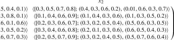
In many Turkey universities, doctoral dissertation will be reviewed by three experts anonymously and they have same importance in this review process. They will review dissertation according to five criteria, including topic selection and literature review, innovation, theory basis and special knowledge, capacity of scientific research and theses writing. Different weights are given to different criteria and the standards for those principles are as follows. After thorough investigation, four universities (alternatives) are taken into consideration, i.e., \(\{x_{1},x_{2},x_{3},x_{4}\}.\) There are many factors that affect the review process and five factors are considered based on the experience of the department personnel, including \(u_{1};\) topic selection and literature review (such as belonging to the leading edge of the subject or the hot research point has important theoretic significance and applied value; familiar with the research status and process for subject.), \(u_{2};\) innovation (such as have theoretical breakthrough; have positive influence and impact on the development of social economy and culture; creativity points, \(u_{3};\) theory basis and special knowledge (such as solid and broad theoretical foundation, also have specialized knowledge for the subject and related area) and \(u_{4};\) capacity of scientific research (such as independently scientific research ability; informative citing information; subject to be explored in depth) \(u_{5};\) theses writing(such as clear concept and logistics, smooth sentences, format specification, good school ethos) \(\cdot \) (whose weighted vector \(\omega =(0.1,0.3,0.2,0.3,0.1)\)) Our solution is to examine the university at different time intervals (four times a year: autumn, spring, winter, summer), which in turn gives rise to different membership functions for each university.
- Step 1 :
-
Construct the decision-making matrix \(A=({a}_{ij})_{m\times n}\) for decision as:

- Step 2 :
-
Applying the ITFMWG operator to derive the collective overall preference intuitionistic trapezoidal fuzzy multiset \({r}_{i}:\)
$$\begin{aligned} r_{1}= & {} \langle [0.16817,0.33178,0.48255,0.65678];\\&(0.27735,0.28378,0.40257,0.45370),\\&(0.96232,0.92592,0.97938,0.69384)\rangle ,\\ r_{2}= & {} \langle [0.24145,0.40568,0.64309,0.78228];\\&(0.28958,0.20773,0.45870,0.35515),\\&(0.93228,0.94370,0.92592,0.94945)\rangle ,\\ r_{3}= & {} \langle [0.20356,0.35958,0.53834,0.68854];\\&(0.59552,0.46395,0.19472,0.50804),\\&(0.95285,0.88175,0.88080,0.92949)\rangle ,\\ r_{4}= & {} \langle [0.13544,0.29438,0.44045,0.56567];\\&(0.44028,0.41406,0.50864,0.50801),\\&(0.96397,0.80973,0.81451,0.90565)\rangle . \end{aligned}$$ - Step 3 :
-
Calculate the distances between collective overall values \(r_{i}\) and intuitionistic trapezoidal fuzzy positive ideal solution \(r^{+}.\)
$$\begin{aligned} S(r_{1},r^{+})= & {} 0.29410,\\ S(r_{2},r^{+})= & {} 0.41407,\\ S(r_{3},r^{+})= & {} 0.34198,\\ S(r_{4},r^{+})= & {} 0.27944. \end{aligned}$$ - Step 4 :
-
Rank all the alternatives \(A_{i} (i=1,2,3,4)\) in accordance with the ascending order of \(S(r_{i},r^{+})\): \(A_{4}<A_{1}<A_{3}<A_{2},\) thus the most desirable alternative is \(A_{2}.\)
- Step 5 :
-
End


- Step 1 :
-
Construct the decision-making matrix \(A=({a}_{ij})_{m\times n},\) for decision as:


- Step 2 :
-
Applying the ITFMWA operator to derive the collective overall preference intuitionistic trapezoidal fuzzy multiset \({r}_{i}:\)
$$\begin{aligned} r_{1}= & {} \langle [0.71198,0.80871,0.86744,0.92073];\\&(0.79171,0.78605,0.83439,0.86489),\\&(0.77639,0.86405,0.81024,0.76144)\rangle ,\\ r_{2}= & {} \langle [0.76035,0.84044,0.91663,0.95280];\\&(0.78501,0.74213,0.85771,0.82793),\\&(0.74778,0.89425,0.82033,0.86320)\rangle ,\\ r_{3}= & {} \langle [0.74037,0.82344,0.88767,0.93018];\\&(0.90339,0.86156,0.74373,0.87462),\\&(0.70774,0.82936,0.81041,0.75288)\rangle ,\\ r_{4}= & {} \langle [0.70015,0.79739,0.85439,0.89614];\\&(0.086468,0.84804,0.87609,0.87864),\\&(0.66409,0.76757,0.78159,0.78288)\rangle . \end{aligned}$$ - Step 3 :
-
Calculate the distances between collective overall values \(r_{i}\) and intuitionistic trapezoidal fuzzy positive ideal solution \(r^{+}.\)
$$\begin{aligned} S(r_{1},r^{+})= & {} 0.535,\\ S(r_{2},r^{+})= & {} 0.55736,\\ S(r_{3},r^{+})= & {} 0.53694,\\ S(r_{4},r^{+})= & {} 0.54450. \end{aligned}$$ - Step 4 :
-
Rank all the alternatives \(A_{i} (i=1,2,3,4)\) in accordance with the ascending order of \(S(r_{i},r^{+})\): \(A_{1}<A_{3}<A_{4}<A_{2},\) thus the most desirable alternative is \(A_{2}.\)
- Step 5 :
-
End


Comparison analysis and discussion
To verify the feasibility and effectiveness of the proposed decision-making approach, a comparison analysis with TFM-numbers multi-criteria decision-making method, used by Ulucay et al. [49], is given, based on the same illustrative example. Clearly, the ranking order results are consistent with the result obtained in [49] (Table 1).
Conclusion
In this study, we have defined ITFM-numbers and operational laws, which are mainly based on t norm and t conorm. The ITFM-numbers are a generalization of trapezoidal fuzzy numbers, and intuitionistic trapezoidal fuzzy numbers which are commonly used in real decision problems with the lack of information or imprecision of the available information in real situations is more serious. So the research of ranking ITFM-numbers is very necessary and the ranking problem is more difficult than ranking ITFM-numbers due to additional multi-membership functions and multi-non-membership functions. So, some aggregation operators on ITFM-numbers by using algebraic sum and algebraic product is given in Definition 2.3. Based on the aggregation operators, we developed a multi-criteria making method, called ITFM-numbers multi-criteria decision-making method, by using the ITFMWG operator. Finally, we have proposed a practical example to discuss the applicability of ITFM-numbers multi-criteria decision-making method. In future work, we shall develop some new method and apply our theory to other fields, such as medical diagnosis, game theory, investment decision making, military system efficiency evaluation, and so on.
References
Atanassov KT (1999) Intuitionistic fuzzy sets. Pysica-Verlag A Springer-Verlag Company, New York
Uluçay V, Deli I, Şahin M (2016) Trapezoidal fuzzy multi-number and its application to multi-criteria decision-making problems. Neural Comput Appl. https://doi.org/10.1007/s00521-016-2760-3
De SK, Biswas R, Roy AR (2000) Some operations on intuitionistic fuzzy sets. Fuzzy Sets Syst 114(3):477–484
Kumar M (2014) Applying weakest t-norm based approximate intuitionistic fuzzy arithmetic operations on different types of intuitionistic fuzzy numbers to evaluate reliability of PCBA fault. Appl Soft Comput 23:387–406
Krohling RA, Pacheco AG, Siviero AL (2013) IF-TODIM: an intuitionistic fuzzy TODIM to multi-criteria decision making. Knowl Based Syst 53:142–146
Szmidt E, Kacprzyk J (2000) Distances between intuitionistic fuzzy sets. Fuzzy Sets Syst 114(3):505–518
Wang J, Zhang Z (2009) Multi-criteria decision-making method with incomplete certain information based on intuitionistic fuzzy number. Control Decis 24(2):226–230
Wu J, Huang HB, Cao QW (2013) Research on AHP with interval-valued intuitionistic fuzzy sets and its application in multi-criteria decision making problems. Appl Math Model 37(24):9898–9906
Xu Z (2012) Intuitionistic fuzzy multiattribute decision making: an interactive method. IEEE Trans Fuzzy Syst 20(3):514–525
Yu D (2014) Intuitionistic fuzzy information aggregation under confidence levels. Appl Soft Comput 19:147–160
Zhang Z (2012) A rough set approach to intuitionistic fuzzy soft set based decision making. Appl Math Model 36(10):4605–4633
Ban AI, Coroianu L (2012) Nearest interval, triangular and trapezoidal approximation of a fuzzy number preserving ambiguity. Int J Approx Reason 53(5):805–836
Chen S, Chang C (2016) Fuzzy multi attribute decision making based on transformation techniques of intuitionistic fuzzy values and intuitionistic fuzzy geometric averaging operators. Inf Sci Vol 352–353(20):133–149
Esmailzadeh M, Esmailzadeh M (2013) New distance between triangular intuitionistic fuzzy numbers. Adv Comput Math Appl 2(3):310–314
Kahraman C, Ghorabaee MK, Zavadskas EK, Onar SC, Yazdani M, Oztaysi B (2017) Intuitionistic fuzzy EDAS method: an application to solid waste disposal site selection. J Environ Eng Landsc Manag 25(1):1–12
Li DF, Nan JX, Zhang MJ (2010) A ranking method of triangular intuitionistic fuzzy numbers and application to decision making. Int J Comput Intell Syst 3(5):522–530
Li DF (2010) A ratio ranking method of triangular intuitionistic fuzzy numbers and its application to MADM problems. Comput Math Appl 60:1557–1570
Mondal SP, Roy TK (2015) System of differential equation with initial value as triangular intuitionistic fuzzy number and its application. Int J Appl Comput Math 1(3):449–474
Otay I, Oztaysi B, Onar SC, Kahraman C (2017) Multi-expert performance evaluation of healthcare institutions using an integrated intuitionistic fuzzy AHP–DEA methodology. Knowl Based Syst 133:90–106
Oztaysi B, Onar SC, Kahraman C, Yavuz M (2017) Multi-criteria alternative-fuel technology selection using interval-valued intuitionistic fuzzy sets. Transp Res Part D Transp Environ 53:128–148
Wang J, Nie R, Zhang H, Chen X (2013) New operators on triangular intuitionistic fuzzy numbers and their applications in system fault analysis. Inf Sci 251:79–95
Wan SP (2013) Power average operators of trapezoidal intuitionistic fuzzy numbers and application to multi-attribute group decision making. Appl Math Model 37:4112–4126
Zhinan H, Xu Z, Zhao H, Zhang R (2017) Novel intuitionistic fuzzy decision-making models in the framework of decision field theory. Information Fusion 33:57–70
Liu P, Liu Y (2014) An approach to multiple attribute group decision making based on intuitionistic trapezoidal fuzzy power generalized aggregation operator. Int J Comput Intell Syst 7(2):291–304
Wan SP, Dong JY (2015) Power geometric operators of trapezoidal intuitionistic fuzzy numbers and application to multi-attribute group decision making. Appl Soft Comput 29:153–168
Wu J, Cao QW (2013) Same families of geometric aggregation operators with intuitionistic trapezoidal fuzzy numbers. Appl Math Model 37(1):318–327
Ye J (2011) Expected value method for intuitionistic trapezoidal fuzzy multicriteria decision-making problems. Expert Syst Appl 38(9):11730–11734
Zhang X, Jin F, Liu P (2013) A grey relational projection method for multi-attribute decision making based on intuitionistic trapezoidal fuzzy number. Appl Math Model 37(5):3467–3477
Zhao S, Liang C, Zhang J (2015) Some intuitionistic trapezoidal fuzzy aggregation operators based on Einstein operations and their application in multiple attribute group decision making. Int J Mach Learn Cybern 8(2):547–569
Farhadinia B (2014) Sensitivity analysis in interval-valued trapezoidal fuzzy number linear programming problems. Appl Math Model 38(1):50–62
Li DF, Yang J (2015) A difference-index based ranking method of trapezoidal intuitionistic fuzzy numbers and application to multiattribute decision making. Math Comput Appl 20(1):25–38
Li X, Chen X (2015) Multi-criteria group decision making based on trapezoidal intuitionistic fuzzy information. Appl Soft Comput 30:454–461
Liu P, Jin F (2012) A multi-attribute group decision-making method based on weighted geometric aggregation operators of interval-valued trapezoidal fuzzy numbers. Appl Math Model 36(6):2498–2509
Farhadinia B, Ban AI (2013) Developing new similarity measures of generalized intuitionistic fuzzy numbers and generalized interval-valued fuzzy numbers from similarity measures of generalized fuzzy numbers. Math Comput Model 57:812–825
Deng G, Jiang Y, Fu J (2015) Monotonic similarity measures between intuitionistic fuzzy sets and their relationship with entropy and inclusion measure. Inf Sci 316:348–369
Liang X, Wei C (2014) An Atanassovs intuitionistic fuzzy multi-attribute group decision making method based on entropy and similarity measure. Int J Mach Learn Cybern 5(3):435–444
Shinoj TK, Sunil JJ (2013) Accuracy in collaborative robotics: an intuitionistic fuzzy multiset approach. Global J Sci Front Res Math Decis Sci 13(10):21–28
Yager RR (1986) on the theory of bags. Int J Gen Syst 13:23–37
Shinoj TK, John SJ (2012) Intuitionistic fuzzy multisets and its application in medical diagnosis. World Acad Sci Eng Technol 6(1):1418–1421
Shinoj TK, John SJ (2013) Intuitionistic fuzzy multisets. Int J Eng Sci Innov Technol (IJESIT) 2(6):1–24
Ibrahim AM, Ejegwa PA (2013) Some modal operators on intuitionistic fuzzy multisets. Int J Sci Eng Res 4(9):1814–1822
Ejegwa PA (2015) New operations on intuitionistic fuzzy multisets. J Math Inform 3:17–23
Rajarajeswari P, Uma N (2013) A study of normalized geometric and normalized hamming distance measures in intuitionistic fuzzy multi sets. Int J Sci Res 2:76–80
Ejegwa PA (2015) Mathematical techniques to transform intuitionistic fuzzy multisets to fuzzy sets. J Inf Comput Sci 10(2):169–172
Ejegwa PA, Awolola JA (2014) Intuitionistic fuzzy multiset (IFMS) in binomial distributions. Int J Sci Technol Res 3(4):335–337
Deepa C (2015) Some implication results related to intuitionistic fuzzy multisets. Int J Adv Res Comput Sci Softw Eng 5(4):361–365
Das S, Kar MB, Kar S (2013) Group multi-criteria decision making using intuitionistic multi-fuzzy sets. J Uncertain Anal Appl 10(1):1–16
Rajarajeswari P, Uma N (2013) On distance and similarity measures of intuitionistic fuzzy multi set. IOSR J Math 5(4):19–23
Rajarajeswari P, Uma N (2014) Correlation measure for intuitionistic fuzzy multi sets. Int J Res Eng Technol 3(1):611–617
Rajarajeswari P, Uma N (2014) Normalized hamming similarity measure for intuitionistic fuzzy multi sets and its application in medical diagnosis. Int J Math Trends Technol 5(3):219–225
Rajarajeswari P, Uma N (2013) Intuitionistic fuzzy multi similarity measure based on cotangent function. Int J Eng Res Technol 2(11):1323–1329 (ESRSA Publications)
Rajarajeswari P, Uma N (2014) Zhang and Fus similarity measure on intuitionistic fuzzy multi sets. Int J Innov Res Sci Eng Technol 3(5):12309–12317
Shinoj TK, John SJ (2015) Intuitionistic fuzzy multigroups. Ann Pure Appl Math 9(1):131–143
Ejegwa PA, Awolola JA (2013) Some algebraic structures of intuitionistic fuzzy multisets (IFMSs). Int J Sci Technol 2(5):373–376
Shinoj TK, John SJ (2015) Topological structures on intuitionistic fuzzy multisets. Int J Sci Eng Res 6(3):192–200
Zadeh LA (1965) Fuzzy sets. Inf Control 8:338–353
Zimmermann H-J (1993) Fuzzy set theory and its applications. Kluwer Academic Publishers, Dordrecht
Sebastian S, Ramakrishnan TV (2010) Multi-fuzzy sets. Int Math Forum 5(50):2471–2476
Wei SH, Chen SM (2006) A new similarity measure between generalized fuzzy numbers. In: SCIS, ISIS, vol 2006. Japan Society for Fuzzy Theory and Intelligent Informatics, Tokyo Institute of Technology, Tokyo, Japan, 20–24 September 2006, pp 315–320
Author information
Authors and Affiliations
Additional information
Publisher's Note
Springer Nature remains neutral with regard to jurisdictional claims in published maps and institutional affiliations.
Rights and permissions
Open Access This article is distributed under the terms of the Creative Commons Attribution 4.0 International License (http://creativecommons.org/licenses/by/4.0/), which permits unrestricted use, distribution, and reproduction in any medium, provided you give appropriate credit to the original author(s) and the source, provide a link to the Creative Commons license, and indicate if changes were made.
About this article

Cite this article
Uluçay, V., Deli, I. & Şahin, M. Intuitionistic trapezoidal fuzzy multi-numbers and its application to multi-criteria decision-making problems. Complex Intell. Syst. 5, 65–78 (2019). https://doi.org/10.1007/s40747-018-0074-z
Received:
Accepted:
Published:
Issue Date:
DOI: https://doi.org/10.1007/s40747-018-0074-z