
Abstract
We prove a regularity result for minimal configurations of variational problems involving both bulk and surface energies in some bounded open region \(\varOmega \subseteq {\mathbb {R}}^n\). We will deal with the energy functional \({\mathscr {F}}(v,E):=\int _\varOmega [F(\nabla v)+1_E G(\nabla v)+f_E(x,v)]\,dx+P(E,\varOmega )\). The bulk energy depends on a function v and its gradient \(\nabla v\). It consists in two strongly quasi-convex functions F and G, which have polinomial p-growth and are linked with their p-recession functions by a proximity condition, and a function \(f_E\), whose absolute valuesatisfies a q-growth condition from above. The surface penalization term is proportional to the perimeter of a subset E in \(\varOmega \). The term \(f_E\) is allowed to be negative, but an additional condition on the growth from below is needed to prove the existence of a minimal configuration of the problem associated with \({\mathscr {F}}\). The same condition turns out to be crucial in the proof of the regularity result as well. If (u, A) is a minimal configuration, we prove that u is locally Hölder continuous and A is equivalent to an open set \({\tilde{A}}\). We finally get \(P(A,\varOmega )={\mathscr {H}}^{n-1}(\partial {\tilde{A}}\cap \varOmega \)).
1 Introduction and statement
The problem of finding the minimal energy configuration of a mixture of two materials in a bounded open set \(\varOmega \subseteq {\mathbb {R}}^n\), penalized by the perimeter of the contact interface between the two materials, has been fully examined in mathematical literature (see for example [2, 3, 6, 8, 10, 15, 17,18,19,20]).
Let \(p>1\) and define \({\mathscr {A}}(\varOmega )\) as the set of all subsets of \(\varOmega \) with finite perimeter.Consider \(F,G\in C^1({\mathbb {R}}^n)\) and define \(f_E:=g+1_E h\), where \(E\in {\mathscr {A}}(\varOmega )\) and \(g,h:\varOmega \times {\mathbb {R}}\rightarrow {\mathbb {R}}\) are two Borel measurable and lower semicontinuous functions with respect to the real variable. We will deal with the following energy functional:
where \((v,E)\in \big (u_0+ W^{1,p}_0 (\varOmega )\big )\times {\mathscr {A}}(\varOmega )\), with \(u_0\in W^{1,p}(\varOmega )\). The regularity of minimizers (u, A) of the functional \({\mathscr {F}}\) was recently investigated in [6, 9, 10] for the constrained problem where the volume of the region A in \(\varOmega \) is prescribed but the forcing term \(f_A\) is zero. In the quadratic case \(p=2\) Ambrosio and Buttazzo [3] proved the regularity for minimizers of \({\mathscr {F}}\) in the case that \(f_A\) is not zero. We are going to extend this result to functionals with polinomial growth.
We assume that there exist some positive constants \(l,L,\alpha ,\beta \) and \(\mu \ge 0\) such that
-
F and G have p-growth:
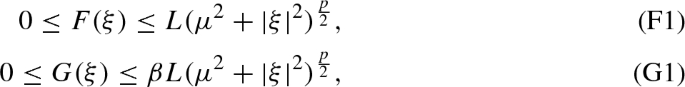
for all \(\xi \in {\mathbb {R}}^n\).
-
F and G are strongly quasi-convex:
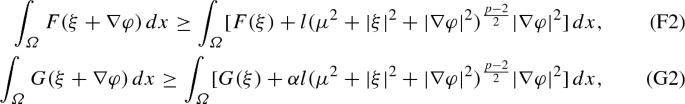
for all \(\xi \in {\mathbb {R}}^n\) and \(\varphi \in C^1_c(\varOmega )\).
-
there exist two positive constants \(t_0\), a and \(0<m<p\) such that for every \(t>t_0\) and \(\xi \in {\mathbb {R}}^n\) with \(|\xi |=1\), it holds
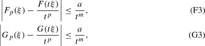
where \(F_p\) and \(G_p\) are the p-recession functions of F and G (see Definition 2.1).


We remark that the proximity conditions (F3) and (G3) are trivially satisfied if F and G are positively p-homogeneous.
The first of the following assumptions on g and h is essential to prove the existence of a minimal configuration. The same condition turns out to be crucial in the proof of the regularity result as well. We assume that there exist a function \(\gamma \in L^1(\varOmega )\) and two constants \(C_0>0\) and \(k\in {\mathbb {R}}\), with \(k<\frac{l}{2^{p-1}\lambda }\), being \(\lambda =\lambda (\varOmega )\) the first eigenvalue of the p-Laplacian on \(\varOmega \) with boundary datum \(u_0\), such that
-
g and h satisfy the following assumptions:
$$\begin{aligned} g(x,s)\ge \gamma (x)-k|s|^p, \quad h(x,s)\ge \gamma (x)-k|s|^p, \end{aligned}$$(1.1)for almost all \((x,s)\in \varOmega \times {\mathbb {R}}\).
-
g and h satisfy the following growth conditions:
$$\begin{aligned} |g(x,s)|\le C_0(1+|s|^q),\quad |h(x,s)|\le C_0(1+|s|^q), \end{aligned}$$(1.2)for all \((x,s)\in \varOmega \times {\mathbb {R}}\), with the exponent
$$\begin{aligned} q\in {\left\{ \begin{array}{ll} {[}p,+\infty ) &{}\text {if }n=2,\\ {[}p,p^*) &{}\text {if }n>2 \end{array}\right. } \end{aligned}$$fixed.
We want to study the following problem:

The main result of the paper is the following theorem about the regularity of solutions of problem P.
Theorem 1.1
Let (u, A) be a solution of (P). Then
-
1.
u is locally Hölder continuous.
-
2.
A is equivalent to an open set \({\tilde{A}}\), that is
$$\begin{aligned} {\mathscr {L}}^n(A\Delta {\tilde{A}})=0 \quad \text {and}\quad P(A,\varOmega )=P({\tilde{A}},\varOmega )={\mathscr {H}}^{n-1}(\partial {\tilde{A}}\cap \varOmega ). \end{aligned}$$
The idea of its proof is similar to that of Theorem 2.2 in [3], which in turns relies on the ideas introduced in [7]. The regularity of u is proved in Theorem 4.1 and the regularity of A follows from Proposition 5.1. The proof will be discussed in the final section.
The same arguments can be used to treat also the volume-constraint problem

for some \(0<d<{\mathscr {L}}^n(\varOmega )\). The following theorem holds true.
Theorem 1.2
There exists \(\lambda _0>0\) such that if (u, A) is a minimizer of the functional
for some \(\lambda \ge \lambda _0\) and among all configurations (v, E) such that \(v\in u_0+W^{1,p}_0(\varOmega )\) and \(E\in {\mathscr {A}}(\varOmega )\), then \({\mathscr {L}}^n(A)=d\) and (u, A) is a minimizer of problem (Q) . Conversely, if (u, A) is a minimizer of the problem (Q), then it is a minimizer of \({\mathscr {F}}_{\lambda }\), for all \(\lambda \ge \lambda _0\).
The proof of the previous theorem is a straightforward adaptation of the proof of Theorem 1.4 in [6]. The term concerning the function \(f_E\) can be treated as a constant, thanks to the boundedness stated in Theorem 4.1. We finally remark that the term \(\lambda |{\mathscr {L}}^n(E)-d|\) in the functional \({\mathscr {F}}_\lambda \) can be inglobed in \(f_E\), since it is bounded. For this reason, Theorem 1.1 is still valid also for minimal configurations of \({\mathscr {F}}_\lambda \) and, consequently, for solutions of problem (Q).
2 Notation and preliminary results
Throughout the paper we denote by \(\langle \cdot ,\cdot \rangle \) and \(\left\Vert \cdot \right\Vert \) respectively the Euclidean inner product in \({\mathbb {R}}^n\) and the associated norm. We write \({\mathscr {L}}^n\) for the Lebesgue measure. Furthermore, we denote by \(B_r(x)\) the ball centered in \(x\in {\mathbb {R}}^n\) with radius \(r>0\) (if \(x=0\), we write simply \(B_r\)), by \(\omega _n\) the measure of \(B_1\), and with \(Q_r(x)\) the cube centered in \(x\in {\mathbb {R}}^n\) with side \(r>0\). We write the symbols \(\rightharpoonup \) and \(\rightarrow \) referring to weak and strong convergence, respectively.
We often denote by c a general constant that could vary from line to line, even within the same line of estimates. Relevant dependencies on parameters and special constants will be suitably emphasized using brackets.
Throughout this section we denote with H a function belonging to \(C^1({\mathbb {R}}^n)\) and satisfying for some positive constants \({\tilde{l}}\) and \({\tilde{L}}\) the same kind of assumptions imposed on F and G:
for all \(\xi \in {\mathbb {R}}^n\) and \(\varphi \in C^1_c(\varOmega )\). We collect some definitions and well-known results that will be used later. We start giving the definition of p-recession function of H.
Definition 2.1
The p-recession function of H is defined by
for all \(\xi \in {\mathbb {R}}^n\).
Remark 2.2
It’s clear that \(H_p\) is positively p-homogeneous, which means that
for all \(\xi \in {\mathbb {R}}^n\) and \(s>0\). It’s also true that the growth condition of H implies the following growth condition of \(H_p\):
for any \(\xi \in {\mathbb {R}}^n\).
Next lemma establishes strong quasi-convexity of \(H_p\), provided H verifies an appropriate growth condition. Its proof is in [12] (Lemma 2.8).
Lemma 2.3
Let H as above. If there exist two positive constants \({\tilde{t}}_0\), \({\tilde{d}}\) and \(0<{\tilde{m}}<p\) such that for every \(t>{\tilde{t}}_0\) and \(\xi \in {\mathbb {R}}^n\) with \(|\xi |=1\), it holds
then
for all \(\xi \in {\mathbb {R}}^n\) and \(\varphi \in C^1_c(\varOmega )\).
Let’s recall some other useful lemmas.
Lemma 2.4
Let H be as above. It holds that
for all \(\xi \in {\mathbb {R}}^n\).
Lemma 2.5
Let H as above. There exists a positive constant \({\tilde{c}}={\tilde{c}}(p,{\tilde{l}},{\tilde{L}},\mu )\) such that
for all \(\xi \in {\mathbb {R}}^n\).
The proof of Lemma 2.4 can be found in [14] (Lemma 5.2), while Lemma 2.5 is proved in [6] (Lemma 2.3). We define the auxiliary function
for all \(\xi \in {\mathbb {R}}^n\).
Next Lemma has been proved in [13] (Lemma 2.1) for \(p\ge 2\) and in [1] (Lemma 2.1) for \(1<p<2\).
Lemma 2.6
There exists a constant \(c=c(n,p)\) such that
for all \(\xi ,\eta \in {\mathbb {R}}^n\).
Lemma 2.7
Let \(\lbrace u_h \rbrace _{h\in {\mathbb {N}}}\subseteq W^{1,p}(B_1)\) and \(u\in W^{1,p}(B_1)\) such that \(u_h\rightharpoonup u\) in \(W^{1,p}(B_1)\). Assume that \(\lbrace \nabla u_h\rbrace _{h\in {\mathbb {N}}}\) is bounded in \(L^p(B_1)\). If
then \(u_h \rightarrow u\) in \(W^{1,p}_{loc}(B_1)\).
The proof of the previous lemma follows from Lemma 2.6. If \(p\ge 2\) the hypothesis ofboundedness of \(\lbrace \nabla u_h\rbrace _{h\in {\mathbb {N}}}\) is superfluous. If \(1<p<2\), by Hölder inequality we gain the stated result.
The following theorem has been proved in [12] (Theorem 2.2).
Theorem 2.8
Let H be as above and let \(v\in W^{1,p}(\varOmega )\) be a local minimizer of the functional
where \(w\in v+W^{1,p}_0(\varOmega )\). Then v is locally Lipschitz-continuous in \(\varOmega \) and there exists a constant \(c= c(n,p,{\tilde{l}},{\tilde{L}})>0\) such that
for all \(B_R(x_0)\subseteq \varOmega \).
Corollary 2.9
Let \({\mathscr {H}}\) and \(v\in W^{1,p}(\varOmega )\) be as in Theorem 2.8. Then there exists a constant \(c_{{\mathscr {H}}}=c_{{\mathscr {H}}}(n,p,{\tilde{l}},{\tilde{L}})>0\) such that
for all \(B_R(x_0)\subseteq \varOmega \) and \(0<r<R\).
3 Existence of minimizing couples
Theorem 3.1
The minimum problem (P) admits at least a solution.
Proof
We initially remark that problem (P) can be written as follows:
where
Since F, G are strongly quasi-convex and g, h are lower semicontinuous in the real variable s, the functional \({\mathscr {F}}\) is lower semicontinuous with respect to the weak convergence of \(\nabla v_h\) in \(L^p\) and the strong converge of \(v_h\) in \(L^p\) (see [5] or [16]). Moreover, the coerciveness of
is granted by Lemma 2.5. Therefore the minimum problem (3.2) admits a solution. Let \(\lbrace A_h \rbrace _{h\in {\mathbb {N}}}\subseteq {\mathscr {A}}(\varOmega )\) be a minimizing sequence for problem (3.1). It follows that the sequence \(\lbrace P(A_h,\varOmega ) \rbrace _{h\in {\mathbb {N}}}\) is bounded and so, by compactness, there exists \(A\in {\mathscr {A}}(\varOmega )\) such that \(1_{A_h}\rightarrow 1_A\) in \(L^1_{loc}(\varOmega )\). Let \(u_h\in u_0+W^{1,p}_0(\varOmega )\) a solution of problem (3.2) associated with \(A_h\), for all \(h\in {\mathbb {N}}\). The sequence \(\lbrace u_h \rbrace _{h\in {\mathbb {N}}}\) is bounded in \(W^{1,p}(\varOmega )\); indeed, by (1.1) and Poincaré inequality we obtain
Hence, we can extract a subsequence (not relabelled) such that \(u_h\rightharpoonup u\) in \(W^{1,p}(\varOmega )\). By definition of minimum we infer
Applying again Ioffe lower semicontinuity result (see for instance [16] or [4], Theorem 5.8) to the integrand
where \(x\in \varOmega \), \(s_1\in [0,1]\), \(s_2\in {\mathbb {R}}\) and \(\xi \in {\mathbb {R}}^n\), we obtain
Therefore, by the lower semicontinuity of perimeter we finally gain
which proves that A is a minimizer of problem (3.1) and so (u, A) is a minimizing couple of problem (P). \(\square \)
4 Higher integrability and Hölder continuity of minimizers
The following theorem shows that local minimizers of the functional \({\mathscr {F}}(\cdot ,E)\), with \(E\in {\mathscr {A}}(\varOmega )\) fixed, are Hölder continuous and a higher integrability property for the gradient holds true. The proof of this result is standard and can be carried on adopting the obvious adaptation in the proof of Theorem 3.1 in [3].
Theorem 4.1
Let (u, A) be a solution of (P). Then the following facts hold:
-
u is locally bounded in \(\varOmega \) by a constant depending only on \(n,p,q,\alpha ,\beta ,l,L, \mu ,C_0,\left\Vert u\right\Vert _{L^p(\varOmega )}\) and is locally Hölder continuous in \(\varOmega \).
-
Let \(\varOmega _0\Subset \varOmega \), \(\tau =\text {dist}(\varOmega _0,\partial \varOmega )\) and \(K=\lbrace x\in \varOmega \,:\, \text {dist}(x,\varOmega _0)\le \frac{\tau }{2} \rbrace \). Then there exist two constants \(\gamma >0\) and \(r>p\) depending only on \(n,p,q,\beta ,l,L,\mu ,C_0,\left\Vert u\right\Vert _{L^\infty (K)}\) such that
$$\begin{aligned} \int _{Q_{\frac{R}{2}}(y)}|\nabla u|^r\,dx\le \gamma \bigg [ R^{n\big ( 1-\frac{r}{p}\big )}\bigg ( \int _{Q_R(y)}|\nabla u|^p\,dx \bigg )^{\frac{r}{p}} +R^n \bigg ], \end{aligned}$$for all \(y\in \varOmega _0\) and \(Q_R(y)\subseteq K\).
5 Regularity of the set
The following proposition is the main result of this section and also the main ingredient to prove Theorem 1.1.
Proposition 5.1
Let (u, A) be a solution of (P). Then for every compact set \(K\subseteq \varOmega \) there exists a constant \(\xi \in (0,\text {dist}(K,\partial \varOmega ))\) such that if \(y\in K\) and for some \(\rho <\xi \) it holds
then
The proof of the previous proposition relies on Proposition 5.5, which is an iteration of the decay estimate in Theorem 5.4. The following definition is crucial in the rescaling argument used in the proof of Theorem 5.4 (see (5.11)).
Definition 5.2
(Asymptotically minimizing sequence) Let \(\lbrace (u_h,A_h) \rbrace _{h\in {\mathbb {N}}}\subseteq W^{1,p}(B_1)\times {\mathscr {A}}(B_1)\) and \(\lbrace \lambda _h \rbrace _{h\in {\mathbb {N}}}\subseteq {\mathbb {R}}^+\). We say that the sequence \(\lbrace (u_h,A_h) \rbrace _{h\in {\mathbb {N}}}\) is \(\lambda _h\)-asymptotically minimizing if and only if for any compact set \(K\subseteq B_1\) and any couple \(\lbrace (u'_h,A'_h) \rbrace \subseteq W^{1,p}(B_1)\times {\mathscr {A}}(B_1)\) formed by a bounded sequence \(\lbrace u'_h\rbrace _{n\in {\mathbb {N}}}\) in \(W^{1,p}(B_1)\) with \(\text {spt}(u_h-u'_h)\subseteq K\) and a sequence of sets \(\lbrace A'_h\rbrace _{n\in {\mathbb {N}}}\) with \(A_h\Delta A'_h\subseteq K\), we have
where \(\lbrace \eta _h \rbrace _{h\in {\mathbb {N}}}\subseteq {\mathbb {R}}\) is an infinitesimal sequence.
In the proof of Theorem 5.4 we will show that the sequence of appropriately rescaled minimal configurations of problem (P) is asymptotically minimizing. The following theorem is concerned with the behaviour of asymptotically minimizing sequences.
Theorem 5.3
Let \(\lbrace \lambda _h \rbrace _{h\in {\mathbb {N}}}\subseteq {\mathbb {R}}^+\) and \(\lbrace (u_h,A_h) \rbrace _{h\in {\mathbb {N}}}\subseteq W^{1,p}(B_1)\times {\mathscr {A}}(B_1)\). Assume that \((u_h,A_h)\) is \(\lambda _h\)-asymptotically minimizing and that
-
(i)
\(\left\{ {\int _{B_1}}[F_p(\nabla u_h)+1_{A_h}G_p(\nabla u_h)]\,dy+\lambda _h P(A_h,B_1) \right\} _{h\in {\mathbb {N}}}\) is bounded.
-
(ii)
\(u_h \rightharpoonup u\) in \(W^{1,p}(B_1)\).
-
(iii)
\(1_{A_h} \rightarrow 1_A\) in \(L^1(B_1)\) and \(\lambda _h\rightarrow +\infty \).
-
(iv)
\(G_p(\nabla u_h)\) is locally equi-integrable in \(B_1\).
Then
-
(a)
\(u_h \rightarrow u\) in \(W^{1,p}_{loc}(B_1)\).
-
(b)
\(\lambda _h P(A_h,B_\rho )\rightarrow 0\), for all \(\rho \in (0,1)\).
-
(c)
\(A=\emptyset \) or \(A=B_1\) and u minimizes the functional \( \int _{B_1}[F_p(\nabla v)+1_A G_p(\nabla v)]\,dy\) among all \(v\in u+W^{1,p}_0(B_1)\).
Proof
Let’s prove (a). The hypothesis (iv) implies that
Let \({\tilde{u}}_h:=(1-\psi )u_h+\psi u\), \(\psi \in C^{\infty }_c(B_1)\), with \(0\le \psi \le 1\). Then \(\nabla {\tilde{u}}_h=(u-u_h)\nabla \psi +(1-\psi )\nabla u_h+\psi \nabla u\). Testing \((A_h,{\tilde{u}}_h)\), we have
where \(\lbrace \eta _h \rbrace _{h\in {\mathbb {N}}}\subseteq {\mathbb {R}}\) is the infinitesimal sequence in (5.1). By the convexity of \(F_p\) and \(G_p\) and Lemma 2.4, it follows that
Using the previous one in (5.3), we obtain
The second term in the right hand side is infinitesimal; indeed, using the Hölder inequality, we have
which tends to 0 as h approaches \(+\infty \). So we can inglobe the second term in the right hand side of (5.4) in \(\eta _h\). Add \(\displaystyle {\int _{B_1}}\psi 1_A G_p(\nabla u_h)\,dy\) to both sides in (5.4) in order to obtain
where \(\lbrace {\tilde{\eta }}_h \rbrace _{h\in {\mathbb {N}}}\subseteq {\mathbb {R}}\) is infinitesimal. Thanks to (5.2), we can pass to the upper limit and obtain
Finally, by lower semicontinuity, we gain
By the strong quasi-convexity of \(F_p\) and \(G_p\) and Lemma 2.6, we have
Let \(h\rightarrow +\infty \) in (5.6). By the ii) and (5.5), we infer
Thanks to Lemma 2.7 and the arbitrariety of \(\psi \), we conclude that \(u_h \rightarrow u\) in \(W^{1,p}_{loc}(B_1)\).
Let’s prove b). Since \(\lambda _h\rightarrow +\infty \) and the energies are bounded by an appropriate constant c, it holds that
Let \(h\rightarrow +\infty \) in the previous inequality. By semicontinuity we infer that \(P(A,B_1)=0\). Thanks to isoperimetric inequality it follows that \(A=\emptyset \) or \(A=B\). We’ll discuss the case \(A=\emptyset \), being the other one similar. For h large enough, by the isoperimetric inequality we have
Denoting \(1_h(\rho )=1_{A_h\cap \partial B_\rho }\), for all \(h\in {\mathbb {N}}\) and \(\rho \in (0,1)\), the coarea formula provides that
which means that the sequence of functions \(\bigg \lbrace \lambda _h\int _{\partial B_\rho }1_h(\rho )\,d{\mathscr {H}}^{n-1} \bigg \rbrace _{h\in {\mathbb {N}}}\) converges to 0 in \(L^1(0,1)\). Thus, it converges to 0 for almost every \(\rho \in (0,1)\). Then, for every \(\rho \in (0,1)\) fixed, we can find a sequence \(\lbrace \rho _h\rbrace _{h\in {\mathbb {N}}}\subseteq \big ( \rho ,\frac{1+\rho }{2} \big )\) such that
as h approaches \(+\infty \). Comparing \(\lbrace (u_h,A_h)\rbrace _{h\in {\mathbb {N}}}\) and \(\lbrace (u_h,A_h\setminus {\overline{B}}_{\rho _h})\rbrace _{h\in {\mathbb {N}}}\) , using (5.7) and the equality
there exists an infinitesimal sequence \(\lbrace \eta _h \rbrace _{h\in {\mathbb {N}}}\subseteq {\mathbb {R}}\) such that
provided h is so large that \(A_h\subseteq {\overline{B}}_{\frac{\rho +1}{2}}\). Thus, thanks to (5.7) the sequence \(\lbrace \lambda _h P(A_h,B_{\rho _h}) \rbrace _{h\in {\mathbb {N}}}\) is infinitesimal and we can conclude that
as h approaches \(+\infty \), since \(\rho _h>\rho \).
Let’s prove c). Comparing \((A_h,u_h)\) with \((A_h,{\tilde{u}}_h)=(A_h,u_h+\varphi )\), where \(\varphi \in C^1(B_1)\) and supp(\(\varphi \))\(\subseteq B_{\rho }\), we have
with \(\lbrace \eta _h\rbrace _{h\in {\mathbb {N}}}\subseteq {\mathbb {R}}\) infinitesimal and \(\rho \in (0,1)\) arbitrary. Thanks to a), we can use the dominated convergence theorem in order to pass to the limit as h approaches \(+\infty \), obtaining
By the arbitrariety of \(\rho \) and \(\varphi \) we can conclude the proof. \(\square \)
The following theorem is the main tool for proving Proposition 5.1.
Theorem 5.4
(Energy decay estimate) Let \(K\subseteq \varOmega \) be a compact set, \(\delta =\text {dist}(K,\partial \varOmega )>0\) and \(\varepsilon \in (0,1)\). Let \({\tilde{c}}={\tilde{c}}(p,l,L,\alpha ,\beta ,\mu )\) and \(c_{{\mathscr {H}}}=c_{{\mathscr {H}}}(n,p,l,L,\alpha ,\beta )\) the constants of Lemma 2.5 and Corollary 2.9 for
Moreover, let \(\tau \in (0,1)\) such that \(\tau ^\varepsilon <\frac{1}{2(1+\omega _n{\tilde{c}})}\). Then there exist two positive constants \(\gamma \) and \(\theta \) such that for any solution (u, A) of the problem (P) and for any ball \(B_\rho (y)\) with \(y\in K\) and \(\rho \in (0,\frac{\delta }{2})\) the two estimates
imply that
Proof
Let’s suppose by contradiction that there exist two sequences \(\lbrace \gamma _h\rbrace _{h\in {\mathbb {N}}}\) and \(\lbrace \theta _h \rbrace _{h\in {\mathbb {N}}}\) which tend to 0, a sequence of minimizing couples \(\lbrace (w_h,D_h) \rbrace _{h\in {\mathbb {N}}}\) of (P) and a sequence of balls \(\lbrace B_{\rho _h}(x_h)\rbrace _{h\in {\mathbb {N}}}\), with \(x_h\in K\) and \(\rho _h\in (0,\frac{\delta }{2})\), for all \(h\in {\mathbb {N}}\), such that these estimates hold:
In what follows it will be important that the sequence \(\lbrace w_h \rbrace _{h\in {\mathbb {N}}}\) is locally equibounded in \(\varOmega \). It descends from Theorem 4.1 once we have proved that \(\lbrace w_h \rbrace _{h\in {\mathbb {N}}}\) is bounded in \(W^{1,p}(\varOmega )\), which holds true; indeed, by the minimality of \((w_h,D_h)\), (F1), (1.1) and Poincaré inequality it follows that
since \(k<\frac{l}{2^{p-1}\lambda }\). Rescale the functions \(w_h\); define
where \({\overline{w}}_h=\fint _{B_1}w_h(x_h+\rho _hy)\,dy\), for all \(h\in {\mathbb {N}}\). By the usual change of variables \(x:=x_h+\rho _h y\), we have:
Rescale the estimates (5.8), (5.9) and (5.10), obtaining
We want to apply Theorem 5.3 to the sequence \(\lbrace (u_h,A_h) \rbrace _{n\in {\mathbb {N}}}\).
Firstly, let’s prove that \(\lbrace (u_h,A_h) \rbrace _{n\in {\mathbb {N}}}\) is \(\lambda _h\)-asymptotically minimizing. Let \(K'\subseteq B_1\) be a compact set and \(\lbrace (u'_h,A'_h) \rbrace _{h\in {\mathbb {N}}}\) such that \(\lbrace u'_h \rbrace _{h\in {\mathbb {N}}}\) is a bounded sequence in \(W^{1,p}(B_1)\) with spt(\(u'_h-u_h\))\(\subseteq K'\) and \(A'_h\subseteq B_1\) with \(A'_h\Delta A_h\subseteq K'\).
Rescale the functions \(u'_h\):
Compare the two sequences \(\lbrace (w_h,D_h) \rbrace _{h\in {\mathbb {N}}}\) and \(\lbrace (w'_h,D'_h) \rbrace _{h\in {\mathbb {N}}}\): by the minimality of \(\lbrace (w_h,D_h) \rbrace _{h\in {\mathbb {N}}}\) and by (1.2) we have
In the sixth line of the previous inequality we need \(F_p\) and \(G_p\) in place of F and G, so by (F3) and (G3) we infer
Thus by homogeneity, (F3) and (G3) we get
In order to prove that \(\lbrace (u_h,A_h)\rbrace _{h\in {\mathbb {N}}}\) is \(\lambda _h\)-asymptotically minimizing, we need to show that
By (5.13) it’s clear that \(\lim \nolimits _{h\rightarrow +\infty }\frac{\rho _h}{\gamma _h}=0\). Since \(\lbrace w_h \rbrace _{n\in {\mathbb {N}}}\) is locally equibounded in \(\varOmega \), also \(\lim \nolimits _{h\rightarrow +\infty }\frac{1}{\gamma _h\rho _h^{n-1}}\int _{B_{\rho _h}(x_h)}|w_h|^q\,dx=0\). It remains to prove that
Let’s prove (5.15). Since \(\lbrace w_h \rbrace _{h\in {\mathbb {N}}}\) is locally equibounded by a constant \(M>0\), substituting the expression of \({\overline{w}}_h\) from (5.11) it follows that
where we used the Sobolev embedding theorem. Since \(q\ge p\), \(\lbrace u'_h \rbrace _{h\in {\mathbb {N}}}\) and \(\lbrace u_h \rbrace _{h\in {\mathbb {N}}}\) are bounded in \(W^{1,p}(B_1)\) and \(\lim \nolimits _{h\rightarrow +\infty }\displaystyle \frac{\rho _h}{\gamma _h}=0\), we conclude that (5.15) holds true. We are left to prove (5.16). By Hölder inequality we get
Since \(\lim \nolimits _{h\rightarrow +\infty }\displaystyle \frac{\rho _h}{\gamma _h}=0\) and \(\lbrace u'_h \rbrace _{h\in {\mathbb {N}}}\), \(\lbrace u_h \rbrace _{h\in {\mathbb {N}}}\) are bounded in \(W^{1,p}(B_1)\), we obtain (5.16).
Thanks to (5.12) there exist a function \(u\in W^{1,p}(B_1)\) and a set of finite perimeter \(A\subseteq B_1\) such that
We are finally in position to apply Theorem 5.3 to \(\lbrace (u_h,A_h)\rbrace _{h\in {\mathbb {N}}}\). It remains only to prove that \(G_p(\nabla u_h)\) is locally equi-integrable, which we will prove later. As a consequence of Theorem 5.3 we have that \(A=\emptyset \) or \(A=B_1\). We’ll discuss the case \(A=\emptyset \), being the other one similar. Thanks to Corollary 2.9 and Lemma 2.5, by lower semicontinuity we infer
Using inequality (5.12), (5.14) and the (b) of Theorem 5.3, we gain
Comparing the previous estimate with (5.17) we reach a contradiction.
We are only left to prove the equi-integrability of \(G_p(\nabla u_h)\) in \(B_1\). It’s enough to prove that for all \(t\in (0,1)\) there exists \(r>p\) such that
Indeed, fix \(\varepsilon >0\), a compact set \(K'\subseteq B_1\) and \(A\subseteq K'\). Then by the growth condition of \(G_p\) and the Hölder inequality, it follows that
In order to prove (5.18), we can apply Theorem 4.1: there exist two constants \(\gamma >0\) and \(r>p\) depending only on \(n,p,q,\beta ,l,L,\mu ,C_0,\left\Vert w_h\right\Vert _{L^\infty (K)}\) such that for all \(h\in {\mathbb {N}}\) and \(y\in K\), with dist(\(Q_{2\rho _h}(y),K\))\(\le \frac{\delta }{2}\) we have the following local higher summability:
It can be also shown that the dependence of \(\gamma \) and r on \(\left\Vert w_h\right\Vert _{L^\infty (K)}\) is uniform with respect to h, since \(\lbrace w_h \rbrace _{h\in {\mathbb {N}}}\) is locally equibounded in \(\varOmega \).
Fix \(t\in (0,1)\). By a covering argument it follows that
Rescale and write the estimate in terms of \(u_h\):
where \(M'>0\) is an upper bound for \(\lbrace \left\Vert u_h\right\Vert _{W^{1,p}(\varOmega )}\rbrace _{h\in {\mathbb {N}}}\). Using (5.13) we prove our assertion. \(\square \)
The last proposition that we need to prove Proposition 5.1 follows from the previous result and is based on an iteration argument.
Proposition 5.5
Let \(K,\gamma ,\theta ,\delta \) be given by Theorem 5.4 and let (u, A) be a solution of (P). Let \(y\in K\) and denote
Moreover, let \(\varepsilon \in (0,1)\) and \(\sigma \in (n-1,n-\varepsilon )\) such that there exists \(\tau \in (0,1)\) satisfying \(\displaystyle {\frac{c_{{\mathscr {H}}}(1+\beta )L}{l}\tau ^{n-\varepsilon }<\tau ^\sigma }\) and \(\tau ^\varepsilon <\frac{1}{2(1+\omega _n{\tilde{c}})}\). Set \(\xi =\min \lbrace \text {dist}(y,\partial \varOmega ),\gamma ,\tau ^{\sigma }\gamma \theta \rbrace \). If\(\Psi (\rho )<\xi \rho ^{n-1}\) for some \(\rho \in (0,\xi )\), then
In particular,
Proof
Let’s assume that \(\Psi (\rho )<\xi \rho ^{n-1}\) for some \(\rho \in (0,\xi )\). Since \(\Psi \) is nondecreasing, it suffices to show by induction on \(j\in {\mathbb {N}}_0\) that
where \(\eta _j=\tau ^j\rho \). Since we chose \(\xi <\gamma \), the inequality holds true if \(j=0\). Let’s assume that it holds true for \(j>0\). By induction we state
that is \(\Psi (\eta _j)<\gamma \eta _j^{n-1}\). If \(\theta \Psi (\eta _j)>\eta _j^n\), thanks to the choice \(\xi <\text {dist}(y,\partial \varOmega )\), we can apply Theorem 5.4 and the inductive hypothesis in order to obtain
If \(\theta \Psi (\eta _j)\le \eta _j^n\), then we can state
Indeed
since \(\xi <\tau ^{\sigma }\gamma \theta \). Finally, using that \(\Psi \) is non-decreasing, we have
which concludes the proof. \(\square \)
Finally, we can prove Proposition 5.1 choosing \(\xi =\min \lbrace \text {dist}(K,\partial \varOmega ),\gamma ,\tau ^{\sigma }\gamma \theta \rbrace \), where\(\gamma ,\tau ,\sigma ,\theta \) are given by Proposition 5.5.
6 Proof of the main theorem
In this section we give the proof of Theorem 1.1, which makes use of the results we obtained in the previous sections.
Proof
(of Theorem 1.1) The assertion 1. follows from Theorem 4.1. Let’s prove the statement 2.
Define
Thanks to Proposition 5.1 we infer that \(\varOmega _0\) is an open set. Let’s call \(\partial ^* A\) the reduced boundary of A. It holds that
and by De Giorgi’s structure theorem (see for istance Theorem 15.9 of [21]) it holds that \(P(A,\cdot )={\mathscr {H}}^{n-1}_{|\partial ^* A}\). It’s clear that \(\varOmega _0\subseteq \varOmega \setminus \partial ^* A\).
Let \(x\in \varOmega _0\). Since \(\varOmega _0\) is an open set, choose \(\rho >0\) such that \(B_\rho (x)\subseteq \varOmega _0\). By the isoperimetric inequality, we infer
which implies that \(1_A=1\) a.e. in \(B_\rho (x)\) or \(1_A=0\) a.e. in \(B_\rho (x)\). Define the open set
Let’s prove that \({\mathscr {H}}^{n-1}((\varOmega \setminus \varOmega _0)\Delta \partial ^*A)=0\). Since \(\partial ^*A\subseteq \varOmega \setminus \varOmega _0\), it’s clear that \({\mathscr {H}}^{n-1}(\partial ^*A\setminus (\varOmega \setminus \varOmega _0))=0\). It remains to prove that \({\mathscr {H}}^{n-1}((\varOmega \setminus \varOmega _0)\setminus \partial ^*A)=0\). Define
for \(\varepsilon >0\). It’s clear that
Using a density argument, thanks to Lemma 1.2 of [11] we can estimate
We deduce that \({\mathscr {H}}^{n-1}(S_\varepsilon )<+\infty \). It implies that \({\mathscr {L}}^n(S_\varepsilon )=0\) and so, from the previous inequality, we finally infer that \({\mathscr {H}}^{n-1}(S_\varepsilon )=0\), for all \(\varepsilon >0\). Thanks to (6.1) we prove our claim.
Let’s prove that A and \({\tilde{A}}\) are equivalent. One one hand, by the definition of \({\tilde{A}}\) we have
which implies that \({\mathscr {L}}^n({\tilde{A}}\setminus A)=0\); on the other hand, since \({\mathscr {H}}^{n-1}(\varOmega \setminus \varOmega _0)={\mathscr {H}}^{n-1}(\partial ^*A)<+\infty \), we deduce that \({\mathscr {L}}^n(\varOmega \setminus \varOmega _0)=0\) and hence
Since \({\mathscr {L}}^n(A\Delta {\tilde{A}})=0\), we infer that \(P(A,\varOmega )=P({\tilde{A}},\varOmega )\). Moreover, since \(\varOmega \cap \partial {\tilde{A}}\subseteq \varOmega \setminus \varOmega _0\) and \({\mathscr {H}}^{n-1}((\varOmega \setminus \varOmega _0)\Delta \partial ^*A)=0\), we have
The converse inequality can be obtained from the following one that holds true for any Borel set \(C\subseteq {\mathbb {R}}^n\) and can be obtained by De Giorgi’s structure theorem:
Choosing \(C={\tilde{A}}\), we conclude the proof. \(\square \)
References
Acerbi, E., Fusco, N.: Regularity for minimizers of non-quadratic functionals: the case \(1<p<2\). J. Math. Anal. Appl. 140, 115–135 (1989)
Alt, H.W., Caffarelli, L.A.: Existence and regularity results for a minimum problem with free boundary. J. Reine Angew. Math. 325, 107–144 (1981)
Ambrosio, L., Buttazzo, G.: An optimal design problem with perimeter penalization. Calc. Var. Partial Differ. Equ. 1, 55–69 (1993)
Ambrosio, L., Fusco, N., Pallara, D.: Functions of Bounded Variation and Free Discontinuity Problems. Clarendon Press, Oxford (2000)
Buttazzo, G.: Semicontinuity, Relaxation and Integral Representation in the Calculus of Variations. Pitman Research Notes in Mathematics. Longman, Harlow (1989)
Carozza, M., Fonseca, I., Passarelli Di Napoli, A.: Regularity results for an optimal design problem with a volume constraint. ESAIM COCV 20(2), 460–487 (2014)
De Giorgi, E., Carriero, M., Leaci, A.: Existence theorem for a minimum problem with free discontinuity set. Arch. Ration. Mech. Anal. 108, 195–218 (1989)
De Philippis, G., Figalli, A.: A note on the dimension of the singular set in free interface problems. Differ. Integral Equ. 28, 523–536 (2015)
Esposito, L.: Density lower bound estimate for local minimizer of free interface problem with volume constraint. Ricerche Mat. 68, 359–373 (2019)
Esposito, L., Fusco, N.: A remark on a free interface problem with volume constraint. J. Convex Anal. 18(2), 417–426 (2011)
Evans, L.C., Gariepy, R.F.: Measure Theory and Fine Properties of Functions. Revised Chapman and Hall/CRC, New York (2015)
Fonseca, I., Fusco, N.: Regularity results for anisotropic image segmentation models. Ann. Sc. Norm. Super. Pisa 24, 463–499 (1997)
Giaquinta, M., Modica, G.: Partial regularity of minimizers of quasiconvex integrals. Ann. Inst. Henri Poincaré, Anal. Non Linaire 3, 185–208 (1986)
Giusti, E.: Direct Methods in the Calculus of Variations. World Scientific, New Jersey (2003)
Gurtin, M.: On phase transitions with bulk, interfacial, and boundary energy. Arch. Ration. Mech. Anal. 96, 243–264 (1986)
loffe, A.D.: On lower semicontinuity of integral functionals I. SIAM Control Optim. 15, 521–538 (1977)
Larsen, C.J.: Regularity of components in optimal design problems with perimeter penalization. Calc. Var. Partial Differ. Equ. 16, 17–29 (2003)
Lin, F.H.: Variational problems with free interfaces. Calc. Var. Partial Differ. Equ. 1, 149–168 (1993)
Lin, F.H., Kohn, R.V.: Partial regularity for optimal design problems involving both bulk and surface energies. Chin. Ann. Math. 20, 137–158 (1999)
Maddalena, F., Solimini, S.: Regularity properties of free discontinuity sets. Ann. Inst. H. Poincaré Anal. Non Linéaire 18, 675–685 (2001)
Maggi, F.: Sets of Finite Perimeter and Geometric Variational Problems. CUP, Cambridge (2012)
Acknowledgements
I wish to thank the reviewer for suggesting me several revisions that improved the paper.
Funding
Open access funding provided by Universitá degli Studi di Salerno within the CRUI-CARE Agreement.
Author information
Authors and Affiliations
Corresponding author
Ethics declarations
Conflict of interest
The corresponding author states that there is no conflict of interest.
Additional information
Publisher's Note
Springer Nature remains neutral with regard to jurisdictional claims in published maps and institutional affiliations.
Rights and permissions
Open Access This article is licensed under a Creative Commons Attribution 4.0 International License, which permits use, sharing, adaptation, distribution and reproduction in any medium or format, as long as you give appropriate credit to the original author(s) and the source, provide a link to the Creative Commons licence, and indicate if changes were made. The images or other third party material in this article are included in the article’s Creative Commons licence, unless indicated otherwise in a credit line to the material. If material is not included in the article’s Creative Commons licence and your intended use is not permitted by statutory regulation or exceeds the permitted use, you will need to obtain permission directly from the copyright holder. To view a copy of this licence, visit http://creativecommons.org/licenses/by/4.0/.
About this article

Cite this article
Lamberti, L. A regularity result for minimal configurations of a free interface problem. Boll Unione Mat Ital 14, 521–539 (2021). https://doi.org/10.1007/s40574-021-00285-6
Received:
Accepted:
Published:
Issue Date:
DOI: https://doi.org/10.1007/s40574-021-00285-6