
Abstract
Superelastic NiTi shape memory alloy (SMA) has high recoverable strain and outstanding damping capacity, and has been used as a damping material for many applications. When subjected to displacement-controlled cyclic deformation, the material exhibits distinctive temperature and stress oscillations due to the release of latent heat and hysteresis heat and the heat transfer with the ambient. In this paper, we establish a model to predict the temperature variation of NiTi SMA wire specimen under the cyclic phase transition by lumped heat transfer analysis. Closed-form solution on the evolution of the temperature is obtained. It is shown that, for all the test frequencies, steady-state cyclic thermal response of the specimen can be reached after a certain number of loading cycles in a transient stage, exhibiting a kind of “thermal shake down.” In the steady state, the temperature profile oscillates around a mean temperature plateau. We show that the temperature oscillation is mainly due to the release/absorption of latent heat during cyclic phase transition, while the mean temperature rise of the specimen is caused by the accumulation of the hysteretic heat of the phase transition. The model predictions agree well with the experimental results.
Introduction
The thermomechanical responses of shape memory alloys (SMAs) in the cyclic transformation of different frequency and amplitude of strain play a critical role in the fatigue and degradation of the devices and therefore are always the key concerns in the application. One unique aspect in such cyclic phase transition behavior of the SMAs is the strong frequency dependence due to heat generation, heat transfer, and the intrinsic temperature-dependent transformation stress of the material (Clausius-Claperyon relation). There exist complex interaction and coupling among the deformation, applied stress, and the created thermal field. Preliminary investigations (Ref 1–4, 5) showed that the stress-strain response of the material exhibit distinctive frequency-dependent variations and can no longer be treated as a pure material property. From both academic and practical points of view, a comprehensive understanding of the coupling effect and roles of different time scales in the thermomechanical response of the material over wide range of deformation frequencies is required. Unfortunately, these important aspects remain much less explored theoretically except a few recent modeling works (Ref 3, 4).
For superelastic NiTi SMA, two mechanisms of different physical origin coexist and interact in reaching the stable cyclic response. The first mechanism is the transformation-induced formation and saturation of complex dislocation structures and residual martensite in the grains of NiTi polycrystal during the deformation or thermal cycling (Ref 6). This mechanism is very effective for stabilizing the superelasticity and is often employed to train the specimen before the actual service. The second mechanism, being of thermal nature, is the release/absorption of transformation heat (the latent heat and the hysteresis heat) and heat transfer with the ambient. For a fresh specimen under cyclic transformation, this mechanism works interactively with the first mechanism in reaching the stabilized cyclic response of the material. Preliminary investigation on the trained NiTi specimen (Ref 7) showed that the second mechanism, even works alone, can produce distinctive frequency-dependent temperature shift and oscillation which in turn bring stress shift and oscillation since the phase transition stress is inherently temperature dependent. To understand the above pure thermal effect and the governing parameters on the cyclic response of the material, modeling and analysis of the temperature variation is necessary.
This paper briefly reports the analytical solution obtained by the authors on the temporal evolution of the volume average temperature of NiTi wire specimen during the reversible phase transitions under cyclic tensile deformation of different frequencies in stagnant air. The solution is obtained by the simplified lumped system analysis method (Ref 8, 9) and is compared with the real experimental data.
Governing Equation and Solution for the Average Temperature T av(t)
The method to build the model is basically from heat transfer equation and lumped analysis. As we all know, for a body with volume V and boundary surface S (Fig. 1), the differential heat transfer equation can be derived from the local energy balance at any position x, as
where T(x, t) is the temperature, λ = ρc is the heat capacity per unit volume, k is the heat conductivity and g(x, t) is the heat source. Lumped system analysis (Ref 8) can be applied to Eq 1 for the body under the condition of low temperature gradient within the body and can yield very simplified expression of the volume average temperature (for more details, please refer to Ref 8).

Simplified formulation for the transient heat transfer problem: from the temperature field T(x, t) to the lumped average temperature T av(t)
Remark 1
In our experiments (Ref 2, 3, 7, 10), although the localized transformation leads to temperature gradient, the heat conduction will make the temperature become uniform. For example (see Ref 10), for NiTi strip sample at the tensile strain rate \( \dot{\varepsilon } = 3.3 \times 10^{ - 2} \), the number of bands is 14 and the band spacing is 2 mm, the characteristic conduction time t k = 0.15 s which is much less than the loading time \( t_{\text{L}} = \frac{{\upvarepsilon_{\text{max} } }}{{\dot{\upvarepsilon }}} = 1.81s \) (over 10 times of t k ). This means that in most of the deformation period, the temperature field can be treated as uniform due to heat conduction.
An overall averaging of Eq 1 in region V not only defines the Volume average temperature \( T_{\text{av}} (t)\left( { = \frac{1}{V}\int_{V} {T({\bf x},t)dv} } \right) \) which is a function of time only but also turns Eq 1 as
where
We now consider a NiTi SMA wire of radius R and gauge length L 0 under displacement-controlled sinusoidal cyclic deformation of frequency f (period t p = 1/f). The displacement u(t), strain ε(t), and strain rate \( \dot{\upvarepsilon }(t) \) are, respectively,
where u 0 is the amplitude of displacement and ω is the angular frequency (ω = 2πf). Now, we derive the evolution of the specimen’s average temperature T av(t) by lumped system analysis. To simplify the case, we have used the following assumptions:
-
(1)
Latent heat release/absorption and hysteresis heat release are the two heat sources of the material and their rates are approximated as being proportional to the applied strain rate and the square of the strain rate, respectively, without separating the loading-unloading process into different subsections (Ref 3);
Remark 2
The latent heat comes from the phase transition and therefore the rate of latent heat release can be assumed to be proportional to the phase transformation rate or strain rate (i.e., positive in loading and negative in unloading). At the same time, the friction-type hysteresis heat also releases and its rate increases with the strain rate and is always positive during loading and unloading. Therefore, we simply assume that it is proportional to the square of the strain rate. The assumption we made is mainly to make sure that hysteresis heat release is always positive during loading and unloading, and to simplify the model. We also assured that the total hysteresis heat in one cycle \( \int_{0}^{{t_{\text{p}} }} A \cdot \sin^{2} (\upomega t)dt = D\) (the hysteresis loop area) if \( A = \frac{D\upomega }{\uppi } \), see Eq 7 below.
-
(2)
The heat flow through the two grips are modeled as heat conduction through the two end cross sections of the gauge section (of length L 0) which experiences cyclic phase transition as shown in Fig. 2.
Fig. 2 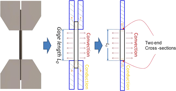
Heat transfer boundary conditions in the real experiment and in the model

The volume average heat source \( (g_{\text{av}} (t) = \int_{V} {g({\bf x},t)dv} \)) of Eq 2 includes the latent heat (l 0 per unit volume) and hysteresis heat (D per unit volume). By assumption (1), we can write the latent heat (l 0) release rate as \( \frac{{l_{0} \upomega }}{2} \cdot \sin (\upomega t) \) which satisfies the condition that the integral of the latent heat release in loading and in unloading is l 0 and −l 0, respectively (i.e., \( \int_{0}^{{\frac{{t_{\text{p}} }}{2}}} {\frac{{l_{0} \upomega }}{2} \cdot \sin (\upomega t)}dt = - \int_{{\frac{{t_{\text{p}} }}{2}}}^{{t_{\text{p}} }} {\frac{{l_{0} \upomega }}{2} \cdot \sin (\upomega t)}dt = l_{0} \)). We can write the hysteresis heat release rate as \( \frac{D\upomega }{\uppi } \cdot \sin^{2} (\upomega t) \) to insure that the integrals of the heat release during loading and unloading are D/2, respectively, (i.e., \( \int_{0}^{{t_{\text{p}} }} {\frac{D\upomega }{\uppi } \cdot \sin^{2} (\upomega t)}dt = \int_{0}^{{\frac{{t_{\text{p}} }}{2}}} {\frac{D\upomega }{\uppi } \cdot \sin^{2} (\upomega t)}dt + \int_{{\frac{{t_{\text{p}} }}{2}}}^{{t_{\text{p}} }} {\frac{D\upomega }{\uppi } \cdot \sin^{2} (\upomega t)}dt = \frac{D}{2} + \frac{D}{2} = D \)). Now, we have
We apply the divergence theorem to transform the volume integral of Eq 2 to a surface integral:
The surface integral \( \int_{S} {k\frac{\partial T}{\partial n}ds} \) includes the heat convection through the wire’s side surface with the heat flow \( Q_{\text{conv}} \left( { = - hA_{\text{side}} \left( {T_{\text{av}} - T_{0} } \right) = - h \cdot 2\uppi RL_{0} \cdot \left( {T_{\text{av}} - T_{0} } \right)} \right) \) and the heat conduction through the two end cross sections with the heat flow \( Q_{\text{cond}} \left( { = - 2kA_{\text{end}} \left| {\frac{{dT_{\text{av}} }}{dx}} \right| = - 2k \cdot \uppi R^{2} \cdot \frac{{\upalpha \left( {T_{\text{av}} - T_{0} } \right)}}{{L_{0} }}} \right), \) T 0 is the temperature of the ambient and \( \upalpha \) is a constant. Now \( \int_{S} {k\frac{\partial T}{\partial n}ds} \) (the total heat flow through the outer surface S) of Eq 8 becomes
In the above, h is the natural convection coefficient of the side surface in air and depends on the temperature difference (Ref 9), \( \overline{h} \) is the lumped effective heat convection coefficient of the side surface (i.e., already including the conduction contribution at the two end cross sections of the wire) and \( \overline{h} = \left( {\frac{2\upalpha k}{{L_{0}^{2} }} + \frac{2h}{R}} \right) \cdot \frac{R}{2} \). It is seen that \( \overline{h} \) decreases with the increase in L 0 and \( \overline{h} \to h \) when \( L_{0} \gg \sqrt {\frac{\upalpha kR}{h}} \). So, with Eq 7 and 9, Eq 2 becomes
For the purpose of simplicity (Ref 7), we have taken \( \overline{h} \) and D in Eq 10 as constants for each frequency of loading. Solving Eq 10 with initial condition \( \left. {T_{\text{av}} } \right|_{t = 0} = T_{0} \), we have
where \( \overline{{t_{h} }} \left( { = \frac{\uplambda R}{{2\overline{h} }}} \right) \) is the characteristic time scale of the lumped effective convection through the side surface. The first term on the right hand side of Eq 11 gives the mean temperature of the specimen in the steady-state cycle, which is caused by the accumulation of the steady-state hysteresis heat (stress-strain loop area) of the phase transition. The second term is the mean temperature variation in the transient stage. It decays exponentially with time t. Its sign depends on the values of l 0, D, λ, ω, \( \overline{{t_{h} }} \). The last term represents the temperature oscillations caused by latent heat and hysteresis heat, respectively.
Comparison with Experimental Data
To check the predictive power of the developed model, the predictions of Eq 11 for two real cyclic loading tests (Ref 7) of trained NiTi superelastic wires (3.5-mm diameter, Johnson Matthey Inc., USA) are shown in Fig. 3. The specific heat capacity of the wire is λ = 3.225 × 10⁶ J/m3·K, the specific latent heat l 0 is 12 J/g, \( \overline{h} = 100\,{\text{W}}/{\text{m}}^{2}{\cdot}{\text{K}} \), and D was the measured steady-state strain-strain hysteresis loop area at given frequency. We can see that the model prediction (red color) not only captures the experimental features but also agrees quantitatively well with the measured temperature variation (blue color) in both transient and steady state stages.

Comparison between the experimental data at frequency (a) 0.1 Hz and (b) 0.4 Hz and modeling results (without fitting parameters) (Color figure online)
Conclusions
We have used the lumped system method to build a simple analytical model to predict the volume average temperature under displacement-controlled cyclic phase transition of a superelastic NiTi wire. From the model, the temperature variation of the specimen can be treated as the superposition of the temperature oscillation over the mean temperature. The oscillation is mainly caused by the latent heat release/absorption during the forward/reverse phase transition, while the mean temperature rise \(( \frac{{D\overline{{t_{h}}} \upomega }}{2\uppi \uplambda }) \) of the specimen is caused by the accumulation of hysteresis heat in the cyclic phase transition. It is revealed that the loading frequency indeed has a significant effect on the thermal response of the material and that, among a set of internal and external parameters, it is the ratio of the characteristic time scale of heat transfer \( \overline{{t_{h} }} \) over the characteristic loading time (t p = 2π/ω) that controls the temperature variation. The predictions of the model (without any fitting parameters) agree well with the experiment results. The results and the modeling methodology of this paper can be applied to the temperature variation of other specimen geometries and ambient conditions.
References
J.A. Shaw and S. Kyriakides, Thermomechanical Aspects of NiTi, J. Mech. Phys. Solids, 1995, 43(8), p 1243–1281
Y. He, H. Yin, R. Zhou, and Q.P. Sun, Ambient Effect on Damping Peak of NiTi Shape Memory Alloy, Mater. Lett., 2010, 64(13), p 1483–1486
Y.J. He and Q.P. Sun, Frequency-Dependent Temperature Evolution in NiTi Shape Memory Alloy Under Cyclic Loading, Smart Mater. Struct., 2011, 19(11), 115014 (9pp)
C. Morin, Z. Moumni, and W. Zaki, A Constitutive Model for Shape Memory Alloys Accounting for Thermomechanical Coupling, Int. J. Plast., 2011, 27(5), p 748–767
H. Soul, A. Isalgue, A. Yawny, V. Torra, and F.C. Lovey, Pseudoelastic fatigue of NiTi wires: frequency and size effects on damping capacity, Smart mater. Struct., 19(8), 085006 (7pp)
S. Miyazaki, T. Imai, Y. Igo, and K. Otska, Effect of Cyclic Deformation on the Pseudoelasticity Characteristics of Ti-Ni Alloys, Metall. Trans. A, 1986, 17(1), p 115–120
H. Yin, PhD thesis, The Hong Kong University of Science and Technology, 2012
R.M. Cotta and M.D. Mikhailov, Heat Conduction: Lumped Analysis, Integral Transforms, Symbolic Computation, John Wiley & Sons, New York, 1997
J.P. Holman, Heat Transfer, 9th ed., McGraw-Hill, New York, 2002
X. Zhang, P. Feng, Y.J. He, T.X. Yu, and Q.P. Sun, Experimental Study on Rate Dependence of Macroscopic Domain and Stress Hysteresis in NiTi Shape Memory Alloy Strips, Int. J. Mech. Sci., 2010, 52, p 1660–1670
Author information
Authors and Affiliations
Corresponding author
Rights and permissions
About this article
Cite this article
Yin, H., Sun, Q. Temperature Variation in NiTi Shape Memory Alloy During Cyclic Phase Transition. J. of Materi Eng and Perform 21, 2505–2508 (2012). https://doi.org/10.1007/s11665-012-0395-9
Received:
Revised:
Published:
Issue Date:
DOI: https://doi.org/10.1007/s11665-012-0395-9