Network malware classification comparison using DPI and flow packet headers

Abstract

In order to counter cyber-attacks and digital threats, security experts must generate, share, and exploit cyber-threat intelligence generated from malware. In this research, we address the problem of fingerprinting maliciousness of traffic for the purpose of detection and classification. We aim first at fingerprinting maliciousness by using two approaches: Deep Packet Inspection (DPI) and IP packet headers classification. To this end, we consider malicious traffic generated from dynamic malware analysis as traffic maliciousness ground truth. In light of this assumption, we present how these two approaches are used to detect and attribute maliciousness to different threats. In this work, we study the positive and negative aspects for Deep Packet Inspection and IP packet headers classification. We evaluate each approach based on its detection and attribution accuracy as well as their level of complexity. The outcomes of both approaches have shown promising results in terms of detection; they are good candidates to constitute a synergy to elaborate or corroborate detection systems in terms of run-time speed and classification precision.

1 Introduction

We present a combined study using data mining techniques to classify malicious packets produced by malware comparing the header approach and full packets classification and compare their strengths and weaknesses. The primary intent of both approaches is to detect malicious traffic at the network level. In [11], authors showed that singular packet headers can be used to fingerprint maliciousness at the network level. In this paper, we extend the aforementioned research by using flow packet headers to detect and attribute malware families (see Section 4.2.1 and Appendix 9), as well as investigating DPI-based maliciousness fingerprinting capabilities.

1.1 Motivations

Perpetrating cyber-attacks negatively impacts organizations as well as individual people. In the recent past, IT security experts have observed a rise in cyber-attacks against individuals, corporations, and government organizations. Hackers tend to elaborate more sophisticated attacking and threatening tools. Malware are frequently subjected to metamorphosis and are targeting more sensitive networks. For instance, vulnerabilities have been discovered in infrastructures controlled by SCADA systems. These systems can control nuclear energy, water distribution, and electricity systems. A particular malware known as Flame [14] has infected computers linked to SCADA systems mainly in Middle Eastern countries. This malware can spread through local networks or USB keys. It has the ability to record screenshots, keystrokes, and Skype conversations, and can change the behavior of industrial controllers. According to Kaspersky, Flame struck approximately one thousand machines [107] including those belonging to government organizations, universities, and individuals. In this context, the detection of malicious traffic generated from infected machines or command and control servers is of paramount importance for the early interception and mitigation of these attacks.

1.2 Contributions

• 1. Packet Headers Flow Based Fingerprinting: Detection.

  We use flow packet headers for the purpose of malicious traffic detection. To do so, we apply several machine learning techniques to build classifiers that fingerprint maliciousness on IP traffic. As such, J48, Naïve Bayesian, SVM and Boosting algorithms are used to classify malware communications that are generated from dynamic malware analysis. Generated network traces are re-processed to eliminate noisy traffic and extract traffic that is considered as a maliciousness ground truth. This traffic is used to collect attributes from bidirectional flows packet headers. These attributes aim to characterize maliciousness in flows. Data mining algorithms are applied on these features. The comparison between different algorithm results has shown that J48 and Boosted J48 algorithms have performed better than other algorithms. We obtained a detection rate of $99\%$ with a false positive rate less than $1\%$ for J48 and Boosted J48 algorithms. The experiments have been conducted on many benign datasets, representing a residential setting, a research laboratory, an ISP edge router and a private company.

• 2. Packet Headers Flow Based Fingerprinting: Attribution.

  In addition to detecting maliciousness using flow attributes collected from packet headers, we aim to corroborate fingerprinting capability with malware families’ attribution using Hidden Markov Models (HMMs). To do so, we use a clustering approach to label inbound and outbound unidirectional flows. Similar to the detection approach, the clustering takes as input flow attributes obtained from packet headers. However, the attributes are extracted from unidirectional flows instead of bidirectional flows. The reason for this is that we do not want to lose the semantics of traffic direction when we characterize malicious traffic. Once the different unidirectional flows are labeled, we derive sequences of malicious flows and index them per malware family. These sequences of malicious flows are used through an iterative process to build HMMs representing malware families. HMMs mirror the behavior of malware families at the network level. We conduct the experiment on 294 malware families and generate profiling models for each malware family.

• 3. Signal and NLP DPI Fingerprinting: Detection and Attribution.

  In the second approach, namely, DPI, we apply machine learning techniques on complete packet captures (pcaps). The intent is to fingerprint malicious packets by using MARF open-source [55] framework and its MARFPCAT application (originally based on MARFCAT, designed for the SATE static analysis tool exposition workshop it was used to machine-learn, detect, and classify vulnerable or weak code quickly and with relatively high precision). Initially, we train models based on malware pcap data to measure detection accuracy. Then, we test obtained models on unseen labeled data. It is important to mention that the training and testing phases are based on combining many machine learning techniques [58] to select the best options. In this work, we elaborate on the details of the methodology and the corresponding results. We applied signal processing and natural-language processing (NLP) machine learning techniques to analyze and detect maliciousness in pcap traces. Being inspired by the works introduced in [57] to detect and classify vulnerable and weak code (Java bytecode and C object code) with a relatively high precision, we integrated a proof-of-concept tool, namely, MARFPCAT, a MARF-based PCAP Analysis Tool, which is used to train 70% different malware network traces and measure the precision on remaining network traces. It is important to mention that training and testing data are indexed per malware family.

• 4. Comparison of Both Approaches.

  In this paper, we address the issue of malicious IP traffic detection. As a requirement, we formulate the following objectives: (1) detection of malicious IP traffic even in the presence of encryption, and (2) scalable detection. To this end, we initiated research to fingerprint maliciousness at the level of network traffic. Thus, we present a comparative study between fingerprinting maliciousness based on Deep Packet Inspection (DPI) and high-level properties of flows (flow packet headers). In this context, we put forward an attempt to answer the following questions:

  • How to fingerprint maliciousness at the IP traffic level using the properties of flow packet headers?

  • How to fingerprint maliciousness at the IP traffic level using DPI?

  • What are the advantages and drawbacks for each approach?

  Looking at the problem of detection and classification from another perspective, we obtain the maliciousness ground truth from network traces generated from dynamic malware analysis. We exploit the fact that these traces are generated from a large set of malware families to infer maliciousness through machine learning algorithms. The availability of detection tools would help network security experts to discover infected machines or the existence of botnet communication generated from command-and-control servers as well as uploads and downloads from deposits of stolen information. While Intrusion Detection Systems (IDSs) are cornerstones among defense artifacts to protect computer networks, they lack the necessary strength to cope with encrypted traffic as well as large traffic volumes. As such, there is an objective to fingerprint maliciousness in IP traffic through the classification of either DPI, packet headers, or both, in order to achieve higher confidence levels. A comparative study for both approaches is a vital necessity to grasp the dynamics to fingerprint maliciousness at the IP traffic level.

2 Related work

The pure-packet content approach has shown good results in terms of malware detection at the network level, but it fails in capturing maliciousness when the traffic is encrypted. Moreover, it requires sampling to preserve scalable detection in the presence of a large amount of traffic. Our first approach is malware network behavior-based rather than content-based to avoid these two limitations. Our second approach treats the whole packet, including headers and the payload, for the same task. Both approaches rely on machine learning and various data processing algorithms detailed in the methodology aiming to ascertain the common characteristics shared by malicious flows at the network level. Subsequently, we introduce the related works related to the identification of maliciousness using a malware network behavioral approach. In the sequel, we present the different related works, which span over: (1) Network Traffic Analysis and (2) Malware Analysis and Classification.

2.1 Network traffic analysis

Data mining techniques have been used in the analysis of network traffic for many purposes, i.e., application protocols fingerprinting, anomaly detection for intrusion and zero-day attacks identification. In protocols fingerprinting, many research efforts have been proposed. For instance, Density Based Spacial Clustering of Application with Noise was proposed [102] in 2008 to use clustering algorithms to identify various FTP clients, VLC media player, and UltraVNC traffic over encrypted channels. Li et al. [44] used wavelet transforms and k-means classification to identify communicating applications on a network. Alshammari et al. [4, 5] put forward research efforts to identify ssh and Skype encrypted traffic (without looking at payload, port numbers, and IP addresses). Additionally, comparison of algorithms and approaches for network traffic classification were proposed separately by Alshammari et al. [3] in 2008 and Okada et al. [68] in 2011, surveying and comparing various machine learning algorithms for encrypted traffic analysis.

In addition to application protocols fingerprinting, many research efforts have been introduced to identify anomalies in traffic for the purpose of intrusion and malicious traffic detection. In 2000, Lee et al. [43] introduced a data mining approach for the purpose of intrusion detection. They described a data mining framework, which leverages system audit data as well as relevant system features to build classifiers that recognize anomalies and known intrusions. Bloedorn et al. [9] in 2001 described data mining techniques needed to detect intrusions along with needed expertise and infrastructure. Fan et al. [18] proposed an algorithm to generate artificial anomalies to force the inductive learner to segregate between known classes (normal traffic and intrusions) and anomalies. In [90], the authors provided an overview of Columbia IDS Project, where they presented the different techniques used to build intrusion detection systems. In [42], Lee reported on mining patterns from system and network audit data, and constructing features for the purpose of intrusion events identification. This work provided an open discussion about research problems that can be tackled with data mining techniques. Locasto et al. [48, 49] brought the use of collaborative security at the level of intrusion detection systems. They proposed a system that distributes alerts to collaborative peers. They integrated a component that extracts information from alerts and encodes it then in Bloom filters. Another component is used to schedule correlation relationships between peers.

In [98], Wang et al. integrated a tool, namely, PAYL, which models the normal application payload of network traffic. The authors used a profile byte distribution and standard deviation for hosts and ports to train the detection model. They took advantage of Mahalanobis distance to compute the similarity of testing data against pre-computed profiles. If the distance exceeds a certain threshold, the alert is generated. Zanero et al. [105] presented a hybrid approach, which lies in: (1) an unsupervised clustering algorithm to reduce network packets payload to a tractable size, and (2) an anomaly detection algorithm, to identify malformed and suspicious payloads in packets and flow of packets. In the same spirit of aforementioned work, Zanero showed explicitly in [104] how Self Organizing Map algorithm (SOM) is used to identify outliers on the payload of TCP network packets. In [106], Zanero et al. extended their work by introducing approximate techniques to speed up the SOM algorithm at runtime. They provided more elaborated results and compared their work with existing systems. In [94], the authors depicted Payload Content based Network Anomaly Detection (PCNAD), which a corroboration to PAYL system. They used Content-based Payload Partitioning (CPP) to divide the payload into different partitions. The subsequent anomaly analysis is performed on partitions of packet payloads. They showed that PCNAD has a high accuracy in terms of anomaly detection on port 80 by using only $62.64\%$ of packet payload length. Perdisci et al. [74] presented the multiple classifier payload-based anomaly detector (McPAD). Like PAYL system, the authors use n-grams but with features reduction to avoid the curse of the dimensionality problem [17]. They applied a feature clustering algorithm proposed in [15] for text classification to reduce features. McPAD detects network attacks having shell-code in the malicious payload as well as some advanced polymorphic attacks.

Song et al. [88] introduced Spectrogram to detect attacks against web-layer code-injection (e.g., PHP file inclusion, SQL-injection, XSS attacks, and memory-layer exploits). They built a sensor that builds dynamically packets to construct content flows and learns to recognize legitimate inputs in web-layer scripts. They used the Mixture-of-Markov-Chains to train a model that detect anomalies in web-content traffic. Golovko et al. [22] discussed the use of neural networks and Artificial Immune Systems (AIS) to detect malicious behavior. The authors studied the integration and the combination of neural networks in modular neural systems to detect malware and intrusions. They proposed a multi-neural network approaches to detect probing, DoS, user-to-root attacks, and remote-to-user attacks. In [10], Boggs et al. elaborated on a system that detects zero-day attacks. The authors correlated web requests containing user submitted data considered abnormal by Content Anomaly Detection (CAD) sensors. Boggs et al. filtered the requests with high entropy to reduce data processing overhead and time. They evaluated their correlation working prototype with data collected during eleven weeks from production web servers. Whalen et al. [99], adapted outlier detection to cloud computing. The authors proposed an aggregation method where they use random forest, logistic regression, and bloom filter-based classifiers. They showed the scalability of their proposed aggregation content anomaly detection with indistinguishable detection performance in comparison with content anomaly detection classical methods.

As being the first step of an attack’s vector, network scanning (reconnaissance) has been the target of many research efforts. For instance, Simon et al. [84] formalized the scanning detection as a data-mining problem. They converted collected datasets as a set of features to run off-the-shelf classifiers, like Ripper classifier, on. They showed that the data-mining models encapsulate expert knowledge that outperform in terms of coverage and precision in scanning identification. The emergence of botnets and malicious content delivery networks has pushed researchers to investigate the identification and detection of such networks. For example, in [8, 47], authors put forward methods to detect IRC botnets. In [8], Binkley et al. presented an anomaly-based algorithm to detect IRC-based botnet meshes. The algorithm uses a TCP scan detection heuristic (TCP work weight) and other collected statistics gathered on individual IRC hosts. The algorithm sorts the channels by the number of scanners producing a list of potential botnets. The authors deployed a prototype in a DMZ and managed to reduce the number of botnet clients. In [47], Livadas et al. presented machine learning-based classification techniques to identify the command-and-control (C&C) traffic of IRC-based botnets. They proposed a two-stages detection system. The first stage consists of distinguishing between IRC and non-IRC traffic, whereas the second lies in segregating botnet and real IRC traffic. In [31], Karasaridis et al. put forward an approach to identify botnet C&Cs by combining heuristics characterizing IRC flows, scanning activities, and botnet communications. They used non-intrusive algorithms that analyze transport layer data and do not rely on application layer information.

In [23], Gu et al. introduced BotHunter, which models all bot attacks as a vector enclosing scanning activities, infection exploits, binary download and execution, and C&Cs communication. The tool was coupled with Snort [89] IDS with malware extensions to raise alerts when different bot activities are detected. Based on statistical payload anomaly detection, statistical scan anomaly detection engines and rule-based detection, BotHunter correlates payload anomalies, inbound malware scans, outbound scans, exploits, downloads and C&C traffic and produces bot infection profiles. In [24], Gu et al. used aggregation technique to detect botnets. They explained how bot infected hosts have spatial-temporal similarity. They introduced BotSniffer, which is a system that pinpoints to suspicious hosts that have malicious activities such as sending emails, scanning, and shared communication payloads in IRC and HTTP botnets by using shared bi-grams technique. In [25], Gu et al. exposed BotMiner, which aims to identify and cluster hosts that share common characteristics. It consists of two traffic monitors (C-plane and A-plane monitors) deployed at the edge of network. The C-plane monitor logs network flows in a format suitable for storage and analysis. The A-plane monitor detects scanning, spamming, and exploit attempts. The clustering components (C-plane clustering and A-plane clustering components) process the logs generated by the monitors to group machines that show very similar communication patterns and activity. The cross-plane correlator combines the results and produces a final decision on machines that belong to botnets.

Another noticeable research using aggregation technique was introduced in [103], where Yen et al. presented TAMD, an enterprise network monitoring prototype that identifies groups of infected machines by finding new communication flows that share common characteristics (communication “aggregates”) involving multiple network internal hosts. Their characteristics span over flows that communicate with the same external network, flows that share similar payload, and flows that involve internal hosts with similar software platforms. TAMD has an aggregation function, which takes as input a collection of flow records and outputs groups of internal hosts having a similarity value based on the input flow record collections. To reduce the dimensionality of vectors representing hosts, the authors used Principal Component Analysis (PCA). To cluster different hosts, authors used k-means algorithm on reduced vectors. In [13], Chang et al. proposed a technique that detects P2P botnets C&C channels. They considered a clustering approach (agglomerative clustering with Jaccard Similarity criterion function) to capture nodes’ behavior on the network, then, they used statistical tests to detect C&C behavior by comparing it with normal behavior clusters. In [67], Noh et al. also defined a method to detect P2P botnets. They focused on the fact that a peer bot generates multiple traffic traces to communicate with large number of remote peers. They considered that botnet flows have similar patterns, which take place at irregular intervals. They used a flows grouping technique, where a probability-based matrix is used to construct a transition model. The features representing a flow state are protocol, port, and traffic. A likelihood ratio is used to detect potential misbehavior-based transition information in state values. In [92], the authors introduced a novel system, BotFinder, which detects infected hosts in a network by considering high-level properties of the botnet network traffic. It uses machine learning to identify key features of C&C communication based on bots traffic produced in a controlled environment. Our approach has the same flavor of BotFinder; however, we create a detection model based on machine learning techniques by considering not only bots, but any malware type. In [16], Dietrich et al. introduced CoCoSpot, which recognizes botnet C&Cs channels based on carrier protocol distinction, message length sequences and encoding differences. The authors used average-linkage hierarchical clustering to build clusters of C&C flows. These clusters are then used as knowledge base to recognize potentially unknown C&C flows.

2.2 Malware analysis and classification

In addition to network analysis for the purpose of malicious and intrusion traffic detection described earlier, many research efforts have emerged to tackle malware classification. Part of our methodology shares some similarities with the related work on automatic classification of new, unknown malware and malware in general, such as viruses, web malware, worms, spyware, and others where pattern recognition and expert system techniques are successfully used for automatic classification [59]. Malware classification falls into system-based classification and network-based classification. Regarding the first strand, Schultz et al. [82] proposed a data-mining framework that automatically detects malicious executables based on patterns observed on some malware samples. The authors considered a set of system-based features to train classifiers, such as inductive rule-based learner (Ripper), which generates Boolean rules, and a probabilistic method that computes class probabilities based on a set of features. A multi-classifier system combines the outputs from several classifiers to generate a prediction score. In [6], Bailey et al. proposed a behavioral classification of malware binaries based on system state changes. They devised a method to automatically categorize malware profiles into groups that have similar behaviors. They demonstrated how their clustering technique helps to classify and analyze Internet malware in an effective way. Rieck et al. [77] aimed to exploit shared behavioral patterns to classify malware families. The authors monitored malware samples in a sandbox environment to build a corpus of malware labeled by an anti-virus. The corpus is used to train a malware behavior classifier. The authors ranked discriminative features to segregate between malware families. In [96], Trinius et al. introduced Malware Instruction Set (MIST), which is a representation of malware behavior. This representation is optimized to ease and scale the use of machine learning techniques to classify malware families based on their behavior. Bayer et al. [7] put forward a scalable clustering approach to group malware exhibiting similar system behavior. They performed dynamic malware analysis to collect malware execution traces. These traces are transformed to profiles (features set). The authors used Locality Sensitive Hashing (LSH) to hash features values and improved scalability of profiles hierarchical clustering.

Wicherski [100] introduced a scalable hashing non-cryptographic method to represent binaries using a portable executable format. The hashing function has the ability to group malware having multiple instances of the same polymorphic specimen into clusters. Hu et al. [29] implemented and evaluated a scalable framework, namely, MutantX-S, that clusters malware samples into malware families based on programs’ static features. The program is represented as set of opcodes sequence easing the extraction of n-gram features. The dimensionality of vectors representing the features is reduced through a hashing function. Regarding malware network-based profiling and classification, Rossow et al. [79] provided a comprehensive overview about malware network behavior obtained through the use of Sandnet tool. The authors conducted an in-depth analysis of the most popular protocols that are used by malware, such as DNS and HTTP. Nari and Ghorbani [66] classified malware samples based on network behavior of malware. Their approach transforms pcap files representing malware families into a protocol based behavioral graph. The features (graph size, root out-degree, average out-degree, maximum out-degree, number of specific nodes) are extracted from these graphs and a J48 classifier was used to classify malware families. In [34], Kheir et al. presented WebVisor, a tool that derives patterns from Hypertext Transfer Protocol (HTTP) C&C channels. The tool builds clusters based on statistical features extracted from URLs obtained from malware analysis. The approach is a fine-grained, noise-agnostic clustering process, which groups URLs for the purpose of malware families attribution.

2.3 Static analysis

Being inspired by machine learning techniques used for the detection of security-weak, vulnerable or malicious code we use to some extend the same techniques in fingerprinting maliciousness through our DPI approach (Section 5). We are motivated by the fact that such techniques can detect and classify malware-specific payload in the network traffic regardless the packet size or architecture very fast. In the sequel, we list the different related works where machine learning techniques were used to detect flaws in the static analysis of code. In [38–40], Engler’s team proposed the use of statistical analysis, ranking, approximation, dealing with uncertainty, and specification inference in static code analysis. Encouraged by the statistical NLP techniques such as the ones described in [50], research efforts have been proposed to detect vulnerabilities in static code. Arguably, the first time that a research effort attempted to classify vulnerable/weak code, was in 2010. The first results were demonstrated in SATE2010 workshop [69], where the MARFCAT project [57, 62, 63] demonstrated promising results. In the prevailing of what was presented at the SATE2010 workshop and the fact that MARF has the ability apply machine learning techniques for quick scans of large collection of files [59], the authors used core ideas and principles behind the MARF’s pipeline to test various algorithms and expose results. A similar approach was introduced in [12]. There, the authors classify and predict vulnerabilities by using SVMs. BitBlaze (and its web counterpart, WebBlaze) are two other recent tools that perform fast static and dynamic binary code analysis for vulnerabilities, developed at Berkeley [86, 87]. Kirat et al. introduced their tool SigMal to do static signal processing analysis of malware [35].

3 Maliciousness ground truth

We execute collected malware samples in a controlled environment (sandbox) to generate representative malicious traffic. This is used as a ground truth for maliciousness fingerprinting. The sandbox is based on a client-server architecture, where the server sends malware to clients. It is important to mention that the dynamic analysis setup allows malware to connect to the Internet to generate inbound/outbound malicious traffic. Figure 1 illustrates the dynamic malware analysis topology. We receive an average of 4, 560 malware samples on a daily basis from a third party. We execute the malware samples in the sandbox for three minutes. We chose this running period to make sure that we can handle up to 14, 400 malware runs per day. The period gives the ability to run all malware samples with a re-submission. The latter is important in case where malware do not generate network traffic during the initial runs. For each run, a client monitors the behavior of each malware and records it into report files. These files contain malware activities such as file activities, hooking activities, network activities, process activities, and registry activities. The setup of dynamic malware analysis lies in a network, which is composed of a server and 30 client machines. The server runs with an Intel(R) Core$^{TM}$ i7 920@2.67 GHz, Ubuntu 11 64 bit operating system and 12.00 GB of physical memory (RAM). Each client runs with an Intel(R) Core$^{TM}$ 2 6600@2.40 GHz, Microsoft Windows XP Professional 32-bit operating system and 1.00 GB of physical memory. Such physical machines are used for the reason that some malware cannot run in virtual machines. As a downstream outcome of the aforementioned dynamic analysis, we gathered the underlying traffic pcap files that were generated. The dynamic malware analysis has generated approximately 100, 000 pcap files labeled with the hashes of malware, which corresponds to a size of 3.6 GB. In our work, we considered inbound and outbound traffic generated by malware labeled by Kaspersky malware naming schema. The reasons behind using this naming schema are as follows: (1) We noticed that it manages to cover the naming of the majority of malware samples considered in experiments. (2) The malware naming provided by Kaspersky follows the malware convention name (Type.Platform.Family.Variant). The number of bidirectional flows is 96, 235 and the number of unidirectional flows is 115, 000.

Fig. 1

Dynamic Malware Analysis Topology

4 Packet headers flow based fingerprinting

In this section, we describe how packet headers flow fingerprinting is done. By fingerprinting, we mean (1) malicious traffic detection and (2) malware family attribution. First, for detection, we extract bidirectional flow features from malicious traces generated from dynamic malware analysis, together with benign traces collected from trusted third parties. These features are used by classification algorithms to create models that segregate malicious from benign traffic (see Section 4.1.1). Regarding attribution, we elaborate non-deterministic malware family attribution based on Hidden Markov Models (HMMs). The attribution is done through probabilistic scores for different sequences of malicious labeled unidirectional flows. The obtained models act as probabilistic signatures characterizing malware families.

4.1 Malicious traffic detection

Malicious traffic detection’s goal is to isolate malicious communication sessions. These sessions include flows used to perform various malicious activities (e.g., malware payload delivery, DDoS, credentials theft). These flows are usually intermingled with a large portion of IP traffic that corresponds to benign activities over computer networks. As such, maliciousness detection amounts to the segregation of malicious from benign flows. To this end, we represent flows through a set of attributes (features) that capture their network behaviors. By leveraging these features, we create classifiers that automatically generate models to detect malicious traffic. With this in mind, we define four phases to infer maliciousness at the network level: selecting and extracting the bidirectional flow features, labeling of the traffic (malicious and benign), training the machine learning algorithms, and evaluating the classifiers produced by these algorithms. Figure 2 illustrates how detection of maliciousness is performed.

Fig. 2

Flow Based Detection Approach

4.1.1 Benign traffic datasets

For the purpose of building a classification model that distinguishes between malicious and benign traffic, we collected benign traffic from WISNET [101] and private companies. These datasets have been built to evaluate Intrusion Detection Systems in terms of false alerts and to detect anomalies in network traffic. In our work, we use such datasets to build baseline knowledge for benign traffic. These datasets have been used together with the malicious traffic dataset to assess classification algorithms in terms of accuracy, false positives and negatives. Table 1 shows the number of benign flows in each dataset. The different datasets used in this work illustrates four different location datasets, namely, residential setting, research laboratory, ISP edge router and private company networks.

Table 1 Benign Datasets

4.1.2 Bidirectional flow features extraction

We capture malicious network traces from the execution of malware binaries in the ThreatTrack sandbox [95]. We label these traces accordingly as malicious, while the clean traffic traces obtained from trusted third parties [101] are labeled as benign. Flow features are extracted from these labeled network traces to capture the characteristics of malicious and benign traffic. It is important to mention that these features can be extracted even when the traffic is encrypted, as they are derived from flow packets headers. The flow features exploited are mainly based on flow duration, direction, inter-arrival time, number of exchanged packets, and packets size.

A bidirectional flow is a sequence of IP packets that share the 5-TCP-tuple (source IP, destination IP, source port number, destination port number, protocol). The outbound traffic is represented by the forward direction, while the backward direction represents the inbound traffic. In terms of design and implementation, the module in charge of network traces parsing, labeling, and feature extraction reads network streams using jNetPcap API [85], which decodes captured network flows in real-time or offline. This module produces values for different features from network flows. The resulted values are stored in features files that are provided to Weka [93]. The network traces parser represents each flow by a vector of 22 flow features. Table 2 illustrates the description of the bidirectional flow features.

Table 2 Bidirectional Flow Features

4.1.3 Traffic classification

The feature files resulting from the previous phase are provided as input to classification algorithms. The intent is to build models that have the ability to distinguish between malicious and benign flows. To this end, we use machine learning algorithms, namely, Boosted J48, J48, Naïve Bayesian, Boosted Naïve Bayesian, and SVMs. The classification module is based on a Java wrapper that runs these machine learning algorithms. The module has two execution phases: learning and testing. In the learning phase, we build the classifier using 70% of malicious and benign traces. In the testing phase, we evaluate the classifier with the rest of the data (30%). It is important to mention that training and testing datasets do not overlap with each other. In the sequel, we give a brief overview of the classification algorithms.

J48 Algorithm: It is Java implementation of C4.5 classification algorithm [75]. J48 [19] builds the tree by dividing the training data space into local regions in recursive splits. The split is pure if all observations in a decision branch belong to the same class. To split the training dataset, J48 computes the goodness of each attribute (feature) to be the root of a decision branch. It begins by computing the information need factor. The J48 algorithm splits recursively datasets to sub-datasets and computes the information need per feature. If the split is not pure (presence of many classes), the same process will be used to split the sub-dataset into pure classes. The split stops if each sub-dataset belongs to one class (pure split). The decision tree result is composed of nodes (the attributes) and terminal leaves (classes). That will be used to identify the unseen data when the model is deployed [27].

Naïve Bayesian Algorithm: It is based on Bayes’ theorem [27]. It is a statistical classifier, which outputs a set of probabilities that show how likely a tuple (observation) may belong to a specific class [27]. Naïve Bayesian assumes that the attributes are mutually independent. Naïve Bayesian starts by computing the probability of an observation. Once the probabilities are computed, Naïve Bayesian associates each observation with the class that has the higher probability with it. Naïve Bayesian is an incremental classifier, which means that each training sample will increase or decrease the probability that a hypothesis is correct.

Boosting Algorithm: It is a method used to construct a strong classifier from a weak learning algorithm. Given a training dataset, boosting algorithm incrementally builds the strong classifier from multi-instances of a weak learning machine algorithm [21]. Boosting algorithm takes, as input, the training dataset and the weak learning algorithm. It divides the training dataset into many sub-datasets $(x_1, y_1) ,...,(x_i, y_j)$, where $x_i$ belongs to X (a set of observations) and $y_j$ belongs to Y (set of class attribute values), and calls the weak learning algorithm to build the model for each sub-dataset. The resulted models are called decision stumps. The latter examine the features and return the decision tree with two leaves either $+1$ if the observation is in a class, or $-1$ if it is not the case. The leaves are used for binary classification (in case the problem is multi-classes, the leaves are classes). Boosting algorithm uses the majority voting schema between decision stumps to build a stronger model.

SVM Algorithm: The Support Vector Machines (SVM) [20, 28] algorithm is designed for discrimination, which is meant for prediction and classification of qualitative variables (features) [70]. The basic idea is to represent the data in a landmark, where the different axes are represented by the features. The SVM algorithm constructs a hyper-plane or set of hyper-planes in a high-dimensional. Then, it searches for the hyper-plane that has the largest distance to the nearest training data points of any class. The larger is the distance, the lower is the error of the classification.

4.2 Malicious traffic attribution

The attribution of malicious traffic to malware families corroborates detection since it (1) shifts the anti-malware industry from the system level to the network level, and (2) eases the mitigation of infected machines. It gives the ability to networking staff to undertake actions against botnets, depots of stolen information, spammers, etc. For instance, if an administrator notices the presence of malicious traffic in the network, and this traffic can be attributed to a bot family. He/She responds to the threat by blocking malicious connections and quarantine infected machines for a removal of malware. Thus, to enhance maliciousness fingerprinting at the network level, we decide to integrate the malware family attribution. To do so, we use network traces obtained from dynamic malware analysis and index them with malware families. For each set of traces belonging to a malware family, we extract sequences of unidirectional flows. These flows are labeled through a clustering method. The labeled sequences obtained are used to train HMMs for different malware families. Figure 3 illustrates how malware families’ attribution is performed.

Fig. 3

Non-Deterministic Approach for Malware Family Attribution

4.2.1 Malware family indexation

As a downstream outcome of dynamic malware analysis, we collect approximately 100, 000 network traces (pcap files). Each trace is labeled by the corresponding malware sample hash. We use Kaspersky malware name schema to recognize the malware family of each hash (see example malware families in tables in Appendix 9). Subsequently, we index network traces based on their malware family. In this work, we obtain 294 malware families.

4.2.2 Sequencing flows

For each malware family, we browse collected network traces to extract unidirectional flows. These flows fall into inbound and outbound flows, which are used to build sequences of flows. For each sequence, a flow precedes another flow if its timestamp occurrence precedes the timestamp of the following flow. As a result, the sequences are indexed by the corresponding malware family.

4.2.3 Labeling sequences

In order to label different flows belonging to a sequence, we adopt a clustering approach. The reason behind doing so is to characterize outbound and inbound malicious flows into clusters representing their network behaviors. To do so, we represent flows by vectors of 45 features. Table 3 illustrates unidirectional flow features. To perform clustering of inbound/outbound traffic, we generate feature files that are readable by CLUTO clustering toolkit [32]. This was used in diverse research topics such as information retrieval [111] and fraud detection [73]. To label flows, we use the k-means Repeated Bi-Section algorithm implemented in CLUTO. This algorithm belongs to partitional clustering algorithms. These algorithms are known to perform in clustering large datasets since they have low computational cost [2, 41]. k-means RBS derives clustering solutions based on a global criterion function [109]. This algorithm initially creates 2 groups; each group is then bisected until the criterion function is optimized. The k-means RBS algorithm uses the vector space model [80] to represent each unidirectional flow. Each flow is represented by a dimension vector $fv = (f_1, f_2, \ldots , f_i)$, where $f_i$ is the $i^{th}$ unidirectional flow feature. To compute similarity between vectors, we use the cosine function [80]. In order to cluster different unidirectional flows, we use a hybrid criterion function that is based on an internal function and an external function. The internal function tries to maximize the average pairwise similarities between flows that are assigned to each cluster. Unlike the internal criterion function, the external function derives the solution by optimizing a solution that is based on how the various clusters are different from each other. The hybrid function combines external and internal functions to simultaneously optimize both of them. Based on the k-means RBS algorithm, we create a set of experiments: inbound flow clustering solutions and outbound flow clustering solutions. We choose a solution where the internal similarity metric (ISIM) is high and the external similarity metric (ESIM) is moderate.

Table 3 Unidirectional Flow Features

4.2.4 Hidden markov modeling

Hidden Markov Model (HMM) is a popular statistical tool that models time series or sequential data. In this work, we use HMMs to create non- deterministic models that profile malware families. We want to establish a systematic approach to estimate attribution of unidirectional flow sequences to different malware families. We choose HMMs due to their readability since it allows sequences to be significantly interpreted, represented, and scored. We observe that collected flows have different length, and therefore decide to train HMMs based on sub-sequences with fixed length m. In order to fix the number of states in HMMs, we set a sliding window n to represent different combinations of inbound and outbound flows. For instance, if we want HMM states to represent singular flow, there exist two possibilities: IN and OUT. If we want HMM states to represent a sequence of two flows, there are four possibilities: IN / IN, IN / OUT, OUT / OUT and OUT / IN. Similarly, if we want HMM states to represent a sequence of n flows, we obtain $2^n$ states. To train HMMs for each malware family with corresponding sequences, we use the Expectation Maximization (EM) algorithm [54] integrated in the HMMall toolbox for MATLAB [65] to learn hidden parameters of each $2^n$ state HMM representing a malware family. The EM algorithm aims to find the maximum likelihood of parameters of a model where its equations cannot be solved. HMMs usually involve unknown parameters (hidden parameters for HMMs) and known data observations (malicious flows sub-sequences).

4.2.5 Hidden markov models initialization

To create models for different malware families, we initiate baseline HMMs. The states are computed based on a sliding window that we apply on observed sequences. The sliding window allows us to extract sub-sequences from sequences. For instance, for a sequence (a, b, c) and a sliding window of length 2, we obtain sub-sequences (a, b), (b, c). If we consider a HMM based on a sliding window of 1 flow, we result in 2 states HMM since we can have an inbound flow or an outbound flow. If a HMM is based on 2 flows, we obtain 4 states HMM since we can have an inbound/inbound pair, an inbound/outbound pair, an outbound/outbound pair and an outbound/inbound pair. In initialized HMMs, prior probabilities are uniformly distributed over different states. For instance, if we consider a sliding window of length 2, we obtain 4 states HMM with a prior probability of 0.25 for each state. The transition probabilities matrix is initialized such that for each transition between a state $s_i$ and other states, the probabilities are uniformly distributed. If a state has 2 transitions, each transition has a probability of 0.5. The emission probabilities matrix associates a state with an observation vector. Each element of the vector is a probability of observing an inbound or outbound clustering label. For the sake of simplicity, we illustrate in Figures 4a and 4b initialization HMMs for a sliding window length of 1 and 2 respectively. The observation probabilities are uniformly distributed. Let us consider x as the number of input labels and y as the number of output labels. For a 2-states HMM, we associate with the state IN an observation vector, where:

$$\begin{aligned}&\forall i \in \left[ 1,x\right] :\,b(in_i)={1}/{x}\\&\forall j \in \left[ 1,y\right] : \,b(out_j)=0 \end{aligned}$$

Similarly, we associate with the state OUT an observation vector, where:

$$\begin{aligned}&\forall i \in \left[ 1,x\right] :\,b(in_i)=0\\&\forall j \in \left[ 1,y\right] : \,b(out_j)={1}/{y} \end{aligned}$$

For a 4 states HMM, we associate with the state IN / IN an observation vector, where:

$$\begin{aligned}&\forall i \in \left[ 1,x\right] : \,b(in_i)={1}/{x}\\&\forall j \in \left[ 1,y\right] : \,b(out_j)=0 \end{aligned}$$

Similarly, we associate with the state OUT / OUT an observation vector, where:

$$\begin{aligned}&\forall i \in \left[ 1,x\right] : b(in_i)=0\\&\forall j \in \left[ 1,y\right] : \,b(out_j)={1}/{y} \end{aligned}$$

Regarding states OUT / IN and IN / OUT, the observation vector is as follows:

$$\begin{aligned}&\forall i \in \left[ 1,x\right] : \,b(in_i)={1}/{(x+y)}\\&\forall j \in \left[ 1,y\right] : \,b(out_j)={1}/{(x+y)} \end{aligned}$$

Recursively, for a $2^n$ states HMM, the observation vectors are the same as a 4 states HMM. If the states contain IN and OUT, the probabilities are equal to ${1}/{(x+y)}$. If the states contain just IN, the probabilities are equal to 1 / x for all inbound labels and 0 for all outbound labels. Similarly, if the states contain just OUT, the probabilities are equal to 1 / y for all outbound labels and 0 for all inbound labels (Fig. 5).

Fig. 4

HMM States. (a) 2 States Initialization HMM. (b) 4 States Initialization HMM

Fig. 5

MARF’s Pattern-Recognition Pipeline

5 Signal and NLP DPI fingerprinting

In the sequel, we describe the DPI approach to detect maliciousness in the network traffic. The methodology to analyze malicious packets is described in Section 5.1, whereas the different knowledge base machine learning techniques are introduced in Section 5.2. Section 5.3 describes the different steps done to classify packets. In this approach, we look at the packets, including both headers and payloads, as a signal subjected to fast spectral-based classification.

5.1 Core principles

The essence of the whole packet analysis lies in the core principles, which fall into machine learning and Natural Language Processing (NLP) techniques. A set of malicious packets (a network trace) is treated as a data stream signal, where $n$-grams are used to build a sample amplitude value in the signal. In our case, we use bi-grams ($n=2$) (two consecutive characters or bytes) to construct the signal. The reasons behind using bi-grams lay in: (1) it has shown its effectiveness in detecting C&Cs channels [24]; (2) it is adapted to the form of PCI-encoded wave originally integrated in the MARF framework.

Similarly to the aforementioned approach, the whole packet methodology has two phases: (1) the training phase, where MARFPCAT learns from different samples of network traces and generates spectral signatures using signal processing techniques; and (2) the testing phase, where MARFPCAT computes how similar or distant training network traces are from testing network traces. This approach is meant to behave like a signature-based anti-virus or IDS, but using fuzzy signatures. However, we use as much as possible combinations of machine learning and signal processing algorithms to assess their precision and runtime in order to select the best trade-off combination.

At present, we look at complete pcap files, which can affect negatively the MARFPCAT’s malware family attribution accuracy in the presence of encrypted payload. However, MARFPCAT processes network traces quickly since there is no pre-processing of pcap traces (flows identification and extraction). MARFPCAT has the ability to control thresholds of different algorithms, which gives flexibility in selecting classification and the appropriate machine learning techniques.

5.2 The knowledge base

Collected malware database’s behavioral reports and network traces are considered as a knowledge base from which we machine-learn the malicious pcap samples. As such, conducting the experiments fall into three broad steps: (1) Teach the system from the known cases of malware from their pcap data. (2) Test on the known cases. (3) Test on the unseen cases. In order to prepare data for training and testing, we used a Perl script to index pcap traces with malware classes, and we used the same malware naming conventions mentioned earlier. The index is in the form of a meta MARFCAT-IN XML file, which is used by MARFPCAT for training or testing.

In contrast to the packet headers approach, where the benign traffic is collected from third parties; the benign traffic is considered as a noise sample found in pcap traces. To segregate such traffic from the malicious one, we use the low-pass filters and silence compression. In addition, the signal of the benign traffic can be learned and subtracted from malicious traffic (malicious signal) to increase fingerprinting accuracy. However, the latter signal subtraction technique results in decreased run-time performance. Thus, we use only different filters to remove noise from malicious pcaps since the results were very promising without benign traffic subtraction.

5.3 MARFPCAT’s DPI methodology

In this part, we describe the different steps that are performed to fingerprint maliciousness by using DPI approach. Considering this work, we compile annotated manually meta-XML index files with a Perl script. The index file annotates malware network traces (pcaps) indexed by their families. Once the annotation is done, MARF is automatically trained on each pcap file by using a signal pipeline or a NLP pipeline. The algorithm used in the training phase are detailed in [55]. MARFPCAT tool is loads training data as set of bytes forming amplitude values in a signal (e.g, 8kHz, 16kHz, 24kHz, 44.1kHz frequency). Uni-gram, bi-gram or tri-gram approaches can be used to form such a signal. A language model works in a similar way, with the exception of not interpreting the n-grams as amplitudes in the signal. After the signal is formed, it can be pre-processed through filters or kept in its original form. The filters fall into normalization, traditional frequency domain filters, wavelet-based filters, etc. Feature extraction involves reducing an arbitrary length signal to a fixed length feature vector, which is thought to be the most relevant features in the signal (e.g., spectral features in FFT, LPC), min-max amplitudes, etc. The classification stage is then separated to either train by learning the incoming feature vectors (usually k-means clusters, median clusters, or plain feature vector collection combined with, for example, neural network training) or test them against previously learned models. The testing stage is done on the training and testing data, originally two separated sets with and without annotations. In our methodology, we systematically test and select the best (a tradeoff between speed and precision) combination(s) of the different algorithms available in the MARF framework for subsequent testing. In Algorithm 1, we illustrate the different aforementioned steps.

5.4 NLP pipeline

The inner-workings of MARF framework’s integrated algorithms are presented in Algorithm 2. These algorithms come from the classical literature (e.g., [50]) and are detailed in [62]. NLP pipeline loading refers to the interpretation of the files being scanned in terms of $n$-grams and the associated statistical smoothing algorithms resulting in a vector, 2D or 3D matrix. In the case of static code analysis for vulnerabilities, it was shown that the precision is higher [62]. However, its runtime was $\approx 10$ times longer for an equivalent signal processing run. A such, for the time being we stopped using NLP pipeline for maliciousness fingerprinting in traffic. We plan to revive it with a more optimized implementation since MARF framework is an open-source software.

5.5 Demand-driven distributed evaluation

To enhance the scalability of the approach [108], we converted the MARFPCAT stand-alone application to a distributed application using an educative model of computation (demand-driven) implemented in the General Intensional Programming System (GIPSY)’s multi-tier run-time system [26, 30, 71, 97], which can be executed distributively using Jini (Apache River) or JMS. To adapt MARFPCAT to the GIPSY’s multi-tier architecture, we create problem-specific generators and worker tiers (PS-DGT and PS-DWT respectively). The generator(s) produce demands of what needs to be computed in the form of a file (source code file or a compiled binary) to be evaluated, and deposit such demands as pending into a store managed by the demand store tier (DST). Workers pick up pending demands from the store and then process them (all tiers run on multiple nodes) using a traditional MARFPCAT instance. Once the result (a Warning instance) is computed, the PS-DWT deposit it back into the store with the status set to computed. The generator “harvests” all computed results (warnings) and produces the final report for a test cases. Multiple test cases can be evaluated simultaneously, or a single case can be evaluated distributively. This approach helps to cope with large amounts of data and helps to avoid recomputing warnings that have already been computed and cached in the DST.

The initial basic experiment assumes the PS-DWTs have the training sets data and the test cases available to them from the beginning (either by a copy or via an NFS/CIFS-mounted volume); thus, the distributed evaluation concerns only the classification task as of this version. The follow up work will remove this limitation. In this setup, a demand represents a file (a path) to scan (an instance of the FileItem object), which is deposited into the DST. The PS-DWT picks up the file and checks it per training set that is already there, and returns a ResultSet object back into the DST under the same demand signature that was used to deposit the path to scan. The result set is sorted from the most likely to the least likely with a value corresponding to the distance or similarity. The PS-DGT picks up the result sets, performs the final output aggregation, and saves the report in one of the desired report formats, picking up the top two results from the result set and testing against a threshold to accept or reject the file (path) as vulnerable or not. This effectively splits the monolithic MARFPCAT application in two halves and distributing the work to do, where the classification half is arbitrarily parallel. Simplifying the assumptions:

• Test case data and training sets are present on each node (physical or virtual) in advance (via a copy, or a CIFS or NFS volume), so no demand driven training occurs; only classification.

• The demand is assumed to contain only file information to be examined (FileItem).

• PS-DWT assumes a single pre-defined configuration, i.e., configuration for MARFPCAT’s option is not a part of the demand.

• PS-DWT assumes a particular malware class testing based on its local settings and not via the configuration in a demand.

5.5.1 Export

One of the output formats MARFPCAT supports, is Forensic Lucid [58], a language used to specify and evaluate digital forensic cases by uniformly encoding the evidence and witness accounts (evidential statement or knowledge base) of any case from multiple sources (system specs, logs, human accounts, etc.) as a description of an incident to further perform investigation and event reconstruction. Following the methodology of data export in Forensic Lucid in the preceding work [60, 61], we use it as a format for evidential processing of the results produced by MARFPCAT. The work [60] provides details of the language; it suffices to mention that the report generated by MARFPCAT in Forensic Lucid is a collection of warnings, which form an evidential statement in Forensic Lucid.

5.6 Wavelets

As part of a collaboration project, wavelet-based signal processing for the purposes of noise filtering is being used in this work to compare it to no-filtering, or FFT-based classical filtering. It has been also shown in [44] that wavelet-aided filtering could be used as a fast pre-processing method for network application identification and traffic analysis [46]. We rely on the algorithm and methodology described in [1, 36, 37, 83]. At this point only a separating 1D discrete wavelet transform (SDWT) has been tested. Since the original wavelet implementation [83] is in MATLAB [51, 81], we use the codegen tool [53] from the MATLAB Coder toolbox [52] to generate C/C++ code in order to (manually) implement it in Java (the language of MARF and MARFPCAT). The specific function for up/down sampling used by the wavelets function described in [64], written also in C/C++, is implemented in Java in MARF along with unit tests.

6 Results

6.1 Non-DPI approach

In the sequel, we present results obtained for Non-DPI fingerprinting approach. The results fall into 3 parts: (1) classification results, (2) attribution results, and (3) computational complexity of the approach.

6.1.1 Classification

The purpose of this classification exercise is to determine whether we can segregate malicious from benign traffic. In addition, we make a comparison between different classification algorithms in terms of accuracy and recall. Our intent is to identify a classifier with high accuracy, low false positives, and low false negatives. The results illustrated in Figures 6a, 6b, 6c, 6d, 6e and 6f demonstrate that the Boosted J48 and J48 algorithms have shown better results than other machine learning algorithms. They achieved 99% accuracy and less than 1% false positives and negatives, respectively. The SVM algorithm has achieved good results with an accuracy ranging between 89% and 95%. In contrast, Naïve Bayesian and Boosted Naïve Bayesian algorithms have not achieved good results. As such, we can claim that the Boosted J48 algorithm is a good means by which to differentiate between malicious and benign traffic. Moreover, after finding that J48 is the most suitable algorithm, we used the 10-fold cross-validation method to select the training and testing data. This is done to ensure that the J48 algorithm maintains high accuracy and low false positive and negative rates, even if the training and testing data change. Figures 7a, 7b, 7c, 7d summarize the performance of the J48 algorithm in each data set by providing the accuracy and the rates of false positives and negatives.

Fig. 6

Classification Algorithms Results. (a) Malicious vs. Benign (home). (b) Malicious vs. Benign (SOHO). (c) Malicious vs. Benign (ISP). (d) Malicious vs. Benign (Private). (e) False Positive Rate. (f) False Negative Rate

Fig. 7

J48 Classifiers Performance and Generalization. (a) Malicious and Benign Home Datasets. (b) Malicious and Benign ISP Datasets. (c) Malicious and Benign SOHO Datasets. (d) Malicious and Benign Private Datasets. (e) Change in Accuracy per Dataset. (f) Change in Average of FPR and FNR per Dataset

The boosted J48 and J48 algorithms have achieved high accuracy detection and low rates of false positives and negatives in multiple datasets. The fact that we use different datasets has shown that the J48 classification approach is robust since it maintains greater than 98% accuracy with less than 0.006 average false alerts for each dataset, as illustrated in Figure 7e and Figure 7f respectively. Thus, these two algorithms provide the means necessary to make malicious traffic differentiable from benign traffic. Moreover, the results conclude that our approach, based on classifying the flow features, can achieve maliciousness detection in different benign traffic with a very high detection rate and low false alerts. J48 does not rely on features dependency and tends to perform better with a limited number of classes, which is the case of our work since we have two classes. On the other hand, Naïve Bayesian shows bad results since it relies on independence of features, which is not the case in maliciousness classification. For example, packet length depends on frame length. Regarding SVM, we use it with the default option where linear classification is performed. This raises a problem with probabilities of class membership.

6.1.2 Attribution

In order to attribute malicious flows to malware families, we apply a clustering technique to label different inbound and outbound unidirectional flows. We consider k-means RBS clustering solutions for inbound traffic and outbound traffic. The solutions are generated heuristically by incrementing by two the number of clusters for inbound and outbound flows. To evaluate the solutions, we take into account: (1) the high Internal Similarity Metric (ISIM) average in all clusters, and (2) the moderate External Similarity Metric (ESIM) average in all clusters. The ISIM average mirrors the cohesion between items (unidirectional flows) within different clusters. The ESIM average defines the isolation between different clusters. In our labeling process, we consider solutions that vary from 2 to 18 clusters. We consider up to 18 clusters to preserve the potential to have a sufficient number of labels for both inbound flows and outbound flows. Figures 8a and 8b illustrate the ISIM and ESIM averages for different inbound and outbound clustering solutions. The selection of labeling solutions is based on two criteria: (1) a high ISIM average ratio (greater than or equal to 0.95), and (2) a moderate ESIM average ratio between clusters (less than or equal to 0.5). As such, we consider only those solutions which vary from 12 to 18 clusters for both inbound and outbound flows.

Fig. 8

ISIM, ESIM vs. Clustering Solutions. (a) Inbound Flows Clustering. (b) Outbound Flows Clustering

By coupling inbound and outbound clustering solutions, we obtain 16 possible labeling combinations. For each combination, we compute the uniqueness of the collected sequences. We observe the ratio of labeled sequences that are not shared by malware families. The higher the uniqueness of the sequences ratio, the higher the ability to segregate malware families. We can thus limit the attribution of malicious flows to a limited number of malware families. Table 4 shows the uniqueness ratio for each labeling combination. Based on obtained ratios, we choose a solution with 16 inbound flows and 18 outbound flows, since it has the highest uniqueness ratio. This labeling combination is used to initialize HMMs and train them for each malware family.

Table 4 Uniqueness Ratio per Combination of Clustering Solutions

We train HMMs by tuning the sliding window (number of states) to set up the number of states and the length of the training sequences. The training is based on an EM algorithm, which iterates the computation of hidden parameters until the log-likelihood reaches the maximum value. Before digging into the evaluation of HMMs, we need to determine which length of training sequences we should consider to build models. To do so, we vary the length of sequences and take note of how it impacts the prediction ability of HMMs representing malware families. Table 5 illustrates the number of profiled malware families per HMM state and sequence length. By increasing the length of training sequences, we obtain fewer numbers of HMMs for malware families. This is due to the fact that some malware families do not have sequences of length greater than 2. It is thus impossible to create training data to model them. Intuitively, if we increase the length of training sequences ($\ge 6$), the number of HMMs will reduce. If we want to create HMMs for all malware families, we have to consider training sequences of length 2. With regards to detection, the cost of detecting 2 malicious flows is less expensive than detecting between 3 to 6 malicious flows. If we consider training sequences of length 2, we need to investigate two aspects: (1) the tradeoff between HMM expressiveness and learning effort, and (2) the uniqueness ratio of sequences per malware family. These issues are explained in what follows.

Table 5 Number of Malware Families per State and Sequence Length

Table 6 HMMs vs. Number of Iterations

• HMM expressiveness vs. HMM learning effort: the former is meant to provide a high number of states to HMMs in order to generate more probabilistic HMM parameters with a greater ability to estimate potential sequences of malicious flows. However, increasing the sliding window to generate more states for HMMs results in generating more learning effort for HMMs. By varying the number of states from 2 to 4, the number of iterations increased for the majority of malware families. Table 6 shows the number of iterations per HMM configuration (2 states to 4 states, sequence length of 2 to 4). For 2 states HMMs obtained from training sequences of length 2 to 3, the number of iterations does not exceed 2. For 2 states HMMs obtained from training sequences of length 4, the number of iterations varies from 3 to 40. Similar results are shown for 4 states HMMs obtained from training sequences of length 2 to 4. Since the training sequence of length 2 allows profiling all malware families, it is recommended to use 2 states HMMs with training sequences of length 2 if we do not consider expressiveness of HMMs, or to use 4 states HMMs with training sequences of length 2 if we require more expressive HMMs.

• Does limiting the length of training sequences to 2 impact the uniqueness of sequences per malware family? To answer this question, we test different sequences of length 2 on all malware family HMMs. Figure 9 illustrates the distribution of training sequences with the number of malware families (i.e., HMMs). We observe that approximately $21.5\%$ of sequences are predicted by 1 malware family, and approximately $89\%$ of sequences are predicted by at most 22 malware families. As such, we can conclude that the tradeoff between prediction and uniqueness is maintained since a big proportion of sequences are predicted by 22 HMMs over 294 HMMs.

Fig. 9

Uniqueness of Sequences

6.1.3 Computational complexity

In this section, we investigate computational complexity for different techniques used to non-DPI fingerprint malicious traffic. Computational complexity falls into:

• Features Extraction: In [45], the authors studied the computational complexity and memory requirements associated with flow features extraction in the context of classification. The authors claimed that extracting each feature from traffic is associated with a computational cost less than or equal to $O(n \times log_2\,n$), and a memory footprint less than or equal to O(n), where n is the number of packets in a flow used for extracting the feature. The total cost of extracting K features is bounded to $O(K \times n \times log_2\,n)$.

• J48 Decision Tree: J48 (its C4.5 Java implementation) has a training time complexity of $O(m \times n^2)$, where m is the size of the training data and n is the number of attributes [91]. Regarding the classification, the complexity is $O(n \times h)$, where h is the height of the tree and n is the number of instances [33].

• Labeling: To label unidirectional inbound and outbound flows, we use a K- means RBS algorithm (a clustering partitional algorithm). The advantage of these algorithms is that they have relatively low computational cost [110]. A 2-way clustering solution can be computed in time linear to the number of flows. In our case, the number of iterations used by the greedy refinement algorithm is less than 20. By assuming that the clusters are reasonably balanced during each bisection step, the time required to compute $n-1$ bisections is $O(n\times log_2\, n)$.

• HMMs Convergence: In our approach, we use the EM algorithm (also known as the Baum-Welch algorithm). It is based on the computation of forward and backward probabilities for each state and transition. The computing complexity is of order $O(n^2 \times t)$, where n is the number of states and t is the number of transitions [78]. However, in our experiments, we consider training HMMs with labeled sequences by varying the length of sequences. In addition, the EM algorithm has a computation which iterates until the maximization of the log-likelihood is satisfied. As such, the computing complexity is of order $O(n^2 \times t \times l \times i)$, where l is the length of sequences and i is the number of iterations.

6.2 DPI approach

In the sequel, we present results obtained for DPI fingerprinting approach. We introduce: (1) classification and attribution setup, (2) classification results, and (3) computational complexity of this approach.

6.2.1 Classification and attribution setup

MARFPCAT’s algorithm parameters are based on the empirically-determined default setup detailed in [55, 57]. To perform classification, we load each pcap as a signal interpreted as a wave form. The signal encloses flows having both the header and payload sections. It is important to mention that all classification experiments are done through modules tuned with default parameters (if desired, they can be varied, but due to the overall large number of combinations, no parameters tuning has been considered). The default settings are picked up throughout MARF’s lifetime, empirically and/or based on the related literature [55]. Hereafter, we provide a brief summary of the default parameters used for each module:

• The default quality of the recorded WAV files used in the experiment is 8000 Hz, mono, 2 bytes per sample, Pulse-Code Modulation (PCM) encoded.

• LPC – has 20 poles (and therefore 20 features), thus produces a vector of 20 features and a 128-element window.

• FFT – does $512 \times 2$-based FFT analysis (512 features).

• MinMaxAmplitudes – 50 smallest and 50 largest amplitudes (100 features).

• MinkowskiDistance – has a default of Minkowski factor $r=4$.

• FeatureExtractionAggregator – concatenates the default processing of FFT and LPC (532 features).

• DiffDistance – has a default allowed error 0.0001 and a distance factor of 1.0.

• HammingDistance – has a default allowed error of 0.01 and a lenient double comparison mode.

• CosineDistance – has a default allowed error of 0.01 and a lenient double comparison mode.

• NeuralNetwork – has 32 output layer neurons (interpreted as a 32-bit integer n), a training constant of 1.0, an epoch number of 64, and a minimum error of 0.1. The number of input layer neurons is always equal to the number of incoming features f (the length of the feature vector), and the size h of the middle hidden layer is $h=|f - n|$; if $f = n$, then $h=f/2$. By default, the network is fully interconnected.

6.2.2 Classification results

In this section, we summarize the results obtained per test case using NLP- processing of malicious network traces classification. We present various selected statistical measurements of the precision in recognizing different malware classes under different algorithm configurations. In addition, we use the “second guess” measure to test the hypothesis that if our first estimate of the class is incorrect, the next one in-line is probably correct. In the appendix, we list the classification results sorted by fingerprinting accuracy. In Figure 10a and Figure 11, we depict no-filtering classification results. In this case, no noise filtering is applied, which impacts positively in fingerprinting runtime. Figure 10a illustrates the corresponding summary per various algorithm combinations. Figure 11 shows some malware families’ classification results. It is noteworthy to mention that while the latter has overall low precision, many individual malware families are correctly identified. The low precision at the combination level is explained primarily by the “generic” malware class (the largest) that skewed the results and was not filtered in this experiment. The same experiments are replicated using wavelet transform-based filters in Figure 10b and Figure 12. Overall we notice the same decline in precision as in the earlier filter-less solution, raising the question of whether pre-processing is really needed to quickly pre -classify a packet stream while lowering precision and hindering accuracy. It is also interesting to note that some malware classes (e.g., VBKrypt) are poorly identified in the first guess, but correctly in the second guess (illustrated by red spikes to the right of the graphs).

Fig. 10

(a) No-Filtering Malware Algorithms Results Summary (1st and 2nd Guesses). (b) Wavelet Malware Algorithms Results Summary (1st and 2nd Guesses)

Fig. 11

No-Filtering Malware Family Results Summary (1st and 2nd Guesses)

Fig. 12

Wavelet Malware Family Results Summary (1st and 2nd Guesses)

The initial global scan produced results for 1, 063 malware families some of which are listed in Table 7, Table 8, and Table 9. Larger tables are also available but are too long to include into this article. Many of them are nearly identified with an accuracy of 100%, often even using a single packet. We discover that the data feed had some malware classes labeled as “generic”. A lot of distinct malware families belong to such classes. The presence of such malware families the MARFPCAT automated classification result in noise and overfitting when training, which impacts negatively on the overall per- configuration (combination) precision. However, despite the presence of noise, many classes (771 of 1, 063) are classified with an accuracy of 100 %. The rest of malware classes have less than 75%, dropping quickly to low classification accuracies, (e.g., Virus:Win32/Viking.gen!B [generic], PWS:Win32/Fareit.gen!C [generic], and VirTool:Win32/ Fcrypter.gen!A [generic], and many others).

Table 7 No-Filtering Results by Algorithm Combination and Malware

Table 8 Wavelet-Filtered Results by Algorithm Combination and Malware

Table 9 Low-Pass-Filtered Results by Algorithm Combination and Malware

6.2.3 Computational complexity

Computation complexity of the MARFPCAT data depends on the algorithms chosen at each stage of the pipeline. Most of them are one-dimensional processing modules with average complexity of O(n) where n is the number of the elements at each stage. Here is the breakdown for some of the tasks:

• Sample loading has to do with interpreting the pcap data in a wave form, which is a straightforward interpretation of every two bytes per an amplitude. Thus, it depends on the size of the pcap file in bytes b – O(b / 2).

• The pre-processing stage’s complexity depends on the algorithm chosen. Raw has no processing (a no-op), just passes data further, so the complexity is of O(1). Normalization complexity is O(n). FFT-based low-pass and similar filters have the complexity of $O(2\times O(FFT)))$ to convert to time domain and back, which is based on radix-2 Cooley-Tukey FFT algorithm, with a complexity of $O(n/2\log _2({n}))$.

• Feature extraction depends on the chosen algorithms. Most common are FFT and LPC. LPC has a complexity of $O(n \times (\log _{2}n)^{2})$ in general. MinMax has a complexity of $O(2n \times \log n)$ (to sort and copy).

• Classification has the complexity of the chosen classifier, such as distance or similarity measures. Cosine similarity has a complexity of $O(n^2)$, but for normalized data, the complexity is O(n). Euclidean, Chebyshev, and Diff distances have a complexity of O(n), Minkowski distance has a complexity of $O(n^6)$; and Hamming distance has a complexity of $O(n+\log (n+1 ))$ at the worst. Neural network and some other classifiers are removed in this study at the time of the experiments.

• The total complexity is the sum of the above stages, where the average complexity is quite low, making it very fast at scanning and pre-classifying the data.

7 Discussion

We review the current results of this experimental work, including its current advantages, disadvantages and practical implications. First, we discuss the positive and negative aspects of the non-DPI (Section 7.1) followed by the DPI (Section 7.2) approaches. The discussion encloses some observations noticed when performing experiments.

7.1 Non-DPI fingerprinting

7.1.1 Advantages

In the sequel, we present the key advantages of the flow packet headers approach:

• Classification accuracy: Using packet header bidirectional flow attributes to classify malicious and benign traffic has shown excellent accuracy with low rates of false positives and negatives. The J48 classifier has the ability to segregate malicious from benign traffic based on packet header attributes.

• Independence from packet payloads: All detection and attribution features are extracted from packet headers. The detection and attribution, therefore, avoid noisy data generated by encrypted traffic.

• Generalization: To segregate malicious from benign data, we use different benign datasets collected from different sources, namely, home networks, laboratory networks, corporation networks, and ISP networks. Different models achieve high accuracy in terms of differentiation between malicious and benign traffic. 10-fold cross validation has been used to check whether the detection accuracy is maintained.

• Detection attributes: Decision trees in general are considered as a set of conditions involving the values of attributes. The classifier behaves as a white-box, where the attributes play roles in the decidability of flows maliciousness or not. J48 decision tree models generate decision rules where the roots are usually features that highly overlap malicious datasets and benign datasets. The distinctive features are mainly used as leaves to make final decisions on benign and malicious traffic. We notice, for instance, that forward and backward inter-arrival time values, duration of flow, and number of forward packets and bytes are good indicators that distinguish between malicious and benign traffic.

• Labeling attributes: Using inbound/outbound flow attributes for the purpose of traffic characterization is a good mean to create (sequences) patterns for malicious flows. These patterns are subjected to mining tools (HMMs) to attribute maliciousness to malware families.

• Possibility to fingerprint zero day attack: Characterizing the detection and attribution through flow features may provide opportunities to fingerprint unknown malware families that share identical network behavior with known malware families. For example, it has been shown in [76] that Citadel malware (appeared in 2013) is a variant of Zeus (Zbot) malware (appeared in 2009).

• Decoupling between detection and attribution: In general, this is considered a positive aspect in the sense that attribution is implicit to detection. The attribution does not impact the accuracy of detection. However, there is a negative aspect of this decoupling that we discuss in the sequel.

7.1.2 Disadvantages

Hereafter, it is the list of issues identified in packet flows headers approach.

• Datasets overfitting: Decision trees that fit training and testing data too well may not be as good as it has been shown in our experiments. Overfitting trees can have a low re-substitution error but a high generalization error. As such it is a must to consider more benign datasets to check whether the obtained models are subjected to generalization errors. J 48 decision trees are static classifiers and are not resilient to additional noisy benign data (traffic). It is thus imperative to investigate the noise resiliency of obtained classifiers and to determine how we can build a committee modeling approach based on multi-decision trees.

• Complexity: Fingerprinting of maliciousness based on packet header flow features generates a computational complexity related to the extraction of features, the classification and clustering of features’ vectors, as well as the construction and sequencing of flows. For instance, we observed the following runtime for features extraction, models detection and labeling:

  • 1. Bidirectional flow features extraction takes on average 0.94 seconds (0.042 seconds per feature).

  • 2. Unidirectional flow features extraction takes on average 1.19 seconds (0.026 seconds per feature).

  • 3. Detection:

    • Malicious vs. Home Model: 15 milliseconds per feature vector.

    • Malicious vs. SOHO Model: 16 milliseconds per feature vector.

    • Malicious vs. ISP Model: 21 milliseconds per feature vector.

    • Malicious vs. Private Model: 18 milliseconds per feature vector.

  • 4. Labeling:

    • Inbound flows: the 16-k clustering solution takes about 7.298 seconds (0.1300 milliseconds per feature vector).

    • Outbound flows: the 18-k clustering solution takes about 9.556 seconds (0.1671 milliseconds per feature vector).

  A deployment of such approach in a real-time traffic needs a traffic sampling technique since the computation of flow features on the fly is expensive. Moreover, detection and attribution models must response quickly to vectors of flow features created on sampled data. This means that we need to synchronize flow features extraction with detection and attribution.

• Corroborating attribution: the HMMs-based attribution is not mature. We need to establish an algorithm to limit the non-determinism of HMMs. This can be done by considering longer sequences when we have non-determinism between malware families. For example, with a malicious flows sequence of length 2 that is classified by ten 2 sequences trained HMMs, we can consider a potential third detected flow to create a new sequence of length 3 and classify it with 3 sequences trained HMMs. As such, ten 2 sequences trained HMMs play the role of filters, whereas the 3 sequences trained HMMs will limit the number of malware family attribution possibilities.

• Decoupling between detection and attribution: In a way, this is a double -edged sword. The negative aspect lies in the fact that it generates deployment challenges, which break into flows sampling, flows construction, and strong detection to implicitly obtain a good attribution. Thus, it is necessary to conduct a thorough analysis to deploy this Non-DPI fingerprinting solution.

7.2 DPI fingerprinting

7.2.1 Advantages

In the sequel, we present the key advantages of the DPI approach:

• Relatively fast: the DPI approach has shown an ability to learn and classify relatively quickly than flow packet headers approach. For instance, results shown in Table 8 took from 58ms to 598ms per pcap file. The complete run considering all algorithms combinations, including training and testing phases took 27 minutes 74 seconds. Some results go as low as below 10ms per pcap file (including loading, pre- processing, feature extraction, and classification). A complete training on an algorithm combination was 1 to 3 seconds depending on the algorithm. Detailed performance statistics from the log files can be released depending on the need and appropriateness at an external resource, such as arXiv.

• Learning scalability: giving the ability shown in training runtime, DPI approach has the flexibility to learn on a large knowledge base to test on known and unknown cases as well as label them. The results shown in terms of runtime allow to design and integrate easily an online learning system, where the detection and attribution can be improved by time. This approach can be used to Can be used to quickly pre-scan projects for further analysis by humans or other tools that do in-depth maliciousness analysis.

• Flexibility: tuning algorithms’ combinations allows the selection the best learning process for malware classes. Accordingly, we can identify appropriate algorithm combinations that maintain the tradeoff between accuracy and runtime. This approach can be used on any target malware without modifications to the methodology.

• Pluggability: developed tool, namely, MARFPCAT, can learn from binary signatures obtained from other intrusion detection systems (e.g, Snort [89], Bro [72], etc.). In addition, since it is an open- source it can be easily plugged to existing firewalls or intrusion detection systems.

7.2.2 Disadvantages

Hereafter, it is the list of the most prominent issues related to the DPI approach. Some are more “permanent”, while others are solvable and intended to be addressed in a future work.

• Dependency: detection accuracy depends on the quality of the collected knowledge base (see Section 5.2). The annotation of pcap indexes are done manually, hence, it is prone to errors.

• Accuracy: despite the fact that some malware families are identified with a high accuracy, MARFPCAT has shown limited accuracy for some malware families, especially the ones clustered as being “generic”.

• Fuzziness: DPI fingerprinting has many algorithms’ combinations (currently $\approx 1800$ permutations), which try to get the best top N. This can lead to incoherence in some classification cases when there is a shift from a combination to another.

7.3 Summary

We started our experiments with MARFPCAT’s DPI approach first due to its predecessor’s (MARFCAT’s) success in static code analysis for vulnerabilities classification before moving to the headers-based approach. We have learned from related work (detailed earlier) using the headers features to better deal with the encrypted traffic for the purposes of application protocols classification. We thus moved on to the header-based classification in addition to flow-based classification based on headers, significantly improving precision.

Our core finding is that the two approaches are not necessarily in competition with each other, but are rather complementary with DPI being much faster (no parsing and picking out select headers; in addition, signal processing techniques and related classifiers were simpler and more efficient in comparison with the flow packet headers approach). The DPI approach can work with either one or two packets already and does not depend on benign traffic learning (which, if it did, would be like a noise signal), whereas the header-based flow approach strictly requires a flow before it can classify. Thus, the DPI approach can prioritize classification targets, specifically for the headers-based approach (and go deeper as necessary). While listening first on the network interface, MARFPCAT can predict or hint to maliciousness, whereas flow packet headers can increase subsequently the confidence in maliciousness fingerprinting.

8 Conclusion

In this work, we presented a research effort dedicated to fingerprint maliciousness at the traffic level. The maliciousness fingerprinting falls into: NLP/wavelets Deep Packet Inspection (DPI) and flow packet headers. Moreover, we produced a comparison between these two approaches.

Regarding the DPI approach, considering results shown by MARFCAT in the classification of vulnerable code, we used NLP and wavelets classification of signals techniques to fingerprint maliciousness. Despite showing some problems in classifying the generic malware families, it managed to show a large scalability and accuracy for less noisy malicious traffic. As a result, we released a MARFPCAT alpha version, the MARFCAT’s predecessor, as open -source that can be found at [56]. The distributed demand- driven version of MARFPCAT is available in GIPSY open source repository.

Regarding flow packet headers approach, we employed several supervised machine learning algorithms, namely, J48, Boosted J48, Naïve Bayesian, Boosted Naïve Bayesian, and SVM in order to classify malicious and non- malicious traffic. The aforementioned learning algorithms were used to build classification models. Thus far, the results show that the J48 and Boosted J48 algorithms performed better than other algorithms. They reached over $99\%$ precision with a rate of false positives less than $1\%$. In summary, we illustrated that it is possible to detect malicious traffic and differentiate it from non-malicious traffic by using attributes extracted from packets. This is a preliminary result toward the classification of malicious traffic at the network level. Therefore, we aim to investigate the degree to which our classification results are generalizable to a wide class of representative networks.

There is a great number of possibilities for future works, which include resolving unfinished scenarios and results, addressing shortcomings, testing more algorithms’ combinations from the related work. Part of our future works fall into classifying the malicious traffic according to malware types and families, and deploying the model on a network in order to test its performance on real-time traffic.

As per some reviews pointed to, malicious traffic covers a wide range of types: DDoS, C&C channels, and intrusion payloads. It was suggested that it is better to further refine the classification of malicious traffic into these types. This in itself can be an insightful experiment that we will consider doing in future work. At present, we only focus on the captured pcaps from known malware to determine maliciousness. DDoS can also be aided though other existing means (e.g., built into iptables).

In this work, we have not studied possible evasion from malware trying to avoid detection at the network level. While we believe the headers-only are robust to detect some share of evasive malware, the extent to which our algorithms are robust, stills a challenging research question. We have yet to investigate why SVM and its parameters performed worse in some instances of our earlier work before switching to flows and HMMs. We will possibly attempt grid-search techniques in our future work as well.

Appendices

APPENDIX

MARFPCAT Algorithms and results

Hereafter, we list some MARFPCAT results using the algorithms shown in Algorithm 1 and Algorithm 2. The results are based on the whole packet examination (i.e., headers and payload) that illustrate the precision per algorithm combinations as well as attribution for the top precise malware types. The methodology behind them is described in Section 5 and the results are discussed in Section 6.2. The algorithms’ options, in addition to those described in [55], are:

• -dynaclass – treat learned classes as labels automatically from the reports (no predefined classes are set at the beginning),

  

  

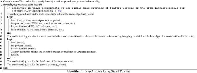
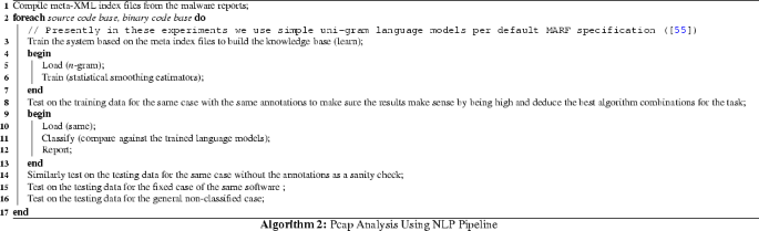
• -binary – treat data as pure binary non-formatted data,

• -nopreprep – to skip extra pre-pre-processing,

• -sdwt – use separating discrete wavelet transform, and

• -flucid – generate Forensic Lucid expressions for subsequent forensic investigations and reasoning in an external system [58].

References

Abdelnour, A.F., Selesnick, I.W.: Nearly symmetric orthogonal wavelet bases. In: Proceedings of the IEEE International Conference on Acoustics, Speech, Signal Processing (ICASSP) (2001a)
Aggarwal, C.C., Gates, S.C., Yu, P.S.: On the merits of building categorization systems by supervised clustering. In: KDD, KDD’99, pp. 352–356. ACM, New York, NY (1999)
Alshammari, R.A., Zincir-Heywood, A.N.: Investigating two different approaches for encrypted traffic classification. In: Proceedings of the Sixth Annual Conference on Privacy, Security and Trust (PST’08), pp. 156–166. IEEE Computer Society, Washington, DC (2008)
Alshammari, R.A., Zincir-Heywood, A.N.: Machine learning based encrypted traffic classification: Identifying SSH and Skype. In: Proceedings of the IEEE Symposium on Computational Intelligence for Security and Defense Applications (CISDA 2009), pp. 1–8. IEEE (2009)
Alshammari, R.A.: Automatically generating robust signatures using a machine learning approach to unveil encrypted VOIP traffic without using port numbers, IP addresses and payload inspection. Ph.D. thesis, Dalhousie University, Halifax, Nova Scotia (2012)
Bailey, M., Oberheide, J., Andersen, J., Mao, Z.M., Jahanian, F., Nazario, J.: Automated classification and analysis of Internet malware. Tech. rep., University of Michigan (2007). http://www.eecs.umich.edu/techreports/cse/2007/CSE-TR-530-07.pdf
Bayer, U., Comparetti, P.M., Hlauschek, C., Kruegel, C., Kirda, E.: Scalable, behavior-based malware clustering. In: NDSS, vol. 9 (2009)
Binkley, J.R., Singh, S.: An algorithm for anomaly-based botnet detection. In: Proceedings of the 2nd conference on Steps to Reducing Unwanted Traffic on the Internet, no. 2 in SRUTI, pp. 1–7. USENIX Association, Berkeley, CA (2006)
Bloedorn, E., Christiansen, A.D., Hill, W., Skorupka, C., Talbot, L.M., Tivel, J.: Data mining for network intrusion detection: How to get started. Tech. rep., The MITRE Corporation (2001). http://citeseerx.ist.psu.edu/viewdoc/download?doi=10.1.1.102.8556&rep=rep1&type=pdf
Boggs, N., Hiremagalore, S., Stavrou, A., Stolfo, S.J.: Cross-domain collaborative anomaly detection: so far yet so close. In: Recent Advances in Intrusion Detection, pp. 142–160. Springer, Berlin (2011)
Boukhtouta, A., Lakhdari, N.E., Mokhov, S.A., Debbabi, M.: Towards fingerprinting malicious traffic. In: Proceedings of ANT’13, vol. 19, pp. 548–555. Elsevier, Amsterdam (2013). doi:10.1016/j.procs.2013.06.073
Bozorgi, M., Saul, L.K., Savage, S., Voelker, G.M.: Beyond heuristics: Learning to classify vulnerabilities and predict exploits. In: Proceedings of the 16th ACM SIGKDD International Conference on Knowledge Discovery and Data Mining, KDD’10, pp. 105–114. ACM, New York, NY (2010). doi:10.1145/1835804.1835821
Chang, S., Daniels, T.E.: P2P botnet detection using behavior clustering & statistical tests. In: Proceedings of the 2nd ACM Workshop on Security and Artificial Intelligence. AISec, pp. 23–30. ACM, New York, NY (2009)
CrySyS Lab: sKyWIper (a.k.a. Flame a.k.a. Flamer): A complex malware for targeted attacks. Tech. rep., Budapest University of Technology and Economics: Department of Telecommunications, Budapest, Hungary (2012). http://www.crysys.hu/skywiper/skywiper.pdf
Dhillon, I.S., Mallela, S., Kumar, R.: A divisive information theoretic feature clustering algorithm for text classification. J. Mach. Learn. Res. 3, 1265–1287 (2003)
Dietrich, C.J., Rossow, C., Pohlmann, N.: CoCoSpot: clustering and recognizing botnet command and control channels using traffic analysis. Comput. Netw. 57(2), 475–486 (2013)
Duda, R.O., Hart, P.E., Stork, D.G.: Pattern Classification. Wiley, New York (2012)
Fan, W., Miller, M., Stolfo, S., Lee, W., Chan, P.: Using artificial anomalies to detect unknown and known network intrusions. In: Proceedings of the IEEE International Conference on Data Mining (ICDM 2001), pp. 123–130 (2001). doi:10.1109/ICDM.2001.989509
Frank, E.: J48. [online] (2012). http://weka.sourceforge.net/doc.dev/weka/classifiers/trees/J48.html
Frank, E., Legg, S., Inglis, S.: Class SMO. [online] (2012). http://weka.sourceforge.net/doc/weka/classifiers/functions/SMO.html
Freund, Y.: Boosting a weak learning algorithm by majority. Inf. Comput. 121(2), 256–285 (1995)
Golovko, V., Bezobrazov, S., Kachurka, P., Vaitsekhovich, L.: Neural network and artificial immune systems for malware and network intrusion detection. In: Advances in Machine Learning II, pp. 485–513. Springer, Berlin (2010)
Gu, G., Porras, P., Yegneswaran, V., Fong, M., Lee, W.: BotHunter: detecting malware infection through IDS-driven dialog correlation. In: Proceedings of 16th USENIX Security Symposium, SS, pp. 1–16. USENIX Association, Berkeley, CA (2007)
Gu, G., Zhang, J., Lee, W.: BotSniffer: Detecting botnet command and control channels in network traffic. In: Proceedings of the Network and Distributed System Security Symposium, NDSS. The Internet Society (2008)
Gu, G., Perdisci, R., Zhang, J., Lee, W.: BotMiner: clustering analysis of network traffic for protocol- and structure-independent botnet detection. In: Proceedings of the 17th Security Symposium, SS, pp. 139–154. USENIX Association, Berkeley, CA (2008)
Han, B.: Towards a multi-tier runtime system for GIPSY. Master’s thesis, Department of Computer Science and Software Engineering, Concordia University, Montreal (2010)
Han, J.: Data Mining: Concepts and Techniques. Morgan Kaufmann Publishers Inc., San Francisco, CA (2005)
Hearst, M.A., Dumais, S., Osman, E., Platt, J., Scholkopf, B.: Support vector machines. IEEE of Intelligent Systems and Their Applications 13(4), 18–28 (1998)
Hu, X., Shin, K.G., Bhatkar, S., Griffin, K.: MutantX-S: Scalable malware clustering based on static features. In: USENIX Annual Technical Conference, pp. 187–198 (2013)
Ji, Y.: Scalability evaluation of the GIPSY runtime system. Master’s thesis, Department of Computer Science and Software Engineering, Concordia University, Montreal (2011). http://spectrum.library.concordia.ca/7152/
Karasaridis, A., Rexroad, B., Hoeflin, D.: Wide-scale botnet detection and characterization. In: Proceedings of the First Workshop on Hot Topics in Understanding Botnets, HotBots, pp. 1–7. USENIX Association, Berkeley, CA (2007)
Karypis Lab: Data clustering software. [online] (2006–2014). http://glaros.dtc.umn.edu/gkhome/views/cluto
Katz, G., Shabtai, A., Rokach, L., Ofek, N.: ConfDTree: Improving decision trees using confidence intervals. In: 12th IEEE International Conference on, Data Mining (ICDM), pp. 339–348 (2012)
Kheir, N., Blanc, G., Debar, H., Garcia-Alfaro, J., Yang, D.: Automated classification of C&C connections through malware URL clustering. In: ICT Systems Security and Privacy Protection, pp. 252–266. Springer, Berlin (2015)
Kirat, D., Nataraj, L., Vigna, G., Manjunath, B.S.: SigMal: a static signal processing based malware triage. In: ACSAC’13. ACM, New York, NY (2013). doi:10.1145/2523649.2523682
Kokare, M., Biswas, P.K., Chatterji, B.N.: Texture image retrieval using new rotated complex wavelet filters. IEEE Transaction on Systems, Man, and Cybernetics-Part B: Cybernetics 6(35), 1168–1178 (2005)
Kokare, M., Biswas, P.K., Chatterji, B.N.: Rotation-invariant texture image retrieval using rotated complex wavelet filters. IEEE Transaction on Systems, Man, and Cybernetics-Part B: Cybernetics 6(36), 1273–1282 (2006)
Kremenek, T., Engler, D.: Z-ranking: Using statistical analysis to counter the impact of static analysis approximations. In: SAS 2003 (2003)
Kremenek, T., Ashcraft, K., Yang, J., Engler, D.: Correlation exploitation in error ranking. In: Foundations of Software Engineering (FSE) (2004)
Kremenek, T., Twohey, P., Back, G., Ng, A., Engler, D.: From uncertainty to belief: inferring the specification within. In: Proceedings of the 7th Symposium on Operating System Design and Implementation (2006)
Larsen, B., Aone, C.: Fast and effective text mining using linear-time document clustering. In: KDD, KDD’99, pp. 16–22. ACM, New York, NY (1999)
Lee, W.: Applying data mining to intrusion detection: the quest for automation, efficiency, and credibility. ACM SIGKDD Explorations Newsletter 4(2), 35–42 (2001)
Lee, W., Stolfo, S.J., Mok, K.W.: Adaptive intrusion detection: a data mining approach. Artificial Intelligence Review 14, 533–567 (2000). doi:10.1023/1006624031083
Li, R., Xi, O.J., Pang, B., Shen, J., Ren, C.L.: Network application identification based on wavelet transform and k-means algorithm. In: Proceedings of the IEEE International Conference on Intelligent Computing and Intelligent Systems (ICIS2009), vol. 1, pp. 38–41 (2009). doi:10.1109/ICICISYS.2009.5357939
Li, W., Canini, M., Moore, A.W., Bolla, R.: Efficient application identification and the temporal and spatial stability of classification schema. Comput. Netw. 53, 790–809 (2009)
Limthong, K., Kensuke, F., Watanapongse, P.: Wavelet-based unwanted traffic time series analysis. In: 2008 International Conference on Computer and Electrical Engineering, pp. 445–449. IEEE Computer Society, Washington, DC (2008). doi:10.1109/ICCEE.2008.106
Livadas, C., Walsh, R., Lapsley, D.E., Strayer, W.T.: Using machine learning techniques to identify botnet traffic. In: LCN, pp. 967–974. IEEE Computer Society, Washington, DC (2006)
Locasto, M.E., Parekh, J.J., Stolfo, S., Misra, V.: Collaborative distributed intrusion detection. Tech. Rep. CUCS-012-04 (2004). http://hdl.handle.net/10022/AC:P:29215
Locasto, M.E., Parekh, J.J., Keromytis, A.D., Stolfo, S.J.: Towards collaborative security and P2P intrusion detection. In: Proceedings of the Information Assurance Workshop (IAW’05), from the Sixth Annual IEEE SMC, pp. 333–339. IEEE (2005)
Manning, C.D., Schutze, H.: Foundations of Statistical Natural Language Processing. MIT Press, Cambridge, MA (2002)
MathWorks: MATLAB. [online] (2000–2012). http://www.mathworks.com/products/matlab/
MathWorks: MATLAB Coder. [online] (2012). http://www.mathworks.com/help/toolbox/coder/coder_product_page.html, last viewed June 2012
MathWorks: MATLAB Coder: codegen—generate C/C++ code from MATLAB code. [online] (2012). http://www.mathworks.com/help/toolbox/coder/ref/codegen.html, last viewed June 2012
McLachlan, G., Krishnan, T.: The EM Algorithm and Extensions, vol. 382. Wiley, New York (2007)
Mokhov, S.A.: Study of best algorithm combinations for speech processing tasks in machine learning using median vs. mean clusters in MARF. In: Desai, B.C. (ed.) Proceedings of C3S2E’08, pp. 29–43. ACM, Montreal, Quebec (2008). doi:10.1145/1370256.1370262
Mokhov, S.A.: MARFCAT—MARF-based Code Analysis Tool. Published electronically within the MARF project. http://sourceforge.net/projects/marf/files/Applications/MARFCAT/ (2010–2015). Last viewed February 2014
Mokhov, S.A.: The use of machine learning with signal- and NLP processing of source code to fingerprint, detect, and classify vulnerabilities and weaknesses with MARFCAT. Tech. Rep. NIST SP 500–283, NIST (2011). Report: http://www.nist.gov/manuscript-publication-search.cfm?pub_id=909407, online e-print at http://arxiv.org/abs/1010.2511
Mokhov, S.A.: Intensional cyberforensics. Ph.D. thesis, Department of Computer Science and Software Engineering, Concordia University, Montreal (2013). arXiv:1312.0466
Mokhov, S.A., Debbabi, M.: File type analysis using signal processing techniques and machine learning vs. file unix utility for forensic analysis. In: O. Goebel, S. Frings, D. Guenther, J. Nedon, D. Schadt (eds.) Proceedings of the IT Incident Management and IT Forensics (IMF’08), LNI140, pp. 73–85. GI (2008)
Mokhov, S.A., Paquet, J., Debbabi, M.: Formally specifying operational semantics and language constructs of Forensic Lucid. In: O. Göbel, S. Frings, D. Günther, J. Nedon, D. Schadt (eds.) Proceedings of the IT Incident Management and IT Forensics (IMF’08), LNI, vol. 140, pp. 197–216. GI (2008). Online at http://subs.emis.de/LNI/Proceedings/Proceedings140/gi-proc-140-014.pdf
Mokhov, S.A., Paquet, J., Debbabi, M.: Towards automatic deduction and event reconstruction using Forensic Lucid and probabilities to encode the IDS evidence. In: S. Jha, R. Sommer, C. Kreibich (eds.) Proceedings of Recent Advances in Intrusion Detection RAID’10, Lecture Notes in Computer Science (LNCS), vol. 6307, pp. 508–509. Springer, Berlin (2010). doi:10.1007/978-3-642-15512-3_36
Mokhov, S.A., Paquet, J., Debbabi, M.: The use of NLP techniques in static code analysis to detect weaknesses and vulnerabilities. In: M. Sokolova, P. van Beek (eds.) Proceedings of Canadian Conference on AI’14, LNAI, vol. 8436, pp. 326–332. Springer, Berlin (2014). doi:10.1007/978-3-319-06483-3_33. Short paper
Mokhov, S.A., Paquet, J., Debbabi, M.: MARFCAT: Fast code analysis for defects and vulnerabilities. In: Proceedings of SWAN’15, pp. 35–38. IEEE (2015) (to appear)
Motorola: Efficient polyphase FIR resampler for numpy: Native C/C++ implementation of the function upfirdn(). [online] (2009). http://code.google.com/p/upfirdn/source/browse/upfirdn
Murphy, K.P.: HMM toolbox. [online] (2002–2014). http://www.cs.ubc.ca/murphyk/Software/HMM/hmm_download.html
Nari, S., Ghorbani, A.A.: Automated malware classification based on network behavior. In: Proceedings of the 2013 International Conference on Computing, Networking and Communications (ICNC), pp. 642–647. IEEE (2013)
Noh, S.K., Oh, J.H., Lee, J.S., Noh, B.N., Jeong, H.C.: Detecting p2p botnets using a multi-phased flow model. In: International Conference on Digital Society, ICDS, pp. 247–253. IEEE Computer Society, Washington, DC (2009)
Okada, Y., Ata, S., Nakamura, N., Nakahira, Y., Oka, I.: Comparisons of machine learning algorithms for application identification of encrypted traffic. In: Proceedings of the 10th International Conference on Machine Learning and Applications and Workshops (ICMLA), vol. 2, pp. 358–361 (2011)
Okun, V., Delaitre, A., Black, P.E., NIST SAMATE: Static Analysis Tool Exposition (SATE) 2010. [online] (2010). http://samate.nist.gov/SATE2010Workshop.html
Ouchani, S., Ait’Mohamed, O., Debbabi, M.: A non-convex classifier support for abstraction-refinement framework. In: 24th International Conference on Microelectronics (ICM), pp. 1–4 (2012)
Paquet, J.: Distributed eductive execution of hybrid intensional programs. In: Proceedings of the 33rd Annual IEEE International Computer Software and Applications Conference (COMPSAC’09), pp. 218–224. IEEE Computer Society, Washington, DC (2009). doi:10.1109/COMPSAC.2009.137
Paxson, V.: Bro: a system for detecting network intruders in real-time. Comput. Netw. 31(23–24), 2435–2463 (1999). http://www.icir.org/vern/papers/bro-CN99.pdf
Peng, Y., Kou, G., Sabatka, A., Chen, Z., Khazanchi, D., Shi, Y.: Application of clustering methods to health insurance fraud detection. In: Proceedings of the 2006 International Conference on Service Systems and Service Management, vol. 1, pp. 116–120 (2006)
Perdisci, R., Ariu, D., Fogla, P., Giacinto, G., Lee, W.: McPAD: a multiple classifier system for accurate payload-based anomaly detection. Comput. Netw. 53(6), 864–881 (2009)
Quinlan, R.: C4.5: Programs for Machine Learning. Morgan Kaufmann Publishers, San Mateo, CA (1993)
Rahimian, A., Ziarati, R., Preda, S., Debbabi, M.: On the reverse engineering of the Citadel botnet. In: Foundations and Practice of Security. Lecture Notes in Computer Science, pp. 408–425. Springer, Berlin (2014)
Rieck, K., Holz, T., Willems, C., Düssel, P., Laskov, P.: Learning and classification of malware behavior. In: Detection of Intrusions and Malware, and Vulnerability Assessment, pp. 108–125. Springer, Berlin (2008)
Rodríguez, L.J., Torres, I.: Comparative study of the baum-welch and viterbi training algorithms applied to read and spontaneous speech recognition. In: Pattern Recognition and Image Analysis. Lecture Notes in Computer Science, vol. 2652, pp. 847–857. Springer, Berlin (2003)
Rossow, C., Dietrich, C.J., Bos, H., Cavallaro, L., Van Steen, M., Freiling, F.C., Pohlmann, N.: Sandnet: network traffic analysis of malicious software. In: Proceedings of the First Workshop on Building Analysis Datasets and Gathering Experience Returns for Security, pp. 78–88. ACM, New york (2011)
Salton, G.: Automatic Text Processing: The Transformation, Analysis, and Retrieval of Information by Computer. Addison-Wesley, Boston, MA (1989)
Schreiber, R.: MATLAB. Scholarpedia 2(6), 2929 (2007). doi:10.4249/scholarpedia.2929. http://www.scholarpedia.org/article/MATLAB
Schultz, M.G., Eskin, E., Zadok, E., Stolfo, S.J.: Data mining methods for detection of new malicious executables. In: Proceedings of IEEE Symposium on Security and Privacy, pp. 38–49. Oakland (2001)
Selesnick, I., Cai, S., Li, K., Sendur, L., Abdelnour, A.F.: MATLAB implementation of wavelet transforms. Tech. rep., Electrical Engineering, Polytechnic University, Brooklyn, NY (2003). http://taco.poly.edu/WaveletSoftware/
Simon, G.J., Xiong, H., Eilertson, E., Kumar, V.: Scan detection: a data mining approach. In: Proceedings of SDM 2006, pp. 118–129. SIAM, Philadelphia, PA (2006). http://www.siam.org/meetings/sdm06/proceedings/011simong.pdf
Sly Technologies Inc: jNetPcap OpenSource. [online] (2012). http://www.jnetpcap.com/
Song, D.: BitBlaze: Security via binary analysis. [online] (2010). http://bitblaze.cs.berkeley.edu
Song, D.: WebBlaze: New techniques and tools for web security. [online] (2010). http://webblaze.cs.berkeley.edu
Song, Y., Keromytis, A.D., Stolfo, S.: Spectrogram: a mixture-of-markov-chains model for anomaly detection in web traffic. In: Proceedings of the Network and Distributed System Security Symposium, pp. 121–135. Internet Society (2009)
Sourcefire: Snort: open-source network intrusion prevention and detection system (IDS/IPS). [online] (1999–2015). http://www.snort.org/
Stolfo, S.J., Lee, W., Chan, P.K., Fan, W., Eskin, E.: Data mining-based intrusion detectors: an overview of the Columbia IDS Project. ACM SIGMOD Record 30(4), 5–14 (2001)
Su, J., Zhang, H.: A fast decision tree learning algorithm. In: Proceedings of the 21st National Conference on Artificial Intelligence, AAAI’06, vol. 1, pp. 500–505. AAAI Press (2006)
Tegeler, F., Fu, X., Vigna, G., Kruegel, C.: BotFinder: finding bots in network traffic without deep packet inspection. In: Proceedings of the 8th International Conference on Emerging Networking Experiments and Technologies, CoNEXT, pp. 349–360. ACM, New York, NY (2012)
The Weka Project: Weka 3: data mining with open source machine learning software in Java. [online] (2006–2014). http://www.cs.waikato.ac.nz/ml/weka/
Thorat, S.A., Khandelwal, A.K., Bruhadeshwar, B., Kishore, K.: Payload content based network anomaly detection. In: Proceedings of the First International Conference on the Applications of Digital Information and Web Technologies (ICADIWT 2008), pp. 127–132. IEEE (2008)
ThreatTrack Security: ThreadAnalyzer: dynamic sandboxing and malware analysis (formerly GFI SandBox). [online] (2013). http://www.threattracksecurity.com/enterprise-security/sandbox-software.aspx
Trinius, P., Willems, C., Holz, T., Rieck, K.: A malware instruction set for behavior-based analysis (2011)
Vassev, E.I.: General architecture for demand migration in the GIPSY demand-driven execution engine. Master’s thesis, Department of Computer Science and Software Engineering, Concordia University, Montreal (2005). http://spectrum.library.concordia.ca/8681/
Wang, K., Stolfo, S.J.: Anomalous payload-based network intrusion detection. In: Recent Advances in Intrusion Detection, pp. 203–222. Springer, Berlin (2004)
Whalen, S., Boggs, N., Stolfo, S.J.: Model aggregation for distributed content anomaly detection. In: Proceedings of the 2014 Workshop on Artificial Intelligent and Security Workshop, pp. 61–71. ACM, New York (2014)
Wicherski, G.: pehash: a novel approach to fast malware clustering. In: 2nd USENIX Workshop on Large-Scale Exploits and Emergent Threats (LEET) (2009)
Wireless and Secure Networks Research Lab: WISNET: downloads. [online] (2009–2014). http://wisnet.seecs.nust.edu.pk/downloads.php
Wu, M.D., Wolfthusen, S.D.: Network forensics of partial SSL/TLS encrypted traffic classification using clustering algorithms. In: O. Göbel, S. Frings, D. Günther, J. Nedon, D. Schadt (eds.) Proceedings of the IT Incident Management and IT Forensics (IMF’08), LNI140, pp. 157–172 (2008)
Yen, T.F., Reiter, M.K.: Traffic aggregation for malware detection. In: Proceedings of the 5th international conference on Detection of Intrusions and Malware, and Vulnerability Assessment, DIMVA, pp. 207–227. Springer, Berlin (2008)
Zanero, S.: Analyzing TCP traffic patterns using self organizing maps. In: Image Analysis and Processing (ICIAP 2005), pp. 83–90. Springer, Berlin (2005)
Zanero, S., Savaresi, S.M.: Unsupervised learning techniques for an intrusion detection system. In: Proceedings of the 2004 ACM Symposium on Applied Computing, pp. 412–419. ACM, New York (2004)
Zanero, S., Serazzi, G.: Unsupervised learning algorithms for intrusion detection. In: Network Operations and Management Symposium (NOMS 2008), pp. 1043–1048. IEEE (2008)
Zetter, K.: Meet ‘Flame’, The Massive Spy Malware Infiltrating Iranian Computers. WIRED (2012). http://www.wired.com/threatlevel/2012/05/flame/
Zhang, D., Liu, D., Csallner, C., Kung, D., Lei, Y.: A distributed framework for demand-driven software vulnerability detection. J. Syst. Softw. 87, 60–73 (2014). doi:10.1016/j.jss.2013.08.033
Zhao, Y., Karypis, G.: Criterion functions for document clustering: experiments and analysis. Tech. rep., University of Minnesota (2002)
Zhao, Y., Karypis, G., Fayyad, U.: Hierarchical clustering algorithms for document datasets. Data Min. Knowl. Discov. 10(2), 141–168 (2005)
Zhong, S., Ghosh, J.: Generative model-based document clustering: a comparative study. Knowl. Inf. Syst. 8(3), 374–384 (2005)
Author information
Authors and Affiliations
Corresponding author