
Abstract
Purpose
In the past decade, several methods have emerged to quantify water scarcity, water availability and the human health impacts of water use. It was recommended that a quantitative comparison of methods should be performed to describe similar impact pathways, namely water scarcity and human health impacts from water deprivation. This is precisely the goal of this paper, which aims to (1) identify the key relevant modeling choices that explain the main differences between characterization models leading to the same impact indicators; (2) quantify the significance of the differences between methods, and (3) discuss the main methodological choices in order to guide method development and harmonization efforts.
Methods
The modeling choices are analysed for similarity of results (using mean relative difference) and model response consistency (through rank correlation coefficient). Uncertainty data associated with the choice of model are provided for each of the models analysed, and an average value is provided as a tool for sensitivity analyses.
Results
The results determined the modeling choices that significantly influence the indicators and should be further analysed and harmonised, such as the regional scale at which the scarcity indicator is calculated, the sources of underlying input data and the function adopted to describe the relationship between modeled scarcity indicators and the original withdrawal-to-availability or consumption-to-availability ratios. The inclusion or exclusion of impacts from domestic user deprivation and the inclusion or exclusion of trade effects both strongly influence human health impacts. At both midpoint and endpoint, the comparison showed that considering reduced water availability due to degradation in water quality, in addition to a reduction in water quantity, greatly influences results. Other choices are less significant in most regions of the world. Maps are provided to identify the regions in which such choices are relevant.
Conclusions
This paper provides useful insights to better understand scarcity, availability and human health impact models for water use and identifies the key relevant modeling choices and differences, making it possible to quantify model uncertainty and the significance of these choices in a specific regional context. Maps of regions where these specific choices are of importance were generated to guide practitioners in identifying locations for sensitivity analyses in water footprint studies. Finally, deconstructing the existing models and highlighting the differences and similarities has helped to determine building blocks to support the development of a consensual method.
1 Introduction
This paper is divided into two parts and aims to broaden the understanding of existing water use impact assessment methods and their applicability within a water footprint study. Part A focuses on identifying relevant modeling choices to analyse the main differences between water impact assessment methods and assess their overall variability and model uncertainty. Part B illustrates the applicability of water footprint methods through a case study and discusses the methods’ consistency, reliability and limitations for decision making. Sensitivity analyses on the case study were selected based on relevant modeling choices determined in part A.
1.1 Purpose
In LCA, potential impacts from water pollution were traditionally captured by impact categories such as (eco)toxicity, acidification and eutrophication. The impacts of using the resource itself (impacts of water use) and reducing the availability of water for other users—humans and ecosystems—were not yet captured until recently. Since the preliminary discussion on the topic began in the early 2000s (Owens 2002; Bauer and Zapp 2005; Brent 2004), several methods have emerged and entirely or partially address the different impact pathways outlined in the general framework proposed by Bayart et al. (2010). Kounina et al. (2013) (see Electronic Supplementary Material, Fig. S1) reviewed and analysed the developed methods and their scopes, strengths and weaknesses. At the midpoint level, most existing methods quantify water scarcity based on a use-to-availability ratio, referred to as scarcity or stress index. At the damage level, impacts are generally modeled up to specific endpoints within a given area of protection: human health, ecosystem quality or resources.
The review showed that existing methods sometimes model complementary impact pathways or the exact same ones based on different modeling approaches and assumptions. Building on Kounina et al.’s (2013) review, this paper aims to: (1) identify the key relevant modeling choices that explain the main differences between characterisation models leading to the same impact indicators (scarcity, availability and human health); (2) quantify the significance of the differences between methods, and (3) discuss the main methodological choices in order to guide method development and harmonisation efforts. The goal of this paper is not to provide recommendation regarding the use of one method over another. This paper constitutes the third deliverable of the UNEP/SETAC Life Cycle Initiative Working Group on Water Use in LCAA and represents a stepping stone towards its goal to develop a harmonised method through scientific consensus on existing methods (Life Cycle Initiative 2012).
1.2 Presentation of methods analysed
The methods chosen for this comparison focus on human health, with scarcity as an intermediate indicator along the impact pathway. Figure 1 provides a detailed description of the selected methods along the impact pathways leading to human health. A summary table of the methods and their associated names is presented in the Electronic Supplementary Material, Table S1. Damage-oriented methods assessing impacts on ecosystems address impact pathways that are considered complementary (Kounina et al. 2013) and are therefore excluded from the scope of the comparison. The resource depletion damage category is still under debate and not yet mature enough to be included in the scope of this paper.

Description of method-specific impact pathways leading to potential impact to human health. Choices made related to the inventory and in the modeling of the parameters (blue boxes) are analysed
1.2.1 Midpoint: scarcity and availability
The scarcity and availability methods reviewed by Kounina et al. (2013) are selected for the model comparison, except for Ridoutt and Pfister (2010). The latter was excluded because the authors suggest using a different approach (Ridoutt and Pfister 2013). In this paper, and as a proposal for future consistency, scarcity refers to the pressure on the resource from a quantity perspective only, and availability refers to an assessment of lower water availability due to water quality degradation and quantity depletion. This is in line with the terminology used in the International Standards Organisation (ISO) standard on Water Footprint 14046 (ISO 14046 2014).
-
Swiss Ecoscarcity (named M-SwissSc) (Frischknecht et al. 2008)
The Swiss ecological scarcity method is based on the distance-to-target principle, which is similar to using a withdrawal-to-availability (WTA) ratio based scarcity indicator. All withdrawn volumes in a region are considered and divided by the critical water use volume for this region with data from WaterGap (Alcamo et al. 2003a) (in the updated version). The critical volume is defined as the fraction of water use at which scarcity begins to occur, set by default to 20 % of the renewable water available. This fraction is then squared and normalised using a reference region (the default is Switzerland). Results are given in eco-points (scaled by a constant to obtain readily presentable numerical quantities) at the country and grid-cell levels (0.5° × 0.5°). The indicator is applied to the volume of water that is consumed or withdrawn and therefore assesses consumptive water use or all water use reported in ecoinvent 2, except for hydropower production.
-
Pfister WSI (named M-PfisterSc) (Pfister et al. 2009)
This scarcity indicator is based on a WTA ratio, modified to account for seasonal variations, and modeled using a logistic function (S-curve) in order to obtain resulting indicator values between 0.01 and 1 m3 deprived/m3 consumed. The curve is tuned using OCDE water scarcity (stress) thresholds, which define moderate and severe water stress as 20 and 40 % of withdrawals, respectively (Alcamo et al. 2000). The model is available at the grid-cell level (0.5° × 0.5°), and data for water withdrawals and availability were obtained from the WaterGap model (Alcamo et al. 2003b). The indicator is applied to the consumed water volume (i.e. assesses consumptive water use only).
-
Blue water scarcity (named M-BWSc) (Hoekstra et al. 2012)
This scarcity indicator is based on a consumption-to-availability ratio (CTA) calculated as the fraction between consumed (referred to as blue water footprint) and available water. The latter considers all runoff water, of which 80 % is subtracted to account for environmental water needs. The data are from Fekete et al.(2002) for water runoff and Mekonnen and Hoekstra (2011) for water consumption. Results are available for the main watersheds worldwide, but many outlying regions are not covered. The indicator is applied to the consumed water volume (i.e. assesses consumptive water use only).
-
Boulay—simplified methodology considering consumptive use only (named M-BoulaySc) (Boulay et al. 2011b)
This scarcity indicator is based on a CTA ratio (using statistical low-flow to account for seasonal variations) and modeled using a logistic function (S-curve) in order to obtain resulting indicator values between 0 and 1 m3 deprived/m3 consumed. The curve is tuned using the same water scarcity thresholds as the OECD thresholds in M-PfisterSc (Alcamo et al. 2000) but converted with an empirical correlation between WTA and CTA. More specific scarcity indicators are also available for surface and groundwater based on the same approach as for water from unspecified origin. Water consumption and availability data for surface and ground water are taken from the WaterGap 2.2 model (grid cell level). Results are available at a scale that originates from the intersection of the watershed and country scales, resulting in 808 cells worldwide. The simplified method does not consider changes in water quality, unlike the original one (presented in the next paragraph). The indicator is applied to the consumed water volume (i.e. assesses consumptive water use only).
-
Boulay—original method, including quality aspects (named M-BoulayAv) (Boulay et al. 2011b)
This availability indicator assesses degradative and consumptive water use. The same characterisation model as M-BoulaySc is used, though it is differentiated for eight water categories that each correspond to an inventory flow that describes a type of water (surface or groundwater) of a given quality that is acceptable for specific human uses (domestic, etc.). This indicator assesses degradative and consumptive water use by characterising input and output flows of water from a process and their difference in quantity and quality. Default values on local availability and water quality are taken from the GEMStat database (UNEP Global Environment Monitoring System (GEMS) Water Programme 2009).
-
Veolia Water Impact Index (named M-WIIXAv) (Bayart et al. 2014)
The impact index is calculated as the product of (1) a water scarcity indicator (M-PfisterSc) and (2) a quality indicator, hence categorised as an availability method. The quality indicator is calculated as a ratio between a reference concentration—based on environmental quality standards (EQS) targeted to protect the receiving water bodies—and the actual concentration of the inventory flows. Since EQS are pollutant-specific, the quality index is driven by the most penalizing ratio. It is set to a maximum of 1 when the concentration of the inventory flow is below the reference concentration for all pollutants, meaning that the impact of consuming EQS-compliant water yields maximum impacts whereas consuming non-EQS-compliant water for at least one contaminant has fewer impacts (the higher the index, the greater the impacts). This indicator assesses degradative and consumptive water uses by characterising the input and output flows of water in a process.
1.2.2 Endpoint impacts on human health
So far, the human health impacts of water deprivation have been modeled using four parameters: 1 scarcity (how much of the water used will deprive other users?); 2 distribution of affected users (which users will be deprived by which fraction of unavailable water?); 3 socio-economic parameter (to what extent will the deprived users suffer health impacts and remain unable to adapt through economic resources?) and 4 effect factor (what is the effect on human health of a specific user being deprived of a certain amount of water?). Equation 1 (Aguilar-Manjarrez 2006) represents how these parameters interact in a generic model. Pfister (Pfister et al. 2009) and Boulay (Boulay et al. 2011b) model each parameter explicitly, whereas Motoshita_dom (Motoshita et al. 2010b) uses a statistical regression that merges steps 3 and 4 into a single modeling step (see Fig. 1). The intermediary parameters express different modeling components along the cause effect chain (see Fig. 1) and are kept distinct to gain insight into their individual contributions to the total results. Characterisation models and factors assessing the impacts of depriving domestic users, agricultural users and/or fisheries of sufficient water are analysed individually, since the pathways can lead to different direct human health endpoints expressed in DALY (disability-adjusted life years).
Where:
- CFi :
-
Characterisation factor describing the potential human health impacts of water deprivation of user i (agriculture, domestic user or fisheries)
- SI:
-
Scarcity or availability index, depending on the inclusion (availability) or exclusion (scarcity) of quality in the index
- DAUi :
-
Distribution of affected users i (i.e. fraction of water use that affects user i)
- SEP:
-
Socio-economic parameter
- EFi :
-
Effect factor for water deprivation of user i
- SEEi factor:
-
Socio-economic and effect factor
-
Pfister (named E-Pfister)(Pfister et al. 2009)
This endpoint indicator expressed in DALY is obtained by modeling the cause–effect chain of water deprivation for agricultural users (lack of irrigation water) leading to malnutrition. It assumes that there is no general causality from water consumption to lack of water for domestic use, arguing that water access for domestic use is mainly dependent on infrastructure (and not on water) availability. It builds on the scarcity indicator (M-PfisterSc) and models the cause–effect chain by multiplying it by (1) the agricultural users’ share of water use (as DAU) from Vörösmarty (Vorosmarty et al. 2000)), (2) a socio-economic parameter defined as a human development factor for malnutrition, which relates the Human Development Index (a composite index representing human development by considering life expectancy, education and income published by the UNDP) to malnutrition vulnerability and (3) two values independent of location combined in an effect factor that describes the DALY/m3 of water deprived for agriculture: the per-capita water requirements to prevent malnutrition (in cubic meters/(year•capita)) and the damage factor denoting the damage caused by malnutrition (DALY/(year•capita)). The effect factor therefore carries two underlying assumptions: (1) global malnutrition health impacts are exclusively caused by a lack of water for irrigation, and (2) a case of malnutrition occurs only once all the water required for one person is no longer available. The first assumption may lead to an overestimation of impacts while the second may lead to an underestimation. The results are derived on a 0.5° × 0.5° grid cell scale and aggregated at the watershed level (>10,000 watersheds, as in (Alcamo et al. 2003a).
-
Boulay (named E-Boulay with different variants: _agri, _dom, _marg, _distri, _Q) (Boulay et al. 2011b)
This endpoint indicator expressed in DALY is obtained by modeling each water user’s loss of functionality. It addresses three different impact pathways: malnutrition from water deprivation for agricultural users, malnutrition from water deprivation for fisheries and water-related diseases associated with a lack of water for domestic use. Four model scenarios are considered by E-Boulay as a cross-combination of both original versions (addressing consumption and degradation with suffix _Q) and the simplified version (which only addresses consumption) of the model and two key modeling hypotheses: distribution and marginal. Distribution (Boulay_distri or Boulay_distri_Q) refers to the impact assessment in which all users are competing and proportionally affected according to their distributional share of water use for off-stream users (here, agriculture and domestic). Marginal (E-Boulay_marg or E-Boulay_marg_Q) refers to a modeling choice in which an additional water use will deprive only one off-stream user (in addition to in-stream users here, fisheries). The one for which water has less value was set as agriculture by default. This hypothesis therefore excludes potential impacts to domestic users. The distribution among users from WaterGap is used to determine the distribution of affected users for Boulay_distri (factor giving the cubic meter deprived distribution between affected users). The socio-economic parameter used in all E_Boulay methods is one minus the adaptation capacity (AC). High-income countries are considered to fully adapt (AC = 1) whereas low-income countries are considered not to adapt at all (AC = 0) to water deprivation. The adaptation capacity of medium-income countries is considered to be linearly correlated with gross national income (GNI) per capita. The effect factor uses country-specific statistical data to obtain the relationship between health impacts from malnutrition (DALY/kcal of malnutrition × kilocalorie produced per cubic meter for agricultural use or kilocalorie produced per cubic meter for aquaculture use), associating 50 % of malnutrition health impacts to a lack of calorie intake and the remaining 50 % to water-related diseases, since they often lead to malnutrition. These 50 % are added to the health impacts in DALY from water-related diseases and divided by the amount of water lacking for domestic use based on the minimum requirement of 50 L/cap/day and the actual regional water use by domestic users, resulting in DALY per cubic meter deprived for domestic use. For both effect factors, a linear relationship is therefore assumed between the health impact and the deprived water. The results are presented according to the M-Boulay spatial scale of from the overlap of the country and main watershed scales for the simplified alternative versions (E-Boulay_distri and E-Boulay_marg) and original methods (E-Boulay_distri_Q and E-Boulay_marg_Q). In this paper, for several analyses, the aggregated characterisation factors (CFs) are separated into domestic and agricultural deprivation parts and referred to as E-Boulay_dom and E-Boulay_agri, respectively.
-
Motoshita (named E-Motoshita with different variants:_dom, _agri, _agri (no TE))
This damage assessment model is based on the sum of two distinct models: one for infectious disease damage caused by domestic water scarcity (Motoshita et al. 2010b) (E-Motoshita_dom) and one for malnutrition damage caused by agricultural water scarcity (Motoshita et al. 2010a) (E-Motoshita_agri).
For domestic water scarcity, the method assumes that water resource scarcity caused by water consumption will lead to a loss of access to safe water. Subsequently, based on location, drinking unsafe water will result in the use of infectious sources and health impairment by disease. The method provides country-based CFs expressed in DALY per cubic meter of water consumed obtained with M-PfisterSc as a scarcity assessment, multiplied by the share of water used by domestic users (from Aquastat) and a combined socio-economic and effect factor obtained by applying non-linear multiple regression analysis considering related socio-economic factors such as GDP, expenditure for capital formation, average temperature, sanitary facilities, nutritional conditions and health expenditure based on statistical data. The factor represents the inaccessibility to safe water due to domestic water scarcity and a subsequent increase in infectious diseases (intestinal nematode infection and diarrhea).
The impacts of malnutrition caused by agricultural water deficit are modeled using the same data source for scarcity and distribution as above, multiplied by a socio-economic parameter describing the trade effect. This illustrates how food supply shortage in a country will spread to other countries through international food trade. It applies a food shortage sharing model based on the proportion of world net import amount (in kilocalories) for net food importer countries that are not able to adapt (or only partially able to adapt) using the adaptation capacity defined in Boulay et al. (2011b) based on GNI. For example, if 1,000 kcal of food are not produced in Spain due to water shortage and local crop productivity, the amount will be distributed among all the world’s net importer countries proportionally to the amount they import (in kilocalories). Countries with low and middle incomes will be affected by the food shortage. This effect is quantified in DALY by using malnutrition-related DALYs in the importing countries (DALYs per kilocalorie malnutrition). The method provides country-based characterisation factors in the context of both domestic and agricultural water scarcity, expressed in DALY per cubic meter of water consumed. The method can also be used without the trade model (E-Motoshita_agri (noTE)) to compare local effects.
2 Methods
The following section describes how the analysis was performed. It is divided into three parts: comparison, analysis of modeling choice and uncertainty assessment. The comparison first assesses how the model results compare at the characterisation factor level and the respective intermediary parameters (identified by the blue squares in Fig. 1). A set of modeling choices was identified, and their sensitivity in terms of the final results was analysed using two versions of the same model, differing only by the option being analysed (e.g. the use of one or another source of data for modeling). For each model, the uncertainty assessment quantifies the uncertainty associated with the choice of model only.
Two statistical indicators were used to compare the models. The difference between the model responses was assessed through the mean difference coefficient (MDC), and the consistency of model response through the rank correlation coefficient (RCC), which are defined below. The correlation coefficient (Pearson’s) was not considered an appropriate indicator because the data revealed heteroscedasticity (i.e. the difference between the values given by two methods is not independent on the value itself). When the homoscedasticity assumption is violated, Pearson’s coefficient of correlation may overestimate the goodness of fit.
The comparison sought to analyse the degree of model response agreement and consistency from one model to the next, rather than their correlation. Two models can have 100 % correlation but may still disagree. A mean relative coefficient (MDC), as described in Eq. 2, was used to represent the difference between two models. It illustrates a mean relative difference, which is the mean of the absolute differences between each data pair divided by their average. It measures dispersion, just like the standard deviation would, but it is not defined in terms of a specific measure of central tendency: It represents the difference between two measurements, not their deviation from an arithmetic mean. Also, the standard deviation squares its differences, giving more weight to greater differences and less weight to smaller differences compared with the mean difference. It can be interpreted similarly to a coefficient of variation, with a higher value representing a greater difference between models. It should be noted that the maximum value for the MDC is equal to the number of datasets compared, such that, when two datasets are compared, the maximum value of MDC is 2, since a large difference will result in one value being negligible as compared with the other, making the largest value divided by half of its value (i.e. equaling 2).
The RCC is also referred to as the Spearman coefficient and is used to represent the consistency between two models based on the respective ranks that each regional parameter (at country or region level) would occupy. The RCC ranges between 0 and 1: The higher the value, the more consistent the models. This method was successfully used by Fenner et al. (2005), who aimed to compare models by ranking model outcomes. This is especially relevant for comparative LCAs.
2.1 Model comparisons
2.1.1 Scarcity indicators
The first comparison is a generic comparison of all four scarcity assessment methods (midpoint), as identified in Fig. 1: M-SwissSc, M-PfisterSc, M-BWSc and M-BoulaySc. The comparison was carried out at the watershed level with the 250 watersheds from the World Resource Institute as the finest common resolution (Aguilar-Manjarrez 2006). Since all four methods yield results in different units (cubic meter equivalent referring to different equivalencies or ecopoints), they are normalised using their respective world weighted averages using withdrawal volumes as weighting factors. Normalised results therefore correspond to equivalent units of “world-cubic meter equivalent” for all methods.
The RCC and MDC between each pair of methods were calculated (M-BoulaySc vs. M-PfisterSc, M-BoulaySc vs. M-BWSSc, etc.).
2.1.2 Availability indicators
The M-BoulayAv and M-WIIXAv availability indicators both consider water scarcity and change in quality, thus making them principally comparable. However, the fundamental basis upon which these methods assess the change in water quality is different. While M-BoulayAv assesses a change in quality based on the functionality of water for human users, M-WIIXAv quantifies the change in quality based on environmental standards for ambient water quality, which are mainly ecosystem-oriented. The methods do not actually aim to model the same impact pathway, and the comparison is therefore irrelevant. This is further addressed in the “Results and discussion” section.
2.1.3 Human health impacts: overall CF
The CFs, as presented in each of the four main models, are directly compared in pairs. However, to enable an adequate comparison, only the simplified versions of the Boulay methods—those that disregard water quality—are used. The effect of this modeling choice is further analysed in Section 2.2. Since the Motoshita model results are only available at the country level, this scale was used for all endpoint analyses.
2.1.4 Human health impacts: domestic user deprivation
The impacts of depriving domestic users are assessed in E-Motoshita_dom and E-Boulay_distri. Only the domestic component of Boulay_distri is used in this comparison and is referred to as E-Boulay_dom. First, the entire CFs are compared. Then, the scarcity and distribution of affected users (DAU) parameters are removed from both methods, and the socio-economic and effect factors (SEE) are compared. The removed components (scarcity and DAU) were compared in other parts of this paper (Sections 2.1.1 and 2.2.3). The SEE factors are regionalised parameters in both methods and describe the human health impacts of domestic user deprivation in DALY/m3 of lacking water. In E-Boulay_dom, the adaptation capacity (socio-economical parameter) provides a regionalised resolution, since the value of DALY caused per cubic meter of water lacking for domestic users (effect factor) is the same worldwide. In E-Motoshita_dom, this value is regionalised by modeling the loss of accessibility to safe water and the subsequent increase of infectious disease damage is regionalised by applying statistical regression analysis based on country-specific data.
2.1.5 Human health impacts: agricultural user deprivation
The impacts of depriving agricultural users are assessed in all four methods: E-Motoshita_agri, E-Pfister, E-Boulay_distri and E-Boulay_marginal. The agriculture component of E-Boulay_distri is considered here and referred to as E-Boulay_agri. The models are compared on three levels: (1) the CFs; (2) the product of the socio-economic and effect factors (SEEs) (isolated and compared by removing the scarcity factors and distribution of affected users in both methods); and (3) the effect factors alone. This last comparison can only be done for E-Pfister and E-Boulay, which both assess a single worldwide value that describes the impacts in DALY per cubic meter of water lacking for agricultural users.
2.2 Analysis of specific modeling choices
Several modeling choices may affect (1) the inventory requirements and the four modeling parameters identified in Fig. 1 and Eq. 1 (Aguilar-Manjarrez 2006): (2) scarcity, (3) affected users, (4) socio-economic parameter and (5) effect factor. A specific number of key choices that differ from one method to the next are identified below, and for each model, the importance of the choice is quantified by assessing the consistency (RCC value) and difference (MDC value) between the two versions of the same model in which different choice options are applied. No choice on effect factor is analysed here as they are directly compared and analysed in the previous section.
2.2.1 Inventory-related choices
Four model specifications that affect the level of detail required for the inventory flows are identified: temporal resolution scale, water source, spatial resolution scale and quality aspect. We evaluated the extent to which the models with a higher level of detail leading to higher spatially or temporally resolved inventory flows and/or more detailed specifications on water source and water quality increase the discriminating power of model outcomes.
In daily practice, inventory data at lower (or unknown) spatial and temporal resolution, water withdrawals or releases without quality or water source specification are common situations. CFs for the corresponding inventory flows are mainly generated by two different approaches: (1) by adopting a lower level of detail, e.g. calculating national CF using national averaged model input parameters (such as water consumption and availability) or using total available and consumed water instead of differentiating surface versus ground water or (2) by keeping the highest level of detail to calculate specific regional CFs and aggregating them using weighted averages to calculate, e.g. a national CFs using water withdrawals in each sub-watershed as weighting factor, or by calculating an “unspecified origin” CF based on surface and ground water CFs using ground and surface water withdrawals as weighting factors. We evaluated the influence of these choices, which resulted in models with a lower level of detail versus the aforementioned higher-resolution models.
-
a.
Temporal resolution scale
-
Higher level of detail: monthly assessment. Water scarcity is known to be a seasonal problem in many regions of the world. While most indices are annual, two methods provide monthly indicators: M-BWSSc and M-PfisterSc (Pfister and Bayer 2013). M-PfisterSc is used to compare the original annual values with individual monthly values. The largest absolute difference between a monthly value and the annual value is calculated for each region and georeferenced on a map to identify the regions in which collecting inventory data with higher temporal resolution is worthwhile.
-
Lower level of detail: annual assessment. To characterise the inventory data without any temporal specification, the generic CFs must be recalculated: (1) using annual averaged input values or (2) using a weighted average of monthly CFs based on total monthly water withdrawals. The absolute difference between the two options is illustrated on a map, and the MDC was calculated.
-
-
b.
Water source
-
Higher level of detail: specifying surface and ground water sources. It is relevant to differentiate the water sources used in the inventory since the decreased availability of surface or ground water will not affect the same users. Even though surface and ground water are often interconnected, transport, hydropower and fisheries cannot use groundwater. The M-BoulaySc method is used to evaluate the importance of specifying the water source (surface or ground).
-
Lower level of detail: unspecified source. If the source is not specified, two approaches may be used to characterise the inventory flow: (1) assess all available and consumed water as a single resource or (2) use a weighted average of surface and ground water CFs using the fraction of total regional surface and ground water withdrawals, respectively, as weighting factors.
-
-
c.
Spatial resolution scale
-
Higher level of detail: watershed and sub-watershed scale. The difference in geographical resolution between sub-watershed, watershed and country is assessed using M-BoulaySc. The last two resolutions are obtained from the withdrawal-based weighted averages of sub-watershed results. The MDC was calculated in comparison with the country scale.
-
Lower level of detail: country scale. For a country-level assessment, the following scarcity indexes were compared using M-BoulaySc: (1) scarcity index calculated based on the mean CTA for the country, (2) scarcity index calculated from the weighted average of watershed’s scarcity indexes or (3) scarcity index calculated from the weighted average of sub-watershed’s scarcity indexes, using water withdrawals as weighting factors.
-
-
d.
Quality aspect
-
Higher level of detail: water quality specification. Water that is released at a lower quality than withdrawn may become unusable by some downstream users, thus reducing their water availability. The original M-BoulayAv method assessing both degradative and consumptive water use is compared with the simplified M-BoulaySc, which addresses only consumptive water use. The results were compared according to three hypothetical scenarios: (1) 100 % consumption of good quality surface water (S2a), (2) 100 % consumption of poor quality surface water (S3) or (3) 100 % degradation of good quality water (S2a) into very poor quality water (S4).
The same three hypothetical cases were analysed at the endpoint level using the E-Boulay_distri and E-Boulay_distri_Q methods to assess the difference in human health impacts when considering the impacts of water consumption alone and those generated by water consumption and degradation.
-
Lower level of detail: unspecified quality. Comparing (1) M-BoulaySc (no quality specified) with (2) a weighted average of M-BoulayAv CFs using amounts of water of different quality withdrawn from different watersheds would be of interest. However, such quality-specific withdrawal data are not available, meaning that CFs of “unspecified quality” can only be calculated using the “lower level of detail” approach (i.e. using total water without any quality specification). Therefore, no comparisons were possible for this parameter.
-
2.2.2 Scarcity modeling choices
Water scarcity indexes were developed using withdrawal-to-availability ratios (WTAs) (i.e. M-PfisterSc, M-SwissSc) or consumption-to-availability ratios (CTAs) (i.e. M-BoulaySc, M-BWSSc). Moreover, hydrological data sources and scarcity model algorithm change from one method to the other. While M-SwissSc squares the WTA, M-BWSSc subtracts 80 % of available water for ecosystems. M-PfisterSc and M-BoulaySc both use S-curve modeling to fit the ratio (WTA and CTA, respectively) to values between 0 (For M-BoulaySc) or 0.01 (for M-PfisterSc) and 1. The curve is tuned using withdrawal-based water scarcity thresholds (in M-PfisterSc), which describes it as moderate or severe when respectively 20 or 40 % of the resource is withdrawn ((Alcamo et al. 2000; Vorosmarty et al. 2000)). Alternatively, the curve is tuned using consumption-based equivalent thresholds (in M-BoulaySc) extrapolated from the withdrawal-based ones, as being 6 and 12 % of the consumed resource (values updated from (Boulay et al. 2011b) with more recent data). The following analyses were performed.
-
a.
Consumption-based versus withdrawal-based scarcity (CTA vs. WTA)
Water withdrawals partly return to the catchment where they were extracted (Perry 2007), and it has therefore been argued that a consumption-based indicator (CTA) is more relevant than a withdrawal-based indicator (WTA) (Boulay et al. 2011b; Berger and Finkbeiner 2013). Two analyses were carried out to evaluate the model choice. First, CTAs and WTAs were directly compared using the underlying data from WaterGap through the rank correlation coefficient for the 808 cells covering the globe, as used in M-BoulaySc. Second, using the same model, WTA-based scarcity (based on the original OCDE thresholds) was compared with CTA-based scarcity (based on the aforementioned extrapolated scarcity thresholds). While the original M-BoulaySc model uses an S-curve to describe the relationship between CTA and scarcity between the two thresholds that define low and high scarcity, we linearised the curve in order to exclude the differences related to the algorithms used to fit the curves.
-
b.
Scarcity model algorithm
The four modeling choices used to translate CTAs and WTAs ratios into scarcity indicators were evaluated: (1) S-curve modeling between the thresholds for low and high scarcity, set at 0 and 1 respectively, as in M-BoulaySc and M-PfisterSc; (2) linear function between the thresholds for low and high scarcity, set at 0 and 1 respectively; (3) power function applied to the ratio of water consumed to a critical flow, as described by M-SwissSc and adapted to consumptive use and (4) direct use of the ratio considering that 80 % of available water is reserved for ecosystems, as modeled in M-BWSSc. These modeling choices were applied using CTAs calculated with the WaterGap data. Values were normalised for comparison purposes and plotted on an x–y graph.
-
c.
Data sources for water availability and water use
In order to assess the importance of the hydrological data source (water availability and water use), CTA ratios were calculated with data from WaterGap, Aquaduct from Fekete et al. (2002) and Mekonnen and Hoekstra (2011), as used in M-BWSSc. This comparison was performed on the main watersheds used in M-BWSSc. The mode M-BoulaySc is used to illustrate the largest differences in scarcity on a map.
2.2.3 Affected users
While all current methods suggest that water use can lead to water deprivation for agriculture, the same is not true for domestic users or aquaculture/fisheries. Based on the existing models, the impact of the choice is analysed along with the data source used to assess the extent to which a specific user is deprived (DAU).
-
a.
Aquaculture/fisheries
Only the E-Boulay methods include the impacts of water deprivation on aquaculture/fisheries. The contribution of the impact pathway to the total human health impacts was analysed by comparing E-Boulay_marginal method with and without the aquaculture deprivation impacts.
-
b.
Domestic
While Pfister et al. stipulate that increased water use will not generally affect domestic users, Motoshita et al. set out a model that quantifies human health impacts from water deprivation for domestic users. In the Boulay et al. model, both options are offered, and the choice is left to the practitioner to include (distribution) or exclude (marginal) the effect on domestic users. The alternatives are compared, and MDC and RCC are calculated.
-
c.
Data source for the distribution of affected users
National values for user distribution vary depending on the data source: WaterGap (used in E-Boulay), Aquastat (Food and Agriculture Organization of the United Nations 2999) (used in E-Motoshita) or Vorosmarty et al. (2000a) (used in E-Pfister). To assess the importance of these sources, E-Boulay_distribution was run using all three data sources. The results were compared.
2.2.4 Socio-economic parameter
One of the main diverging choices that describes the influence of the economic context on malnutrition resulting from water use is the consideration of a trade effect in E-Motoshita_agri, which illustrates how a food supply shortage in a country will spread to other countries through international food trade. The extent to which the inclusion of this effect impacts the results is analysed by comparing E-Motoshita_agri (no TE) to E-Motoshita_agri, E-Boulay_agri and E-Pfister.
2.3 Uncertainty assessment of model choice
Hertwich and colleagues (1999) distinguish several types of uncertainty, including parameter uncertainty, model uncertainty, decision rule uncertainty, natural variability, etc. Here, only the uncertainty associated with the choice of model is assessed at both midpoint and endpoint levels.
At midpoint, the assessment is carried out for all major watersheds compared in Section 2.1.1 for scarcity assessment methods only (availability methods are not comparable). The uncertainty was determined by using each set of normalised data to identify the minimum and maximum values between the models for the same watershed. These values were then re-converted to the scale of each model (i.e. “de-normalised”) in order to provide a method-specific min–max range per watershed. Using the normalised results obtained through the different methods, an average value was also provided for each watershed in cubic meter world-normalised equivalent per cubic meter water consumed, including a 95 % confidence interval.
The uncertainty of the choice of model was assessed for the different human health endpoints (from water deprivation for domestic and agricultural users). No normalisation step was necessary since all models represent the same damage unit (DALY) and the minimum and maximum are identified across models assessing impacts on the same user. An average between the different method results is calculated for impacts on domestic and agricultural users, with a 95 % confidence interval bracket.
3 Results and discussion
Table 1 summarises the RCCs and MDCs for all proposed evaluations. The horizontal bars are largest when the methods differ most or the choices are the most influential (i.e. a low RCC and high MDC).
3.1 Model comparison
3.1.1 Scarcity indicators
The highest consistency was observed between M-BoulaySc and M-PfisterSc (RCC = 69 %), which is explained by the choice of similar low and upper scarcity thresholds and logistic function (S-curve). A comparative graph is included in the Electronic Supplementary Material (Fig. S2).
3.1.2 Availability indicators
The two availability assessment methodologies were not compared quantitatively, since they target two distinct areas of protection. M-BoulayAv is an availability indicator at an intermediate modeling step to assess water deprivation for human uses and the resulting impacts on human health. M-WIIXAv addresses the potential impacts of a loss of quality based on ecosystem quality standards. This could be considered as a potential midpoint indicator for the impact pathway leading to the ecosystems quality area of protection. However, it is not clear which additional impacts are not already captured in specific pollution indicators. This indicator should be used with caution in an LCA context to avoid double counting with impact categories such as ecotoxicity or eutrophication if the contaminants are considered in the availability assessment as well. M-WIIXAv could be used in parallel to evaluate contaminants that are not addressed by other methods (e.g. fecal coliforms, COD, etc.).
For both methods, water quality data remain a weak point, since global datasets providing environmental concentrations have limited measurement points for several regions of the world.
3.1.3 Human health CF
Figure 2 shows the comparison between endpoint CFs. Both E-Boulay methods (distribution and marginal) yield generally higher results than E-Motoshita, with the latter showing higher results than E-Pfister. E-Boulay_distri results are higher than E-Boulay_marg, since the impacts of domestic user deprivation are greater than those of agricultural user deprivation and only included in E-Boulay_marg. Since the graph is on a log scale, zero values are not plotted, despite their relevance (60 of the 175 countries).

Comparisons of human health CFs from water use provided by E-Boulay_marg, E-Boulay_distri, E-Motoshita (domestic + agriculture) and E-Pfister
3.1.4 Human health: domestic user deprivation
Figure 3 compares the E-Boulay and E-Motoshita model results for the pathways linking water deprivation for domestic users to human health impacts. The CFs of E-Boulay_dom are generally higher than E-Motoshita_dom. The rank correlation between the two models is low (26 %), and they differ significantly (MDC is relatively high, 1.78). A higher correlation is observed for the intermediary parameter SEE (RCC of 78 %) (i.e. excluding both the scarcity and distribution of the affected users intermediary parameters (see Eq. 1)). The MDC, however, remains relatively high at 1.72. This means that this section of the model is generally consistent in terms of comparison of regions

Comparison of human health model outcomes from domestic water deprivation impact pathways using Boulay and Motoshita models
For the 124 CFs analyzed, in E-Boulay_dom, there are 60 values for which the result is 0 and only 5 in E-Motoshita_dom (Fig. 3). The largest differences are in poor countries with no scarcity problem, where the choice in lower value for scarcity differs: A value of 0 is chosen in E-Boulay_dom, and a value of 0.01 is used in E-Motoshita_dom (coming from M-PfisterSc). These countries include Angola, Central Africa, Benin, Burundi, Congo and Ghana.
When focusing on the SEE factor (see Electronic Supplementary Material, Fig. S3), E-Boulay_dom had non-zero values for 107 of 139 countries analysed versus 128 non-zero values in E-Motoshita_dom. It should be noted that zero values constitute a result and not a gap or lack of data.
3.1.5 Human health: agricultural user deprivation
A comparison of regional human health CFs from water deprivation for agriculture is shown in Fig. 4. The E-Pfister and E-Boulay_agri CFs show the highest consistency (RCC = 74 %), while both methods demonstrate low consistency with E-Motoshita_agri (53–49 %). Despite their high correlation, absolute difference between E-Pfister and E-Boulay_agri can sometimes be of two to three orders of magnitude. Of the 124 countries analysed, E-Boulay_agri generated zero-value for 57 versus 17 and 3 for E-Pfister and E-Motoshita_dom, respectively. The zero-values in E-Boulay_agri come from the scarcity and socio-economic parameters, which were both set at zero when below the threshold set to define each issue. In general, E-Boulay_agri yielded greater impacts than E-Pfister, and in most cases, E-Boulay_agri also led to more significant impacts than E-Motoshita_agri.

Comparison of agriculture water deprivation impacts on human health
When comparing the SEE factors alone (see Eq. 1 (Aguilar-Manjarrez 2006)), the correlation between E-Motoshita_agri and_Boulay_agri and E-Pfister E_drops to a negative value, since the correlation was driven by scarcity and the distribution of affected users. The results of E_Boulay_agri and E-Pfister are very consistent (88 %), and the MDC (0.76) is relatively low. SEE and EF factor graphics are included in scarcity or availability index (SI).
Focusing on the effect factor only (i.e. disregarding the distribution parameter (DAU)), E-Pfister and E-Boulay_agri show constants values (i.e. independent of location)—1.363 × 10⁻⁵ DALY/m3 and 6.53 × 10⁻⁵ DALY/m3, respectively. E-Pfister considers a minimum volume of water needed to meet direct human dietary requirements (1,350 m3/(year•capita)) and a damage factor from malnutrition. The latter is derived from a linear regression between country-specific malnutrition rates and human burdens related to malnutrition (DALY), resulting in a per-capita malnutrition damage factor of 1.84 × 10⁻² DALY/(year•capita). The effect factor is obtained by the ratio between the two values. The effect factor of E-Boulay_agri directly relates the average health burdens caused by calorie malnutrition (DALY per kilocalorie) to the total calorie deficit of a given population. The geometric mean across all low- and middle-income countries facing malnutrition was calculated (1.27 × 10⁻⁷ DALY/kcal). A similar value of 1 278 m3/(year•capita) is considered to meet a direct human dietary requirement of 2,800 kcal/(day•capita), resulting in an average agricultural productivity of 800 kcal/m3, which is then corrected to account for the share of agricultural produce used to feed livestock. The effect factor is obtained by multiplying the malnutrition burden by the corrected agricultural productivity. The connection between malnutrition and water deprivation for agriculture in E-Pfister assumes that one case of malnutrition occurs when the total water requirement for one person to eat for 1 year is consumed. This difference explains the lower value than E-Boulay_agri, which assumes a linear effect of malnutrition per kilocalorie deprived.
Overall, with respect to E-Boulay, E-Pfister yielded a lower effect factor, higher SEE and lower CF. One can deduct that the socio-economic parameter is responsible for the higher SEE, and the distribution of affected users is responsible for the lower CF—a parameter analysed in Section 2.2.3.
3.2 Analysis of specific modeling choices
3.2.1 Inventory-related choices
-
a.
Temporal resolution scale
Higher level of detail: monthly assessment. Figure 5 shows the maximum absolute difference between the monthly water scarcity indicators versus the annual value. It is to be compared with the original range of 0.01 to 1 of the M-PfisterSc scarcity indexes. The difference remains below 0.1 for large areas of the world and is significant (0.1–0.5) and very large (>0.5) in most of the US, Europe and India. This difference would lead to higher results for month-to-month comparisons. The high consistency (RCC) between monthly values and annual values (96 %) and relatively low MDC (0.23) suggest that results of a comparison between products where water use occurs at the same time for both products would not be much affected by a higher temporal scale. However, for those locations identified in red in Fig. 5, results within one region can change significantly based on the temporal differences in inventory data. This might be especially relevant when comparing different crops with different growth periods as further illustrated by Pfister and Bayer (2013).
Fig. 5 
Maximal absolute difference between monthly water scarcity indicators of wettest/driest month and the annual value. Results are obtained with M-PfisterSc, which scarcity indexes range from 0.01 to 1
Lower level of detail: annual assessment (annual data or monthly weighted average based on withdrawals). Scarcity indicators based on annual model input data versus indicators aggregated from monthly scarcity indicators based on a weighted withdrawal average are highly correlated (RCC = 98 %) and show low MDC (0.13). Exceptions are in regions mainly located in the US and Europe (see map S5 in SI). In these regions, which face peaks of higher scarcity during specific periods in the year, a weighted average of monthly scarcity is generally more representative to assess the impacts associated with constant year-round withdrawals than an annually calculated value as also concluded by Pfister and Bayer (2013).
-
b.
Water source
-
Higher level of detail: surface and ground water sources. Specifying surface and ground water sources in the assessment scarcity indicators leads to MDCs of 0.63 and 0.29 and RCCs of 70 % and 83 % for surface and ground water, respectively, when compared with a general scarcity indicator based on overall water use and availability. In 55 % of cases, the resulting scarcity values are unchanged (see Fig. 6). In approximately 35 % of cases, scarcity indicators specific to surface water are higher; in only 2.5 % of cases, scarcity specific to ground water is higher.
Fig. 6 
Maximal absolute difference between resulting scarcity indicators specifying surface and ground water versus a generic scarcity indicator considering overall water use and availability. Results are obtained using M-Boulay-Sc, with values that range between 0 and 1
-
Lower level of detail: unspecified source. Scarcity indicators based on overall aggregated water use and availability versus indicators aggregated from surface and ground water scarcity results based on the intensity of water withdrawal are generally highly correlated (RCC = 95 %) with a relatively low MDC (0.23). Exceptions are mainly located in the US, Central Asia, southeast Australia and certain coastal regions (see map S6 in the Electronic Supplementary Material).
-
-
c.
Spatial resolution scale
-
Higher level of detail: country, watershed and sub-watershed scales. A higher spatial resolution than the country scale results in an MDC of 1.06 and an RCC of 63 % when compared with the watershed scale. The difference increases when the values are compared with the sub-watershed scale: MDC of 1.32 and RCC of 54 %. Figure 7 shows where the most significant differences lie.
Fig. 7 
Maximal absolute difference between different spatial resolution choices: country scale (aggregated from sub-watershed), watershed scale (aggregated from sub-watershed) or sub-watershed scale scarcity. Results are obtained using M-Boulay-Sc, with values that range between 0 and 1
-
Lower level of detail: country scale. Different aggregating choices to obtain country-scale scarcity values result in a moderate difference (MDC and RCC of 0.18 and 95 %, respectively) when comparing countrywide values for water use and availability data versus a watershed-based scarcity aggregation. The difference increases (0.85 and 71 % for MDC and RCC, respectively) when the countrywide model is compared with a sub-watershed scarcity aggregation. Figure 8 illustrates the greatest variation incurred from such modeling choices on the resulting country level scarcity indicator. The values are available in the Electronic Supplementary Material.
Fig. 8 
Maximal difference for different choices for country-scale scarcity modeling: using direct country data, aggregating scarcity from watershed or aggregating scarcity from sub-watershed, using M-Boulay-Sc (result from 0 to 1)
-
-
d.
Quality aspect
-
Higher level of detail: water quality specification. Model results accounting for water quality (M-BoulayAv) are not correlated with results that exclusively address water quantity (simplified M-BoulaySc). At midpoint, the MDC ranges between 0.55 and 1.38, and the RCC ranges between 30 and 92 %. At the endpoint, the MDC ranges between 0.79 and 1.24 and the RCC between 43 and 59 %. A detailed description of the differences is presented in SI. The results reveal significant country-specific variations. The variations in results between countries and the map published in Boulay et al. (2011a) can help in identifying specific case for each region.
At midpoint, representing results based on scarcity or availability can greatly influence the conclusions of a study. The choice should therefore be made based on the question to be answered. If only physical scarcity is to be addressed or if no pollution occurs, then a scarcity indicator is appropriate. To assess the availability of the water resource for other users—ecosystems or human users (as described above)—availability is a more appropriate indicator. It has been argued that including quality could lead to double counting when used in parallel with specific water pollution indicators (Berger and Finkbeiner 2013), but, in reality, this is rarely the case as the contribution to the potential impacts of a specific contaminant would need to be considered in both: the loss of water functionality (Boulay et al. 2011b) and in human toxicity models (Rosenbaum et al. 2008). Moreover, the threshold for functionality must be exceeded for drinking water, in which case one could argue that the ingestion route of exposure may not occur, and the human toxicity impacts of drinking may lead to double counting. However, the pathway leading to the human health impacts from water deprivation is associated with hygiene and biological contamination and less so with toxicity, though some cases may fall in an ambiguous zone. Using the marginal version of the model helps to avoid potential double counting.
-


3.2.2 Scarcity
-
a.
CTA versus WTA
WTA and CTA results are generally consistent (RCC = 96 %). Correlating the data from WaterGap shows that, on average, 30 % of the water withdrawn in the world is consumed. Figure 9 shows the difference in results using M-BoulaySc. The most important variations are observed in agricultural-intensive regions, where a large fraction of water withdrawn is consumed, and in regions with significant water-cooling needs, where most withdrawn water is not consumed. Worldwide, the difference in scarcity results in MDC and RCC values of 0.35 and 87 %, respectively.
Fig. 9 
Comparison of CTA- versus WTA-based scarcity (using M-BoulaySc, values ranging from 0 to 1)
-
b.
Scarcity model algorithm
Modeling the scarcity index with an S-curve or a straight line yields a relatively small difference in scarcity results: MDC = 0.19 and 100 % consistency, as illustrated in the Electronic Supplementary Material (Fig. S7). The difference increases when an upper threshold of scarcity equal to 1 is excluded: MDC ranging between 1.70 and 1.92 with the higher value corresponding to the use of a power function. The consistency (RCC) is strictly related to the inclusion or exclusion of a threshold, which will make the rankings of low-scarcity regions (and high-scarcity regions) equal and less correlated with direct CTA. Adopting an S-curve or a straight line is therefore less important than defining scarcity with (or without) thresholds.
-
c.
Data source
The underlying data used to calculate CTA provided from WaterGap, Aquaduct or as used by the Water Footprint network (Mekonnen and Hoekstra 2011; Fekete et al. 2002) are compared using CTA results (RCC 90–94 % and MDC 0.96–1.04). Aquaduct and WaterGap are the most similar in results. Calculating the scarcity indicators with M-BoulaySc using consumption and availability data from one or the other source results in significant differences in some parts of the world, shown in Fig. 10.
Fig. 10 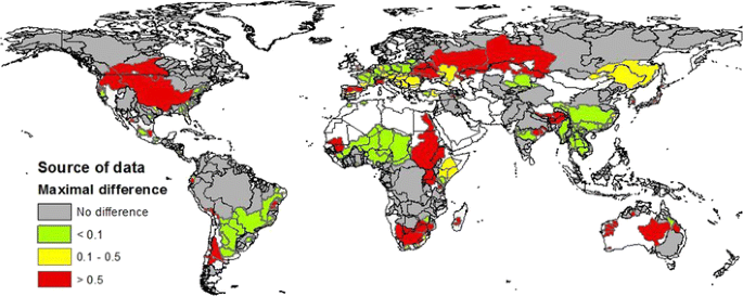
Absolute difference in scarcity indicators using model input data on water consumption and availability from WaterGap, Aquaduct or as used by the WFN. Results are obtained using M-BoulaySc, with values that range from 0 to 1
The three models providing the data are constructed differently. For the water availability data, WaterGap calculates water balances for each grid cell using climatic data and physiographic characteristics (soil type, slope, etc.), and these calculations are tested and calibrated to observed discharge data. Fekete et al. (2002) have used observed discharge data from monitoring stations to distribute runoff over a simulated river network, determined by a water balance model and the discharge observed. Aqueduct water availability is based on runoff data obtained from the Global Land Data Assimilation System version 2 (GLDAS2) (Rodell et al. 2004) and used to calculate the water available before and after human consumption. This is later assessed using withdrawal volumes, estimated from FAO AQUASTAT (Food and Agriculture Organization of the United Nations n.d.) reported withdrawal for each sector (domestic, industrial and agricultural) as functions of annually measured indicators such as GDP, population, irrigated area or electrical power production and combined with consumptive use ratios by sector by Shiklomanov and Rodda (2003). The WaterGap water use model is also based on these three sectors, and computes the water intensity (per unit use of water) for each sector and multiplies it by the driving force of water use: population, national electricity production and area of irrigated land and number of livestock for domestic, industrial and agricultural sectors, respectively. The WFN water consumption data are calculated using crop water use and production models from Mekonnen and Hoekstra (2011) and Fekete et al. (2002), and water withdrawals from Aquastat (a statistical database from FAO) are used along with consumptive use ratios of 5 and 10 % for industrial and domestic use, respectively.


Scarcity overview
The choice of model can have a significant impact on the scarcity results, since they differ in terms of consistency of response and absolute value. Among the most influential modeling choices, the scale at which the modeling data are used to calculate the index leads to important differences between sub-watershed and country scales. Maps shown in Fig. 7 identify regions in which collecting regionalised data at the sub-watershed level, rather than the country level, is relevant. While spatial resolution is an influential aspect, the question of the optimal scale remains. Variations in terms of water use and availability may be observed at a very small scale—perhaps a neighbor has a pond and not the other—but scarcity does not need to be defined at such a local level. Different scales may be relevant depending on the type of impact and region. Since scarcity is only associated with the modeling of impacts on human health (Kounina et al. 2013), the scale at which human society can still use water with no further adaptation to water scarcity is the most relevant and may range from a few kilometers that populations must walk in developing countries to larger areas that already get water from a mountain hundreds of kilometers away through pipelines, for example. Determining a scarcity index with no socio-economic context, although practical, may therefore have little relevance as a midpoint for assessment on human health. A region-specific optimal scale must still be determined, and inventory efforts must then be adapted to the scale, since variations are important even when using withdrawal-weighted averages. Temporal scale on the other hand showed a large variation throughout the year (large difference in many important regions between monthly and annual indicator), but these differences showed a high correlation between regions, meaning that absolute results would be affected but not so much comparative ones with same temporal inventory information.
In addition, the relationship that describes scarcity as a function of CTA (or WTA) was also shown to influence the results. The key issue is therefore how to define scarcity, and this is reflected in two choices: the choice of curve (direct, exponential or logistic) and the use of thresholds. On this later, both withdrawal-based methods and indexes (M-PfisterSc and M-SwissSc) use the OCDE thresholds at which a region faces moderate or severe water stress when respectively 20 or 40 % of the resource is withdrawn. While these thresholds are not defined based on scientific data, they at least provided a commonly agreed upon reference, which does not exist for consumption-based scarcity. This issue must be addressed in future research work, since scarcity is caused by water consumption and not simply withdrawal. Regarding the choice of curve, logistic and exponential curves correspond to opposite views in the assessment of regions with a high fraction of water use (a logistic curve results in smaller differences, whereas an exponential curve increases the difference). At this point, no robust data exist upon which to base this choice; hence, the direct curve represents the intermediate choice with the least added bias.
The source of the data is not important for most of the world when using M-BoulaySc, except for specific parts of the world (North America, Spain, Eastern Europe, East and South Africa, and other isolated watersheds) where differences are significant. The type of model and data reference year may be possible sources of discrepancy. The WaterGap water use data are for year 2000, and the water availability data are for 1961–1990. The WFN data average the 1996–2005 time period.
Finally, the differentiation between withdrawn surface water versus withdrawn ground water and the use of a WTA- or CTA-based indicator made less of a difference at a global level, with, however, a few important exceptions in specific regions. Moreover, it is uncertain whether surface and ground water scarcity are meaningful midpoints. While they lead to different potential human health impacts, greater ground water scarcity does not necessarily lead to more significant impacts, and perhaps, this distinction is only necessary when modeling endpoint damages, where impacts associated with a specific type of water can be assessed. Hence, this type of differentiation may be useful depending on the objective of the study and only for the regions highlighted in Fig. 6. Groundwater data of a satisfying quality are still not available and must be further developed from hydrological models.
3.2.3 Affected users
-
a.
Aquaculture
Though fisheries are important water users in certain parts of the world, the proportion of water used for this purpose in comparison to agriculture or domestic use is generally small (Boulay et al. 2011b). Consequently, including or excluding the impact pathway does not affect ranking and leads to an MDC of 0.0004, with the largest difference (absolute) seen for Egypt and China at 1.3 × 10⁻⁶ DALY/m3.
-
b.
Domestic
Comparing both hypotheses proposed in E-Boulay (marginal and distribution approaches) leads to an RCC of 83 % and an MDC of 0.75. The difference stems from attributing 100 % of the water deprivation to agriculture or using the fraction of water used by each user (i.e. including domestic users). The greater impacts of depriving domestic users result in a significant difference for all low- and middle-income countries with water scarcity (see map S8 in SI). This is because, even though domestic users represent a generally smaller fraction of users than agricultural (10–20 % of total use), the effect factors for domestic deprivation is higher than agricultural deprivation (Boulay et al. 2011b).
-
c.
Data source
The world average fraction of water used for agriculture across watersheds differs according to the data source: 46 % with WaterGap (used in E-Boulay), 61 % with Aquastat (used in E-Motoshita) and 65 % with Vorosmarty et al. (2000a) (used in E-Pfister). World-weighted averages using watersheds water withdrawal from WaterGap as a weighting factor yields 74 %, 72 % and 77 %, respectively. Calculating the same results with E-Boulay_agri in DALY from agricultural water deprivation with these three different data sources for distribution of affected users shows a change in RCC from 87 to 93 % and in MDC from 0.30 to 0.60. Aquastat and WaterGap are the best correlated with the smallest difference. Although the resulting difference is not as significant as the choice of model, for example, this discrepancy between models may be easily harmonised by selecting the data source believed as being the most robust. The difference may be observed in the relative difference between the SEE and CF of E-Pfister as compared with E-Motoshita_agri. Since only the distribution of affected users and scarcity differ between the SEE and CF and since they both use the same scarcity indicator, the difference in relative magnitude may be attributed to the user’s fraction of water use (see SI).
3.2.4 Socio-economic
The Motoshita_agri model differs significantly when considering (or not) the trade effect (RCC of 76 % and MDC of 1.32). When comparing Motoshita_noTE (instead of the original model) with E-Boulay_agri and E-Pfister, the correlation increases from 59 to 75 % (as compared with 53 to 49 % with the original model in Section 3.1.5), thus demonstrating the significance of the trade effect which is not present in the other models.
Overview of human health impacts
When modeling the human health impacts of water use, all three models agree that scarcity should be considered, followed by a parameter that describes the extent to which each user is affected (DAU) and an assessment of the socio-economic situation and, finally, an effect factor that quantifies the health impacts in DALY for each cubic meter for which a specific user is deprived. Differences arise out of the choice of scarcity indicator, but also out of the choice of users affected by water deprivation. Considering the effect on domestic users impacts the results and, although there is no consensus on whether they actually are affected or not, efforts towards a consensual model should consider this as a sensitive choice. Aquaculture/fisheries are only considered in E-Boulay and, although it is conceptually relevant to include it, it was shown to be insignificant for most of the world.
The trade effect factor introduced in E-Motoshita_agri had an important effect on the results, and, although still under development, the results indicate that further research into trade effects modeling is appropriate, since it constitutes an additional modeling step that is not yet included in other models. Excluding such effect could significantly change the conclusions of an assessment and underestimate water use impacts in richer countries. This is in agreement with the discussion in Boulay et al. (2011a) on the indirect impacts, and, ultimately, the two concepts should be combined: Agricultural water deprivation in a rich country either leads to an increase in imports and associated indirect impacts or to a reduction in exports with malnutrition-related human health consequences in developing importing countries. Whether this should be included in the characterisation factor or modeled separately as a model boundary extension should be agreed upon.
Although the effect factor from E-Motoshita_agri could not be directly compared, the value in DALY per cubic meter deprived for agriculture obtained by E-Pfister and E-Boulay were compared, and the value of Boulay is higher, as it assumes that malnutrition occurs proportionally to lack of irrigation water, whereas E-Pfister assumes that malnutrition occurs when all irrigation water necessary for food production has been consumed.
Lastly, it is important to keep in mind that, even though modeling choices are compared and general trends are uncovered, it does not certify that the damages that are modeled actually occur in the predicted way. Health damages are extremely hard to predict, and the relation between water consumption, scarcity and impacts is still at this point based on logical argumentation, and not a verified mechanism.
3.3 Uncertainty
The uncertainty associated with the choice of model is shown in Fig. 11 as the maximum difference between model results (max–min) for scarcity and human health deprivation for domestic and agricultural users. The numerical values of the confidence intervals for each model are provided in SI. While uncertainty may be high in certain regions, this is not the case everywhere (Fig. 11).

Uncertainty associated with the choice of model for a scarcity, b domestic water deprivation and c agricultural water deprivation
We only addressed the uncertainty associated to the choice of the model. The reader is invited to refer to other publications for more information about parameter and model uncertainty. Pfister and Hellweg (2011) addressed model uncertainty for the Pfister model; Bourgault et al. (2012) quantified the uncertainty of characterisation factors due to spatial variability within the Boulay method, and its parameter uncertainty is assessed in the upcoming impact model Impact World+ (Bulle et al. 2012).
The average values were shown along with the original models in Figs. S2, 3 and 4 (Electronic Supplementary Material), respectively, and the uncertainty data for each method are provided in SI. Although average values do not have any specific physical meaning, they are useful to carry out a sensitivity analysis on model choice. Uncertainty related to input data for WTA and socio-economic data has not been specifically addressed, since it was quantified for the case of M-Pfister and E-Pfister (Pfister and Hellweg 2011). However, the uncertainty may be combined for a complete uncertainty assessment.
4 Conclusions
Since several methods characterise the same impact pathways, it is not clear which method to use or the consequences of the choice of method. This paper provides such insight and sufficient practical geo-referenced information to guide the identification of regions in which different models and underlying modeling choices yield diverging results. Moreover, deconstructing the existing models and highlighting their differences and similarities has helped to determine building blocks to support the development of a consensual method. Until such a method is developed, the uncertainty related to model choice in each method as well as the average values at midpoint and endpoint can help enrich the results of one of the methods compared in this paper. In a related paper—under review at the moment of press (Water impact assessment methods analysis (Part B): Applicability for water footprinting and decision making, by the same authors) —the insights outlined in this paper were applied to a case study on laundry detergent. An assessment of the applicability of the different models and the related uncertainty was also carried out.
References
Aguilar-Manjarrez J (2006) WRI Major watersheds of the world delineation. FAO-Aquaculture Management and Conservation Service
Alcamo J, Henrichs T, Rosch T (2000) World water in 2025—global modeling and scenario analysis for the World Commission on Water for the 21st century. Kassel World Water series
Alcamo J, Doll P, Henrichs T, Kaspar F, Lehner B et al (2003a) Development and testing of the WaterGAP 2 global model of water use and availability. Hydrol Sci J 48(3):317–337
Alcamo J, Doll P, Henrichs T, Kaspar F, Lehner B et al (2003b) Global estimates of water withdrawals and availability under current and future “business-as-usual” conditions. Hydrol Sci J 48(3):339–348
Bauer C, Zapp P (2005) Towards generic factors for land Use and water consumption. In: Dubreuil A (ed) Life cycle assessment of metals: issues and research directions. SETAC - USA, Pensacola, USA
Bayart J-B et al (2010) Framework for assessment of off-stream freshwater use within LCA. Int J Life Cycle Assess 15(5):439
Bayart J-B et al (2014) The Water Impact Index: a simplified single-indicator approach for water footprinting. Int J Life Cycle Assess 19(6):1336–1344
Berger M, Finkbeiner M (2013) Methodological challenges in volumetric and impact-oriented water footprints. J Ind Ecol 17(1):79–89
Boulay A-M, Bouchard C et al (2011a) Categorizing water for LCA inventory. Int J Life Cycle Assess 16(7):639–651
Boulay A-M, Bulle C et al (2011b) Regional characterization of freshwater use in LCA: modeling direct impacts on human health. Environ Sci Technol 45(20):8948–8957
Bourgault G, Lesage P, Margni M, Bulle C, Boulay A-M, Samson, R (2012) Quantification of uncertainty of characterisation factors due to spatial variability. SETAC Europe 22nd Annual Meeting / 6th SETAC World Congress, Berlin.
Brent AC (2004) A life cycle impact assessment procedure with resource groups as areas of protection. Int J Life Cycle Assess 9(3):172–179
Bulle C, Humbert S, Jolliet O, Rosenbaum R, Margni M (2012) IMPACT World+: A new global regionalized life cycle impact assessment method, LCA XII, United States, Washington, Tacoma.
Fekete B, Vörösmarty C, Grabs W (2002) High-resolution fields of global runoff combining observed river discharge and simulated water balances. Global Biogeochem Cy 16(3):15.1-15-10
Fenner K et al (2005) Comparing estimates of persistence and long-range transport potential among multimedia models. Environ Sci Technol 39(7):1932–1942
Food and Agriculture Organization of the United Nations (nd.) AQUASTAT-FAO’s information system on water and agriculture. Available at: http://www.fao.org/NR/WATER/AQUASTAT/main/index.stm
Frischknecht R et al. (2008) Swiss ecological scarcity method: the new version 2006
Hertwich EG, McKone TE, Pease WS (1999) Parameter uncertainty and variability in evaluative fate and exposure models. Risk Anal 19(6):1193–1204
Hoekstra AY et al (2012) Global monthly water scarcity: blue water footprints versus blue water availability. PLoS ONE 7(2):e32688. doi:10.1371/journal.pone.0032688
Initiative, U.-S.L.C (2012) http://www.wulca-waterlca.org/
ISO 14046 (2014) Water footprint—principles, requirements and guidelines
Kounina A et al (2013) Review of methods addressing freshwater use in life cycle inventory and impact assessment. Int J Life Cycle Assess 18:707–721
Mekonnen MM, Hoekstra AY (2011) National water footprint accounts: the green, blue and grey water footprint of production and consumption. UNESCO-IHE, Delft, The Netherlands
Motoshita M, Itsubo N, Inaba A (2010a) Damage assessment of water scarcity for agricultural use 1. In: Proceedings of 9th international conference on EcoBalance. National Institute of Advanced Industrial Science and Technology (AIST), pp 3–6
Motoshita M, Itsubo N, Inaba A (2010b) Development of impact factors on damage to health by infectious diseases caused by domestic water scarcity. Int J Life Cycle Assess 16(1):65–73
Owens JW (2002) Water resources in life-cycle impact assessment: considerations in choosing category indicators. J Ind Ecol 5(2):37–54
Perry C (2007) Efficient irrigation; inefficient communication; flawed recommendations. Irrig Drain 56:367–378
Pfister S, Bayer P (2013) Monthly water stress: spatially and temporally explicit consumptive water footprint of global crop production. J Clean Prod. Available at: http://www.ifu.ethz.ch/ESD/downloads/reports/Monthly_WSI_LCA_FOOD.pdf
Pfister S, Koehler A, Hellweg S (2009) Assessing the environmental impacts of freshwater consumption in LCA. Environ Sci Technol 43(11):4098–4104
Pfister S, Hellweg S (2011) Surface water use – human health impacts. Report of the LC-IMPACT project (EC: FP7) (p. http://www.ifu.ethz.ch/ESD/downloads/Uncertainty_w). Retrieved from http://www.ifu.ethz.ch/ESD/downloads/Uncertainty_water_LCIA.pdf
Ridoutt BG, Pfister S (2010) A revised approach to water footprinting to make transparent the impacts of consumption and production on global freshwater scarcity. Glob Environ Chang 20(1):113–120
Ridoutt BG, Pfister S (2013) A new water footprint calculation method integrating consumptive and degradative water use into a single stand-alone weighted indicator. Int J Life Cycle Assess 18:204–207
Rodell M et al (2004) The global land data assimilation system. Bull Am Meteorol Soc 85(3):381–394
Rosenbaum R et al (2008) USEtox—the UNEP-SETAC toxicity model: recommended characterisation factors for human toxicity and freshwater ecotoxicity in life cycle impact assessment. Int J Life Cycle Assess 13(7):532–546
Shiklomanov IA, Rodda JC (2003) World water resources at the beginning of the 21st century. Cambridge University Press, Cambridge, UK
UNEP Global Environment Monitoring System (GEMS) Water programme (2009) GEMStat
Vorosmarty CJ et al (2000) Global water resources: vulnerability from climate change and population growth. Science 289(5477):284–288
Acknowledgements
The authors would like to acknowledge the contribution of Francis Gassert from the World Resource Institute (WRI) for providing data and understanding into the Aquaduct model. We acknowledge the financial support of the industrial partners in the International Chair in Life Cycle Assessment (a research unit of CIRAIG): ArcelorMittal, Bombardier, le Mouvement Desjardins, Hydro-Québec, LVMH, Michelin, Nestlé, RECYC-QUÉBEC, RONA, SAQ, Solvay, Total, Umicore, Veolia Environnement.
Author information
Authors and Affiliations
Corresponding author
Additional information
Responsible editor: Annette Koehler
Electronic supplementary material
Below is the link to the electronic supplementary material.
ESM 1
(DOCX 1530 kb)
Rights and permissions
About this article

Cite this article
Boulay, AM., Motoshita, M., Pfister, S. et al. Analysis of water use impact assessment methods (part A): evaluation of modeling choices based on a quantitative comparison of scarcity and human health indicators. Int J Life Cycle Assess 20, 139–160 (2015). https://doi.org/10.1007/s11367-014-0814-2
Received:
Accepted:
Published:
Issue Date:
DOI: https://doi.org/10.1007/s11367-014-0814-2