
Abstract
To setup efficient wireless mesh networks, it is fundamental to limit the overhead needed to localize a mobile user. A promising approach is to rely on a rendezvous-based location system where the current location of a mobile node is stored at specific nodes called locators. Nevertheless, such a solution has a drawback, which happens when the locator is far from the source–destination shortest path. This results in a triangular location problem and consequently in increased overhead of signaling messages. One solution to prevent this problem would be to place the locator as close as possible to the mobile node. This requires however to predict the mobile node’s location at all times. To obtain such information, we define a mobility prediction model (an agenda) that, for each node, specifies the mesh router that is likely to be the closest to the mobile node at specific time periods. The location service that we propose formalizes the integration of the agenda with the management of location servers in a coherent and self-organized fashion. To evaluate the performance of our system compared to traditional approaches, we use two real-life mobility datasets of Wi-Fi devices in the Dartmouth campus and Taxicabs in the bay area of San Francisco. We show that our strategy significantly outperforms traditional solutions; we obtain gains ranging from 39 to 72% compared to the centralized scheme and more than 35% compared to a traditional rendezvous-based solution.
1 Introduction
Wireless mesh networks (WMNs) offer the potential to deploy ubiquitous wireless access at low cost for mobile clients through a flexible wireless multi-hop backbone [1, 2]. Nevertheless, recent experimentations have shown that multi-hop wireless infrastructures suffer from several technical limitations that prevent its rapid adoption. For instance, the wireless medium access protocol introduces fluctuating transmission delays and the network performance dramatically decreases with traffic load [3, 4]. On top of that, node mobility, which has become an inherent characteristic of wireless networks, introduces extra-overhead in location management and forwarding services to assure communication reliability. In order to envision wider deployments of WMNs, new network services have to be specifically designed to fit mobility constraints.
An efficient location service is fundamental to any network that involves node mobility. By efficiency, we mean that the system must be able to: (1) provide accurate location information at anytime and (2) achieve its goals at low control overhead. This latter point is particularly important because of the scarce resources of wireless networks. In this paper, we focus on a WMN spanning a metropolitan area containing a large number of routers providing connectivity to a large number of regular mobile nodes. We address the problem of reducing the overhead used to maintain up-to-date location information at location servers (or locators).
In general, location services in wireless mesh networks must be self-organizing, as nodes cannot rely on a prior infrastructure. Besides the standard centralized approach, an interesting way to provide scalable and distributed location service is to rely on the concept of distributed hash table (DHT) [5–7]. In such schemes, location updates generated by mobile nodes (MNs) and location lookups generated by corresponding nodes (CNs) must be forwarded to a locator, which is determined according to an hash function on the MN’s identifier. However, the location of this locator can be potentially far from the nodes’ positions—is is known as the triangular location problem.
In our approach, we tackle the functionality of locator as a mobile service. According to the mobility behavior of the MN from a per-node view, we propose to place the location functionality (and, consequently, the locators) at wireless mesh routers (WMRs) that are likely to be close to (if not at) the current position of the node. The goal is to limit the effects of triangular location. Note that such an approach requires the system to know the current location of each MN, which seems contradictory because this is exactly the goal of the location service. A possibility to solve this chicken-and-egg problem is to rely on prediction of the node’s mobility behavior to define the most appropriate WMR that will play the role of locator. It has been shown in the literature that users follow daily routines and that mobility patterns have cyclic properties [8–11]. We rely on such principles to propose a location service that benefits from the periodic nature of mobility to push locators close to mobile nodes.
Our proposal is structured in two parts: an agenda-based prediction model and an agenda-based location service. These components are complementary and run on top of a traditional DHT-based location service. As explained in the following, the idea is to benefit from periodicity whenever possible.
The first contribution is the definition of an agenda-based prediction model. Existing approaches are either based on next association prediction from the node current state [12] or rely on a typical mobility pattern from combined mobility history [13]. Our prediction model, instead, provides locations independently from the current state and reproduces the multi-scale periodicity aspect of mobility behaviors in the form of an agenda. A node may visit one particular place every Monday and another place twice on Tuesdays. Furthermore, locations are associated with well-determined time slots in a day (which explains the “agenda-based” terminology). Hence, we establish a direct correspondence between the visited location at time slot t and the visited location at t + period, where period is, in our case, 1 week. A typical entry in the agenda is “Next Monday, from 7 am to 9 am, node x will likely be located around mesh router 256.”
The second contribution is the design of an agenda-based location service. It is composed of two levels of indirection. The basic level uses a DHT to determine the anchor router of a mobile node. Contrary to existing solutions, the anchor does not store the current location of the mobile node, but its agenda. Correspondent nodes first fetch the agenda and use the enclosed information to determine the locators of the node, which are the mesh routers the MN is expected to get associated with. In the example of the previous paragraph, the locator for the node during the period “Monday, 7 am–9 am” is mesh router 256.
To validate our scheme, we analyze our proposal using publicly available traces. In two companion papers [14, 15], we analyzed predictions robustness and discussed some preliminary results using the Dartmouth campus dataset [16], which show that over an observation period of 59 weeks, mobile nodes spend 80% of their time at a maximum distance of one hop from their expected location server. Furthermore, 81% of the location update messages are constrained within this one-hop radius. This drastically reduces the propagation areas and then the number of operated transmissions when compared for instance with centralized and DHT-based approaches. In this paper, we make a step forward by integrating the agenda-based location service and by performing a deeper analysis using the Dartmouth campus dataset and another trace representing the mobility of taxi cabs. Our system leads to gains in terms of reduction of signaling overhead ranging from 39 to 72% compared to the centralized scheme and more than 35% compared to a traditional rendezvous-based solution.
The remainder of this paper is organized as follows. In Sect. 2, we detail the principles of traditional location management approaches and investigate the different means to reduce control overhead. In Sect. 3, we introduce the basic idea that drives our approach as well as its operating principles. We further detail our location management system through the creation of the agendas and their integration into the global architecture. We present the preliminary results obtained using the Dartmouth dataset in Sect. 4. The performance of our proposal is compared with other traditional approaches using both Dartmouth and Taxicabs datasets in Sect. 5. In Sect. 6, we discuss the related work and conclude this paper in Sect. 7.
2 Reducing location management overhead
In this paper, we consider infrastructure-based location services, which involve three types of messages that are potential sources of overhead. Update messages are sent by a MN to its locator to inform its current location. Lookup messages are sent by the CNs willing to communicate with the MN, and reply messages sent by the locator to the CNs as a response to the lookups. Note that each lookup message generates a counterpart reply (these messages are depicted in Fig. 1).

Messages involved in the location service
Compared to a cellular network, there are no hierarchy between wireless routers, i.e., all routers serve the backbone and provide connectivity to MNs. A router can play the role of locator for one or several nodes at any time and for varying durations. Furthermore, we assume that each association generates an update. In this context, we consider the efficiency of a location service as based on the number of transmissions operated between wireless routers to ensure the service operation.
2.1 Existing infrastructure-based location approaches
We can cite at least four traditional (non exclusive) infrastructure-based strategies to perform location management: centralized, DHT-based, local-anchor, and hierarchical approaches. Although not specifically designed for wireless mesh networks, these approaches will serve as basis for our comparisons later in this paper.
2.1.1 Centralized architecture
The centralized scheme is a widely used strategy. Wired-based infrastructure networks use centralized and two-tier strategies (HLR in GSM [17] and Mobile IP [18] in the Internet) because of their simplicity of maintenance. At each association, a node sends a position update to the central locator. Lookups are also sent to the central point. Note that this approach may suffer from successive long update paths when mobile nodes are far from the locator.
2.1.2 DHT-based schemes
A DHT-based system relies on a set of servers (locators) and a hash function. The locators participating in the system share the set of values in the image of the hash function. This function is applied on the permanent identifier of a node and the resulting value indicates the locator that stores the node’s location information. Each time a node changes of access point it must update its location information at its corresponding locator. To retrieve some node’s current location information, the CN applies the hash function on the identifier of the node, which gives the same locator. For further details on the functioning of DHT-based location services, the reader is invited to refer to the many papers in the literature [19–21].
2.1.3 Local-anchor strategies
In the local anchor strategy, local servers (specifically called “anchors”) filter successive updates sent from the same administered region to a central locator [22]. When a node moves within a region, only one synchronization message is generated (when the node enters the region) from the local server to the locator. Such an approach drastically reduces the number of updates sent beyond the concerned region but does not contribute to reduce the load from the lookup standpoint. Furthermore, updates and synchronization messages may be generated up to the central locator if the node re-associates after a disconnection.
2.1.4 Hierarchical strategies
In hierarchical systems [6, 7, 23, 24], locators are organized in a tree where each leaf manages location information of all nodes inside a region of the network. When a new node appears, its location information is recorded along the branch, from the closest leaf to the root (the default locator). Any update only affects the sub-tree under the least common ancestor (LCA) along the old branch and the new one. In this context, we call synchronization messages the updates that are sent from the managing locator to the LCA. Consequently, if a node moves in a contiguous region, the transmission of signaling messages is limited to a few links. In the same manner, location lookups are transmitted until an intermediate server that has the information is found. However, if one user has cross-regions mobility, high macro-mobility, and/or has to often disconnect from the network, updates may get frequent access to higher level of the tree. Therefore, mobility of nodes may lead to an erratic signaling behavior. Also, as in the previous case, re-associations lead to unnecessary updates and synchronization messages sent up to the central locator.
2.2 Where to improve?
We address the problem of reducing the overhead generated for location management as a problem of locator placement. In the following, we investigate the general conditions for optimizing such an operation.
Let us consider a network composed by a set of N nodes evenly positioned in the network. Let \(U_{m\rightarrow loc}\) be the total cost, in terms of number of hops (transmissions), of the distribution of number of updates sent at different distances from the MN m to the locator. Synchronization messages used in some location services are considered as included in U. Assuming that the cost of sending a lookup is the same than the cost of receiving a reply , \(L_{i\leftrightarrow loc}\) is the total cost in terms of number of lookups triggered and replies exchanged between CN i and the locator. The total signaling cost C m generated in the network can then be written as:
The total cost can be reduced by tuning either of the terms of the right-hand side of the equation. Reducing the sum ∑L is difficult to achieve because the system does not know a priori where the correspondent nodes are. Hence, an alternative solution would be for the system to minimize U. There are two ways to achieve this goal, either by forcing the MN to stay directly associated with its locator, which is obviously not realistic as it prevents mobility, or by pushing the locator close to the current location of the MN. This second alternative is exactly what our proposal is about.
3 Agenda-based location service
In this section, we explain how an agenda can be used as the main support of a location service.
3.1 Overview
Two levels of services compose our location management system:
-
1.
Global service. This service determines the anchor of a node, in a similar way to traditional DHT-based solutions. The difference here is that the anchor does not store the current location of a node; instead, it returns the agenda of the node in question (see in the following subsection how an agenda is created). As we will see in the following, the agenda is available for a reasonable amount of time and thus can be cached by the corresponding node to prevent frequent access to the global service.
-
2.
Local service. Locators are points in the infrastructure that effectively know at a given time where mobile nodes are. They respond to lookup requests and inform about the current position of mobile nodes. To determine which of its locators is currently in charge of storing its location, a mobile node refers to its agenda. As a locator is chosen by a mobile node because of its high probability of being close to it, location updates remain localized. We explain in details how the location service operates in Sect. 3.3.
3.2 Creating the agendas
The considered mobility model assumes the mobility of the nodes as a combination of two components: (1) mobility inside areas of interest and (2) mobility between areas of interest. An area of interest is basically a region in the network where a node remains a certain amount of time. It can be for example a hotspot, a building, or a house. While mobility between areas of interest is operated with the desire of moving to a different destination, mobility within areas of interest could be characterized by the desire of visiting one or several sub-locations (e.g., different offices or floors of a building). Furthermore, mobility within an area of interest can be considered harmful as short movements and ping-pong effects imply the generation of a large number of location updates.
To limit the propagation of location updates, our approach (1) investigates the areas of interest of a node and when they are likely to be visited and (2) determines the correct position in order to place a locator. The purpose of an agenda of locators is to reflect the succession of visited areas of interest by providing the location (recall, the WMR a node is associated with) at different time slots. We explain in the following how to create and manage agendas of locators. A more detailed analysis is available in [14].
To reduce the frequency of access to the global service and temporal stability of locator assignment, an agenda of locators provides long-term predictions and is based on a format that is not synchronized with the observed mobility patterns. The operation of the algorithm considers the global prediction period as a succession of time intervals where, in each of them, the visited area of interest is determined as the center of gravity of a cluster of WMRs. Without loss of generality, the global prediction period covers a window of 7 days, from the Monday through Sunday, where each day is sliced in N time periods of equal duration D. We consider N = 24 and D = 1 h. We will see later in Sect. 4 that these values are pretty well adapted to the context of human mobility. In the rest of this paper, we will refer to this period of 7 days as a cycle of predictions. One might consider that, with this specific slicing strategy, the list of (day, hour) pairs a node provides can be represented as an “agenda” (see Fig. 2 for an illustration of this structure).

Example of representation of an agenda of locators. Empty slots represent periods during which the node does not present any clear association pattern
For a particular time period, the choice of the most appropriate WMR to play the role of locator is made according to temporal and spatial aspects of the mobility of the node. By observing its past and current mobility behavior, during a time period, the predominant “place” (in terms of duration of association) and prevalent (through past mobility history) is selected. A place can be one or a group of nearby WMRs. If there is only one WMR, the place is identified by the ID of the WMR. When more than one WMR are candidates, we gather them into a single cluster and use the most predominant WMR as the ID of the location. We use a clustering algorithm based on the roaming events as distance metric and so do not use any geographic information (a complete description of the clustering scheme is available in [25]). It is also possible, however, to use other algorithms based on geographical information [26, 27].
The management of mobility history is designed to be reactive to changes in the node’s mobility behavior. The mobility history is obtained by gathering the latest k agendas (k = 0 corresponds to the current observed week). To define the retained areas of interest for a particular time period, we consider two cases: (1) the duration of associations within an area is equal to D and (2) the duration of association is shorter than D. If the duration is equal to D, we suppose that the observed mobility behavior within the time period will have a high probability to occur again in the same time period of the following week. Thus, this area is retained for the final prediction. If the duration is shorter than D, the area that has been prevalent through the weeks is retained for that time period. Among these areas is considered the area that has had more occurrences in the mobility history for the considered time period.
An agenda is also associated with an agenda counter to track the updates and a period of validity. In this paper, we consider that the period of validity is 1 week for all the agendas and then, every week a new agenda is generated.
The creation of the agenda is based on the observation of the mobility patterns of the node. This approach raises two important issues: (1) because of the lack of node’s activity, the agenda might present some empty slots (as shown in Fig. 2) and (2) the mobility of the node has to be monitored for at least 1 week to generate the first agenda (bootstrap issue). Considering the global service as a backup system can solve both issues; when there is no information about some time period, the anchor node (obtained through the DHT-based service) plays the role of locator. However, to minimize the access to the global service, we chose to fill up empty slots with the locator indicated in the previous slot. Hence, we do not consider the existence of a backup system in this paper.
Now that all entities forming our location service have been described and how agenda of locators are created and managed, we explain in the next section how the service operates according to the mobility of the locators.
3.3 Service operation: location updates
Whenever a node is present in the network, its current position has to be registered at its active locator and a valid agenda must be available through the global mapping service. These are the requirements for the coherence of the location system. At each time period, the active locator may change and the agenda has to be renewed at each cycle of predictions. In this way, each node must provide the network with the necessary information to maintain this coherent state at specific steps:
-
At the beginning of each cycle. Agendas of locators are valid until the end of the current cycle of predictions. At the beginning of each cycle, the node has to generate a new agenda taking into account its recent and past mobility information. Once updated, it sends the new agenda to the global mapping server where it can always be fetched by CNs (arrow 0 in Fig. 3).
Fig. 3 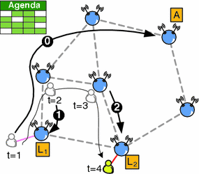
The location service operation. “A” stands for anchor and [“L1”,“L2”] stand for locators 1 and 2, respectively. From time to time (every cycle of predictions), the MN updates its agenda of locators in the global mapping system (arrow 0). At each association and time period, the MN registers its current position at its active locator, which changes according to the node’s predicted mobility pattern (arrow 1 during period 1, arrow 2 during period 2)
-
At the beginning of each time period and at each association. The MN sends a location update to the locator in charge (arrows 1 and 2 in Fig. 3). In this message, the node provides the network address of the WMR it is associated with, as well as the corresponding validity period. While location updates generated at each association have a mobility tracking purpose, by doing this at the beginning of each time period, MNs indicate that they are still present in the network, as a heartbeat system does. This is also useful for nodes that remain static during several consecutive time periods.

It is important to underline here that, if prediction is correct, most of the time updates are not sent, as the destination of the updates would be the WMR the mobile node is associated with.
3.4 Service operation: lookups
Nodes follow the succession of locators provided in their agendas to update their current position. To be able to retrieve such information, a CN must first fetch a copy of the agenda of the destination node from the global mapping system. Two situations may occur:
-
The destination node’s agenda is unknown. To obtain the agenda of a MN, the CN sends an agenda-request message to the WMR it is associated with, providing the identifier of the destination node. The WMR applies a hash function on the identifier of the destination node to identify the mapping server in charge (i.e., the anchor). Once determined, it forwards this agenda request to the anchor. This latter returns a copy of the agenda to the node if the agenda is valid for the current cycle of predictions. If it is not valid, this means the destination node is not yet associated in the network. In this case, the server returns an agenda-miss message.
-
The CN already has a valid copy of the MN’s agenda. The CN is then able to determine the current active locator for the destination node. To obtain the current position of the node, it sends a location request to this locator (indicated in the agenda). The locator responds with a location-response providing the current position of the destination node. It replies with an unreachable-node message if the MN has not updated its current position.
We have described the complete architecture of our location service, the entities, interactions, and operations. In the following, we discuss the parameters that would have an impact on the performance of our system.
3.5 Cost of the agenda-based system
Our global location service introduces a new signaling cost, as we need to store and fetch agendas before being able to use the enclosed information. However, the idea behind this system is that the access to the global service is not function of nodes mobility behavior.
With our local location service, we wish to reduce the distances between the MNs and their assigned locators to minimize the amount of transmissions of update messages. Let \(U_{m\rightarrow loc}\) be the total cost of updates sent at different distances between MN m and its assigned locator and \(L_{i\leftrightarrow loc}\) be the total cost of lookups/replies exchanged at different distances between CN i and the assigned locator of MN m . Eq. 1 can be rewritten as:
where \(U_{m\rightarrow anch}\) is the cost for node MN m to send its agenda to its anchor and \(L_{i\leftrightarrow anch}\) is the cost for node CN i to retrieve this agenda (which include one query and one reply).
Through the local service, our purpose is to obtain \((U_{m\rightarrow loc} + U_{m\rightarrow anch})\) as low as possible. To achieve this goal, the predictions provided in the agendas are designed to position locators as close as possible from the MN. An agenda remains valid for a certain period, after which it must be renewed at the corresponding anchor (synchronization messages). Hence, the cost \(U_{m\rightarrow anch}\) is directly dependent of the frequency of generation of agendas. In this paper, we consider that the agendas are generated once a week. If MNs are highly mobile, the treatment of the agendas will tend to be negligible. Nevertheless, our service, for the updates management part, will be not efficient if MNs are static. In this situation, the cost of transmitting agendas to anchors becomes greater than treating the updates. In the same way, if CNs initiate communications with MNs only once a prediction period (1 week), the cost of fetching agendas will be as important as treating lookup messages. In the opposite case, the cost of fetching agendas becomes negligible.
Assuming that nodes are mainly mobile and that CNs initiate communications with MNs regularly, the main parameter that will affect the performance of our system is nodes mobility behavior. Hence, we focus our performance analysis to the study of the impact of real mobility behaviors on our prediction algorithm and on the overall operation of our system.
4 Evaluation of the agenda accuracy
In this section, we evaluate our system according to the Dartmouth dataset under two perspectives. First, we validate our assumptions that agendas do provide an accurate means to represent node mobility. We evaluate then the locator placement and the cost of the update messages in terms of number of hops.
We compare our approach with a flat DHT-based location service. We assign to each node one global mapping server according to a MD5 operation on its identifier. We vary the number of servers participating in the DHT; we refer to each configuration as a n-DHT system (with n varying from 1 to 512 servers randomly placed throughout the network). We run each setup 100 times.
Finally, we evaluate the accuracy of locator prediction through both the duration of association that nodes have spent at different distances from the locator position and the path lengths of all location updates.
4.1 Setup
To evaluate the performances of our location service, we need real mobility data traces from an environment where we will be able to observe nodes mobility according to a fixed infrastructure. Due to the lack of data traces focused on nodes mobility behaviors in real WMNs, we chose to extrapolate a WMN topology from a conventional IEEE 802.11 wireless network. The dataset we use represents 3 years (2001-04-11 to 2004-06-30) of collected information about all wireless adapters connected to the wireless access network of Dartmouth campus. The campus is composed of 188 buildings covered by 566 official access-points (APs) on 200 acres and about 5,500 students. From this dataset, we chose a subset of 4,961 mobile nodes over an observation period of 59 weeks (between the first Monday of January 2003 to the last Sunday of February 2004).
We measure path lengths between position of the MNs and their predicted locators. The infrastructure of the wireless network of the Dartmouth campus is composed by APs (that will represent our WMRs). To evaluate our system in a wireless mesh network context, we virtually interconnect the overall topology by wireless links between the APs. The algorithm that we used to obtain a wireless mesh topology from the known topology of the campus network and from the roaming events of the MNs is based on three steps:
-
Interconnect APs with coordinates. We have the coordinates of 506 APs out of the 590 visited. The first step of the algorithm is then to interconnect these 506 APs on the basis of average radio coverage.
-
Interconnect APs involved in short-term handoffs. The second step is to attach to the obtained topology the APs that do not have coordinates but that have been involved in roaming events where the duration of handoffs was less or equal to 1 s. In this step, 45 APs have been included in the topology.
-
Interconnect the remainder APs. In this step, we only link the remainder APs that have been involved in roaming events with the already obtained topology. The interconnection is made on the basis of the smallest duration of handoff and we consider this link as obtained with the use of directional antennas.
With this algorithm, we obtained a wireless mesh topology, which has a diameter of 19 hops.
4.2 Positioning locators
We show in the following that predictions shown in agendas lead to shorter paths for location updates. We evaluate how long nodes stay at different distances from the active locator. We specifically analyze the duration of the time nodes spend at different distances from the active locator as well as from their anchor nodes (the one obtained by a DHT in the global service). Figure 4 shows that nodes remain, in average, 57% of their time directly associated with their predicted locators and 23% of their time at only one hop away from them. Cumulated, nodes remained 80% of their time at a maximum of one hop away from their expected positions. Concerning n-DHT systems, whatever the number of servers of the system, the nodes were, in average, 76% of their time between 3 and 7 hops from their assigned mapping server which is high for a 19-hops network diameter. One of the reasons for such a good result is that nodes have prevalent places in the network such as home locations (places where a node spends more than 50% of its time).

Percentage of time nodes had spent associated according to the distance to the active locators (4,961 nodes). We can observe that n-DHT results are overlapped
4.3 Cost of updates
Recall that correctly positioning locators does not necessarily indicate that we succeed to reduce the cost of update messages. Indeed, nodes might for instance be static at specific places for long periods and have high micro-mobility and/or undergo ping-pong effects in other places. The first purpose of the following analysis is to evaluate if unnecessary location updates are well handled by our approach, i.e., if the path followed by location updates, if any, remains short. Secondly, to evaluate the total cost of update messages and then the gain compared to n-DHT systems.
Figure 5 evaluates the average number of location updates that have been generated and forwarded at different distances from the active locator. This figure is similar to Fig. 4 but indicates the number of messages generated instead of the time spent at some place. As in the previous analysis, most of the location updates (≈81%) have been generated between 0 and 1 hop. Clearly, the path length of location updates are not upper bounded. Note however that we succeed to limit the path length of more than 85% of the messages to a radius of 2 hops from the assigned locator. With n-DHT approaches most of the location updates have been generated between 3 and 7 hops, which is far from being negligible in a 19-hop network diameter.

Average number of location updates generated at different distances (hops) from the assigned locator/anchor
In n-DHT approaches, nodes are not constrained by the time slicing. In our approach, at the beginning of each time period, the nodes have to send location updates as a heartbeat system, which explains why the number of location updates generated is greater. Furthermore, at the beginning of each cycle of prediction, nodes have to update their agendas in their assigned anchors, which constitutes the second part of the overhead.
This figure also comforts the fact that, with our system, problematic location updates are well handled. Indeed, as nodes spend most of the time associated to their active locator, the high number of generated location updates at 0 and 1 hop indicates that they have had high micro-mobility between the active locator and the neighboring WMRs.
To evaluate the total cost of location updates in terms of number of transmissions operated between routers, the Fig. 6 presents the CDF of the percentage of transmissions operated according to the distance between the locator/anchor and the MN. The percentages of each system are computed according to the system that has operated the greatest number of transmissions—here, the 512-DHT system with an average number of 66,357,336 transmissions. As in Fig. 5, n-DHT systems’ plots roughly superpose with each other showing the same total number of transmissions operated (there is a difference of 2.33% between the centralized scheme and the 512-DHT scheme). There is a wide gap between the total number of transmissions operated between our approach and n-DHT systems. With a number of transmissions of 21,695,504 44,661,833, our approach leads to a gain of 67%.

CDF of the average number of transmissions operated according to the distances between the locator/anchor and the MNs. The percentages of each system are computed according to the system that has operated the greatest number of transmissions (here the 512-DHT system)
As a summary, in this particular topology and with the nodes that we observed, we succeed to position locators most of the time directly in places where mobile nodes are likely to spend their time. With our approach, most of the location updates generated have been contained to up to one hop from the positions of the active locators.
5 Evaluation of the global location service
In this section, we compare the performance of our approach with traditional location services using two mobility traces. We explicitly make the distinction between the cost of updates generated by the nodes towards the locators and the cost of synchronization messages generated by the location service to handle the location information. We evaluate our system according to the Dartmouth dataset and another real mobility scenario that represent movement of taxis in the bay area of San Francisco, California, USA. The latter, referred as “Taxicabs dataset” is composed by 542 nodes that have been GPS tracked during an observation period of 1 month.
In the preceding section, we have evaluated our proposal according to a mesh topology close to the network configuration of the Dartmouth campus. In this section, we compare our approach with hierarchical, local anchor, DHT, and centralized schemes. These schemes have been designed for cellular-like networks. Such type of networks is organized in non-overlapping cells aggregated into contiguous geographical regions called Registration Areas (RA). In the taxicabs dataset, there is no natural notion of WMN-type topology. We propose to generate new generic mesh topologies for both Dartmouth and Taxicabs datasets. Footnote 1 We choose a grid topology to avoid the presence of dense topological areas. Mesh routers are uniformly positioned in the grid cells. To retrieve nodes mobility patterns according to the generated topologies, we rely on the geographic trajectories available in the Taxicabs dataset and that we have estimated for the Dartmouth dataset.
We further describe below each approach that will be used as a base for comparison with our agenda-based solution.
6 Topology
In a wireless mesh network two neighboring routers have to be within radio range of each other. Rather than defining a realistic radio range, we fix this range according to the environment size in order to control the number of mesh routers to create. We keep this number low to be able to run graph algorithms in a reasonable amount of time.
The algorithm to generate the topology is simple and is the same for both datasets. It first defines the environment area according to the minimum (x, y) position and the maximum one observed in the movement traces. In the taxicabs dataset, we voluntarily discard movements that happened more than 40 km away from San Francisco’s downtown (which is our origin in the geographical plane) so that we do not explode the number of mesh routers to generate a grid topology for the taxicabs dataset. We then define a radio range radius r and position a mesh router every r meters in a grid fashion. For the Dartmouth dataset, by setting r = 100 m, the result is an environment of 2, 688 × 1, 877 m for a total of 513 mesh routers. For the taxicabs dataset, by setting r = 1,000 m, the result is an environment of 71, 435 × 63, 353 m for a total of 4,608 mesh routers. Note that in both datasets, the middle points of the topologies correspond to highly popular places (the San Francisco’s financial center for the taxicabs dataset and near the Baker library in the Dartmouth dataset).
For both datasets, each movement trace has been rewritten so that geographical coordinates point now on the identifier of the closest mesh router.
6.1 Approaches in comparison
We now detail how the different approaches will be compared. We arbitrary define for all approaches that consider regions of management, which are regions of up to 2 hops. Approaches that introduce a random part are run 100 times to obtain an average value. We compare the performance of our agenda-based location system with the centralized approach, a DHT-based system, the local anchor strategy, and the hierarchical one.
In the centralized strategy (noted “Cent”), a mesh router is randomly chosen as the final location database for all mobile nodes. In the DHT-based system, we define a set of 32 location servers and assign randomly to each mobile node one of these servers as the node’s locator. One location update generated is first forwarded to the closest DHT server and finally forwarded to the assigned locator. These two location strategies serve mainly as a basis of comparison. They also help evaluating the performance of a randomized management solution.
In the hierarchical solution (noted “Hier”), the considered tree organization may have an impact on the performance of the system (one managed area can cover only a part of a highly popular place generating a ping-pong effect). Therefore, we propose two different algorithms to generate the tree: the first (noted “Fix”) is based on a hierarchical segmentation where the root of the tree is positioned in the middle of the grid and the last leaves on the borders (see Fig. 7a). The second is more a distributed “self-organized” algorithm (noted “Dis”) where the root is positioned randomly. From the root position, the second level of the tree is selected by taking all possible mesh routers at the border of the root’s managed area so that each selected router manage an independent area of 0–2 hops. The algorithm continues to generate regions as long as there are non-managed mesh routers at least 3-hops away from the closest region manager (see Fig. 7b).

a Model of pre-determined regions partition: the root is in the middle of the environment. b Model of regions partition with the self-organized algorithm: the root position is chosen randomly
For the local anchor strategy (noted “LA”), we rely on a static approach where, when the mobile node enters a managed region, it is assigned to the anchor that manages this RA. We use the same resulting regions segmentation obtained for the hierarchical solution but without the hierarchical organization. However, the final database is positioned randomly.
6.2 Results
For the performance evaluation, we keep the distinction between the costs of signaling messages generated for position updates and for synchronization. We consider that all messages (updates, agendas, synchronization) have the same size. In our agenda-based approach, we consider synchronization messages as the transmission of agendas from mobile nodes to the assigned DHT servers. According to the strategy, an update message does not always generate a synchronization message across the distributed entities of the location architecture (the filtering in the local anchor strategy for instance). Therefore, we analyze separately the number of generated messages for both operations (update, synchronization) and present each percentage (the sum of percentages of updates and synchronization makes 100%). Recall that we do not include de-registration messages and signaling messages to construct and maintain the architecture coherent, although this could drastically increase the signaling overhead (the DHT system for instance). Figure 8a shows the CDF of the percentage of position updates generated (Fig. 8c for the synchronization messages) according to the number of transmissions that have been operated for their forwarding in the Dartmouth dataset. Similarly, Fig. 8b and d show the results for the taxicabs dataset. The performance of the centralized strategy appears only in Fig. 8a, b, as there are no synchronization messages introduced.

Performance of location strategies in the Dartmouth and Taxicabs dataset. a and b CDFs of the percentage of position updates according to the number of operated transmissions. c and d CDFs of the percentage of synchronization messages according to the number of operated transmissions. e and f Gain in percentage of the total number of operated transmissions compared to the centralized approach
The CDFs show similar patterns for update messages in both datasets. The closest region manager can be joined in up to 2 hops in the hierarchical and local anchor strategies, for both types of hierarchy and region partitioning (Dis and Fix). Because there is a signaling message generated for each received update in the hierarchical strategy, the percentage is bounded to 50%. One can observe that, compared to the centralized strategy, the DHT and our agenda-based strategies have points in common. The locators in our agenda-based solution act like final databases during a predefined period. Therefore, the CDFs are comparable, but the objective is to have a median path length as close as possible to 0. In the Dartmouth dataset, we succeed to limit more than 76% of messages to 2 hops for a gain of almost 15 hops at some points compared to the centralized strategy. However, the efficiency of predictions is not the same in the taxicabs dataset. Although 90% of messages have been contained in less than 20 hops, more than 50% show path lengths greater than 4 hops. Nonetheless, compared to the centralized strategy, we still have an important gain of more than 20 hops for most of the messages.
There are far less similarities in the CDFs of synchronization messages. Compared to the performance of the DHT strategy, one can observe that messages generated with the hierarchical strategy have required fewer transmissions in the taxicabs dataset than in the Dartmouth dataset (shift to the left). The main reason for this is that there are no disconnections in the taxicabs mobility. This phenomenon has a high impact in the hierarchical strategy as there is only one signaling message addressed to the root database for each mobile node. In the local anchor strategy, one can observe that most of messages require much more transmissions than for the DHT strategy. Although less than 30% of messages are generated with the fixed organization, they are mostly transmitted between 50 and 80 links, which increases considerably the total cost.
On the other hand, the DHT strategy and our agenda-based solution present highly similar patterns. If the CDF for the DHT strategy can be explained simply as the result of a typical centralized scheme (and then a Gaussian pattern in the probability density function), the curve obtained with our agenda-based strategy is the result of a control of the number of times agendas are sent each prediction period. The number of generated messages with our solution is basically the result of the number of observed weeks multiplied by the number of nodes active each week. Although we do not limit the path lengths, being able to control their number is an important asset.
We now quantify the costs of all strategies. Because the number of operated transmissions is different in all approaches, we use the centralized approach as a basis and quantify the difference in percentage of operated transmissions for the other approaches in Fig. 8e for the Dartmouth dataset and in Fig. 8f for the taxicabs dataset. Surprisingly, the centralized strategy is not the worst approach in both datasets. It has comparable or even better performance than the local anchor and hierarchical strategies. One can understand that the DHT scheme has in average the same shift in performance (around −10%) because of a possible indirection. In the Dartmouth dataset, because of the recorded disconnections, the local anchor strategy suffers from the region partitioning as it imposes an indirection to the region manager. In the taxicabs dataset, the high mobility generates the same behavior where the local anchor strategy needs to continuously communicate with the root database. However, we now see clearly that regions partitioning has a strong impact on the performance. With fixed partitions, all regions have almost the same size which somewhat helps to reduce successive handoff between regions.
Globally, the hierarchical strategy finds a real gain when mobile nodes do not disconnect, as using LCA (least common ancestor) allows reducing path lengths. One can however note that the performance of the hierarchical strategy depends on several parameters over which the network may not have control: (1) the regions partitioning that, in a self-organized network, may not be as efficient as the fixed segmentation and (2) disconnections. In an IEEE 802.11 wireless mesh network, we may assume that, because of energy consumption, nodes may need to disconnect regularly. According to these parameters, we can observe that our agenda-based system provides important gain in both datasets (compared to the best hierarchical results), while being compatible with a self-organized network. The agenda-based strategy is only dependent on the number of active nodes and on the periodicity of mobility patterns.
7 Related work
Location management has been a prolific research area in recent literature on wireless networking. The works that are the closest to ours have been specifically developed in the context of cellular networks and personal communication services (PCS). These works address location management as a tradeoff between location updates and location lookups (paging) that have to be optimized. These techniques can be divided into several categories: distance-based, time-based, location-based, movement-based, and state-based schemes that generally use current state of the nodes to decide whether or not to trigger location updates. Note that, in these networks, paging costs less than in our case because of the wired backbone. A comprehensive survey of these schemes has been issued by Rahaman et al. [28]. In such a context, profile-based schemes use mobility history to decide in which cases nodes have to send location updates. Our location service is based on the modeling of each node mobility behavior to provide long-term predictions. Therefore, our system can be classified as a profile-based scheme.
In the general functioning of profile-based schemes [29–32], the network provides a list of cells that have to be paged when a node has to be localized. Tabbane proposes a profiling operated by the network and shared with the node’s subscriber identity module (SIM card) [29]. In this scheme, independently of the period of time [t i , t j ), the system can define a list of areas where a node is likely to be located. The list of areas is decreasingly ordered by the probabilities of being in the different areas (according to the mobility history). Until a node is in one of these areas, it does not update its current location. When the network needs to locate a destination node, each area (within the list) is sequentially queried. Chuon et al. compute the prevalence of the daily visited cells and establish an individual profile graph (IPG) [31]. The resulting graph is composed by vertices (cells) whose normalized probability of being visited within a window of N days is greater than a specified value (comprised between 0 and 1). Furthermore, the vertices in the IPG are classified by decreasing order of probability of being visited. Finally, the localization is performed by paging each anchor present in the IPG following the same decreasing order of probability.
In IEEE 802.11 wireless networks, Ghosh et al. introduce the notion of “sociological hubs” to define places of interests where mobility patterns represent encounters between nodes [33]. For each node, the authors compose a set of profiles corresponding to the set of displacements the node has already performed. To be able to make predictions, however, the system needs to monitor the firsts associations of a node to determine which profile it is currently following. The essential difference with our approach is that, in our system, we retrieve mobility patterns at a macro level, with a WMR granularity and through the notion of prevalence of places. Furthermore, we define a direct correspondence between one observed pattern and the pattern the node will follow one period after. Therefore, we do not monitor the current mobility of the node to retrieve which mobility profile it is currently following.
Cayirci and Akyildiz propose the creation of a UMP (User Mobility Profile), where each “entry” (node) defines a cell and an expected entry time [34]. A UMP generated by the mobile node represents its mobility along several days and is limited in number of entries (for instance 100 entries). When a mobile node detects that it does not follow the UMP it has previously registered in the network, it must update it with a new UMP that better reflects its current mobility. Then, the node has to continuously verify if it actually follows the pattern it has registered. Lee and Hou propose to model node mobility in such a way to be able to predict where, when, and for how long nodes will be at a particular state [12]. The analysis they performed from a real dataset (the same that we use in this paper) showed that there is a strong correlation from weeks to weeks that confirms our observations. Nevertheless, in opposition to our work, the next state of a node is strictly related to its current state. Wu et al. mine mobility (on a per node basis) from long-term mobility history [13]. The authors infer the time-varying probability that one node will visit each particular place. With the resulting vector <time, region> of mobility, the network knows which place has to be paged in function of the time. In our work, we take a different approach starting from the time space. We obtain a predefined maximum agenda size, while Wu et al. have no control on the number of retained location that have a higher probability to be visited according to the mobility history (unbounded solution).
Finally, we share the same vision of representing mobility through agendas of mobility as proposed by Zhen et al. [35] and Srinivasan et al. [36]. The fundamental differences are that Zhen et al. model mobility according to social influence available in the NHTS (the National Household Travel Survey) survey data, which does not take individuality into account. Similarly, Srinivasan et al. use exclusively school timetables to model contacts between the nodes, which suffer from the same drawbacks.
8 Conclusions
In this paper, we designed and evaluated through real mobility scenarios analysis an agenda-based location service. The goal was to reduce the cost of location management by optimizing the position of the locator between the MN and potential CNs. To reduce triangular location and contain the propagation of highly frequent location updates, we propose to position the locator close to the current position of the MN. We rely on the cyclic, long-term nature of user mobility often demonstrated in the literature and define an agenda-based mobility modeling to provide a list of WMRs to play the role of locator for the mobile nodes.
More specifically, our mobility-modeling algorithm returns a list of pairs (Time_slot, Locator) that follows a particular time slicing. In this paper, we defined a period of predictions of 1 week where each day is sliced in time periods of 1 h. For each time period, considered independently, we select as locator the WMR that corresponds to the center of gravity of the observed mobility. For a time period Time_slot , the location information of the mobile node is managed by the identified Locator . The result is then a structure of fixed size that we refer to as an “agenda of locators.” The originality of this approach over existing solutions is that agendas provide an absolute prediction model, i.e., it does not rely on the previous state of a node. Furthermore, agendas inherently help the location service distribute the load throughout the network, both in space and time. The dissemination of the agendas is supported by a global DHT-based mapping system.
Our analyses using publicly available traces collected in the Dartmouth campus showed that our location service is efficient (nodes stayed 80% of their time at one hop radius from the expected locator) and that the room of improvements is considerable: 81% of the location updates contained to a one hop radius and the proportion of forwarded location updates decreased by more than a third. Compared to a centralized/DHT system, our approach reduces by 67% the number of transmissions operated.
Several issues have to be handled before envisioning a real deployment. The first is certainly the problem of security. It is crucial to prevent malicious modifications of the provided agendas or identity usurpation. From this aspect, a simple solution relying on a public/private key system could be applied. Further work has to be done to understand the impact of such scheme on the performance of our location service. The second problem is without a doubt the privacy issue. If it can be acknowledged that providing to anyone the current position of a node does not affect its privacy (as it is done nowadays), ones may take more caution when it is to provide a one-week long positions prediction.
Besides those side issues, our approach remains very promising. We are currently investigating how to combine our agenda-based location service with an adaptive routing strategy to reduce even more the cost of location lookups.
Notes
We apply the same algorithm to both datasets for the sake of fairness when comparing the strategies.
References
Bruno, R., Conti, M., & Gregori, E. (2005). Mesh networks: Commodity multihop ad hoc networks. IEEE Communications Magazine, 43(3), 123–131.
Akyildiz, I. F., & Wang, X. (2005). A survey on wireless mesh networks. IEEE Communications Magazine, 43(9), 23–30.
Li, J., Blake, C., Couto, D. S. J. D., Lee, H. I., & Morris, R. (2001). Capacity of ad hoc wireless networks. In ACM mobicom (pp. 61–69). Rome, Italy. July 2001.
Bicket, J., Aguayo, D., Biswas, S., & Morris, R. (2005). Architecture and evaluation of an unplanned 802.11b mesh networks. In ACM mobicom (pp. 31–42). Cologne, Germany. August 2005.
Sethom, K., Afifi, H., & Pujolle, G. (2005). A distributed architecture for location management in next generation networks. In IEEE international conference on wireless networks, communications and mobile computing. Maui, HI, USA. June 2005.
Kieb, W., Fubler, H., Widmer, J., & Mauve, M. (2004). Hierarchical location service for mobile ad-hoc networks. Proceedings of ACM Sigmobile, 8(4), 47–58.
Li, J., Jannotti, J., Couto, D. S. J. D., Karger, D. R., & Morris, R. (2000). A scalable location service for geographic ad hoc routing. In ACM mobicom. Boston, MA, USA. August 2000.
Zang, H., & Bolot, J. C. (2007). Mining call and mobility data to improve paging efficiency in cellular networks. In ACM mobicom. Montreal, QC, Canada. September 2007.
Axhausen, K. W., Knig, A., & Schnfelder, S. Mobidrive. Dynamic and routines of travel behaviour. http://www.ivt.ethz.ch/vpl/research/mobidrive.
Schnfelder, S., & Samaga, U. (2003). Where do you want to go today?—re observations on daily mobility. In Swiss transport research conference. Monte Verita, Ascona, Switzerland. March 2003.
Michael, K., McNamee, A., Michael, M., & Tootell, H. (2006). Location-based intelligence? modeling behavior in humans using GPS. In International Symposium on technology and society. New York, NY, USA. June 2006.
Lee, J. K., & Hou, J. C. (2006). Modeling steady-state and transient behaviors of user mobility: Formulation, analysis, and application. In ACM mobihoc. Florence, Italy. May 2006.
Wu, H. K., Jin, M. H., & Horng, J. T. (2001). Personal paging area design based on mobiles moving behaviors. In IEEE infocom. Anchorage, AK, USA. April 2001.
Boc, M., Fladenmuller, A., & de Amorim, M. D. (2007). Otiy: Locators tracking nodes. In ACM CoNEXT. New York, NY. December 2007.
Boc, M., Fladenmuller, A., & de Amorim, M. D. (2008). Design and evaluation of an agenda-based location service. In IEEE Globecom (pp. 1–5). New Orleans, LA, USA. November 2008.
Kotz, D., Henderson, T., & Abyzov, I. (2004). CRAWDAD trace dartmouth/campus/syslog/01 04 (v. 2004-12-18). [Online]. Available: http://crawdad.cs.dartmouth.edu/dartmouth/campus/syslog/0104. December 2004.
Mouly, M., & Pautet, M.-B. (1992). The GSM system for mobile communications. Telecom publishing.
Perkins, C. (2002). IP mobility support for ipv4, RFC3344. August 2002.
Rowstron, A., & Druschel, P. (2001). Pastry: Scalable, decentralized object location and routing for large-scale peer-to-peer systems. In IFIP/ACM middleware. Heidelberg, Germany. November 2001.
Viana, A. C., Amorim, M., Viniotis, Y., Fdida, S., & de Rezende, J. F. (2006). Twins: A dual addressing space representation for self-organizing networks. IEEE Transactions on Parallel and Distributed Systems, 17(12), 1468–1481.
Ratnasamy, S., Francis, P., Handley, M., Karp, R., & Shenker, S. (2001). A scalable content-addressable network. In: ACM sigcomm. San Diego, CA, USA. August 2001.
Ho, J. S. M., & Akyildiz, I. F. (1996). Local anchor scheme for reducing signaling costs in personal communications networks. IEEE/ACM Transactions on Networking, 4(5), 709–725.
Malyan, A. D., Ng, L., Leung, V., & Donaldson, R. (1993). Network architecture and signaling for wireless personal communications. IEEE Journal on Selected Areas in Communications, 11(6), 830–841.
Wang, J. Z. (1993). A fully distributed location registration strategy for universal personal communication systems. IEEE Journal on Selected Areas in Communications, 11(6), 850–860.
Boc, M., Fladenmuller, A., & de Amorim, M. D. (2007). Towards self-characterisation of user mobility patterns. In IST mobile and wireless communications summmit poster. Budapest, Hungary. July 2007.
Ashbrook, D., & Starner, T. (2003). Using GPS to learn significant locations and predict movement across multiple users. Journal of Personal and Ubiquitous Computing, 7, 275–286.
Kang, J. H., Welbourne, W., Stewart, B., & Borriello, G. (October 2004). Extracting places from traces of locations. In ACM international workshop on wireless mobile applications and services on WLAN hotspots, Philadelphia, PA, USA.
Rahaman, A., Abawajy, J., Hobbs, M. (2007). Taxonomy and survey of location management systems. In IEEE/ACIS international conference on computer and information science. Melbourne, Australia. July 2007.
Tabbane, S. (1995). An alternative strategy for location tracking. IEEE Journal on Selected Areas in Communications, 13(5), 880–892.
Wang, K., Liao, J.-M., & Chen, J.-M. (2000). Intelligent location tracking strategy in PCS. IEEE Proceedings Communications, 147(1), 63–68.
Chuon, C., Guha, S., & Hossain, A. K. M. M. (June 2005) Individual profile graphs for location management in PCS networks. In IEEE international conference on wireless networks, communications and mobile computing. Maui, HI, USA.
Ma, W., & Fang, Y. (2002). A new location management strategy based on user mobility pattern for wireless networks. In IEEE conference on local computer networks. Tampa, FL, USA. November 2002.
Ghosh, J., Beal, M. J., Ngo, H. Q., & Qiao, C. (2006). On profiling mobility and predicting locations of campus-wide wireless users. In ACM REALMAN. Florence, Italy. May 2006.
Cayirci, E., & Akyildiz, I. F. (2002). User mobility pattern scheme for location update and paging in wireless systems. IEEE Transactions on Mobile Computing, 1, 236–247.
Zheng, Q., Hong, X., & Liu, J. (2006). An agenda based mobility model. In IEEE annual simulation symposium. Huntsville, AL, USA. April 2006.
Srinivasan, V., Motani, M., & Ooi, W. T. (2006). Analysis and implications of student contact patterns derived from campus schedules. In ACM mobicom. Los Angeles, CA, USA. September 2006.
Acknowledgments
This work has been partially supported by the the EU FP7 NEWCOM++ under contract 216715, IST FP6 project WIP under contract 27402, and the RNRT project Airnet under contract 01205.
Author information
Authors and Affiliations
Corresponding author
Additional information
This paper is a significant extension of our previous works “Otiy: Locator Tracking Nodes”, published in the proceedings of ACM Conext 2007 and “Design and evaluation of an agenda-based location service”, publlished in the proceedings of ACM Globecom 2008.
Rights and permissions
About this article
Cite this article
Boc, M., Dias de Amorim, M. & Fladenmuller, A. Near-zero triangular location through time-slotted mobility prediction. Wireless Netw 17, 465–478 (2011). https://doi.org/10.1007/s11276-010-0291-x
Published:
Issue Date:
DOI: https://doi.org/10.1007/s11276-010-0291-x