
Abstract
Most real-world recommender systems are deployed in a commercial context or designed to represent a value-adding service, e.g., on shopping or Social Web platforms, and typical success indicators for such systems include conversion rates, customer loyalty or sales numbers. In academic research, in contrast, the evaluation and comparison of different recommendation algorithms is mostly based on offline experimental designs and accuracy or rank measures which are used as proxies to assess an algorithm’s recommendation quality. In this paper, we show that popular recommendation techniques—despite often being similar when compared with the help of accuracy measures—can be quite different with respect to which items they recommend. We report the results of an in-depth analysis in which we compare several recommendations strategies from different perspectives, including accuracy, catalog coverage and their bias to recommend popular items. Our analyses reveal that some recent techniques that perform well with respect to accuracy measures focus their recommendations on a tiny fraction of the item spectrum or recommend mostly top sellers. We analyze the reasons for some of these biases in terms of algorithmic design and parameterization and show how the characteristics of the recommendations can be altered by hyperparameter tuning. Finally, we propose two novel algorithmic schemes to counter these popularity biases.
1 Introduction
1.1 Background
Ten years after the publication of a report on the extensive use of recommendation technology at Amazon.com (Linden et al. 2003), the provision of personalized recommendation services has become a standard feature of modern e-commerce platforms and various other types of software applications and services.
In practice, the success of such a recommendation service can be measured in different ways, depending on the goals that should be achieved. Linden et al. (2003), for example, mention click-through rates and conversion rates as important measures of success. In fact, a recommendation service can have an impact on several typical measures from Web analytics and Internet marketing such as visit duration or customer return rates. Many of these measures can correspondingly be used to assess the system’s effects on the behavior of the visitors. Of course, one can also measure aspects that are more directly related to the application or business goals of the provider, including immediate changes in sales and download figures (Jannach and Hegelich 2009), mid- and long term sales effects (Dias et al. 2008), or other desired and undesired changes in the customer behavior, e.g., regarding the relative popularity of different shop items or sales diversity (Fleder and Hosanagar 2009; Zanker et al. 2006).
In academic research on recommender systems, measuring the real effects on customers in order to compare different recommendation strategies is only possible in very rare cases. Usually, no real system is available for researchers, for example, to conduct A/B tests in which the effects of different recommendation strategies or user interface variants can be explored. Researchers therefore rely on other evaluation approaches, in particular on (a) offline experimental designs using historical data or (b) laboratory studies in which the study participants interact with a system that was often specifically developed for the experiment (Herlocker et al. 2004; Shani and Gunawardana 2011).
Offline experiments are particularly popular among researchers, as they are comparably cheap to conduct and a number of datasets are available. For the comparison of different algorithms, list-based measures from Information Retrieval such as precision, recall or rank metrics as well as prediction error measures such as the mean absolute error (MAE) and root mean squared error (RMSE) are prevalent. While the limitations of relying on such measures alone are well-known (McNee et al. 2006), in particular the Netflix Prize inspired many researchers to work on algorithms that achieve optimal results with respect to one single metric.Footnote 1
However, several recent works indicate that not in every domain the algorithm that achieves the lowest RMSE leads to the best results with respect to the business goals. In the real-world studies reported by Jannach and Hegelich (2009) or Kirshenbaum et al. (2012), for example, content-based methods worked particularly well. Furthermore, user studies such as (Cremonesi et al. 2011, 2012) indicate that the objective evaluation of a system’s quality can be different from the subjective evaluation by users. However, this does not seem to be consistent across domains and a recent study comparing the results of an offline experiment with a user study by Cremonesi et al. (2013b) indicated that—for the domain of tourism—higher accuracy indeed corresponds with better perceived quality of recommendations.
Given these limitations of accuracy measures, researchers have proposed a variety of other measures to quantify the quality of a recommendation algorithm in terms of the diversity, serendipity, novelty, or familiarity of the recommended items (Shani and Gunawardana 2011). While for some of these quality factors like diversity a number of “plausible” objective metrics such as intra-list diversity have been proposed (Vargas and Castells 2011; Zhang and Hurley 2008; Ziegler et al. 2005), finding a good metric that characterizes the serendipity or unexpectedness of a recommendation can be comparably hard. Unfortunately, the correspondence of objective diversity measures with the user-perceived diversity has not been deeply explored in the literature so far, even for often-cited measures like intra-list diversity.
In contrast to accuracy measures, considering or optimizing one such measure alone is in many cases not meaningful. Increasing the diversity or serendipity of a recommendation list can, for example, be easily achieved by including random items, which may, however, lead to a lower perceived quality of the system by the users. It can therefore be advisable to look at different measures beyond accuracy and potential trade-offs at the same time when comparing systems or algorithms (Adamopoulos 2013; Said et al. 2013a). Adomavicius and Kwon (2012), for example, propose techniques to increase the “aggregate diversity”Footnote 2 of recommendations while at the same time maintaining a high level of accuracy. Steck (2011) and Zhang and Hurley (2010), on the other hand, discuss accuracy and item popularity. Niemann and Wolpers (2013) also examine the relationship between accuracy and aggregate diversity as well as novelty through recommendations from the long tail. Said et al. (2012) propose a multi-objective evaluation framework that considers various aspects determining the recommendation quality in parallel. Shi (2013) introduces a trade-off model involving the factors accuracy, similarity, diversity and the long tail by using a graph-based approach that incorporates a cost-efficiency function. Overall, the often-cited definition of a recommender being a function that assigns a rating for a given user/item pair from (Adomavicius and Tuzhilin 2005) appears to be too narrow as it does not capture desired qualities of the list as a whole.
1.2 Motivating example and research goals
In this paper, we continue this more recent line of research that aims to look at various possible quality factors simultaneously. In particular, we aim to investigate if algorithms which were primarily designed to optimize accuracy measures exhibit a tendency of producing recommendations that may be in conflict with some application goals, e.g., promoting items from the long tail. One particular motivation of our work is therefore to look closer at which items recommenders recommend and not only consider their predictive accuracy.
For example, algorithms might focus their recommendations on a certain part of the product spectrum, e.g., by recommending only a small number of items to everyone or by only recommending popular items. To quantify these effects, we will analyze the concentration and popularity biases of different algorithms on a number of popular datasets. Consider the illustrative example shown in Table 1, which displays the top-10 recommendations for a random user of a MovieLens dataset when using four different algorithms. An analysis of the algorithms later on in Sect. 3 will show that some of them are quite similar with respect to their predictive accuracy. The top-10 recommendations that probably get the most attention by the users can, however, be quite different from each other.Footnote 3
Let us consider, for example, the first two lists in the upper part of the table, which correspond to the recommendations produced by a recent learning-to-rank technique (BPR) and a typical matrix factorization approach (Funk-SVD). A closer look reveals that they only have one movie in common in their top-10 recommendations. If we compare the average ratings by users on the IMDb.com platform for the recommended movies (these are not shown in the table), BPR recommends items which are on average rated with 7.9 by the community, while Funk-SVD’s average is 8.7 (on a ten-point rating scale).
The algorithms Funk-SVD and Koren-MF are both based on matrix factorization. On the one hand, the top-10 recommendation lists for this random user have not a single element in common and the Koren-MF method also recommends completely different items than all the other techniques. On the other hand, the Rr-Rec algorithm, which bases its recommendations on the frequencies of the rating values, recommends several movies which are also part of the top-10 list of the more complex Funk-SVD technique. However, not all of Funk-SVD’s recommended movies are broadly known like, for example, The Lives of Others or Festen. As reported by Ekstrand et al. (2014), Funk-SVD can exhibit a tendency to recommend niche but high-quality movies.
This example illustrates that the actual recommended items can be largely different and that there seem to be algorithms which have a stronger tendency to recommend movies that everyone likes. Later on, we will see that the algorithm labeled BPR, for example, recommends movies which are more popular and rated by more people, but not rated as high as the recommendations of, e.g., Funk-SVD. The important point in the context of this paper is that both mentioned biases—high rating and high popularity—could be desired by the provider of the recommendation service, for example, with the intention to boost the blockbusters. However, the goal of the provider could as well be to promote niche items or guide the customer to off-mainstream parts of the product catalog, which can also be observed in real-world applications (Dias et al. 2008; Zanker et al. 2006).
Overall, the goal of our work is to systematically analyze a number of such practically-relevant differences between popular recommendation algorithms. In this paper, we will in particular focus on popularity biases, diversity aspects and potential popularity reinforcement effects that can result from such biased recommendations. Based on the analysis of selected algorithms, we will furthermore present possible countermeasures based on hyperparameter tuning, algorithm modification, and post-processing.
1.3 Methodology of research and outline of the paper
The analyses presented in this paper are based on offline experimental designs. We implemented a number of traditional and more recent algorithms that cover different families of recommendation approaches and conducted a series of experiments to compare various characteristics of the generated recommendation lists and the algorithms themselves. The experiments were based on a number of rating datasets from domains which exhibit distinctive characteristics, e.g., with respect to their size and density.
The structure and the contributions of the paper are as follows.
-
In Sect. 2, we first provide more details about the algorithms used in our evaluation. In contrast to previous comparative evaluations like the one presented by Lee et al. (2012), we cover different families of algorithms, including nearest-neighbor methods, matrix factorization approaches, a learning-to-rank technique as well as a content-based filtering technique.Footnote 4
-
In the same section, we give more details of the used datasets. We made tests using several rating datasets from different domains (movies, books, hotels, mobile games). The largest dataset is a subset of the data used in the Netflix Prize containing 7 million ratings on items for which we could also retrieve content information. We will primarily base the discussion of our observations on two datasets with distinctive characteristics and available content information: a sub-sample of the MovieLens10M dataset, which comprises 400,000 ratings, and a dataset from Yahoo!Movies. Both datasets allow us to run computationally intensive experiments with neighborhood-based methods. Observations for the other datasets will be discussed in the paper whenever noteworthy differences were observed.
-
In Sect. 3, the predictive accuracy of the compared algorithms is reported. The main observation in this section is that the differences between algorithms in terms of the RMSE can be comparably small and the ranking can depend on dataset characteristics, see also (Adomavicius and Zhang 2012). At the same time, the ranking of the algorithms in terms of precision and recall strongly depends on the way these measures are actually calculated, i.e., how the items are treated for which the ground truth is unknown.
-
In Sects. 4 to 6 we analyze and discuss popularity and concentration biases of the different algorithms. Our results reveal that some techniques can lead to quite different recommendation lists even though they belong to the same family of algorithms or are similar in terms of accuracy measures. The results of a simulation experiment, which is also reported in this section, indicate that the concentration bias of some algorithms can lead to a possibly undesired reinforcement (blockbuster) effect.
-
In Sect. 7, we discuss possible countermeasures to deal with the observed biases, e.g., manipulating algorithm hyperparameters, and propose novel methods to deal with possible trade-offs, e.g., between accuracy and popularity, by modifying algorithm intrinsics or by post-processing the results of common algorithms.
2 Algorithm and dataset information
2.1 Algorithms and parameter settings
In this section, we will give a brief overview on the algorithms and datasets that were compared in our evaluations. Table 2 shows details of the recommendation algorithms analyzed in this work. In order to obtain a broad picture when comparing the results, we picked algorithms that implement a number of different strategies to predict ratings or rank the items. Our main focus is on collaborative filtering (CF) algorithms, as this is the most common type of algorithms in the literature according to (Jannach et al. 2012b). We selected various representatives of this family of algorithms which range from traditional kNN-methods to matrix factorization techniques to a learning-to-rank approach. To contrast these rating-based approaches with a content-aware method, we also included a content-based filtering algorithm that relies on TF-IDF encoded item descriptors. Finally, two non-personalized baseline methods that recommend items based on their popularity were evaluated. All techniques are implemented in the Java-based Recommender101 recommender systems evaluation framework (Jannach et al. 2013).
For many of the algorithms, suitable (hyper-)parameters have to be chosen. In our measurements, we systematically determined the parametrization that maximizes the predictive accuracy of each algorithm and each dataset. Typically, we started with the parameter values that were mentioned in the original papers, values reported to work well in the literature, e.g., by Ekstrand et al. (2011), or the settings used in the experiments reported in the MyMediaLite project.Footnote 5 For example, for the Funk-SVD method, we used 100 latent factors and 50 initial training iterations for the MovieLens sub-sample, which was also a reasonable choice in the experiments on the MovieLens1M dataset reported by Gantner et al. (2014); our results for the RMSE were finally very similar to those presented by Gantner et al. (2014). The neighborhood-based methods, for instance, work best with 100 neighbors and 0 as a minimum similarity threshold.
Generally, tiny further accuracy improvements might be obtained for some algorithms on specific datasets through an even more fine-grained parameter tuning procedure. However, results like those reported by Gantner et al. (2014) or Koren (2008) suggest that the impact on accuracy of varying some parameters can be quite small. For the MovieLens1M dataset, the differences between two configurations of the Funk-SVD algorithm in terms of the RMSE are often below 0.01, even if, e.g., the number of latent factors was doubled. In the context of our work, where we are more interested in better understanding algorithm characteristics other than accuracy, the small further accuracy improvements that can probably be achieved through intensive hyperparameter tuning would not substantially affect the main outcomes of our analyses. Later on in Sect. 7, we will take a closer look at tuning the hyperparameters of some exemplary algorithms and discuss their impact on both accuracy and in particular on other characteristics.
2.2 Datasets
We conducted experiments both with data from the movie domain and with datasets from the domains of books, hotels, and mobile games. For the movie datasets (MovieLens, Netflix, and Yahoo!Movies), we retrieved additional content information such as plot description, genre, or actors through a web crawling process. The book dataset was sampled from BookCrossing (Ziegler et al. 2005) and the hotel and mobile game rating datasets were those collected by Jannach and Hegelich (2009) and Jannach et al. (2012a), respectively. The detailed dataset statistics are given in the Appendix in Table 11.
As mentioned above, we will base the accuracy discussion on a subset of the MovieLens10M dataset and only report findings when we observe noteworthy results for the other datasets. For our dataset, which we call MovieLens400k in the following sections, we randomly sampled about 5000 users who assigned ratings for about 1000 movies resulting in a sample of 400,000 ratings.Footnote 6 The statistics of the dataset are shown in Table 3.
3 Measuring accuracy
We start our comparison of recommendation techniques with an analysis that relies on the typical accuracy measures used in the literature. Using a four-fold cross-validation procedure, the splits (75 % training data and 25 % test data) were created by randomly distributing the ratings of each user into four bins. We determined the most typical measures to assess the accuracy of the predictions (MAE, RMSE) and the accuracy of the recommendation lists (precision, recall, F1, nDCG, MRR, Area under Curve, each with various list lengths). Table 4 shows some of the results for the MovieLens400k dataset.Footnote 7 We will not report all detailed numbers here as for example the rank measures followed the trend of precision/recall and the MAE is strongly related to the observed RMSE values.
3.1 Prediction error
The results obtained for the RMSE measure are shown in the second column of Table 4. For the last three rows in the table, no numbers are given as these algorithms were only used to rank items.
The results with respect to the RMSE are not particularly surprising and are generally in line with results from literature, e.g., from the LensKit or MyMediaLite frameworks (Gantner et al. 2014; Ekstrand et al. 2011). The MF approach Funk-SVD significantly (p \(<\) 0.05) outperformed all the other recommendation schemes and the recent Factorization Machines (ALS) technique yielded comparable accuracy results. The rather simple SlopeOne technique worked quite well and was as good as the computationally more expensive User-kNN scheme. The Factorization Machines (MCMC) variant was, however, better than these more traditional schemes (p \(<\) 0.05). The Koren-MF method performed, somewhat surprisingly, worse than many of the traditional methods for this comparably small but dense dataset.
The prediction error measured by the RMSE for the other, often much sparser datasets was in many cases in line with the results from MovieLens400k. The following additional observations could be made for the different algorithms. The exact data can be found in the Appendix.
-
The Funk-SVD method significantly outperformed most of the strategies on all of the bigger datasets with manually tuned parameters and has comparably high accuracy on all datasets except Yahoo!Movies. On this dataset, which is sparser than MovieLens400k but in contrast to the bigger datasets has almost as many items as users, the number of features of the Funk-SVD method had to be strongly increased to about 200 factors to obtain acceptable RMSE values.
-
Factorization Machines (ALS) constantly led to a very low prediction error on all the datasets in terms of RMSE. The ALS strategy, which requires more hyperparameter tuning, as discussed in Sect. 7.1.2, is always (significantly) better than the MCMC configuration. On the small and sparse Yahoo!Movies, HRS and BookCrossing datasets, Factorization Machines (MCMC) only led to mediocre accuracy results.
-
Compared to the other MF algorithms, the Koren-MF scheme generally works well on the smaller datasets and produced the most accurate predictions on the Yahoo!Movies, Mobile Games and HRS datasets.
-
SlopeOne works in general reasonably well for the larger datasets from MovieLens and Netflix and for the small Yahoo!Movies dataset. On the tiny datasets from the hotel, book and mobile game domains, its accuracy was, however, lower or only on a par with the baseline strategies.
-
Rf-Rec consistently produces results in the middle of the spectrum with respect to the RMSE although sometimes it can compete with the best (HRS dataset) or even beat all other strategies (Yahoo!Movies). Compared to SlopeOne its performance is better on the smaller datasets.
Overall, the detailed ranking of the algorithms is not always consistent across the datasets. This confirms the findings reported by Adomavicius and Zhang (2012) or Lee et al. (2012) who showed that dataset characteristics like size, sparsity, and rating distributions can affect the recommendation accuracy. Some general observation can, however, be made. Matrix factorization techniques can, as expected, always be found among the best-performing techniques, in particular when the datasets reach a certain size and density. Furthermore, the ALS variant of the Factorization Machines approach is consistently better than its MCMC counterpart. Finally, kNN methods are never among the top-performing techniques. There is, however, no single technique that works best across all datasets.
3.2 Precision and recall
A detailed discussion of applying precision and recall to recommendation scenarios is given by Herlocker et al. (2004). We measured precision and recall in two different ways that are reported in the literature. The difference is how we deal with items in the recommendation lists for which the ground truth is not known. Probably the more common way is to only rank items for which the ground truth is known in the test set (TS). We denote these measurements as precision (TS) and recall (TS), see column three and four in Table 4. The alternative is to consider all items in the catalog and then count the “hits” in the resulting top-n lists. In our work, we denote these measurements as precision (All) and recall (All). The results can be found in the fifth and sixth column of Table 4. For large item catalogs in which the user’s ratings are unknown for the vast majority of them, this will, however, lead to very small values for precision (All) and recall (All). In these cases, the protocol variant for precision and recall suggested by Cremonesi et al. (2010) could also be applied, which measures the position of a relevant item in a fixed-size list of random irrelevant items. Using the measurement method by Cremonesi et al. (2010) leads to relative algorithm rankings that are similar to those that we obtained when using precision (All) and recall (All), which is why we stick to the more common All variant in this paper.
In our measurements for the MovieLens dataset we considered a ranked item to be “relevant”, when it had a five-star rating, i.e., the highest possible value. Using other thresholds for determining relevance—e.g., considering those items as relevant whose ratings are above a user’s average rating or above the global average rating—did not lead to different results.
3.2.1 Precision/recall (TS)
When looking at the results for the more typical measurement, which only ranks items with known ground truth, we see that all algorithms except the content-based method were able to place most of the few items from the test set rated by the user with five stars on top of the recommendation list and outperformed the PopRank baseline. Overall, the precision and recall values also followed the inverse trend of the RMSE measure and both Funk-SVD and Factorization Machines (ALS) were again statistically significantly (p \(<\) 0.05) better than the other algorithms. The results for BPR were lower than those for Funk-SVD and the kNN methods. Similar results are reported on the website of the MyMediaLite framework.Footnote 8 We also measured the nDCG (normalized discounted cumulative gain) as a ranking criterion. The results were strongly related to the precision and recall (TS) values.
3.2.2 Precision/recall (All)
With this variant of measuring precision and recall the results are quite different. This time Funk-SVD and Factorization Machines (ALS) were not only significantly better than most of the other algorithms but the differences were also larger than when measured with precision/recall (TS). Additionally, none of the other algorithms except for BPR were able to outperform the PopRank baseline. This observation is in line with the results reported, e.g., by Cremonesi et al. (2010), where popularity-based ranking was reported to be a hard-to-beat baseline when using their specific measurement method. More importantly we see that BPR, which is designed to optimize a ranking criterion, achieved values which were nearly twice as high as Funk-SVD. Also, the MCMC variant of Factorization Machines is significantly worse than its ALS counterpart. Therefore, the ranking of the algorithms when using precision/recall (All) is not consistent with the ranking by RMSE.
Many of the results obtained for the other datasets were in line with those reported in Table 4. Using precision (TS) and recall (TS), the differences between the algorithms are often quite small and the algorithms usually beat the PopRank baseline. On the very small datasets like BookCrossing, MobileGames and in particular HRS, the results for all algorithms are almost the same and each algorithm manages to place the few relevant items in the test set on top of the recommendation list. The exception are the kNN methods that performed significantly worse on very small datasets, which can be explained by the lack of viable neighborhoods. Again, the nDCG follows the same trend as precision (TS) and recall (TS).
When looking at precision (All) and recall (All), for most datasets BPR was significantly better than all the other techniques. Similar to the MovieLens dataset, Factorization Machines (ALS) often leads to a significantly higher ranking accuracy than most other strategies. Again, PopRank significantly outperforms almost all other techniques on this measure and is a hard-to-beat baseline on all datasets. The size and the density of the data can, however, have an impact on the performance of the algorithms and in particular on the very sparse hotel dataset, the Item-kNN and Koren-MF strategies were better than BPR and Factorization Machines (ALS).
3.3 Discussion and further analysis
Our results show that while there is no consistent ranking of the algorithms across the datasets in terms of the RMSE, some general trends can be observed as discussed above. Matrix factorization approaches are, not surprisingly, typically among the best performing techniques. The differences between the highest scoring algorithms can, however, be tiny, e.g., on the MovieLens dataset the difference in the RMSE between Funk-SVD and FM (ALS) is only 0.005.
The same holds for the precision and recall values when only items with known ground truth are considered (TS variant). However, the ranking of the algorithms can change drastically when a different form of determining precision and recall is used that ranks all items (ALL variant). Using this setup, in particular the learning-to-rank method BPR by far outperforms most other techniques.
While the accuracy differences can be comparably small, the anecdotal example presented earlier on in Table 1 indicates how different the top-10 lists for the same user can be when various algorithms are applied. These differences are one of the main motivations of our work and before we report the detailed results of our analysis of popularity, coverage and concentration biases, we will briefly quantify how different or similar the top-10 lists generated by the algorithms actually are.
To that purpose, we have conducted an experiment in which we computed recommendation lists for all users and calculated the overlap of items at the first 10 positions between algorithms. Table 5 shows the results for three techniques. They indicate that, e.g., for Funk-SVD the overlap with the results produced by other algorithms is comparably low, except for the FM (ALS) method, where the agreement is as high as 40 %. When compared, for example, with the classic nearest-neighbor methods, only about 2 out of 10 items would be recommended by both algorithms on average. Again, the Factorization Machines approaches seem to lead to different results, depending on the applied optimization technique.
For the Item-kNN method, on the other hand, there are quite a number of other algorithms that produce similar results. Somewhat surprisingly, the ItemAvgP method, which simply recommends items based on the average ratings, ends up recommending the same set of items in two thirds of the cases.
BPR generally tends to recommend items that are not typically recommended by the other algorithms. The average overlap is mostly far less than 10 % except for the PopRank method. The fact that the overlap of BPR and PopRank is at about 20 % actually means that BPR on average includes 2 items in the top-10 list which are among the 10 most popular ones in the whole dataset. Compared to Funk-SVD and Item-kNN, BPR therefore focuses more on popular items.
Finally, according to our analysis, the content-based CB-Filtering method seems to recommend completely different items than all other methods and the overlap with other methods is always smaller than 5 %.
Since PopRank works very well for the precision (All) and recall (All) measures and often produces similar recommendations to BPR, our assumption is that the other algorithms that perform well on this metric also have a tendency to recommend popular items. We will analyze this aspect in the next section.
4 Popularity bias analysis
Although recommending only popular items is reported to be a strong baseline with respect to precision and recall in offline evaluations, e.g., by Cremonesi et al. (2010) and Steck (2011), the focus on popular items might be in contrast to the application goal, e.g., to recommend items from the long tail in order to boost sales of new and niche products. At the same time, real-world studies like the one reported by Jannach and Hegelich (2009) show that recommending popular items does not always lead to the desired sales or persuasion effects. The recommendation of only popular items can in addition lead to limited system-wide diversity and coverage, as reported in the next section, and to undesired blockbuster effects (Fleder and Hosanagar 2009; Prawesh and Padmanabhan 2011). In the following, we will first analyze the popularity bias of different algorithms. We then show that recommendation accuracy—using precision (All) and recall (All)—can be easily increased when an additional popularity bias is introduced.
4.1 Analysis of the popularity of the recommended items
The Merriam-Webster Dictionary defines popularity as the “state of being liked, enjoyed, accepted, or done by a large number of people”. The typical way of measuring item popularity in the RS literature is to count the number of ratings for each item.Footnote 9 This measure covers part of the definition, but the existence of many ratings does not necessarily imply that people actually liked or enjoyed an item. An analysis on the MovieLens1M (ML) dataset and the Netflix (NF) dataset reveals that the number of existing ratings and the average absolute rating are only weakly correlated, i.e., about 0.36 for the ML dataset and 0.26 for NF.
In this work, we therefore additionally measure the average rating of an item as another popularity indicator. The limitation of this measure is that it does not tell us if the item is really liked by a large number of people as it can, in the extreme case, be based on one single rating. Nonetheless, the measure can help us to determine if some algorithms tend to concentrate on highly-rated and (in comparison with the number of ratings) probably less-known (niche) items.
To evaluate potential popularity biases, we proceeded as follows. We created top-10 recommendation lists for all users in the test set with the different algorithms and then looked at the results from two different perspectives as described above. We report the overall results for the MovieLens400k dataset as well as for the much sparser Yahoo!Movies dataset in Table 6. In the following we will focus our discussion on the MovieLens400k dataset. The detailed results for the other datasets are given in the Appendix.
4.1.1 Average rating value
For this measurement, we calculated the average rating that the items in the recommendation lists received from all users. The results show that many of the algorithms generated recommendation lists whose items were on average rated above 4.1 (on the 1-to-5 scale) by the community, i.e., on average the recommendations were higher rated than the global average of 3.8. By design, ItemAvgP (4.47) represents an upper bound as it recommends the items with the highest average rating. Furthermore, we can see that some of the algorithms (Rf-Rec, WeightedAvg and SlopeOne) exhibit a quite strong tendency to recommend items with a high average rating.
The kNN techniques are similar with respect to the average rating of their recommendations (4.37 and 4.38) which is again quite high. Among the matrix factorization approaches, the ALS-variant of Factorization Machines focuses mostly on high-rated items (4.34) and is significantly (p \(<\) 0.05) different from the MCMC (4.14) variant in that respect. We will analyze and discuss the differences between these two variants in more depth later on in Sect. 7.1. The Koren-MF technique also recommends significantly lower rated products as the MF approaches Funk-SVD and Factorization Machines (ALS).
For algorithms that are not optimized or designed for low RMSE values [CB-Filtering (3.79) and BPR (3.86)] the average item rating is comparably low and at about the level of the global average. These algorithms might therefore potentially have a tendency to recommend controversial items. The average rating of items recommended by PopRank is about 4. This indicates that there also exist a number of well-known blockbuster movies, which are, however, not necessarily considered to be top-rated.
On the Yahoo!Movies dataset, some but not all trends are the same. BPR, CB-Filtering and PopRank, for example, again recommend items that are on average rated about as high as the dataset’s global average rating of 9.5 (of 13) which is significantly lower than all other algorithms. Some algorithms however exhibit a different behavior than on the MovieLens dataset. The ALS configuration of the Factorization Machines strategy and the User-kNN methods, for example, did not focus as much on highly rated items as for the MovieLens data. Also, the User-kNN algorithm recommends significantly lower rated items than the Item-kNN strategy, which was not the case for MovieLens. The Koren-MF method, in contrast, has the strongest popularity bias on this dataset among the matrix factorization techniques. It recommends significantly higher rated items than, e.g., the other MF approach FM (ALS) and is on a par with Funk-SVD, which was not the case for the MovieLens data. This in general indicates that the popularity bias (using the average community rating as a proxy) for some methods can vary across datasets. We will analyze the popularity behavior of the Koren-MF method in more detail in Sect. 5.2.
The results for the other datasets can be found in the Appendix and are mostly in line with what was reported before. There are, however, some exceptions. For example, on the smaller datasets the SlopeOne and kNN algorithms recommend, on average, items that are lower rated than on the larger datasets. For the kNN strategies, one explanation can be that is hard to find a sufficient number of good neighbors on small datasets.
To obtain a more detailed picture of the observed popularity bias, we sorted the 963 items of the MovieLens400k dataset according to their average rating and organized them in bins of 30 items. Figure 1 shows the distribution of the recommendations for the five algorithms with the most distinctive characteristics.

Distribution of recommendations (\(=\) being in the top-10 of a recommendation list) for all items sorted by average item rating and grouped into 32 bins with 30 items each. On the x-axis, we show the individual bins (grouped items) ranked by their average rating in increasing order. The y-axis shows the relative frequency of a the grouped items appearing in a recommendation list (MovieLens400k dataset)
The following observations can be made. Funk-SVD and Factorization Machines (MCMC) recommended mainly items with a high rating. However, also low-rated items are sometimes recommended. All algorithms not shown in Fig. 1 but listed in Table 2 have a distribution similar to Funk-SVD but with an even more pronounced concentration on items that have the highest average ratings. CB-Filtering by design does not take the average rating into account and recommended also lower-rated items. BPR showed a similar distribution and the item popularity seems to be more important than the average rating, as will be discussed in the next section. The distribution of PopRank is jagged since in general it only recommends a handful of different items. These are scattered over the bins, which indicates that there are some movies that were seen and rated by many people even if they are not considered to be among the best movies. For the Yahoo!Movies dataset the distribution of items by rating can be seen in Fig. 2. Since the dataset is sparser than MovieLens, the graphical representation appears more uneven. However, the overall trend is quite similar for all algorithms.

Distribution of recommendations (\(=\) being in the top-10 of a recommendation list) for all items sorted by average item rating and grouped into 34 bins with 30 items each. On the x-axis, we show the individual bins (grouped items) ranked by their average rating in increasing order. The y-axis shows the relative frequency of a the grouped items appearing in a recommendation list (Yahoo! dataset)
4.1.2 Number of ratings
Next, we determined the popularity of the top-10 recommended items based on the number of ratings for each item in the dataset. PopRank by design had the highest average popularity since it only recommends blockbusters. For these items, about 1,550 ratings per item were available in the dataset. However, also BPR showed a strong popularity bias with 854 ratings per recommended item, as well as Factorization Machines (ALS) with 813 ratings. These three strategies recommended significantly more popular items than all other algorithms (p \(<\) 0.05). On the other end of the spectrum, some algorithms do not seem to focus on recommending often rated items. User-kNN (394 ratings), Factorization Machines (MCMC) (353 ratings), SlopeOne (336 ratings), and CB-Filtering (314 ratings), recommended on average the most items from the long tail. As shown in Table 3, the average number of ratings per item in the catalog was 420. Methods like Rf-Rec (593) and Funk-SVD (595) were somewhere in the middle of these extremes. An interesting aspect is that Factorization Machines seem to recommend quite different items when a different optimization method is used. Even though there are also slight differences with respect to accuracy measures—ALS is always slightly better—the difference in the popularity bias is significant.
We repeated the distribution analysis mentioned above and sorted the items with respect to the number of ratings assigned to them. We made the following observations (Fig. 3). BPR and Factorization Machines (ALS) very often recommended items from the bin of the most popular items and almost never picked unpopular items. When looking at the particular distribution for BPR we can see that the item popularity seems to be directly related with the chance of being recommended. This is further discussed later on in Sect. 7.2. A number of algorithms including Koren-MF, Funk-SVD and the kNN methods often recommended the most popular items but also picked many items from the other end of the spectrum. Popularity did not play a role for CB-Filtering. PopRank by design recommended only from the most popular bin.Footnote 10 Overall, with respect to their capability of recommending niche items, SlopeOne and User-kNN seem to be advantageous. However, these figures should only be used as rough indicators, in particular as the number of actually recommended items varies strongly across the algorithms, as examined in the next chapter, and the histogram for Koren-MF or RF-Rec are based on a small number different items that were actually recommended.
Figure 4 shows the results of the same experiment for the Yahoo!Movies dataset. An even stronger focus of BPR and Factorization Machines (ALS) on popular items can be observed. Another general trend that can be noticed is the increased tendency of some algorithms, e.g. Item-kNN, User-kNN and SlopeOne, to recommend unpopular items that were rated by comparably few users (see Table 6). The results of the average recommendation popularity on the other datasets can be found in the Appendix. Similar to the findings on the MovieLens and Yahoo data, we observe a comparably strong popularity bias of BPR and Factorization Machines (ALS). Also, the Koren-MF recommends quite unpopular items on the smaller BookCrossing, HRS and Mobile Games datasets, which will be discussed further in Sect. 5.2.

Distribution of recommendations (\(=\) being in the top-10 of a recommendation list) for all items sorted by popularity (number of ratings) and grouped into 9 bins with 120 items each (Yahoo! dataset)
Note that the measurements reported here were made with algorithm parameter settings that were tuned to achieve the highest accuracy. Later on, in Sect. 7, we will revisit popularity bias aspects and investigate to which extent changing the algorithm (hyper-)parameters has an effect on the observed biases, in particular for the Funk-SVD method and the Factorization Machines variants, which can exhibit quite different biases. Furthermore, we will present two algorithmic approaches to help to reduce the popularity bias of selected algorithms in exchange for small accuracy losses.
4.2 Biasing algorithms for higher precision
The measurements so far as well as observations from the literature suggest that—depending on how the measurement is done—biasing an algorithm to recommend mostly popular items can be a simple strategy to achieve high accuracy and to outperform existing techniques (Herlocker et al. 2004; Steck 2011). In practice, recommending mostly popular items can be of little value as shown, for example, by Cremonesi et al. (2010) or the real-world study by Jannach and Hegelich (2009). The assessment of an algorithm based on such accuracy measures might therefore be strongly misleading.
To illustrate the effects of introducing an artificial popularity bias on accuracy measures, we conducted a simple experiment using the MovieLens100k dataset. We used the well-performing Funk-SVD algorithm to rank the items for the test users. However, before evaluating the ranked list we applied a trivial post-processing method which consisted of filtering out unpopular items and only retained items that were rated by at least p users. The results of this procedure are shown in Table 7.
The results indicate that a focus on popular items can indeed increase the accuracy, at least when using the precision (All) and recall (All) metrics, which rank all items and not only those for which the rating is known. The results deteriorate again when the threshold value is set too high. Techniques that integrate the general popularity of an item in a more elaborate way—as BPR seems to do—might lead to even better results.
We repeated the experiment on the Yahoo!Movies, on the MovieLens400k and the larger MovieLens1M datasets. The results are shown in the Appendix and are similar in the sense that removing unpopular items increases the accuracy for precision (All) and recall (All). The difference for these datasets is that the threshold value regarding the minimum number of ratings has to be set higher. In addition, beating the PopRank baseline is often quite hard on these datasets when using these measures.
In contrast, when using precision (TS) and recall (TS), the accuracy values decline when unpopular items are filtered out. Therefore, this metric might be more meaningful in application domains where a too strong focus on popular items is risky or unwanted. Still, the applicability of this metric variant for domains where only unary ratings are available is limited as no explicit ground truth about the non-relevance of items exists.
5 Catalog coverage and concentration bias analysis
In the previous section, we have analyzed the potentially undesired effect of algorithms to recommend mostly popular items. If the goal of a recommender system is to guide users to the “long tail” of items or to niche products, a related question is how many of the items in the catalog are actually ever recommended to users. Examples where such long tail effects could be observed for commercially deployed recommenders are reported by Dias et al. (2008) and Zanker et al. (2006). In the literature, the corresponding measure is often called catalog coverage or aggregate diversity (Adomavicius and Zhang 2012). In this section we will take a deeper look at the item space coverage and concentration effects of the algorithms.
5.1 Catalog coverage
Table 8 shows the catalog coverage of the different algorithms for the MovieLens400k and the Yahoo!Movies datasets. To calculate these numbers, we again created top-10 recommendation lists for all users and counted how many different items ever appeared in these lists.
The results show that the catalog coverage can be quite different across the tested algorithms. Looking at the MovieLens dataset, we see that some algorithms place most of the 963 items at least once in a top-10 list, e.g., BPR and CB-Filtering recommend significantly (p \(<\) 0.05) more items than all other techniques. Some algorithms, such as such as Koren-MF, Rf-Rec and WeightedAVG, in contrast only use a fraction of the whole item space for their recommendations. Again, these differences between the algorithms would go unnoticed if only accuracy measures were considered.
On the Yahoo!Movies dataset, algorithms such as Koren-MF and Rf-Rec again recommend a very small number of items from the catalog. However, some other algorithms like Factorization Machines (MCMC) which covered a broad spectrum on MovieLens focus on only a few items on Yahoo!Movies. This indicates that dataset characteristics can at least for some algorithms have an influence on the behavior of the algorithms with respect to catalog coverage. The influence of such characteristics on accuracy were examined, for example, by Adomavicius and Zhang (2012) and Lee et al. (2012).
The results for the other datasets can be found in the Appendix. They show that only BPR and the content-based technique consistently cover almost the whole item space. The coverage results for the kNN approaches and various matrix factorization techniques are quite different as can already be seen in Table 8. Some techniques like Funk-SVD, for example, generally lead to a comparably good coverage on all datasets, whereas Koren-MF consistently recommends only very few items to everyone. For other methods like the FM (MCMC), SlopeOne and kNN algorithms, finally, the coverage seems to be dataset dependent.
5.2 Concentration bias analysis
Looking only at catalog coverage numbers might not be informative enough because it does not tell us how often each of the items was recommended. An alternative proposal was made by Zhang (2010), where the idea was to rely on known concentration measures to capture inequalities with respect to how frequently certain items are recommended to users.
The measurement method is as follows. For each user in the test set a recommendation list is created. Then, for each recommended item we count how often it is contained in a top-n list. The items are then sorted according to their frequency of appearing in a list and grouped in bins of a given size, e.g., of size 30. For the MovieLens400k dataset, which comprises 963 items, each bin therefore holds about 32 items.

Distribution of recommendations (= being in the top-10 of a recommendation list) for the first 120 most often recommended items (grouped into 4 bins with about 30 items each; MovieLens400k dataset)
Figure 5 shows the four bins (out of the 30 existing ones) that comprise those 120 items which have been recommended most frequently within the top-10 lists. The figure can be interpreted as follows. When considering the BPR method—the leftmost columns in each bin on the x-axis—we see that around 30 % of the recommendations consist of the 30 most often recommended items, i.e., the items contained in the right-most bin. About 20 % of the recommendations consisted of items in the second bin—the thirty-first to the sixtieth most often recommended items—and so forth.
While the BPR method, Factorization Machines (MCMC) and also the CB-Filtering algorithm seem to recommend quite a number of different items, most of the items were still recommended very seldom. Even for the BPR technique, which has an almost complete catalog coverage, about 70 % of the items were taken from the 120 most often recommended items, i.e., from one of the first four bins.
An equal distribution across all items is of course unrealistic since there are, e.g., bad movies that barely anyone likes. However, many of the other algorithms, which are subsumed under “Other” in the figure, recommended the 30 items from the first bin to all users in the test set in 96 % (or more) of the cases, i.e., almost all recommendations were concentrated in one bin. The non-personalized and popularity-based methods recommended the same to everyone (except the items the user had already seen before). However, also the Koren-MF method and the Item-kNN technique fall into this category. The User-kNN method as well as Factorization Machines (ALS) were more diverse, with 88 % of the recommendations being drawn from 60 different items.
Comparing the different algorithms only with the visual representation shown in Fig. 5 can be complicated. For that reason, we also calculated the Gini coefficient to determine the inequality with respect to how often certain items are recommended (Zhang 2010). The Gini coefficient (or Gini index) can take values between 0 and 1, where 0 is an equal distribution of frequencies and 1 corresponds to maximal inequality. A more detailed explanation is given in the Appendix. Applying the Gini coefficient calculation to the frequency data organized into bins as shown in Fig. 5 led us to the Gini values shown in Table 9.
On the MovieLens dataset, BPR and CB-Filtering have the weakest concentration bias and recommend quite a number of different items. Compared to CB-Filtering, the Gini index of BPR is however significantly lower (p \(<\) 0.05). Many other techniques, including the often very accurate Funk-SVD and Factorization Machines (ALS), concentrated their recommendations on a small set of items as was expected from the data in Fig. 5.

Distribution of recommendations (= being in the top-10 of a recommendation list) for the first 120 most frequently recommended items (grouped into 4 bins with 30 items each, Yahoo! dataset)
We again take the Yahoo!Movies dataset to analyze if the observations regarding the concentration bias can also be made for other datasets. Table 9 lists the Gini values and Fig. 6 shows the 120 most often recommended items grouped into 4 bins with 30 items each. Compared to the results for MovieLens400k, the BPR algorithm produced much less diverse recommendations on the Yahoo!Movies dataset and the Gini index was correspondingly higher. This effect can be attributed to the very strong popularity bias of BPR for this dataset as shown in Fig. 4. Similarly, the MCMC variant of Factorization Machines had a much higher tendency here to recommend the same items. In contrast, the kNN methods and SlopeOne had a slightly lower tendency to concentrate their recommendations and had correspondingly lower Gini index values on this dataset.
The concentration index of the algorithms on the other datasets is reported in the Appendix. On the smaller datasets the Gini index is comparably low for BPR, SlopeOne and the kNN methods, and they are the only four algorithms that consistently recommend a considerable amount of different items. For the other algorithms, the Gini index is often between to 0.95 and 0.99 as the algorithms pick their recommendations from the first few bins as discussed above. The fact that the differences between the algorithms are often small on an absolute scale is caused by the nature of the measure. In general, the absolute numbers should be interpreted with care—remember that an equal distribution is usually not desirable—and combined with the number of items that ever appear in the recommendation lists.
5.3 Discussion and analysis
5.3.1 General observations
The differences between the algorithms in terms of the RMSE can be very small as shown in Sect. 3. For the two best-performing techniques Funk-SVD and Factorization Machines (ALS) on the MovieLens400k dataset, the difference was, for example, below 0.01 and the range of RMSE values for the next six techniques was between 0.84 and 0.86. The analysis of catalog coverage and concentration effects shows, however, that differences between the algorithms can be huge. If, for example, the application goal is to make long tail recommendations or to point customers to different areas of the item catalog, the choice should not be based on accuracy considerations alone.
For the MovieLens400k dataset, Funk-SVD performed well in all the considered dimensions when compared with the other techniques. Still, there might be business scenarios in which even more “diversity” in the recommendations is desired. For example, Adomavicius and Kwon (2012) analyze the trade-off between accuracy and what they call “aggregate diversity” and propose techniques that help to substantially increase the system-wide diversity.Footnote 11 while sacrificing accuracy only to a small extent. One general goal therefore lies in the development of approaches to balance different objectives in the sense of multi-objective optimization. Later on, in Sect. 7, we will discuss different approaches to deal with such trade-off situations.
5.3.2 Algorithm analysis
The different matrix factorization based techniques Funk-SVD, Koren-MF and the Factorization Machines to some surprise behaved quite differently with respect to how many different items they recommend. Since some of the observed phenomena are consistent across different datasets and parameterizations, the reasons for these differences have to be the specific ways the algorithms learn their models and how they generate the predictions. We will discuss some of these algorithms that exhibit a strong concentration bias in this section.
For example, in the simplified form that does not include the neighborhood model, the learned prediction function of Koren-MF has the following form (Koren 2010):
The overall rating prediction \(\hat{r}_{u,i}\) consists of the global rating average \(\mu \), a user bias \(b_u\), an item bias \(b_i\) and the inner product of the latent factor vectors \(p_u^{\intercal }q_i\). In contrast, in the Funk-SVD method, which does not exhibit a strong concentration bias, the user and item bias terms, as well as the global rating average, are not part of the prediction method.
In order to better understand the concentration tendency of Koren-MF, we first looked at the specific movies that the algorithm typically recommends. As already indicated in Table 6, the average rating of these movies across all users in the dataset is generally high. To validate this observation, we also looked at the average community rating for these movies on the IMDb platform and found that they are typically above 8 (on the 10 point scale) and very often part of IMDb’s top-50 list. The most often recommended items, for example, included movies like “Casablanca”, “The Shawshank Redemption”, “Rear Window”, or “The Godfather”.
This observation indicates that the average item rating is of particular importance for the recommendations of Koren-MF. We therefore considered the relative importance of the different factors in Eq. 1. The analysis revealed that the latent factor part \(p_u^{\intercal }q_i\) is on average less than half as high as the item bias \(b_i\) (the quotient \(\frac{p_u^{\intercal }q_i}{b_i}\) being on average at 0.42). The user bias is irrelevant here, as it is static across items for each user. This in turn indicates that for this algorithm the user-specific part can be less relevant than the general quality assessment of the community.
The concentration tendency of some other algorithms can be explained in a similar way as they base their recommendations mainly on the average item rating (WeightedAvG, ItemAvgP) or on the most frequently assigned rating (Rf-Rec).
The average item rating alone however might not fully explain the strong concentration bias, e.g., of the Koren-MF method. We therefore investigated if some algorithms have a tendency to recommend items that are generally liked by most users without much controversy, which in some sense can be considered as a lower level of personalization. To validate this assumption, we looked at the rating variance for the different algorithms as a measure to which extent items are perceived controversially by the user community. Specifically, we calculated the rating variance per item in the training set and then averaged these variance values for the items in the top-10 recommendation lists.
Table 10 shows the results. The highest variance can be observed for the BPR, CB-Filtering and PopRank methods. The fact that the PopRank algorithm recommends very controversial items indicates that blockbuster movies, which are known and rated by many people, are not necessarily regarded as high quality. The other extreme is ItemAvgP, which recommends the items with the highest average rating in an unpersonalized way. Also, the rating variance of Koren-MF (and SlopeOne) is lower than for the MF approach Funk-SVD.
Another observation made in this section was that the two Factorization Machines variants (ALS and MCMC) can lead to quite different results in terms of the concentration bias even though they are only different in terms of the optimization procedure. Generally, the reason for the worse performance but lower concentration of the MCMC variant might be attributed to the regularization parameter \(\lambda \). This parameter is used to prevent model overfitting and can be set manually in the ALS variant while MCMC lacks this parameter because of its auto-tuning abilities. This might sometimes lead to more ill-fitted choices of \(\lambda \) for MCMC, which results in worse RMSE values than for ALS, but at the same time leads to less concentration. We will analyze the underlying reasons and discuss the differences in detail in Sect. 7.1.2, where we report the results of an experimental analysis in which we systematically varied the regularization parameter \(\lambda \).
Overall, recommending high-quality items—e.g., movies from IMDb’s top-250 list—cannot generally be considered a bad strategy. Again, the specific application domain and recommendation goals should be taken into account when deciding on an algorithm. For a movie enthusiast, for example, recommendations from IMDb’s top list might provide valuable reminders, but could be of little value when the goal is to discover new items.
6 Simulating popularity reinforcement effects
Recommendation service providers on online platforms are typically interested in the long-term effects of the service on user satisfaction or sales. Unfortunately, measuring such effects is difficult. Even when conducting A/B tests for a couple of weeks, it might be difficult to determine how much of the observed effects on the business can actually be attributed to the recommendation service. The effects of a recommender on the customers’ behavior can, as mentioned, be that they explore different parts of the item spectrum. However, due to the discussed popularity and concentration biases, certain RS can also lead to decreased diversity of the recommendations and to blockbuster effects.
In order to assess the effect of different recommendation strategies on the diversity of recommendations, we conducted an experiment to simulate possible popularity reinforcement effects. The main idea is to start with a given rating database and incrementally add new (artificial) ratings to it as would happen on a real web platform. The assumption is that the selection of which items are actually bought and rated by the customers is to some extent determined by the deployed recommendation service. The simulation for each recommendation algorithm proceeded as follows.
-
1.
Use the current rating database and create a top-10 list for every user.
-
2.
Assume that users only buy and rate items from this list and create one additional rating per user for one randomly chosen item in his top-10 list. Take this rating value according to the overall distribution of the different rating values in the dataset.
-
3.
After one new rating for each user has been generated, add all new ratings to the dataset.
We repeated this procedure 50 times to simulate the evolution of the rating database over time. At each iteration, we measured (a) the concentration of the ratings on items in the (growing) dataset with the help of the Gini index and (b) the number of different items that were recommended in this round. To calculate the Gini index for the dataset, we sorted the items based on their number of ratings in the database and organized them in bins similar to the experiment in Sect. 5.

Simulation results: Gini index of the rating distribution in the dataset and the number of recommended items for each algorithm on MovieLens400k
Figure 7 shows the development of both measurements. It can be seen that the effects on the two metrics strongly vary depending on the chosen recommendation algorithm. Regarding the concentration effects (see the upper part of Fig. 7) the algorithms roughly fall into three categories.
-
PopRank, RF-Rec, and BPR belong to the first category. When those algorithms were applied, the Gini index strongly increased over time.
-
User-kNN, CB-Filtering and Factorization Machines (MCMC) are techniques that were able to increase the diversity of the rating distribution and correspondingly lower the Gini index. However, after about 30 iterations, the diversification stabilized for CB-Filtering or slightly increased again for the User-kNN method.
-
The last category consists of all other algorithms. For these algorithms, the concentration index only slightly increased over time.
The chosen simulation strategy artificially amplifies the concentration effects when compared to a real scenario. Still, we can at least see that there are strong differences between the algorithms, which we see as an indication that such effects can also be observed in reality and should be taken into consideration when deciding on a certain recommendation strategy.
The development of the number of recommended items is plotted on the lower part of Fig. 7. Again, three major groups can be identified. CB-Filtering and BPR initially recommended almost every item in the dataset at least once and this did not change over time. Funk-SVD, User-kNN and both Factorization Machines variants started with a medium number of recommendations but were then able to considerably diversify their spectrum. The rest of the algorithms only recommended a smaller part of all available products and we see only a slight increase over time.
Combining the results of both the Gini index and the number of recommended items, some observations seem to contradict each other at first glance. Funk-SVD, for example, in the beginning only recommended about a third of all the products then later on almost all of them. Still, the Gini index indicates that the popularity of only certain items increases. These two observations do, however, not contradict each other, since the overall product spectrum can increase while the popularity of only certain is amplified. This does not necessarily result in more recommendations of the popular items. Following these considerations, both CB-Filtering and BPR covered nearly all products. On the one hand, CB-Filtering led to a decreased concentration in the dataset over time while, on the other hand, BPR boosted popular items even more.
We repeated the popularity reinforcement experiments on the data from Yahoo!Movies. For many algorithms the results remain the same but the simulation also led to some differences compared to the MovieLens data. As seen in Fig. 8, while the absolute values of the Gini index were higher, the algorithms Rf-Rec, PopRank and BPR concentrated the ratings in the dataset faster than on MovieLens. Additionally, the Gini index of Factorization Machines (ALS) increased faster, while the MCMC variant diversified more quickly. Interestingly, Funk-SVD behaved differently and diversified this dataset. Finally, WeightedAvg, ItemAvgP and Koren-MF initially started to focus on a subset of items, but after about 10 iterations increased their spectrum again. This is in contrast to the MovieLens dataset, where these three algorithms lead to a continuous increase of the Gini index.

Simulation results: Gini index of the rating distribution in the dataset and the number of recommended items for each algorithm on Yahoo!Movies
Looking at the number of recommended items over time it can be seen that BPR initially recommended about half of the items in the catalog and afterwards started narrowing its focus. Funk-SVD on the other hand covered almost all the items after a few iterations and broadened its spectrum even faster than on the MovieLens dataset. Recommenders that only recommend from a small set of items, such as the baseline methods and Koren-MF, showed the same behavior here as on the MovieLens dataset.
6.1 Discussion
Overall, we can again observe that the analyzed recommendation strategies can have quite diverse effects on the popularity development of the item space despite being often similar when compared on the basis of accuracy measures. The measurement on the Yahoo!Movies dataset also shows that the reinforcement characteristics of most algorithms are generally consistent across different datasets.
However, for some algorithms like Funk-SVD and BPR the concentration tendency seems to be dependent on dataset properties such as size and sparsity, which was already discussed in the concentration bias analysis in Sect. 5.2. Specifically, note that the characteristics of the MovieLens and Yahoo!Movies datasets are quite different in terms of size, sparsity, and the initial distribution of ratings in the dataset, where the latter aspect can be seen from the higher Gini index at the beginning of the simulation for the Yahoo!Movies dataset (0.664 vs. 0.490). On the sparse Yahoo!Movies dataset, BPR leads to an initial slight increase of the already high concentration of the ratings but then soon reaches a relatively stable level as was observed for the MovieLens data. One explanation why some algorithms like WeightedAvg, ItemAvgP or Koren-MF do not further increase the Gini index on the Yahoo!Movies dataset could be that a peak level of rating distribution has already been reached because the curves seem to flatten out much sooner for Yahoo!Movies than for MovieLens (see Fig. 7).
6.2 Limitations
The chosen simulation approach clearly leads to an overestimation and over-amplification of the concentration and blockbuster effects because we assume that new ratings are only provided for items appearing in the top-10 lists. Alternative settings in which we only draw every nth element from the recommendations are certainly possible. In the context of this work our major interest is, however, not in the actual effect size, but rather whether measurable differences between the algorithms can be observed. Generally, we see the proposed simulation method as a complementary approach to estimate the effects of different algorithms in offline experimental settings.
7 Dealing with the biases: algorithmic approaches
In this section, we will discuss possible strategies to deal with undesired recommendation biases and present novel algorithmic approaches that can be used to reduce the biases of certain algorithms without compromising too much on accuracy.
In principle, several approaches are possible when observing an undesired recommendation bias, including the following:
-
1.
Exploring algorithmic alternatives for the given application setting or dataset and choosing a technique that does not exhibit the undesired behavior can avoid the bias problem altogether. The observations made in the previous sections can serve as a basis for adopting this strategy and making better-informed decisions by knowing the potential biases of each algorithmic approach.
-
2.
When optimizing the algorithm parameters for a given application scenario or dataset, multiple metrics should be taken into consideration instead of one single (accuracy) measure. What an algorithm recommends can depend on how it is parameterized or how strongly it is optimized for accuracy. Subsequently, in Sect. 7.1, we will report the results of two experiments in which we varied typical hyperparameter settings for two algorithms and measured their impact on accuracy and other quality measures.
-
3.
By considering the reasons for the biases of individual recommendation techniques, algorithmic approaches could be employed that are capable of balancing existing trade-offs (e.g., accuracy vs. catalog coverage). Different strategies are possible to achieve this goal:
-
First, changing the inner workings of a given algorithm can avoid a certain bias. In Sect. 7.2 we show how to modify the sampling strategy of BPR to balance accuracy and the algorithm’s popularity bias.
-
Second, applying a post-processing scheme or pipelined hybrid approach can be used to modify the outcomes of a given recommendation technique in order to mitigate or even remove potentially undesired biases. In Sect. 7.3 we present a novel and generic post-processing approach for bias reduction that can be applied to a number of recommendation schemes.
-
7.1 Analyzing the effects of hyperparameter settings
Most modern recommendation techniques depend on carefully tuned model-learning parameters (hyperparameters) to achieve optimal accuracy and to, e.g., avoid overfitting. For the accuracy measurements reported in Sect. 3, we have consequently tuned the different parameters to minimize the RMSE.
In this section, we will analyze to which extent different settings for typical hyperparameters influence quality factors other than accuracy, using Funk-SVD and FM (ALS) as examples. Specifically, in case when an algorithm has an undesired bias after optimizing for the RMSE, one approach could be to vary hyperparameter settings in a way that the bias is reduced while at the same time accuracy can be maintained.
The analysis for FM (ALS) furthermore helps us obtain a deeper understanding of the observed differences between the FM (ALS) and the FM (MCMC) variant in the previous sections.
7.1.1 Effects of varying the number of training steps (Funk-SVD)
When we optimized the hyperparameters for the algorithms explored in this work, we observed that on the MovieLens data the accuracy of the Funk-SVD method reached its optimum after about 40–60 training rounds (gradient descent iterations). Generally, the number of training rounds is directly related with the computation time needed to generate the model. Therefore, when looking solely at the RMSE, one might be tempted to parameterize the algorithm with about 50 training steps to achieve a good RMSE and comparably low computational costs. However, additional tests revealed that other quality factors are influenced by the chosen number of training steps as well.
To obtain a deeper understanding of this phenomenon, we systematically varied the number of training steps and determined their effect on the metrics used in this paper, i.e., the RMSE, the Gini index, the catalog coverage (the number items appearing in the top-10 lists), and the average item popularity (measured as the average rating count of the recommended items). In addition, we measured the “content-based” diversity of the top-10 lists using the inverse Intra-List-Similarity measure (Ziegler et al. 2005) based on the cosine similarity of TF-IDF vectors using IMDb plot summaries, analogous to the CB-Filtering recommender. Figure 9 visualizes the results when varying the number of training steps. We stopped increasing the number of training steps when all metrics began to flatten out.

Trade-off between accurracy, diversity, Gini index, coverage and popularity depending on the number of training steps for Funk-SVD. \(\text {Diversity} = (\text {Intra-List Similarity})^{-1}\) with an offset of \(- 2\) to better fit the chart
Varying the number of training iterations significantly influences all shown metrics. For example, at 50, 100, and 150 training steps their values are significantly different (p \(<\) 0.05) to each other. When looking at the RMSE, we see that the best value is obtained after about 50 to 60 iterations and slightly increases due to overfitting when more iterations are done (Ekstrand et al. 2011). When using 60 training rounds, the Gini index is, however, quite high and the number of recommended items is low, i.e., the algorithm exhibits a comparably strong concentration bias. At the same time, the popularity bias approaches its peak when the optimal number of iterations is used in terms of the RMSE, which to some extent confirms that recommending more popular items can be a good strategy to achieve accuracy as discussed by Cremonesi et al. (2010) and Steck (2011). The inverse ILS measure, finally, reaches a local minimum when the best value for the RMSE is chosen, i.e., the lists are not very diverse in terms of the content descriptions. Further increasing the number of training rounds leads to a lower concentration and a slightly lower popularity bias. At the same time, the ILS-based diversity increases.
Depending on the specific application goals, it might therefore be appropriate to allow some level of overfitting in favor of the other quality factors, e.g., to avoid a too strong concentration bias. As a side note, varying the number of latent factors beyond a certain threshold on this dataset did not lead to strong variation with respect to the different quality characteristics.
7.1.2 Effects of varying the regularization level (Factorization machines)
To explore if the observations from the previous section also apply for other algorithms, we varied the number of training steps in the Factorization Machines FM (ALS) method. We focused on this algorithm as the ALS and MCMC variants led to quite different results as shown, e.g., in Tables 6 or 8, with respect to popularity aspects. Technically, the difference between the variants mainly lies in the fact that the MCMC version automatically tunes its hyperparameters whereas the ALS variant requires that suitable parameters are determined, e.g., through manual tuning (Rendle 2012). Therefore, if the parameters are properly chosen, the ALS variant should lead to similar results as the MCMC variant.
However, varying the number of training steps for the FM (ALS) method in contrast to Funk-SVD did not have a notable impact on accuracy or other quality factors, except for cases where a very small number of training iterations was done and the recommendations were unusable.Footnote 12
Since the ALS and MCMC variant are very similar with respect to their inner workings, another hyperparameter—the regularization parameter \(\lambda \) used to penalize model overfitting—had to be responsible. In an additional set of experiments, we therefore varied \(\lambda \) from 0.2 up to 40 for the ALS method. To obtain the best accuracy values as reported in Table 4, we used \(\lambda =15\). Generally, lower values for the penalty factor \(\lambda \) induce a higher risk of overfitting.
Figure 10 shows the results of the experiments, in which again significant changes (p \(<\) 0.05) for the metrics were measured, e.g., at \(\lambda =\) 0.2, 10, and 40, except for diversity and average popularity from \(\lambda =\) 15 upwards, where the curve either flattened out or the variance became too high. Many of the trends observed in the previous experiment can also be observed for FM (ALS), even though we are altering a different parameter.

Trade-off between accurracy, diversity, Gini index, coverage and popularity depending on the regularization value (\(\lambda \)) for FM (ALS). \(\text {Diversity} = (\text {Intra-List Similarity})^{-1}\) with an offset of \(- 2\) to better fit the chart. On the far right: comparison with auto-regulating FM (MCMC)
The best RMSE values are achieved with \(\lambda \) somewhere around 10 and 15. Further reducing the penalty factor leads to a small increase of the prediction error but at the same time to a reduction of the concentration bias as, e.g., the number of recommended items strongly increases. At the same time, the popularity bias decreases. Similar to the previous experiment with Funk-SVD, the ILS-based diversity reaches a minimum when the accuracy is highest.
The results obtained with the non-parameterizable MCMC method for the different metrics are plotted at the right hand side of Fig. 10 with cross-hair symbols. The RMSE value for the “auto-tuned” MCMC is slightly worse than when a manual optimization is done as was reported in Table 4. At the same time, MCMC leads to quite different values in the other quality dimensions when compared to the values obtained with an accuracy-optimized ALS version. Note however, that the MCMC and ALS variant lead to quite similar values when \(\lambda \) is chosen somewhere between 0.5 and 2. This analysis therefore suggests that the differences between the two algorithm variants which were observed in previous sections depend on the chosen algorithm parameters. Specifically, the MCMC method—depending on the dataset characteristics—seems to sometimes end up with more extreme values for the regularization parameter and correspondingly either “underfitted” or overfitted models. This in turn might explain the strong and unexpected concentration bias of the MCMC method, e.g., for the Yahoo!Movies dataset reported in Table 8.
7.1.3 Discussion
Overall, our experiments show that the choice of the algorithm hyperparameters not only impacts accuracy but can also have a strong influence on which types of items are actually recommended. Avoiding overfitting effects, e.g., through larger values for \(\lambda \) or a limited number of optimization steps, is a common feature to obtain high prediction accuracy. However, according to our experiments, a measurable reduction of potential concentration and popularity biases can be achieved with only small compromises on accuracy, e.g., by allowing a certain level of overfitting. As a result, when optimizing for accuracy, one should keep an eye on other possibly relevant quality factors as otherwise the algorithms could exhibit unwanted biases. In some instances, however, hyperparameter tuning might be too time-consuming or the algorithm may not be adjustable to the desired extent. When this is the case, other remedies, such as post-processing or a look into the inner workings of the algorithm, might be better suited to address the problem. In the following sections, we will describe such an algorithm modification and a post-processing scheme designed to lower undesired biases when hyperparameter tuning fails.
7.2 Balancing accuracy and the popularity bias by algorithm adaption
Instead of using alternative algorithms or parameterizing them according to the desired goals, one can try to understand which specific characteristics of an algorithm lead to a biased behavior and design a variant of the algorithm that avoids the biases.
For example, Adamopoulos and Tuzhilin (2014a) recently proposed an alternative neighborhood selection scheme for the classic user-kNN method. Their observations were that (a) using the most similar neighbors might often lead to obvious recommendations with which the user is already familiar and (b) at the same time there could be potentially relevant items the close neighbors do not know either. Similar to our work, they measured catalog coverage, aggregate diversity and the Gini index to quantify the biases of the algorithms. Their experiments showed that with their probabilistic neighborhood selection method the biases could be reduced while accuracy was maintained at a high level.
In the next section, we present an algorithmic variant for BPR which aims to achieve comparable goals and which is also based on the adaptation of the inner workings of an algorithm.
7.2.1 An adaptable sampling strategy for BPR
In Sect. 4, we observed a strong bias of BPR to recommend popular items, which in turn led to high values in terms of precision and recall (All).
Analysis To understand the possible reasons for the bias of BPR, we have to look into the internals of the method. Figure 11 shows the bootstrapping-based optimization procedure of the original algorithm.

Learning algorithm of BPR (Rendle et al. 2009)
BPR accepts a set of implicit feedback statements \(D_S\) of the form (u, i, j) where (u, i, j) means that user u prefers item i in favor of item j, e.g., because u purchased item i but not item j. The idea of the original algorithm is to optimize the set of model parameters \(\varTheta \) in a gradient descent procedure by randomly sampling tuples (u, i, j) from \(D_S\).
The problem of the popularity bias originates from the non-uniform distribution of implicit feedback statements across the items, i.e., there will be a lot more positive feedback signals for the popular items. Therefore, a random sampling strategy across all ratings (line 4 in Fig. 11) will lead to the effect that a high number of the sampled (u, i, j) tuples will refer to items i that are highly popular. On the other hand, the randomly sampled items j are more likely to be from the long tail of unpopular items. As a result the uniform sampling of (u, i, j) tuples will often contain (popular, unpopular) item pairs, which steer the algorithm in favor of recommending the popular items. Therefore the popularity of an item directly increases the chances of being recommended, as previously discussed in Sect. 4.1.
Proposed approach We propose to extend BPR with a modified distribution function \(\phi \) to determine how the tuples (u, i, j) are sampled. In the original proposal by Rendle et al. (2009), the items i are drawn randomly from the set of items that the user u has interacted with (e.g., purchased). The items j are sampled randomly from all items for which no interaction by u is known. In our proposed extension to BPR, a non-uniform sampling with a distribution \(\phi \) can be used to bias the sampling process of the items i and j based on their popularity, respectively. The general idea is to focus the sampling on tuples (u, i, j) where i is less popular and j is more popular. Learning from those tuples counteracts the popularity-bias, because it focuses on less popular items that could be good recommendations than on the more popular ones.

Sketch of the idea to counter-bias the sampling process of the positive items i of BPR. The x-axis represents the item popularity. On the y-axis, we show the distribution of the item popularity (solid line) as well as the shape of a function \(\phi \) used to sample the items i (dashed line). Popular items are sampled more infrequently
Figure 12 shows the idea of how to sample the items i. On the one hand, the solid curve resembles the general long tail shape of the popularity of the available items in terms of the number of existing ratings per item. On the other hand, the dashed line sketches the shape of a monotonously decreasing distribution function \(\phi \) used to sample the items i. Items with higher popularity are therefore sampled with lower probability. This focuses the training phase on preference relations (u, i, j) with less popular items i that are more discriminative as they are less related to the most popular items in the database.
Various types of distribution functions for \(\phi \) can be chosen. In our experiments, we used (the right half of) a normal distribution and varied the strength of the counter-bias by changing the breadth of the distribution function. A narrower distribution of \(\phi \) therefore means that less popular items are sampled for i. We also tried other function types like exponential decay or sigmoid-shaped functions, which led to comparable results.
As stated above, the same idea can be applied to bias the selection of the items j in the (u, i, j) tuples. However, to mitigate the popularity bias in this case the distribution function \(\phi \) has to favor the more popular items when selecting the j elements.Footnote 13 The intuition behind this choice is that sampling (u, i, j) tuples where the user liked an item i more than a generally popular item j are more informative in our context as they help us better learn the user’s preference for off-mainstream items.
7.2.2 Experimental evaluation
We made measurements both on the MovieLens400k and the Yahoo!Movies dataset. In the results reported here, we show the effect of changing the breadth of \(\phi \), i.e., the probability of selecting popular and unpopular items as i in the (u, i, j) tuples.
Procedure Our specific procedure to sample items and vary the breadth of the distribution was as follows. The items from which i can be chosen are contained in a list \(L_u\) and correspond to the rated items of a given user. The elements of \(L_u^A\) are sorted by popularity in ascending order and the cardinality of \(L_u\) is denoted as \(|L_u|\). We use a normal distribution that has a mean of \(\mu =0\) and a standard deviation \(\sigma = \frac{|L_u|}{\omega }\) for the distribution function \(\phi \), as seen in Eq. 2. The parameter \(\omega \) determines the breadth of the normal distribution.
With this distribution \(\phi (\omega )\) the index of the sampled item from \(L_u\) is determined, which is the absolute rounded value of the random variable X, see Eq. 3.
The selected item is \(i = L_u^A(X_{idx}(\omega ))\) which is the \((X_{idx}(\omega )+1)\)’th item of the list (see Eq. 3). Increasing the size of \(\omega \) means that we move the selection more towards the unpopular items. Values for \(\omega \) that are smaller than 1 lead to a more uniform selection of items. In case the calculated index is outside of the boundaries of the list, \(X_{idx}(\omega ) \ge |L_u|\), we repeat the sampling. For the item j, the selected item accordingly is \(j = L_u^D(X_{idx}(\omega ))\) with \(L_u^D\) being the list of items sorted by popularity in descending order. This ensures sampling from the more popular items.

Varying the sampling bias for i on the MovieLens dataset. Higher values on the x-axis indicate that less popular items are sampled for i in the (u, i, j) triples in the learning phase. The y-axis shows the relative change of the different metrics compared to the original BPR strategy
Observations In Fig. 13, we show how the different quality measures change for the adaptable sampling of i in relation to the original sampling strategy of BPR. The zero level of the x-axis of Fig. 13 corresponds to the values achieved using BPR’s original sampling strategy; on the y-axis, we report the relative differences (in %) obtained for the specific measures when varying \(\omega \) compared to the results of the unmodified BPR technique.
In our analysis, we contrast the accuracy measures precision and recall with the popularity and concentration measures used in the previous sections of the paper. Our first observation is that precision and recall (TS) are not strongly affected when a different sampling strategy for i is applied. However, the values of precision and recall (All)—as expected given the observations in Sect. 4.2—change significantly when \(\omega \) is varied.
When increasing the value for \(\omega \), we see that both the accuracy and the biases decrease. The accuracy values decrease, however, at a much lower rate as the biases. At \(\omega =1.2\), for example, the accuracy is about 5 % lower than the original BPR method. In contrast, the average popularity of the items that are recommended is about 10 % lower. At \(\omega =1.5\), another slight drop in terms of accuracy occurs. The reduction of the Gini index is considerably stronger and close to 10 %. Increasing \(\omega \) even further leads to a substantial drop in precision and recall (All) because too unpopular items are sampled in the learning phase. A value of 1.2 for \(\omega \) would therefore represent a good compromise on this dataset.
When repeating the measurement on the Yahoo!Movies dataset, we obtained very similar results. The only difference was that higher absolute values for \(\omega \) led to a stronger decrease of the biases in exchange for only light accuracy deterioration (Fig. 14). On this dataset, the value 1.5 could be a reasonable choice for \(\omega \) in this setting.

Varying the sampling bias for i on the YahooMovies dataset. Higher values on the x-axis indicate that less popular items are sampled for i in the (u, i, j) triples in the learning phase. The y-axis shows the relative change of the different metrics compared to the original BPR strategy
Discussion Generally, the proposed biased sampling method allows us to balance accuracy, popularity, and concentration biases of BPR. Furthermore, we can observe that the biases can be reduced to some extent without compromising too much on accuracy.Footnote 14 The choice of a suitable value for \(\omega \) depends on the specific application setting and the characteristics of the data.
Further improvements to the proposed method are possible, e.g., through the choice of a different sampling function. In addition, we could change the sampling strategy for j as well and bias it toward the (unrated) popular items as mentioned before. The rationale of this strategy is that BPR will increasingly learn that these popular items are not preferred by some users and as a result push other, comparably less popular items up the list, simply because no “negative” preference for these items was encountered during the training phase. An experimental analysis using different values for \(\omega \) when sampling j revealed that similar effects can be achieved compared to when the sampling of i was biased as described above.
Recently, Pan et al. (2015) proposed an alternative approach to improve the inner workings of the original BPR algorithm of Rendle et al. (2009) by learning confidence values for the interactions from heterogeneous implicit feedback. In contrast to our work, they did not change the sampling strategy but extended the minimization function of the original algorithm with confidence terms. Also, they focus only on predictive accuracy and do not take diversity or concentration metrics into account.
7.3 Adjusting relevance scores based on user-specific biases
Most algorithms used in our evaluation—including all MF approaches—are not designed to optimize a rank criterion like BPR but rather focus on rating predictions, or more generally, relevance scores. These relevance scores are then used to sort the items and determine the personalized recommendation lists. Several of them, as presented in Sect. 4, unfortunately exhibit a comparably strong bias toward popular items when optimized for the RMSE.
7.3.1 General idea of score adjustments
As shown in the previous section for BPR, one way to deal with the problem is to look at how the algorithms work internally and try to adapt them. However, such an approach requires in-depth knowledge about each algorithm and leads to algorithm-specific adaptations.
In this section, we therefore propose a more general approach in which we take the RMSE-optimized user specific relevance scores produced by some algorithm as a starting point and adjust them in a post-processing step to remove or reduce potential biases. One simple way to achieve, e.g., a lower average popularity of the recommended items, is to increase the relevance score for the unpopular items, which means they would appear higher up in the recommendations list. If, for example, the original rating prediction (relevance score) for a comparably unpopular item was “4.1”, one could change this value to “4.2” to push it further up the list. Likewise, a rating of “4.2” for a popular movie like “Titanic” could be slightly lowered.Footnote 15 Such an adjustment has, however, to be done with care in order not to promote recommendations that are irrelevant for the user.
In the following, we present an optimization-based approach that determines suitable user-specific adjustments for the given relevance scores that help to balance possibly existing conflicting goals (accuracy vs. popularity bias). The design of the method is based on the following two key considerations.
-
1.
The general goal is to keep the adjustments small. Furthermore, large deviations from the original relevance score should be penalized as they will hurt accuracy. The magnitude of the adjustments to be computed should be parameterizable.
-
2.
The optimization procedure should take the user’s original rating bias into account when the adaptations are made. If the user, for example, has a general tendency to give high ratings to popular movies, then the adjusted ratings should reflect these preferences. In the case of a blockbuster loving user, the adjustment for a popular movie like “Titanic” should be positive, compared to a negative penalty for users who did not give high ratings to blockbusters. In other words, the optimization procedure should try to align the bias of the recommendation list with the user’s preference bias.
7.3.2 Technical approach
We call the general post-processing strategy presented here Personalized Bias Adjustment (PBA), since the method can be used to adjust the relevance scores produced by any rating prediction algorithm to achieve or avoid a desired bias and at the same time takes each user’s existing preference profile into account.
Technically, given a rating prediction \(\hat{r}_{ui}\) produced by an algorithm like Funk-SVD, our goal is to determine a suitable offset value \(x_{ui}\) that is (a) large enough to move an item up or down in the recommendation list and (b) small enough so that it does not lead to a strong loss in accuracy. The resulting prediction function for the adjusted rating \(\hat{r}^{adj}_{ui}\) is given in Eq. 4.
Instead of simply increasing the relevance score for unpopular items and decreasing the score of popular ones, PBA aims to create an item ranking that reflects the possibly already existing (popularity) bias in each user’s profile. In the following, we will focus on popularity biases. In principle the proposed scheme can, however, also be applied to deal with other forms of biases.
Determining the user’s bias We assess a user’s potential tendency to generally like or dislike popular items by considering both the general popularity of the items that the user has rated as well as the specific ratings provided by the user.
The user bias (\(\textit{UB}_{pop}\)) for user u and the set of items \(I^{train}_u\) rated by u is calculated in our approach as
where pop(i) is a function that quantifies the popularity of the item i, e.g., based on the number of existing ratings for the item in the training set. If a user consistently gives high ratings to popular items, \(\textit{UB}_{pop}\) will result in a higher value than in cases where the user, for example, gave high ratings to items of low general popularity.
Measuring recommendation list popularity characteristics In the next step of our PBA approach, we have to assess the potential bias in the recommendation list, when it is ordered according to the relevance scores produced by the underlying algorithm. This estimate of the list bias (\(LB_{pop}\)) is done in the same way as it was done for the user profile. The difference is that we are now considering the predicted relevance scores for the unseen items as a basis for our assessment and not the user’s ratings.
Equation 6 shows the calculation scheme. The parameters are the set of items \(I^{rec}_u\) recommended to user u as well as the given relevance scores \(\hat{R}_u\).
Adjustment step Given a set of rating predictions produced by some algorithm, the calculated values for \(\textit{UB}\) and \(\textit{LB}\) can be quite different due to the bias that is introduced by the algorithm. The PBA algorithm tries to make these possible deviations smaller and thereby adjusts the bias. Considering UB in the adjustment step ensures that these changes take the user’s general preferences into account.
For a given user u the adjustment offsets for each item in the recommendation list are denoted as the vector \(\mathbf {x}_u\). The proposed PBA method will search for suitable values for each \(x_{ui}\) in \(\mathbf {x}_u\) in an iterative optimization procedure. In each optimization round, the value of \(LB'\), i.e., the remaining bias, has to be re-assessed after the adjustment as shown in Eq. 7.
Matching user and list biases To assess the alignment of \(\textit{UB}_{pop}\) and \(\textit{LB}'_{pop}\), an error or distance measure is needed. A straightforward approach would be to define the error e as the squared difference of the scores, i.e., \(e = (LB'_{pop}-\textit{UB}_{pop})^2\). However, optimization would in most cases lead to large values in the offset vector \(\mathbf {x}_u\) and correspondingly poor accuracy results because the preservation of the original rating prediction values is not part of our optimization goal.
In the PBA strategy, we therefore punish larger values in \(\mathbf {x}_u\) through a regularization factor. The resulting optimization function of PBA is shown in Eq. 8.
We chose a simple gradient descent approach to solve this minimization problem. To estimate the step width for each gradient descent step we calculated the partial derivatives of the optimization function, which can be found in the Appendix.
7.3.3 Experimental results
We applied the PBA method to the prediction output of Koren-MF and FM (ALS), because these algorithms exhibited popularity biases ranging among the highest on most of the datasets (considering algorithms that work with relevance scores). Figures 15 and 16 show the results of applying the PBA method to the output of these algorithms. The figures show the relative change of different metrics in comparison to the values that were measured for the raw prediction output of each respective underlying algorithm.

Results after post-processing of the Koren-MF predictions via the PBA method. The y-axis shows the change of each respective performance metric after the application of the PBA method. The x-axis displays the values for the regularization factor \(\lambda \)

Results after post-processing of the FM (ALS) predictions via the PBA method. The y-axis shows the change of each respective performance metric after the application of the PBA method. The x-axis displays the values for the regularization factor \(\lambda \)
We used the same parameterization of the PBA method for both experiments. We fixed the PBA parameter \(\gamma = 0.05\) as a learning rate and varied the regularization factor \(\lambda \) between 0.45 and 0.01. On the one hand, despite the different prediction output of the underlying algorithms, the PBA method was able to adjust the popularity bias of the recommendations in a quite similar form. On the other hand, the post-processing of Koren-MF displays a slightly more unstable behavior than the strictly monotonous trends seen in FM (ALS). This can be attributed the fact that Koren-MF concentrates very heavily on a small group of items that is to some degree determined by the random initialization values of its features. This in turn can lead to varying absolute results, e.g., with respect to the average number of ratings of each recommended item, even when executed on the exact same data twice.Footnote 16
Our first general observation is that the predictive accuracy of the algorithms in terms of the RMSE, precision (TS), and recall (TS) is more or less unaffected when the post-processing method is applied. This means that even though quite different and less popular items are recommended, no significant deterioration in terms of these common accuracy measures are observed. At the same time, the Gini index decreases, which means that the concentration on certain items is avoided.
Another metric that is not included in the charts is the aggregated number of different items that the respective algorithm included in the top-10 lists. We omitted this metric from the charts because of the large differences between the absolute value for the original and the post-processed output. Koren-MF, for example, only recommended 53 different items in the top-10 lists for all users in the test set. After post-processing via PBA, this number increased up to 578 items. The detailed results can be found in Tables 22 and 23 in the Appendix.
When looking at precision and recall (All), we can observe that these values also drop when larger adjustments are done, i.e., when the adjustment penalty factor \(\lambda \) decreases. This trade-off is, however, expected given the observations throughout this paper regarding the correlation between the popularity bias of the recommendations and these measures.
In conclusion the results for the PBA show that it is possible to adjust relevance scores of rating prediction-based algorithms via post-processing so that the popularity bias of the recommendations can be reduced. The fact that the same parametrization (for \(\gamma \) and \(\lambda \)) is suitable for different algorithms indicates that the post-processing is relatively robust and not strongly dependent on specific characteristics of the input data provided by the underlying algorithms.
Overall, the proposed method allows us to adjust the level of the desired biases and balance popularity and accuracy depending on the requirements of the application domain.
8 Research limitations
The research presented in this paper is based on offline experimental designs using historical data and we use various quantitative measures as proxies to assess the quality of the recommendation lists generated by different algorithms. The general limitations of such research designs therefore apply as we, for example, cannot assess if the generated recommendations are suitable for a certain contextual situation of the user or how they are actually perceived by users in a given domain.
Regarding the used datasets, due to the computational complexity of the kNN- and similarity-based methods, we performed many of our experiments on sample sizes that are considerably smaller than recent ones like the Netflix dataset with its 100 million ratings. The largest dataset we used was a 7 million rating sample from the Netflix dataset for which we also crawled content information. Since the main observations regarding, e.g., accuracy, were not largely different on this dataset, we are confident that the findings reported in this paper apply also for larger datasets.
Furthermore, we mainly relied on movie rating data to illustrate our findings. We repeated the experiments on a number of datasets from other domains as described above. While the results are often similar, the used datasets are comparably small.
As for the evaluated algorithms, we aimed to cover a variety of approaches which range from nearest-neighbor methods to recent matrix factorization and learning-to-rank techniques. The analysis of novel and further optimized techniques like the learning-to-rank method proposed by Shi et al. (2012) or different versions of the highly-accurate SVD++ method by Koren (2008) is part of our future work.
While the two strategies we introduced to counter the popularity bias on ranking- and rating-based algorithms achieve their goal to some extent, they are not able to reshape the overall recommendation characteristics of the applied algorithms. Also, adapting the new sampling approach for BPR and the general post-processing strategy—tested for Koren-MF and FM (ALS)—to other algorithms needs further experimentation. In addition, choosing suitable parameters for the popularity/accuracy-trade-off cannot solely be assessed through offline metrics, but requires online studies to verify their impact in real-world situations.
Finally, our work focused only on a small set of possible quality criteria and potential biases of different techniques. Depending on the application domain, many other objectively measurable factors may be important for the success of a system, including in particular the freshness of the items or the consideration of certain contextual parameters. An example for a domain where in our view the aspect of freshness might be crucial is news recommendation or the recommendation of items on video streaming platforms and online music services.
9 Relation to previous works
9.1 Limitations of accuracy metrics
Prediction and ranking accuracy metrics are the dominating evaluation measures in the research literature on recommender systems and impressive advances were made in the last decade with respect to further improving algorithms in this direction (Jannach et al. 2012b). It is, however, also established knowledge in the community that optimizing algorithms solely for accuracy on historical data can be insufficient or misleading when trying to assess the effectiveness or true quality of different recommendation approaches (Adomavicius and Tuzhilin 2005; Konstan and Riedl 2012; McNee et al. 2006). First, it is not always clear if using an algorithm that was optimized, e.g., in terms of the RMSE, based on historical data is optimal with respect to the application-specific goals and metrics, which in the e-commerce sector could be increased sales, customer retention, or click-through rates (Garcin et al. 2014; Linden et al. 2003). A few works exist that try to assess to which extent “offline” accuracy is related to the system’s effectiveness in the real world, e.g., by Dias et al. (2008), Garcin et al. (2014) and Jannach and Hegelich (2009), or to the perceived usefulness of a system in laboratory studies, e.g., by Cremonesi et al. (2013b) and Ekstrand et al. (2014). Some of these studies suggest that at least in some application domains like mobile games or news recommendation, content-based methods are the most effective ones in terms of the business metric (Jannach and Hegelich 2009; Kirshenbaum et al. 2012) while the user study reported by Cremonesi et al. (2013b) indicates that offline accuracy is not always a reliable predictor for the perceived usefulness of a system.
The work presented in our paper is motivated by these problems that can arise when algorithms are only evaluated in terms of accuracy. In the first part of the paper, we therefore benchmark different algorithms in terms of their accuracy as done in quite a number of papers in the literature, e.g., by Breese et al. (1998), Cremonesi et al. (2010), Ekstrand et al. (2011) or Lee et al. (2012). Our work is different from some of these previous works in that we include state-of-the-art algorithms of different families and compare two variants of precision and recall from the literature. We also analyze the relation of accuracy to other quality factors with datasets from different domains. Going beyond accuracy measures, our work specifically tries to identify potentially existing intrinsic biases in the algorithms, which would make some of them less suitable for specific recommendation tasks than others.
9.2 Alternative quality metrics
A number of proposals for complementary quality measures and bias analyses were made in the past few years. Fleder and Hosanagar (2009), for example, mention the negative effects a popularity bias can have on the sales diversity in the form of a “blockbuster effect”. Such effects can even by exploited by users to influence the recommendation system with malicious intent (Prawesh and Padmanabhan 2011). In general, recommending the most popular items instead of “long tail” items represents a comparably safe strategy in terms of accuracy as discussed, e.g., by Cremonesi et al. (2010) or Steck (2011), but can lead to low effectiveness in terms of the business goals (Jannach and Hegelich 2009). The specific shortcomings of popularity based approaches in domains where item consumption is limited by quotas was recently discussed by Cremonesi et al. (2013a). Generally, recommending popular items can be of unsatisfactory utility for the user, and the analysis by Zhang and Hurley (2010) suggests that a majority of the users would prefer the (additional) recommendation of niche items and more diverse recommendations than a popularity-biased algorithm would produce.
The existing popularity biases in recommendation algorithms are often attributed to the phenomenon that more ratings exist for the more popular items, too few ratings exist for the niche items, and that the ratings are not missing at random (Park and Tuzhilin 2008; Said et al. 2013a; Zhang and Hurley 2010). A typical countermeasure in the literature is to try to increase the “novelty” or “serendipity” of the recommendations by biasing the algorithms toward the long tail. In such cases, the level of novelty of an item is measured in terms of its popularity (Vargas and Castells 2011).
Concentration biases are addressed in the literature, e.g., by Adamopoulos and Tuzhilin (2014a), Adomavicius and Kwon (2012) or Zhang et al. (2009). Concentration effects can be the result of an existing popularity bias but there can be other reasons why an algorithm only covers a smaller part of the item spectrum. Similar to Adomavicius and Kwon (2012) and Zhang et al. (2009) we use the Gini index and the number of items appearing in top-n lists of the user population (“aggregate diversity”) as measures to assess the extent of the concentration biases. One advantage of using the Gini index is that the resulting curve cannot be influenced too much by including an item only once in a recommendation list (Zhang et al. 2009), which is why we rely on both measures.
Generally, our work continues this existing line of research on popularity and concentration biases. In contrast to some existing works, we try to approach the problem in a more comprehensive and multi-dimensional way as advocated, e.g., by Adamopoulos (2013) or Said et al. (2012). We not only compare and analyze existing biases across a range of various algorithms and datasets using different popularity and concentration measures, visual distribution plots, and a simulation experiment, but furthermore analyze the reasons for the underlying biases for selected algorithms, determine the role of hyperparameter settings, and finally propose possible algorithmic countermeasures.
A number of other possible quality measures were proposed in the literature which are considered to be potentially relevant for user satisfaction. The measures include, for example, diversity, serendipity, familiarity, novelty, unexpectedness, or the costs of bad recommendations (Adamopoulos and Tuzhilin 2014b; Bradley and Smyth 2001; Celma and Herrera 2008; Chau et al. 2013; Javari et al. 2014; Murakami et al. 2008; Said et al. 2013a; Vargas and Castells 2011; Ziegler et al. 2005). In contrast to the biases analyzed in our work, many of these quality estimates cannot easily be captured through objective metrics and furthermore require the existence of time-stamps or other meta-information. Intra-List Similarity (ILS) is an example of a frequently used diversity measure in the literature (Ziegler et al. 2005). Whether or not the measure is actually related to the diversity that is perceived by the users is not fully answered as suggested by Ekstrand et al. (2011) or Ge et al. (2013). The assessment of such quality factors is usually done through laboratory studies, for which Pu et al. (2011) proposed an evaluation framework that addresses multiple subjective quality factors. In our work, we focus on objectively quantifiable measures that can be used to further our discussion about popularity and concentration biases. We only show exemplarily in Sect. 7.1 that also a popular measure like Intra-List-Diversity can be strongly affected by the chosen hyperparameter settings.
9.3 Multi-metric algorithm evaluation and optimization
In the last sections of our work we focused on possible ways of mitigating the potentially existing biases and discussed different technical approaches including hyperparameter tuning and trade-off optimization. In the literature, a number of related approaches have been proposed in recent years and many of them try to increase the intra-list diversity or the aggregate diversity of the recommendations, thereby reducing the concentration bias. Technically, these works are either based on new algorithmic approaches or on variations of existing ones and either focus on increasing the diversity in exchange for accuracy when recommending items (Bradley and Smyth 2001; Said et al. 2013b; Zhang and Hurley 2008, 2010; Zhang et al. 2012; Zhou et al. 2010) or applying a post-processing strategy to the results generated by an accuracy-optimized method (Adomavicius and Kwon 2012; Niemann and Wolpers 2013). Our work continues these lines of research in different ways. We systematically explore the effects of hyperparameter tuning of modern factorization-based approaches in different dimensions, which to our knowledge has not been done in the literature before.
Adomavicius and Kwon (2012) propose to decrease the concentration bias by systematically re-ranking the item lists generated by an underlying recommendation technique and their results show that measurable improvements in terms of the aggregate diversity can be achieved with only a limited compromise on accuracy. Similarly, Zhang et al. (2012) propose a framework for music recommendation that mixes the recommendation lists of different algorithms. By combining the lists of both accuracy- and diversity-optimizing recommenders they achieve a lower concentration bias at the price of a slight reduction in accuracy. Both of these methods are similar to our Personalized Bias Adjustment strategy in the sense that we post-process the outcomes of an underlying algorithm. One major difference of our method is, however, that we do not assume that there is a “global” level of a given quality factor as there are, e.g., users who simply prefer popular items while others like niche items as well. Taking the individual user preferences into account when optimizing the recommendations in more than one dimension to our knowledge has only been proposed before by Jambor and Wang (2010), where the goal is to increase the number of long tail recommendations with limited accuracy losses. In their work, the linear optimization based scheme is incorporated in the core recommendation algorithm. Our post-processing scheme can, in contrast, be applied to any underlying and optimized rating prediction algorithm and uses a computationally more efficient gradient descent optimization procedure.
10 Summary
The comparative evaluation of recommender systems in academia is largely dominated by offline experimental designs and accuracy metrics, even though it appears to be established knowledge for quite some time that focusing on one single family of metrics has various limitations. Specifically, some algorithms may have certain biases with respect to which items they recommend and only looking at prediction accuracy can be insufficient when the goal is to determine the most promising algorithm for a given application scenario.
In the paper, we have first analyzed several state-of-the-art recommendation algorithms in terms of their predictive accuracy across different datasets. While there was no consistent “winner” in terms of the RMSE across all datasets, we could observe that the differences between different techniques are sometimes quite small. In the subsequent sections we could then show through a series of experiments that despite these often comparably minor differences with respect to accuracy, the algorithms can be quite different in terms of what they include in the top-n recommendation lists and that they can exhibit certain possibly undesired biases. The observations reported in this work should therefore help providers of recommendation services to decide in a better-informed way which algorithm is right for their specific use case depending on the desired level of, e.g. accuracy or item popularity.
Based on our observations, we then discussed possible ways of dealing with such biases, which include the use of multi-metric measurements during hyperparameter tuning as well as algorithmic approaches to balance possibly existing trade-offs between accuracy and other quality measures.
Overall, while offline analyses cannot replace real-world A/B tests or user studies, our work aims to provide a better understanding of some of the characteristics of state-of-the-art recommendation techniques. Furthermore, we see our results as evidence for the importance multi-metric evaluation approaches in which the choice of the selected evaluation measures should be determined by the specifics of the application goals.
Notes
See (Jannach et al. 2012b) for an analysis of the literature on recommender systems, which covers over 300 research papers that were published in the five years after the Netflix Prize.
In contrast to “per-user” diversity measures, this measure rather determines how many different items are recommended to all users.
Table 1 shall be considered as an illustrative example. A systematic comparison of the recommendation lists for all users (Sect. 3.3) shows that the average overlap of the first 10 items for BPR and Funk-SVD is only at about 6 %. The overlap of the two matrix factorization (MF) methods Koren-MF and Funk-SVD is similarly small.
To make our results reproducible, we publish the source code of our evaluation framework, see http://ls13-www.cs.tu-dortmund.de/homepage/recommender101/.
We did not use the officially released MovieLens datasets because we were not able to retrieve content information for all movies. The largest MovieLens dataset we used in our experiments had about 1 million ratings. For this sample, we could, however, not run the simulation experiment using the User-kNN method within reasonable time. To make our research comparable to previous works, we report the other accuracy results for the official MovieLens1M release and a Netflix Prize sample in the Appendix.
The best results are printed in bold face, in case the numbers were significantly different from all other results (p \(<\) 0.05 with Bonferroni correction). Throughout the paper we used paired two-tailed Student’s t-tests with a p \(=\) 0.05 significance level. In most tests, p \(<\) 0.01 holds but we report p \(<\) 0.05 for consistency and because this is the most common significance level in the literature.
In addition, “external” and application-specific measures like sales numbers or box office figures could be used.
Not shown in Fig. 3.
Fig. 3 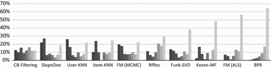
Distribution of recommendations (\(=\) being in the top-10 of a recommendation list) for all items sorted by popularity (number of ratings) and grouped into 8 bins with 120 items each (MovieLens400k dataset)
This observation also applies for FM (MCMC).
Compared to the sampling function shown in Fig. 12 for i, a corresponding function for j would have to be flipped horizontally.
Note that even after a 10 % drop with respect to recall (All), BPR would still be the best-performing technique in our comparison in Sect. 3.
Changing the rating prediction by small amounts is usually sufficient to push an item several places up in the recommendation lists.
While the absolute values can vary on each run even when the same data is used, the existence of the biases is not affected by the random initialization.

References
Adamopoulos, P., Tuzhilin, A.: On over-specialization and concentration bias of recommendations: probabilistic neighborhood selection in collaborative filtering systems. In: Proceedings of the 2014 ACM Conference on Recommender Systems (RecSys ’14), pp. 153–160, Foster City (2014a)
Adamopoulos, P.: Beyond rating prediction accuracy: on new perspectives in recommender systems. In: Proceedings of the 2013 ACM Conference on Recommender Systems (RecSys ’13), pp. 459–462. Hong Kong (2013)
Adamopoulos, P., Tuzhilin, A.: On unexpectedness in recommender systems: or how to better expect the unexpected. ACM Trans. Intell. Syst. Technol. 5(4), 54:1–54:32 (2014b)
Adomavicius, G., Kwon, Y.: Improving aggregate recommendation diversity using ranking-based techniques. IEEE Trans. Knowl. Data Eng. 24(5), 896–911 (2012)
Adomavicius, G., Tuzhilin, A.: Toward the next generation of recommender systems: a survey of the state-of-the-art and possible extensions. IEEE Trans. Knowl. Data Eng. 17(6), 734–749 (2005)
Adomavicius, G., Zhang, J.: Impact of data characteristics on recommender systems performance. ACM Trans. Manag. Inform. Syst. 3(1), 3:1–3:17 (2012)
Bradley, K., Smyth, B.: Improving recommendation diversity. In: Proceedings of the 12th National Conference in Artificial Intelligence and Cognitive Science (AICS ’01), pp. 75–84. Maynooth (2001)
Breese, J.S., Heckerman, D., Kadie, C.M.: Empirical analysis of predictive algorithms for collaborative filtering. In: Proceedings of the 14th Conference on Uncertainty in Artificial Intelligence, pp. 43–52. Madison (1998)
Celma, O., Herrera, P.: A new approach to evaluating novel recommendations. In: Proceedings of the 2008 ACM Conference on Recommender Systems (RecSys ’08), pp. 179–186. Lausanne (2008)
Chau, P.Y.K., Ho, S.Y., Ho, K.K.W., Yao, Y.: Examining the effects of malfunctioning personalized services on online users’ distrust and behaviors. Decision Support Syst. 56, 180–191 (2013)
Cremonesi, P., Koren, Y., Turrin, R.: Performance of recommender algorithms on top-n recommendation tasks. In: Proceedings of the 2010 ACM Conference on Recommender Systems (RecSys ’10), pp. 39–46. Barcelona (2010)
Cremonesi, P., Garzotto, F., Negro, S., Papadopoulos, A.V., Turrin, R.: Looking for ”good” recommendations: a comparative evaluation of recommender systems. In: Proceedings of the 13th International Conference on Human-Computer Interaction (INTERACT ’11), vol. 6948 of Lecture Notes in Computer Science, pp. 152–168. Lisbon. Springer, Berlin (2011)
Cremonesi, P., Garzotto, F., Turrin, R.: Investigating the persuasion potential of recommender systems from a quality perspective: an empirical study. ACM Trans Interact. Intell. Syst. 2(2), 11:1–11:41 (2012)
Cremonesi, P., Garzotto, F., Quadrana, M.: Evaluating top-n recommendations “when the best are gone”. In: Proceedings of the 2013 ACM Conference on Recommender Systems (RecSys ’13), pp. 339–342. Hong Kong (2013a)
Cremonesi, P., Garzotto, F., Turrin, R.: User-centric vs. system-centric evaluation of recommender systems. In: Proceedings of the 15th International Conference on Human-Computer Interaction (INTERACT ’13), vol. 8119 of Lecture Notes in Computer Science, pp. 334–351. Cape Town. Springer, Berlin (2013b)
Dias, M.B., Locher, D., Li, M., El-Deredy, W., Lisboa, P.J.: The value of personalised recommender systems to e-business: a case study. In: Proceedings of the 2008 ACM Conference on Recommender Systems (RecSys ’08), pp. 291–294. Lausanne (2008)
Ekstrand, M.D., Ludwig, M., Konstan, J.A., Riedl, J.T.: Rethinking the recommender research ecosystem: Reproducibility, openness, and LensKit. In: Proceedings of the 2011 ACM Conference on Recommender Systems (RecSys ’11), pp. 133–140. Chicago (2011)
Ekstrand, M.D., Harper, F.M., Willemsen, M.C., Konstan, J.A.: User perception of differences in recommender algorithms. In: Proceedings of the 2014 ACM Conference on Recommender Systems (RecSys ’14), pp. 161–168. Foster City (2014)
Fleder, D., Hosanagar, K.: Blockbuster culture’s next rise or fall: the impact of recommender systems on sales diversity. Manag. Sci. 55(5), 697–712 (2009)
Funk, S.: Netflix update: try this at home. http://sifter.org/~simon/journal/20061211.html (2006). Accessed June 2015
Gantner, Z., Rendle, S., Drumond, L., Freudenthaler, C.: MyMediaLite: example experiments. Results are published online at http://mymedialite.net/examples/datasets.html (2014). Accessed June 2015
Garcin, F., Faltings, B., Donatsch, O., Alazzawi, A., Bruttin, C., Huber, A.: Offline and online evaluation of news recommender systems at swissinfo.ch. In: Proceedings of the 2014 ACM Conference on Recommender Systems (RecSys ’14), pp. 169–176. Foster City (2014)
Ge, M., Jannach, D., Gedikli, F.: Bringing diversity to recommendation lists - an analysis of the placement of diverse items. In: Proceedings 14th International Conference on EnterpriseInformation Systems (ICEIS ’12), Springer Lecture Notes in Business Information Processing, vol. 141, pp. 293–305. Wrozlaw (2013)
Gedikli, F., Bagdat, F., Ge, M., Jannach, D.: Rf-rec: fast and accurate computation of recommendations based on rating frequencies. In: Proceedings of the 2011 IEEE 13th Conference on Commerce and Enterprise Computing (CEC ’11), pp. 50–57. Luxembourg (2011)
Herlocker, J.L., Konstan, J.A., Terveen, L.G., Riedl, J.T.: Evaluating collaborative filtering recommender systems. ACM Trans. Inform. Syst. 22(1), 5–53 (2004)
Jambor, T., Wang, J.: Optimizing multiple objectives in collaborative filtering. In: Proceedings of the 2010 ACM Conference on Recommender Systems (RecSys ’10), pp. 55–62. Barcelona (2010)
Jannach, D., Hegelich, K.: A case study on the effectiveness of recommendations in the mobile internet. In: Proceedings of the 2009 ACM Conference on Recommender Systems (RecSys ’09), pp. 205–208. New York (2009)
Jannach, D., Karakaya, Z., Gedikli, F.: Accuracy improvements for multi-criteria recommender systems. In: Proceedings of the 13th ACM Conference on Electronic Commerce (EC ’12), pp. 674–689. Valencia (2012a)
Jannach, D., Zanker, M., Ge, M., Gröning, M.: Recommender systems in computer science and information systems - a landscape of research. In: Proceedings 13th International Conference on E-Commerce and Web Technologies (EC-WEB ’12), pp. 76–87. Vienna (2012b)
Jannach, D., Lerche, L., Gedikli, F., Bonnin, G.: What recommenders recommend - an analysis of accuracy, popularity, and sales diversity effects. In: Proceedings of the 21st International Conference on User Modeling, Adaptation and Personalization (UMAP ’13), pp. 25–379. Rome (2013)
Javari, A., Jalili, M.: Accurate and novel recommendations: an algorithm based on popularity forecasting. ACM Transac. Intell. Syst. Technol. 5(4), 56:1–56:20 (2014)
Kirshenbaum, E., Forman, G., Dugan, M.: A live comparison of methods for personalized article recommendation at Forbes.com. In: Proceedings European Conference on Machine Learning and Knowledge Discovery in Databases (ECML/PKDD ’12), pp. 51–66. Bristol (2012)
Konstan, J.A., Riedl, J.: Recommender systems: from algorithms to user experience. User Model. User-Adapt. Interact. 22(1–2), 101–123 (2012)
Koren, Y.: Factorization meets the neighborhood: A multifaceted collaborative filtering model. In: Proceedings of the 14th ACM SIGKDD International Conference on Knowledge Discovery and Data Mining (KDD ’08), pp. 426–434. Las Vegas (2008)
Koren, Y.: Factor in the neighbors: scalable and accurate collaborative filtering. ACM Trans. Knowl. Discov. Data (TKDD) 4(1), 1:1–1:24 (2010)
Lee, J., Sun, M., Lebanon, G.: A comparative study of collaborative filtering algorithms. ACM Comput. Res. Repos., arxiv:1205.3193 (2012)
Lemire, D., Maclachlan, A.: Slope one predictors for online rating-based collaborative filtering. In: Proceedings of the SIAM Conference on Data Mining, pp. 471–480. Newport Beach (2005)
Linden, G., Smith, B., York, J.: Amazon.com recommendations: item-to-item collaborative filtering. IEEE Internet Comput. 7(1), 76–80 (2003)
McNee, S.M., Riedl, J., Konstan, J.A.: Being accurate is not enough: how accuracy metrics have hurt recommender systems. In: Proceedings of the 2006 Conference on Human Factors in Computing Systems (CHI ’06), pp. 1097–1101, Montreal (2006)
Murakami, T., Mori, K., Orihara, R.: Metrics for evaluating the serendipity of recommendation lists. In: Proceedings of the 2007 Conference on New Frontiers in Artificial Intelligence (JSAI ’07), pp. 40–46. Miyazaki (2008)
Niemann, K., Wolpers, M.: A new collaborative filtering approach for increasing the aggregate diversity of recommender systems. In: Proceedings of the 19th ACM SIGKDD International Conference on Knowledge Discovery and Data Mining (KDD ’13), pp. 955–963. Chicago (2013)
Pan, W., Zhong, H., Xu, C., Ming, Z.: Adaptive bayesian personalized ranking for heterogeneous implicit feedbacks. Knowledge-Based Syst. 73, 173–180 (2015)
Park, Y.-J., Tuzhilin, A.: The long tail of recommender systems and how to leverage it. In: Proceedings of the 2008 ACM Conference on Recommender Systems (RecSys ’08), pp. 11–18. Lausanne (2008)
Prawesh, S., Padmanabhan, B.: The “top N” news recommender: Count distortion and manipulation resistance. In: Proceedings of the 2011 ACM Conference on Recommender Systems (RecSys ’11), pp. 237–244. Chicago (2011)
Pu, P., Chen, L., Hu, R.: A user-centric evaluation framework for recommender systems. In: Proceedings of the 2011 ACM Conference on Recommender Systems (RecSys ’11), pp. 157–164. Chicago (2011)
Rendle, S., Freudenthaler, C., Gantner, Z., Schmidt-Thieme, L.: BPR: Bayesian personalized ranking from implicit feedback. In: Proceedings of the Twenty-Fifth Conference on Uncertainty in Artificial Intelligence (UAI ’09), pp. 452–461. Montreal (2009)
Rendle, S.: Factorization machines with libFM. ACM Trans. Intell. Syst. Technol. 3(3), 57:1–57:22 (2012)
Resnick, P., Iacovou, N., Suchak, M., Bergstrom, P., Riedl, J.: Grouplens: An open architecture for collaborative filtering of netnews. In: Proceedings of the 1994 ACM Conference on Computer Supported Cooperative Work (CSCW ’94), pp. 175–186. Chapel Hill (1994)
Said, A., Tikk, D., Stumpf, K., Shi, Y., Larson, M., Cremonesi, P.: Recommender systems evaluation: A 3D benchmark. In: Proceedings of the Workshop on Recommendation Utility Evaluation: Beyond RMSE (RUE ’12), pp. 21–23. Dublin. CEUR-WS Vol. 910 (2012)
Said, A., Bellogín, A., de Vries, A.: A top-n recommender system evaluation protocol inspired by deployed systems. In: ACM RecSys 2013 Workshop on Large-Scale Recommender Systems (LSRS ’13), Hong Kong (2013a)
Said, A., Fields, B., Jain, B.J., Albayrak, S.: User-centric evaluation of a k-furthest neighbor collaborative filtering recommender algorithm. In: Proceedings of the 2013 Conference on Computer Supported Cooperative Work (CSCW ’13), pp. 1399–1408. San Antonio (2013b)
Shani, G., Gunawardana, A.: Evaluating recommendation systems. In: Ricci, F., Rokach, L., Shapira, B., Kantor, P.B. (eds.) Recommender Systems Handbook, pp. 257–297. Springer, New York (2011)
Shi, Y., Karatzoglou, A., Baltrunas, L., Larson, M., Oliver, N., Hanjalic, A.: CLiMF: Learning to maximize reciprocal rank with collaborative less-is-more filtering. In: Proceedings of the 2012 ACM Conference on Recommender Systems (RecSys ’12), pp. 139–146. Dublin (2012)
Shi, L. Trading-off among accuracy, similarity, diversity, and long-tail: A graph-based recommendation approach. In: Proceedings of the 2013 ACM Conference on Recommender Systems (RecSys ’13), pp. 57–64. Hong Kong (2013)
Steck, H.: Item popularity and recommendation accuracy. In: Proceedings of the 2011 ACM Conference on Recommender Systems (RecSys ’11), pp. 125–132. Chicago (2011)
Vargas, S., Castells, P.: Rank and relevance in novelty and diversity metrics for recommender systems. In: Proceedings of the 2011 ACM Conference on Recommender Systems (RecSys ’11), pp. 109–116. Chicago (2011)
Zanker, M., Bricman, M., Gordea, S., Jannach, D., Jessenitschnig, M.: Persuasive online-selling in quality & taste domains. In: Proceedings of the 7th International Conference on Electronic Commerce and Web Technologies (EC-WEB ’06), pp. 51–60. Krakow (2006)
Zhang, M., Hurley, N.: Avoiding monotony: Improving the diversity of recommendation lists. In: Proceedings of the 2008 ACM Conference on Recommender Systems (RecSys ’08), pp. 123–130. Lausanne (2008)
Zhang, M., Hurley, N.: Niche product retrieval in top-n recommendation. In: Proceedings of the 2010 IEEE/WIC/ACM International Conference on Web Intelligence and Intelligent Agent Technology (WI-IAT ’10), pp. 74–81. Toronto (2010)
Zhang, Y. C., Séaghdha, D. Ó., Quercia, D., Jambor, T.: Auralist: Introducing serendipity into music recommendation. In: Proceedings of the Fifth ACM International Conference on Web Search and Data Mining (WSDM ’12), pp. 13–22. Seattle (2012)
Zhang, N., Zhang, Y., Tang, J.: A tag recommendation system for folksonomy. In: Proceedings of the 2nd Workshop on Social Web Search and Mining (SWSM ’09), pp. 9–16, Hong Kong (2009)
Zhang, M.: Enhancing the diversity of collaborative filtering recommender systems. PhD thesis, University College Dublin (2010)
Zhou, T., Kuscsik, Z., Liu, J.-G., Medo, M., Wakeling, J.R., Zhang, Y.-C.: Solving the apparent diversity-accuracy dilemma of recommender systems. Proc. National Acad. Sci. 107(10), 4511–4515 (2010)
Ziegler, C.-N., McNee, S.M., Konstan, J.A., Lausen, G.: Improving recommendation lists through topic diversification. In: Proceedings of the 14th International Conference on World Wide Web (WWW ’05), pp. 22–32. Chiba (2005)
Author information
Authors and Affiliations
Corresponding author
Appendix
Appendix
1.1 Gini index
The Gini index can be derived from the Lorenz curve, which is a cumulative distribution function as shown in Fig. 17. The diagonal corresponds to an even distribution. The higher the deviation of the Lorenz curve from the diagonal, the stronger is the unevenness of the distribution. The Gini index measures the strength of the inequality of a distribution and can be calculated as twice the difference between the area below the diagonal and the area below the curve (Zhang 2010).

An example of a Lorenz curve. The Gini index is proportional to the area between the diagonal and the curve
In our application setting, we calculate how often each item was included in a top-10 list, sort the items according to their popularity in increasing order and group them into n bins \(x_1, ..., x_n\), each containing 30 items.
For such a discrete distribution, the Gini index G can be computed using the formula
where \(p_n\) is the cumulative sum of the first n bins, i.e.,
With \(q_n\), we weight each \(x_i\) according to its rank position, i.e.,
To normalize G, we divide it by \(G_{max} = 1-(1/n)\) to finally obtain \(G_{norm}\)
1.2 Results for other datasets
Table 11 reports statistics for the datasets used in our evaluations. Tables 12, 13, 14, 15, 16, 17 and 18 show the corresponding results for the evaluated metrics (notation: P10T = Precision@10 (TS), R10A = Recall@10 (All), etc.). Furthermore AvgR denotes the average rating and AvgP the average popularity of the top-10 recommended items. Div is the diversity in terms of inverse ILS and NbRec the overall number of different items recommended by the algorithms. In each column, the highest value is highlighted in case the observed difference is statistically significant (p \(<\) 0.05) when compared to the other algorithms. Due to its high computational complexity, we did not test the user-KNN method for the 7 million Netflix and 1 million MovieLens dataset. The content-based algorithm could only be benchmarked on datasets for which content information was available.
1.3 Artificial popularity on other datasets
Tables 19, 20 and 21 show the results of the artificial popularity bias experiment (see Sect. 4.2) for the three datasets MovieLens400k, MovieLens1M and Yahoo!Movies on the precision and recall strategies All (all items in the test set) and TS (only items with known ratings in the test set). The algorithm only recommends items that were rated by at least p users in the training set.
1.4 Detailed results for the PBA algorithm
Tables 22 and 23 show the detailed results for the PBA method when applied to the output of Koren-MF and FM (ALS) respectively. As before the table headers are shortened (P10T = Precision@10 (TS), etc.). Furthermore AvgP denotes the average popularity of the top-10 recommended items and NbRec the overall number of different recommendations. The column \(\lambda \) shows which value was used for the regularization variable to produce the results in the corresponding row. The first row (with the \(\lambda \) value left blank) contains the raw output of the underlying algorithm unaltered by the PBA method.
1.5 Partial derivatives for the PBA algorithm
To minimize the optimization goal of the PBA algorithm (see Eq. 8) via a gradient descent strategy we have to calculate the partial derivatives of the minimization function to estimate the step width. The derivative for a specific \(x_{ui}\) can be calculated as follows:
with the first part being reducible in the following way
and the latter part being reducible to
Thus, the combined derivatives form the following assignment rule for each gradient descent step:
Rights and permissions
About this article

Cite this article
Jannach, D., Lerche, L., Kamehkhosh, I. et al. What recommenders recommend: an analysis of recommendation biases and possible countermeasures. User Model User-Adap Inter 25, 427–491 (2015). https://doi.org/10.1007/s11257-015-9165-3
Received:
Accepted:
Published:
Issue Date:
DOI: https://doi.org/10.1007/s11257-015-9165-3