
Abstract
It has been argued recently (Beall in Spandrels of truth, Oxford University Press, Oxford, 2009; Beall and Murzi J Philos 110:143–165, 2013) that dialetheist theories are unable to express the concept of naive validity. In this paper, we will show that \(\mathbf {LP}\) can be non-trivially expanded with a naive validity predicate. The resulting theory, \(\mathbf {LP}^{\mathbf {Val}}\) reaches this goal by adopting a weak self-referential procedure. We show that \(\mathbf {LP}^{\mathbf {Val}}\) is sound and complete with respect to the three-sided sequent calculus \(\mathbf {SLP}^{\mathbf {Val}}\). Moreover, \(\mathbf {LP}^{\mathbf {Val}}\) can be safely expanded with a transparent truth predicate. We will also present an alternative theory \(\mathbf {LP}^{\mathbf {Val}^{*}}\), which includes a non-deterministic validity predicate.
1 Introduction
Dialetheists argue that the acceptance of contradictions is the best way to solve the paradoxes while achieving a semantically closed language. In recent years, Beall (2009) and Beall and Murzi (2013) tried to show that dialetheism is unable to express the concept of naive validity. The inexpressibility result goes as follows.
Let \(\mathbf {Val}\) be a \(\mathbf {naive}\) validity predicate, characterized by the following rules and meta-rules. Let A and B be formulas variables. \(\langle A \rangle \) and \(\langle B \rangle \) are names for A and B, respectively. The so-called naive validity principles are the following:

If the theory achieves self-reference through something like strong diagonalization, there will be a sentence A definitionally equivalent to \(\textit{Val}(\langle A \rangle , \langle \bot \rangle )\), usually known as “the Beall–Murzi sentence.” This sentence will cause major harm, as the following proof shows.

The proof is carried out in a sequent system that has Contraction as a valid meta-rule.Footnote 1 The dialetheist, then, should give up some of the principles involved in the proof. She must abandon \(\textit{VD}\) (the initial sequent is an instance of it), \(\textit{VP}\), \(\textit{MetaVD}\), the inter-sustitutivity of \({ Val}(\langle A \rangle , \langle \bot \rangle )\) and A or Contraction. Rejecting Contraction seems not a natural option, at least if the dialetheist supports \({ LP}\) or the non-transitive logic ST. But the rest of them are still suspects. As the supporters of ST must reject \(\textit{MetaVD}\), and we are trying to find out if a dialetheist approach is compatible with a naive validity predicate, we will focus on what a supporter of \({ LP}\) should do in a case like this. We will argue that she can internalize a naive validity predicate. To do that, she must change the way to achieve self-reference. In particular, she must move from (what we will call) a strong self-referential procedure to a weak one. Thus, Def. Eq., the principle that establishes that we can substitute “the Beall–Murzi sentence” for another sentence identical to it, must be dropped. Self-reference will be obtained instead through a suitable biconditional, e.g., a conjunction of conditionals. Those constants will be instances of \({ LP}\)’s material conditional, which does not validates Modus Ponens. In Goodship (1996), Laura Goodship provides a general remark regarding the alternatives for this biconditional. If we want the theory to be safe from trivialization due to semantic paradoxes, there seem to be two main routes: (1) either the conditional should invalidate Modus Ponens, or (2) it should invalidate Contraction and Pseudo Modus Ponens. In this paper, we will explore one possible realization of the first alternativeFootnote 2: we will consider a theory of naïve validity that invalidates Modus Ponens since it is based on the paraconsistent logic LP. The paper is structured as follows. In Sect. 2 we present the dialetheist logic \(\mathbf {LP}\), the semantic notion of \(\mathbf {validity}\) that an LP’s supporter may wish to internalize and show that it is a \(\mathbf {naive}\) one. In Sect. 3 we demonstrate how to extend \(\mathbf {LP}\) with a naive validity predicate. We will call the resulting theory \(\mathbf {LP}^{\mathbf {Val}}\). \(\mathbf {LP}^{\mathbf {Val}}\) uses a weak self-referential procedure. We will show that it is non-trivial. Therefore, Beall and Murzi were wrong in claiming that a dialetheist theory cannot be expanded with a \(\mathbf {naive}\) validity predicate. We will also give a three-sided sequent calculus for \(\mathbf {LP}^{\mathbf {Val}}\), \(\mathbf {SLP}^{\mathbf {Val}}\), and show that it is sound and complete with respect to \(\mathbf {LP}^{\mathbf {Val}}\). In Sect. 4, we will demonstrate how to add a transparent truth predicate to \(\mathbf {LP}^{\mathbf {Val}}\). In Sect. 5, we will present an objection raised against this approach, and developed an alternative theory with a non-deterministic and naive validity predicate. Finally, in Sect. 6 we make some concluding remarks. Completeness proofs for both \(\mathbf {SLP}^{\mathbf {Val}}\) and \(\mathbf {SLP^{Val+}}\) can be found in the “Appendix”.
2 Two ways to achieve self-reference in a dialetheist theory of validity
Graham Priest’s \(\mathbf {LP}\) is a first order logic, with the usual connectives (negation, conjunction, etc) and a standard three-valued (\(1, \frac{1}{2}, 0\)) Strong Kleene interpretation.Footnote 3 For the sake of simplicity, we will deal with a propositional version of \(\mathbf {LP}\). We show below the matrices for \(\mathbf {LP}\)’s connectives. Validity is understood in the usual way, as the preservation of designated values. \(\mathbf {LP}\)’s designated values are \(1, \frac{1}{2}\) (Fig. 1).

Matrices for the logic \(\mathbf {LP}\)
Our goal, then, is to internalize the notion of naive validity. One way to do it is by adding a naive validity predicate to \({ LP}\)’s language.Footnote 4 We will need, then, both (i) a way to name the sentences of the language, and also (ii) a way to build self-referential sentences. To achieve (i), we will introduce designated names for every sentence. Thus, for every sentence A, \(\langle A \rangle \) will be the name of A in every model. Though this can also help us achieve (ii), it is not necessary nor desirable, as we will see soon. But before that, we need to examine carefully the two main options we have. Either way, they should let us have in the language potentially problematic or pathological formulas, like the Beall–Murzi sentence that allegedly causes trouble to dialetheism.
Probably the most popular and common way to build self-referential sentences is through \(\mathbf {PA}\), first-order Peano Arithmetic. In \(\mathbf {PA}\), self-reference is usually taken to be achieved through the weak and/or the strong Diagonal Lemma.Footnote 5 According to (a simplified version of) the Weak Diagonal Lemma, for each open formula \(\phi (x)\), there is a formula \(\psi \) such that the theory proves that \(\phi (\langle \psi \rangle )\) is equivalent to \(\psi \). But one may want more. In particular, one may search for linguistic items that are identical to other linguistic items that talk about the first ones. The Strong Diagonal Lemma is usually interpreted as a way to get precisely that, through names that refer to sentences that include that same name as one of its terms.
There seem to be two main options to represent self-reference in a theory: either through a weak or a strong procedure. The former achieves this goal by requiring a self-referential sentence to be equivalent to a sentence that “talks about” the first one. The latter involves an essential use of identities.
We will present general versions of both the weak and the strong procedures. These principles may be understood, on the one hand, as semantic versions of proof-theoretic self-referential principles, and, on the other hand, as general procedures that are instantiated (in \(\mathbf {PA}\)) by the (semantic versions of the) Weak and the Strong Diagonal Lemma.Footnote 6
These options might be instantiated by a plethora of technical tools, varying from one framework to the other. In this paper, we will discuss some examples thereof.
Definition 2.1
(Weak Self-Referential Procedure) Let \(\mathbf {Th}\) be a theory that has a name-forming device \(\langle \cdot \rangle \). If for every formula A(x), with x as the only free variable in A(x), there is a (closed) formula B such that the formula \(B \leftrightarrow A(\langle B \rangle )\) is true in \(\mathbf {Th}\), then we say that \(\mathbf {Th}\) adopts a weak self-referential procedure.
Definition 2.2
(Strong Self-Referential Procedure) Let \(\mathbf {Th}\) be a theory that has a name-forming device \(\langle \cdot \rangle \). If for every formula A(x), with x as the only free variable, there is a term t such that t is identical to the name of A(t) in \(\mathbf {Th}\), then we say that \(\mathbf {Th}\) adopts a strong self-referential procedure.
Remark 2.3
Notice that these procedures can sometimes be already present “in” the theories in question, e.g. if they are extensions of arithmetical theories that validate the Weak and/or the Strong Diagonal Lemma. But in some cases, they do not come with the theories, but are “imposed from the meta-language”, e.g. by restricting the valuations to the ones that guarantee that the relevant biconditionals take a designated value.
Moreover, it is possible for a theory to satisfy one procedure, but not the other. For example, if one works with a language that does not have an identity operator, or one does not adopt a meta-linguistic function from names to formulas that restrict the models, then the theory lacks the resources to have a Strong Self-Referential Procedure. Nevertheless, the theory may include a Weak Self-Referential Procedure. We will see below an example of such a theory.Footnote 7
Let’s now return to what was our initial goal: to add a naive validity predicate Val to LP. Val, then, must satisfy \(\textit{VD}\), \(\textit{VP}\) and \(\textit{MetaVD}\). Suppose that a strong self-referential procedure is added to the expanded \(\mathcal {LP}\). There seems to be one big problem with this way of doing things: the theory becomes trivial. And this is because, as we are using a strong self-referential procedure, there will be some name \(\langle B \rangle \) such that \(\langle B \rangle = \langle \textit{Val}(\langle B \rangle , \langle \perp \rangle \rangle )\). And as \({ Val}\) satisfies \(\textit{VD}\), \(\textit{VP}\) and \(\textit{MetaVD}\), and the consequence relation is contractive, then we may reason as we do on page 2 and go on to prove \(\perp \).
Moreover, if the theory allows some strong self-referential procedure like strong diagonalization, there will be a sentence A definitionally equivalent to \({ Val}(\langle A \rangle , \langle \bot \rangle )\), e.g. “the Beall–Murzi sentence.” Now reason as follows.Footnote 8

The first step is an instance of \(\textit{VD}\). Remember that \(\langle A \rangle \) is a name of \({ Val}(\langle A \rangle , \langle \bot \rangle )\). This also explains why the second inferential step is a case of \(\textit{VP}\).
A similar reasoning will prove another instance of \(\vdash Val(\langle A \rangle , \langle \bot \rangle )\). A further application of \(\textit{MetaVD}\) will prove \(\bot \). And as for any formula B, \(\bot \vdash B\), an application of \(\textit{VP}\) will prove \(\vdash \textit{Val}(\langle \bot \rangle , \langle B \rangle )\). Then, an application of \(\textit{MetaVD}\) will show that \(\vdash B\).
Our initial goal was to find a way to expand \({ LP}\) with a naive validity predicate. We will explore another way to achieve this aim. It will involve a radical change in the self-referential procedure adopted. As we have shown, it cannot be a strong one. We will use instead a weak self-referential procedure, as we will see in the next section.
3 Weak self-reference for \(\mathbf {LP}^{\mathbf {Val}}\)
We will now present a weak self-referential procedure for \({ LP}\). We will show how this makes possible to expand \({ LP}\) with a naive validity predicate \({ Val}\) in a way that avoids triviality. It is important to remark that there may be many other ways to achieve this goal, and this is just one option. We will now give a formal presentation of the target theory, \(\mathbf {LP}^{\mathbf {Val}}\).
\(\mathbf {LP}^{\mathbf {Val}}\) will be the result of expanding (the propositional version of) \(\mathbf {LP}\) with infinitely many names for every formula in the language, and a validity predicate \({ Val}\). \({ Val}\) will be defined by the following matrix (Fig. 2).

Matrix for Val
This matrix is a natural one for an \(\mathbf {LP}\)naive validity predicate.Footnote 9 It reflects \(\mathbf {LP}\)’s consequence relation, as it gets value 1 iff (designated) values \(1, \frac{1}{2}\) are preserved from premises—represented by the first term of the assertion—to conclusion—represented by the the second term. Moreover, it reflects the fact that there are no validity “gaps” or “gluts”—e.g. there is no inference that is neither (both) valid nor (and) invalid.Footnote 10
Despite being a natural matrix for a validity predicate for \({ LP}\), this is not the only one that can be suitable for it. The only restriction that has been imposed to those possible candidates is that they should satisfy \(\textit{VD}\), \(\textit{VP}\) and \(\textit{MetaVD}\). And this can be achieved in multiple ways. For example, one can specify a new validity predicate \({ Val}_{1}\) such that \(v({ Val}_1(\langle \gamma _1 \wedge \ldots \wedge \gamma _n \rangle , \langle \phi \rangle )) = \frac{1}{2}\) iff either \(v(\gamma _1 \wedge \ldots \wedge \gamma _n) = \frac{1}{2}\) or \(v(\phi ) = \frac{1}{2}\), or if just \(v(\gamma _1 \wedge \ldots , \gamma _n) = \frac{1}{2}\) or \(v(\phi ) = \frac{1}{2}\), but not if both get that value. In fact, one can safely add at once all those predicates associated with different “validity-related” matrices, as long as a weak self-referential procedure is adopted.Footnote 11 Thus, we should turn to that issue now.
3.1 Technical details
To guarantee non-triviality we will use a weak self-referential procedure. As we are working in a semantic framework that does not extend \(\mathbf {PA}\), we need to find some other way to validate the Weak Self-Referential Principle. This will require that statements that fix the self-referential character of the target sentences should be true in our theory, e.g. they should get a designated value in every relevant valuation. We will accomplish this task by restricting the set of valuations to the ones that guarantee this result. Moreover, we will also need to make some other minor adjustments.
First, we need to select an infinite proper subset of propositional variables. We will mark them—in the metalanguage—with an \(^{*}\).Footnote 12 Let’s consider, then, the sentence-scheme \(x^{*} \leftrightarrow A_{x^{*}}\), where \(A_{x^{*}}\) is any sentence that has at least one instance of \({ Val}(\langle x^{P} \rangle , \langle x^{C} \rangle )\) as a subformula, and \(x^{*}\) is a distinguished propositional letter. \({ Val}(\langle x^{P} \rangle , \langle x^{C} \rangle )\) will be a validity assertion such that \(x^{*}\) is a subformula of either \(x^{P}\), \(x^{C}\), or of both of them. Finally, for every formula C, \(\langle C \rangle \) will be a designated name for C, built with the help of a function symbol Q that will be added to the language, such that \(Q(C) = \langle C \rangle \). The instances of \(A_{x^{*}}\) in the biconditional statement will give us every potential self-referential sentence that includes a validity predicate that can be represented in the language.Footnote 13
Thus, we will be able to model the pathological sentences that will be around when predicates like \({ Val}(x, y)\) are added to the language. In particular, we will have in the language sentences like \(p^{*} \leftrightarrow \textit{Val}(\langle p^{*} \rangle , \langle r \rangle )\) or \(q^{*} \leftrightarrow \lnot \textit{Val}(\langle (\lnot s \rangle , \langle q^{*} \rangle )\). We will impose a further semantic restriction to this setting. Let y be a metalinguistic variable that ranges over propositional letters, and let B be also a metalinguistic variable that ranges over formulas that include at least one instance of \({ Val}(\langle y^{P} \rangle , \langle y^{C} \rangle )\). A formula-scheme \(B_{y}\) will be an instantiation of B, e.g., a formula such that every expression in it (besides parenthesis) is either a propositional letter, or a logical constant, or the metalinguistic variable y. Therefore, \({ Val}(\langle p^{*} \rangle , \langle r \rangle )\) and \({ Val}(\langle q \rangle , \langle p^{*} \rangle )\) are different formula-schemes.
We will select, for each formula-schema \(B_{y}\), one and only one biconditional. Each one of them will have a different distinguished propositional letter as its left term. Let Z be the set of such biconditionals.
Finally, we will restrict the valuations to the ones that assign a designated value to each member of Z.Footnote 14 This makes those biconditionals true in every valuation, and allows a version of the Weak Self-Referential Principle to hold in the target theory, \(\mathbf {LP}^{\mathbf {Val}}\).Footnote 15 Thus, though every member of Z will be an instance of the Weak Self-Referential Principle, not every instance of the Weak Self-Referential Principle will be a member of Z. For example, if \(p^{*} \leftrightarrow Val(\langle p^{*} \rangle , \langle r \rangle )\) is a member of Z, then, \(q^{*} \leftrightarrow \textit{Val}(\langle q^{*} \rangle , \langle r \rangle )\), is not.Footnote 16
It is essential that we use a biconditional to represent self-referential sentences that receives value 0 only when the antecedent receives value 1 and the consequent receives value 0, and that receives value \(\frac{1}{2}\) when the antecedent receives value \(\frac{1}{2}\) and the consequent value 0. \({ LP}\)’s material biconditional belongs to that group.
The following fact about \(\mathbf {LP}^{\mathbf {Val}}\) must be highlighted: it is a non-trivial theory.
Theorem 3.1
(Non-triviality) There is at least one valuation that does not give a designated value to every formula of \(\mathbf {LP}^{\mathbf {Val}}\).
Proof
Take a valuation v that assigns \(\frac{1}{2}\) to every propositional letter. Let \(p^{*}\) be the propositional letter of the Beall–Murzi biconditional for \(\mathbf {LP}^{\mathbf {Val}}\), \(p^{*} \leftrightarrow \textit{Val}(\langle p^{*} \rangle , \langle \perp \rangle )\). Thus, \(v(p^{*}) = \frac{1}{2}\). (In fact, that is the only value that \(p^{*}\) can receive in any valuation.) Now consider the validity assertion \({ Val}(\langle p^{*} \rangle , \langle p^{*} \rangle )\). As is easy to check, v will be such that \(v({ Val}(\langle p^{*} \rangle , \langle p^{*} \rangle )) = 1\). Therefore, \(v(\lnot Val(\langle p^{*} \rangle , \langle p^{*} \rangle )) = 0\). Thus, \(\mathbf {LP}^{\mathbf {Val}}\) is not trivial. The only thing we need to check is if v is an admissible valuation—e.g. a valuation that gives a designated value to every biconditional in Z. But, as we have established, every propositional letter q will be such that \(v(q) = \frac{1}{2}\), including every propositional letter distinguished with a \(*\). Thus, every biconditional \(r^{*} \leftrightarrow A_{r^{*}}\) that belongs to Z will receive a designated value in v.Footnote 17\(\square \)
So far, we have proved that \(\mathbf {LP}\) can be expanded with the predicate Val. Nevertheless, we still need to prove that Val expresses \(\textit{naive}\) validity.
Theorem 3.2
(Val is a naive validity predicate).
Proof
\(\textit{Val}\) satisfies the semantic versions of \(\textit{VP}\), \(\textit{VD}\) and \(\textit{MetaVD}\).
In the cases of \(\textit{VP}\) and \(\textit{MetaVD}\), this means that those rules are validity-preserving: if the premises are valid, then the conclusion is valid too. In the case of \(\textit{VD}\), it means that it is a valid inference. Let’s start with \(\textit{VP}\). If \( A \vDash B\), then, for every valuation v, either \(v(A) = 0\) or \(v(B) \in \{1, \frac{1}{2} \}\). In either case, \(v({ Val}(\langle A \rangle , \langle B \rangle ) = 1\). Now we need to prove the semantic version of \(\textit{VD}\): \(A, Val(\langle A \rangle , \langle B) \rangle \vDash B\). If the premises are true in a valuation v, then either \(v(A) = 0\) or \(v({ Val}(\langle A \rangle , \langle B \rangle ) = 0\), or, if v(A), \(v({ Val}(\langle A \rangle , \langle B \rangle ) \in \{1, \frac{1}{2} \}\), then \(v(B) \in \{1, \frac{1}{2} \}\). The only relevant case is the one where v(A), \(v({ Val}(\langle A \rangle , \langle B \rangle ) \in \{1, \frac{1}{2} \}\). But in that case, by the matrix corresponding to \({ Val}\), \(v(B) \in \{1, \frac{1}{2} \}\), and so we are done. If \(\textit{MetaVD}\) is a valid (meta)rule, if both \(\vDash \textit{Val}(\langle A \rangle , \langle B \rangle ) \) and \(\vDash A\), then, once again by \({ Val}\)’s matrix, \(\vDash B\). \(\square \)
Thus, we have proven that \(\mathbf {LP}^{\mathbf {Val}}\) can internalize a \(\textit{naive}\) validity predicate. But it may be claimed that all we have proven is that it can internalize semantic versions of the principles that a real \(\textit{naive}\) validity predicate should satisfy. And to prove what we intended to prove, we need to present a calculus that is sound and complete with respect to \(\mathbf {LP}^{\mathbf {Val}}\).
That is what we will do in the next section.
3.2 A sequent calculus for \(\mathbf {LP}^{\mathbf {Val}}\)
We will now present the three-sided disjunctive sequent system \(\mathbf {SLP}^{\mathbf {Val}}\) (for “Sequent system for \(\mathbf {LP}^{\mathbf {Val}}\)”). We are not claiming that it is impossible to give a traditional, two-sided sequent calculus, but the three-sided calculus that we will display simplifies the completeness proof given in the “Appendix”. Moreover, \(\mathbf {SLP}^{\mathbf {Val}}\) has two further advantages. On the one hand, each truth value will be represented in it, something that a two-sided sequent system cannot obviously do. On the other hand, \(\mathbf {SLP}^{\mathbf {Val}}\) makes it easy to realize what is special about pathological sentences like the Beall–Murzi sentence. Those sentences cannot receive a classical truth value in any valuation.Footnote 18
We will now specify how disjunctive sequents behave. \( \Gamma , \Sigma , \Delta \) will be sets of sentences.
Definition 3.3
A disjunctive sequent \( \Gamma \mid \Sigma \mid \Delta \) is satisfied by a valuation v iff \(v(\gamma )=0\) for some \(\gamma \in \Gamma \), or \(v(\sigma )= \frac{1}{2}\) for some \(\sigma \in \Sigma \), or \(v(\delta )=1\) for some \(\delta \in \Delta \). A sequent is valid iff it is satisfied by every valuation. A valuation v is a counterexample to a sequent if v does not satisfy the sequent.
An inference from \(\Gamma \) to \(\Delta \) will be valid in \(\mathbf {LP}^{\mathbf {Val}}\) if and only if there is no valuation such that every formula in \(\Gamma \) receives a value 1, \(\frac{1}{2}\) and every formula in \(\Delta \) receives value 0. There is a strong relation between valid three-sided sequents and valid \(\mathbf {LP}^{\mathbf {Val}}\)’s inferences:
This follows from the definition of \(\mathbf {LP}^{\mathbf {Val}}\) validity and the definition of validity for a three-sided sequent.
The proof system we are about to present includes, as usual, some axioms and rules. A sequent is provable if and only if it follows from the axioms by some number (possibly zero) of applications of the rules. As we are working with sets, the effects of Exchange and Contraction are built in, and Weakening is built into the axioms. \(\mathbf {LP}^{\mathbf {Val}}\) has three forms of Cut, and also a Derived Cut rule (that can be inferred from the three basic rules of Cut) that will play a key part in the Completeness Proof. Id, SeudoDL (short for “Seudo Diagonal Lemma”) and VAL are the axiom-schemes of \(\mathbf {SLP}^{\mathbf {Val}}\).Footnote 19\(Cut_1\), \(Cut_2\), \(Cut_3\) and DerivedCut are structural rules. The rest of them are \(\mathbf {SLP}^{\mathbf {Val}}\)’s operational rules. To apply the rule SeudoDL, \(p^{*} \leftrightarrow A_{p^{*}}\) must be a member of Z.

As the rest of the constants (\(\vee \), \(\rightarrow \) and \(\leftrightarrow \)) can be defined in terms of the former, we will not specify rules for them.
The following are some important properties of \(\mathbf {LP}^{\mathbf {Val}}\) and \(\mathbf {SLP}^{\mathbf {Val}}\):
Theorem 3.4
(Soundness) If a sequent \(\Gamma \mid \Sigma \mid \Delta \) is provable, then it is valid.
Proof
The axioms are valid, and validity is preserved by the rules, as can be checked without too much trouble. \(\square \)
Theorem 3.5
(Completeness) If a sequent \(\Gamma \mid \Sigma \mid \Delta \) is valid, then it is provable.
Proof
In the “Appendix”. \(\square \)
4 Adding a transparent truth predicate
So far, we have shown how to expand the dialetheist logic \(\mathbf {LP}\) with a naive validity predicate that also expresses its own notion of semantic consequence. There are several validity theories that intend to solve the Validity Paradox in a variety of ways. But a promising theory of validity that is immune to semantic paradoxes should also interact safely with a transparent truth predicate.Footnote 20 This is what we will get with \(\mathbf {LP}^{\mathbf {Val+}}\). \(\mathbf {LP}^{\mathbf {Val+}}\) expands \(\mathbf {LP}^{\mathbf {Val}}\)’s language with a transparent truth predicate \({ Tr}\) (Fig. 3).

Matrix for Tr
One important thing about \(\mathbf {LP}^{\mathbf {Val+}}\) is that its weak self-referential procedure should be slightly different from the one we saw for it to allow not only self-referential sentences involving the validity predicate, but also self-referential sentences involving the truth predicate or both of them. Thus, we will have new self-referential sentences as terms of the biconditionals used to express self-reference. Those biconditionals will have, as theirs right terms, formulas that include instances of Tr. Sentences of the form \(x^{*} \leftrightarrow A_{x^{*}}\) will now be understood as formulas where \(A_{x^{*}}\) refers to a sentence that with least one instance of \({ Val}(\langle x^{P} \rangle , \langle x^{C} \rangle )\) or at least one instance of \({ Tr}(\langle x^{*} \rangle )\) as subformulas.
Now we can model the pathological sentences that are around when predicates like validity or truth are introduced in the language. Once again, we will select, for each formula-schema \(A_{x^{*}}\), one and only one biconditional. Each biconditional will have a different propositional letter as its left term. We will call our new set of such biconditionals, \(Z*\).
The valuations will be restricted to the ones that assign a designated value to each member of \(Z*\).Footnote 21 This allows a version of the Weak Self-Referential Principle to hold in our theory, as those biconditionals will become true in every valuation.
Theorem 4.1
(Non-triviality) There is at least one valuation v such that for some formula A of \(\mathbf {LP}^{\mathbf {Val}}\), \(v(A)=0\).
Proof
The same strategy as the one used to prove \(\mathbf {LP}^{\mathbf {Val}}\)’s non-triviality can be used to prove that \(\mathbf {LP}^{\mathbf {Val+}}\) is not trivial. \(\square \)
\(\mathbf {LP}^{\mathbf {Val+}}\) will be sound and complete with respect to a new disjunctive three-sided sequent system, \(\mathbf {SLP}^{\mathbf {Val+}}\). \(\mathbf {SLP}^{\mathbf {Val+}}\) expands \(\mathbf {SLP}^{\mathbf {Val}}\) with a transparent truth predicate, and three new rules for it.

To apply SeudoDL, \(p^{*} \leftrightarrow A_{p^{*}}\) must be a member of \(Z*\).
The relation between valid sequents of \(\mathbf {SLP}^{\mathbf {Val+}}\) and valid inferences of \(\mathbf {LP}^{\mathbf {Val+}}\) will be once more the expected one. Moreover, \(\mathbf {SLP}^{\mathbf {Val+}}\) is sound and complete with respect to \(\mathbf {LP}^{\mathbf {Val+}}\).
Theorem 4.2
(Soundness) If a sequent \(\Gamma \mid \Sigma \mid \Delta \) (of \(\mathbf {SLP}^{\mathbf {Val+}}\)) is provable, then it is valid.
Proof
The axioms are valid, and validity is preserved by the rules, as can be easily checked. \(\square \)
Theorem 4.3
(Completeness) If a sequent \(\Gamma \mid \Sigma \mid \Delta \) (where each sentence in the sequent is a \(\mathbf {LP}^{\mathbf {Val+}}\)’s formula) is valid, then it is provable in \(\mathbf {SLP}^{\mathbf {Val+}}\).
Proof
In the “Appendix”. \(\square \)
5 Validity as an intensional notion
We will like to mention one important objection against this approach raised by Graham Priest. Validity is an intensional notion. It cannot be modeled by a matrix, because the resulting theory will be deeply unsound: it will make true validity assertions that are not intuitively valid.Footnote 22 Take a valuation v such that \(v(p)=1\) and \(v(q)=0\). Then \(v({ Val}(\langle q \rangle , \langle p \rangle ))=1\). But this surely isn’t right, because p and q are independent contingent formulas.
It is important to understand that this argument doesn’t tell against treating a validity predicate as a sort of conditional, but against interpreting it as a deterministic, extensional connective, whose meaning is fixed by its truth-table. Every validity predicate resembles a kind of conditional. One of the main features of a semantically closed theory is to have a way to express in the theory its consequence relation. And the linguistic item that fulfills this task will be relating the premises and conclusions in very much the same way as a suitable conditional \(\rightarrow \) will relate the antecedent and the consequent. Let \(\gamma _1, \ldots , \gamma _n\) be the formulas in \(\Gamma \). The validity predicate and such a conditional should satisfy both the Deduction Theorem and its converse:
\(\Gamma \vDash \phi \) iff \(\vDash \textit{Val}(\langle \Gamma \rangle , \langle \phi \rangle )\)
\(\Gamma \vDash \phi \) iff \(\vDash (\gamma _1 \wedge \ldots \wedge \gamma _n) \rightarrow \phi \)
Thus, the problem seems not to be that we model validity with a conditional, but that we use a deterministic conditional. If the validity predicate is associated with a particular deterministic matrix, then its truth-value will be fixed by the values of its terms. But of course, the truth of a validity assertion in a particular valuation v does not imply that that validity assertion is true in the theory. To be true in the theory, it should be true in every valuation. And it is not that awkward to say that those assertions are valid, or true in (or according to) the theory. Thus, even if those valuations make true sentences like \({ Val}(\langle q \rangle , \langle p \rangle )\), it is not the case that they will be valid, or true in the theory.Footnote 23
Moreover, it is not even true that validity is necessarily associated with “necessary truth-preservation”, or some other related notion. From an inferentialist perspective, to capture a notion like validity in the language, is to add a symbol to the language, and, moreover, rules that express its normative use in the inferential practice. Most probably, an inferentialist will consider \(\textit{VP}\), \(\textit{VD}\), and maybe \(\textit{MetaVD}\), as the rules that capture the meaning of the validity predicate.Footnote 24 From the inferentialist’s perspective, there is nothing essential about validity that a predicate does not capture if it obeys those rules. Thus, an inferentialist that recognizes \(\textit{VP}\), \(\textit{VD}\) and \(\textit{MetaVD}\) as the rules that define a validity predicate will accept \({ Val}\) as a full-blooded validity predicate.
Nevertheless, there may be inferentislists that think that the anti-extensionalist argument we presented before is sound. Thus, if validity cannot be modelled by a traditional, deterministic matrix, but nevertheless it should satisfy \(\textit{VP}\), \(\textit{VD}\) and \(\textit{MetaVD}\), then it should be inferred that some naive validity predicates, such as \({ Val}\), are not real validity predicates. The mistake, then, is to think that \(\textit{VP}\), \(\textit{VD}\) and \(\textit{MetaVD}\) are not only necessary, but also (jointly) sufficient conditions for a naive validity predicate. If this is true, then, our proposal not only proves (1) that a dialetheist theory is compatible with a naive validity predicate, but also that (2) that a naive validity predicate may not be a real validity predicate after all.
Our original worry, then, can be reformulated like this: can a naive validity predicate, that is also a real validity predicate, be added to a dialetheist theory? What we will do in the rest of the section is to justify a positive answer to that question.
5.1 A non-deterministic approach
Though we realize that a naive validity predicate recovered through a deterministic matrix will not satisfy an anti-extentionalist about validity, we think that a validity predicate based on a suitable non-deterministic matrix may do the required job, even according to Priest’s standards. Thus, let \({ Val}^{*}\) be a validity predicate whose behaviour is not truth-functional, in the sense that the truth values of the formulas that are mentioned in a validity assertion does not fix the value of the validity assertion. These kind of predicates can be recovered by non-deterministic matrices. So, the values of the formulas A and B do not fix the value of formulas like \({ Val}^{*}(\langle A \rangle , \langle B \rangle )\).Footnote 25
We will apply the same strategy that we use in the case of \(\mathbf {LP}^{\mathbf {Val}}\), with the only difference that the new language replaces all instances of \({ Val}\) with occurrences of \({ Val}^{*}\). Call the resulting theory, \(\mathbf {LP}^{\mathbf {Val}^{*}}\). \(\mathbf {LP^{Val^{*}}}\), as \(\mathbf {LP}^{\mathbf {Val}}\), will have a weak self-referential procedure. In particular, \(\mathbf {LP}^{\mathbf {Val}^{*}}\) will achieve self-reference in the same way as \(\mathbf {LP}^{\mathbf {Val}}\) does.
We will now introduce the matrix for \({ Val}^{*}\). The leftmost column represent the values of the formula A, and the topmost line represent the values of the formula B (Fig. 4).

Matrix for \({ Val}^{*}\)
This matrix should be understood in this way. For any pair of formulas A, B, and every valuation v, if \(v(A)=1, \frac{1}{2}\), and \(v(B)=0\), then \(v({ Val}(\langle A \rangle , \langle B \rangle )=0\). This seems intuitively right. If there is at least one valuation where the premise (or the conjunction of the premises) takes a designated value, but the conclusion takes the undesignated value 0, then that inference will be invalid. And the validity assertion should reflect this fact by receiving the undesignated value 0. In every other case, the validity assertion may receive any of three truth values. This will allow \(\mathbf {LP}^{\mathbf {Val}^{*}}\) to handle in the right way the unpleasant results faced by \(\mathbf {LP}^{\mathbf {Val}}\). In \(\mathbf {LP}^{\mathbf {Val}}\), if \(v(p)=1, \frac{1}{2}\), then \(v({ Val}(\langle q \rangle , \langle p \rangle )=1\). Thus, the inference from p to \(v({ Val}(\langle q \rangle , \langle p \rangle )\) will be valid. But in \(\mathbf {LP}^{\mathbf {Val}^{*}}\), even if \(v(p)=1, \frac{1}{2}\), it could still be the case that \(v({ Val}^{*}(\langle q \rangle , \langle p \rangle )=0\). Though every \(\mathbf {LP}^{\mathbf {Val}}\)’s valuation will be an \(\mathbf {LP}^{\mathbf {Val}^{*}}\)’s valuation, there will be more \(\mathbf {LP}^{\mathbf {Val}^{*}}\)s valuations than \(\mathbf {LP}^{\mathbf {Val}}\) valuations. Thus, \(\mathbf {LP}^{\mathbf {Val}^{*}}\) will be a sub-theory of \(\mathbf {LP}^{\mathbf {Val}}\). Take, for example, two sentences A and B such that for a valuation v, \(v(A)=1\) and \(v(B)=\frac{1}{2}\). In \(\mathbf {LP}^{\mathbf {Val}}\), for every such v, \(v({ Val}(\langle A \rangle , \langle B \rangle )=1\). But in \(\mathbf {LP}^{\mathbf {Val}^{*}}\), \({ Val}^{*}(\langle A \rangle , \langle B \rangle \) can take the value 1, \(\frac{1}{2}\) or, moreover, 0.
The non-deterministic behaviour of the new validity predicate is compatible with the anti-extensionalist rejection of the idea that the falsity of the first term, or the truth of the second term, of a validity assertion, makes it true. But this does not come without costs. \({ Val}^{*}\) has two major problems. The first one is that there will be no valid validity assertion, because for every combination of truth values of A and B, for any formulas A and B, there will be at least one valuation v such that \(v({ Val}^{*}(\langle A \rangle , \langle B \rangle ) = 0\). The second is that, by itself, \({ Val}^{*}\) is not a naive validity predicate, because it will invalidate \(\textit{VP}\). Nevertheless, the satisfaction of \(\textit{VP}\) can be imposed by brute force.Footnote 26 Thus, the valuations v can be restricted to the ones such that, if \( A \vDash B\), then, for every valuation v, \(v({ Val}^{*}(\langle A \rangle , \langle B \rangle ) = 1, \frac{1}{2}\). This simple move solves both problems. Therefore, in this new scenario, for every new validity assertion \({ Val}^{*}(\langle A \rangle , \langle B \rangle )\), \(\vDash Val^{*}(\langle A \rangle , \langle B \rangle )\).
What remains to be proved is that the semantic versions of \(\textit{VD}\) and \(\textit{MetaVD}\) hold in \(\mathbf {LP}^{\mathbf {Val}^{*}}\). Let’s start with the former, and assume \(A, Val^{*}(\langle A \rangle , \langle B \rangle ) \vDash B\). Thus, for every valuation v, either \(v(A) = 0\) or \(v({ Val}^{*}(\langle A \rangle , \langle B \rangle ) = 0\), or, if v(A), \(v({ Val}^{*}(\langle A \rangle , \langle B \rangle ) = {1, \frac{1}{2}}\), then \(v(B) = {1, \frac{1}{2}}\). The only relevant case is when v(A), \(v({ Val}^{*}(\langle A \rangle , \langle B \rangle ) = {1, \frac{1}{2}}\). But then, by the matrix corresponding to \({ Val}^{*}\), \(v(B) = {1, \frac{1}{2}}\), and so we are done. For \(\textit{MetaVD}\), if both \(\vDash Val^{*}(\langle A \rangle , \langle B \rangle ) \) and \(\vDash A\), then, once again, \(\vDash B\).
\(\mathbf {LP}^{\mathbf {Val}^{*}}\) will also be non-trivial. The proof runs as \(\mathbf {LP}^{\mathbf {Val}}\)’s non-triviality proof. As all \(\mathbf {LP}^{\mathbf {Val}}\)’s valuations are also \(\mathbf {LP}^{\mathbf {Val}^{*}}\)’s valuations, so is the one that gives a designated value to every biconditional that express a self-referential formula, and a non-designated value to at least one sentence. Nevertheless, it seems not easy to build a proof-system for \(\mathbf {LP}^{\mathbf {Val}^{*}}\), as \({ Val}^{*}\)’s assertions don’t have a deterministic behaviour. Giving that our initial goal is already accomplished, we will leave the task of developing a proof-system for \(\mathbf {LP}^{\mathbf {Val}^{*}}\) for future work.
5.2 Limits and problems
Regardless the virtues it may have, \(\mathbf {LP}^{\mathbf {Val}^{*}}\) still suffer from a different kind of “incompleteness” problem. In particular, some intuitively valid inferences involving validity assertions wont turn out valid. This is just one example:
There might be a pretty straightforward way out of this problem.Footnote 27 In Negri (2005), Sara Negri explains how to prove, in a sequent calculi, principles and inferences that involved the necessity operator by adding suitable inferential schemes. For example, a principle like \(\Box ( A \rightarrow B) \rightarrow (\Box A \rightarrow \Box B)\) can be recovered through the addition of the following rule to the standard sequent system LK for classical logic:

In a similar vein, one can demand that \({ Val}^{*}\) should satisfy the following meta-rule:

With the restriction that \(K-Val^{*}\) imposed, a validity assertion like \({ Val}^{*}(\langle p \rangle , \langle p \vee q \rangle )\) will be satisfied in every valuation.
A similar manoeuvre may be adopted with other sequent-calculi rule-versions of modal principles. We may dictate further restrictions on validity versions of those modal rules to validate intuitive validity principles.Footnote 28
Nevertheless, there seems to be another important flaw of the non-deterministic proposal. It can be argued that a validity theory must prove not only every validity assertion corresponding to a valid inference, but also every negation of a validity assertion corresponding to an invalid inference. In particular, the non-deterministic approach does not validate a sentence like \(\lnot Val^{*}(\langle p \rangle , \langle q \rangle )\). Still, the theory can prove some of these negations. For example, \(\lnot Val^{*}(\langle \top \rangle , \langle \perp \rangle )\).
There seems to be no easy answer to this problem. But we will leave the exploration of possible solutions to future works.
6 Conclusion
We have shown, contrary to what is claimed in Beall (2009) and Beall and Murzi (2013), that dialetheism can express the concept of naive validity. We have shown that \(\mathbf {LP}\) can be non-trivially expanded with a naive validity predicate \({ Val}\), and, moreover, that such a predicate can express \(\mathbf {LP}\)’s own consequence relation. \({ Val}\) can afford to express and deal with semantic paradoxes involving validity. \(\mathbf {LP}^{\mathbf {Val}}\) achieves non-triviality by means of a weak self-referential procedure. We have also shown that \(\mathbf {LP}^{\mathbf {Val}}\) is sound and complete with respect to the three-sided sequent calculus \(\mathbf {SLP}^{\mathbf {Val}}\). \(\mathbf {LP}^{\mathbf {Val}}\) can be safely expanded with a transparent truth predicate. Finally, we faced the objection that a naive validity predicate should be intensional through a theory that uses a validity predicate whose meaning is given by a non-deterministic matrix. The new theory, \(\mathbf {LP}^{\mathbf {Val}^{*}}\), also achieves self-reference through a weak self-referential procedure.
7 Appendix: \(\mathbf {SLP}^{\mathbf {Val}}\)’s and \(\mathbf {SLP}^{\mathbf {Val+}}\)’s Completeness Proof
We will use the method of reduction trees,Footnote 29 that allows to build for any given sequent, either a proof of that sequent, or a counterexample to it. The method also provides of a way of building the eventual counterexample. We will introduce the notions of subsequent and sequent union, that will be used in the proof:
Definition 7.1
A sequent \(S = \Gamma \mid \Sigma \mid \Delta \) is a subsequent of a sequent \(S' = \Gamma ' \mid \Sigma ' \mid \Delta ' \) (written \(S \sqsubseteq S'\)) if and only if \(\Gamma \sqsubseteq \Gamma '\), \(\Sigma \sqsubseteq \Sigma '\), and \(\Delta \sqsubseteq \Delta '\).
Definition 7.2
A sequent \(S = \Gamma \mid \Sigma \mid \Delta \) is the sequent union of a set of sequents \( [\Gamma _i \mid \Sigma _i \mid \Delta _i ]_{i \in I}\) (written \(S = \sqcup [ \Gamma _i \mid \Sigma _i \mid \Delta _i ]_{i \in I}\)) iff \(\Gamma = \sqcup _{i \in I} {\Gamma _i}\), \(\Sigma = \sqcup _{i \in I} {\Sigma _i}\) and \(\Delta = \sqcup _{i \in I} {\Delta _i}\).
The construction starts from a root sequent \(S_0 = \Gamma _0 \mid \Sigma _0 \mid \Delta _0 \), and then builds a tree in stages, applying at each stage all the operational rules that can be applied, plus Derived Cut “in reverse”, e.g. from the conclusion sequent to the premise(s) sequent(s). For the proof, we use an enumeration of the formulas and an enumeration of names. We will reduce, at each stage, all the formulas in the sequent, starting from the one with the lowest number, then continuing with the formula with the second lowest number, and moving on in this way until the formula with the highest number in the sequent is reduced. If case a formula appears in more than one side of the sequent, we will start by reducing the formula that appears on the left side and then proceed to the middle and the right side, respectively. The final step, at each stage n of the reduction process, will be an application of the Derived Cut rule to the n-formula in the enumeration. If we apply a multi-premise rule, we will generate more branches that will need to be reduced. If we apply a single-premise rule, we just extend the branch with one more leave. We will only add formulas at each stage, without erasing any of them. As a result of the process just described, every branch will be ordered by the subsequent relation. Any branch that has an axiom as it topmost sequent will be closed. A branch that is not closed is considered open. This procedure is repeated until every branch is closed, or until there is an infinite open branch. If every branch is closed, then the resulting tree itself is a proof of the root sequent. If there is an infinite open branch Y, we can use it to build a counterexample to the root sequent.
Stage 0 will just be the root sequent \(S_0\). If it is an axiom, the branch is closed. For any stage \(n+1\), one of two following things might happen:
- (1)
For all branches in the tree after stage n, if the tip is an axiom, the branch is closed.
- (2)
For open branches: For each formula A in a sequent position in each open branch, if A already occurred in that sequent position in that branch (e.g. A has not been generated during stage \(n+1\)), and A has not already been reduced during stage \(n+1\), then reduce A as is shown below.
If A is a negation \(\lnot B\), then: if A is in the left/ middle/ right position, extend the branch by copying its current tip and adding B to the right/middle/left position.
If A is a conjunction \(B \wedge C\), then: (i) if A is in the left position, extend the branch by copying its current tip and adding both B and C to the left position. (ii) If A is in the middle position, split the branch in three: extend the first by copying the current tip and adding B to both the middle and right positions; extend the second by copying the current tip and adding C to the middle and right positions; and extend the third by copying the current tip and adding both B and C to the middle position. (iii) If A is in the right position, split the branch in two: extend the first by copying the current tip and adding B to the right position; and extend the second by copying the current tip and adding C to the right position.
If A is a Val assertion \({ Val}(\langle B \rangle , \langle C \rangle )\), then: (i) If A is in the right position, extend the branch by copying its current tip and adding B to the left position, and C to the middle and right positions. (ii) If A is in the left position, then split the branch in two. Extend the first by copying the current tip and adding B to the middle and right positions, and extend the second by copying the current tip and adding C to the left position. (iii) If A is in middle position, then do nothing.
As the disjunctions, conditionals and biconditionals sentences can be defined in terms of negations and conjunctions, it won’t be necessary to specify special rules for them. Those cases will be subsumed in the ones already specified.
We will also apply the Derived Cut rule at each step. Consider the nth formula in the enumeration of formulas and call it A. Now extend each branch using the Derived Cut rule. For each open branch, if its tip is \(\Gamma \mid \Sigma \mid \Delta \), split it in three and extend the new branches with the sequents \(\Gamma , A \mid \Sigma , A \mid \Delta \), \(\Gamma , A \mid \Sigma \mid \Delta , A \), and \(\Gamma \mid \Sigma , A \mid \Delta , A \), respectively.
Now we need to repeat this procedure until every branch is closed, or until there is an infinite open branch. If the first scenario is the actual one, then the tree itself is a proof of the root sequent, because each step will be the result of an application of a structural or operational rule to the previous steps. If the second scenario is the actual one, we can use the infinite open branch to build a counterexample.
If in fact there is an infinite open branch Y, then the Derived Cut rule will have been used infinitely many times. Thus, every formula will appear at some point in the branch for the first time, and will remain there in every step afterwards. Now, we first collect all sequents of the infinite open branch Y into one single sequent \(S_{\omega } = \Gamma _{\omega } \mid \Sigma _{\omega } \mid \Delta _{\omega } = \sqcup \)\(\{ S \mid S\) is a sequent of \(Y\}\). Notice that, as Derived Cut has been applied infinitely many times in the construction of the branch, every formula will occur in exactly two places in \(S_{\omega }\).Footnote 30 Thus, there will be a valuation such that no formula in the sequent gets the value associated with the place where it occurs (i.e. 0 if the formula occurs in the left, \(\frac{1}{2}\) if it occurs in the middle, 1 if it occurs in the right). Hence, for each formula A in the sequent, v will give A a value different from the ones corresponding to the sides where A appears in the sequent. But that includes all the formulas in the initial and finite sequent \(S_{0}\). That valuation, then, will also be a counterexample to \(S_{0}\). Therefore that valuation will be a counterexample to the sequent being considered.
Thus, for atomic formulas A (propositional letters and truth assertions), \(v(A) = 0\) or \(\frac{1}{2}\) or 1, respectively, iff A does not appear in \(\Gamma _{\omega }\) or \(\Sigma _{\omega }\) or \(\Delta _{\omega }\), respectively.
The rules for reducing formulas can be used to show by induction that, if none of the components of complex formulas receive the value associated with any place in which they appear in \(S_{\omega }\), neither will the compound. We will not see, due to limitations of space, how this method works in detail. For conjunctions and negations, we proceed exactly as is shown in Ripley (2012). The new cases are that of Val assertions. Thus, we will just check how that type of assertion can be reduced.
In the cases of validity assertions \({ Val}(\langle B \rangle , \langle C \rangle )\), where \({ Val}(\langle B \rangle , \langle C \rangle )\) appears on the right side of the sequent, the result of reducing it is a sequent with B on the left, and C on both the middle and the right sides. Notice that neither can C appear also on the left nor can \({ Val}(\langle B \rangle , \langle C \rangle )\) appear also on the left. If any of those two things happen, the relevant formula will appear at some point for the first time in the branch. But if that happens, then that node of the branch will be an axiom (a case of Id or of VAL), and so the branch will be closed. So both C and \({ Val}(\langle B \rangle , \langle C \rangle )\) will appear in the middle and on the right side. Thus, there seems to be just two possibilities: (i) either B is both in the left and the middle sides of the sequent, or (ii) it is both in the left and the right side of the sequent. Let us start with (i). Then, by inductive hypothesis, \(v(B) = 1\) and \(v(C) = 0\), but then \(v({ Val}(\langle B \rangle , \langle C \rangle )) = 0\). Now consider (ii). By inductive hypothesis, \(v(B) = \frac{1}{2}\) and \(v(C) = 0\), but then \(v({ Val}(\langle B \rangle , \langle C \rangle )) = 0\). Thus, in neither of these cases \({ Val}(\langle B \rangle , \langle C \rangle )\) will receive a value associated with the sides where it appears.
Now we need to evaluate the case where \({ Val}(\langle B \rangle , \langle C \rangle )\) appears both on the left and on the middle sides. The result of reducing \({ Val}(\langle B \rangle , \langle C \rangle )\) on the left will be two new branches: (i) the one with the addition of B on the middle and on the right, and (ii) the one with the addition of C on the left. In (i), \(v(B) = 0\), and thus \(v({ Val}(\langle B \rangle , \langle C \rangle ) = 1\). In (ii), either (iia) C appears also on the middle, or (iib) C appears also on the right. In (iia), \(v(C) = 1\), and thus \(v({ Val}(\langle B \rangle , \langle C \rangle )) = 1\). In (iib), \(v(C) = \frac{1}{2}\), and thus \(v({ Val}(\langle B \rangle , \langle C \rangle )) = 1\). And so we are done.
By completing the induction along these lines, we can show that we can design a valuation such that no formula receives the value associated with any place where it appears in \(S_{\omega }\). But, as we know, that includes all the formulas in the initial and finite sequent \(S_{0}\). That valuation, then, will also be a counterexample to \(S_{0}\), which is what we were looking for. Thus, for any sequent S, either it has a proof or it has a counterexample.
Finally, \(\mathbf {SLP}^{\mathbf {Val+}}\)’s proof uses the method of reduction trees that we already present for \(\mathbf {SLP}^{\mathbf {Val}}\). We need to add are new clauses \({ Tr}\). Thus, for any stage n+1, if the branch is open, and A is a truth assertion \({ Tr}(\langle B \rangle )\), then:
if \({ Tr}(\langle B \rangle )\) is in the left/middle/right position, extend the branch by copying its current tip and adding B to the left/middle/right position.
If \({ Tr}(\langle B \rangle )\) appears on the left/middle/right side of the sequent, the result of reducing it is a sequent with an additional B on the left/middle/right side.
In the cases where \({ Tr}(\langle B \rangle )\) appears in an infinite open branch, then \(v(Tr(\langle B \rangle )) = 0\) or \(\frac{1}{2}\) or 1, respectively, iff B does not appear in \(\Gamma _{\omega }\) or \(\Sigma _{\omega }\) or \(\Delta _{\omega }\), respectively. B will appear in exactly the places where \({ Tr}(\langle B \rangle )\) appears. As any formula in sequent that corresponds to an infinite open branch, B appears in exactly two places. If \({ Tr}(\langle B \rangle )\)) appears in the only place where B does not appear, then, as \({ Tr}(\langle B \rangle )\) will eventually be reduced, B will appear in the only place where it does not appear until that moment in branch. But then that sequent will be an axiom, and thus the branch will be closed. This is the only possibility that we need to consider. \({ Tr}(\langle B \rangle )\) can not appear in less places that B: as any formula in a sequent corresponding to an infinite open branch, it has to appear in exactly two places.
Notes
Notice that, as for any formula B, \(\bot \vdash B\), an application of \(\textit{VP}\) will prove \(\vdash \textit{Val}(\langle \bot \rangle , \langle B \rangle )\). Then, by an application of \(\textit{MetaVD}\), \(\vdash B\).
Additionally, there are in fact many connections between our project and the one presented in Goodship (1996) by Laura Goodship, named by Beall (2011) as “the Goodship Project.” Those links will become explicit when we explain how we get self-referential sentences in our theory of naïve validity, in Sect. 3.
Though in principle it is possible to internalize validity either with a validity constant or a validity predicate, we will choose this last approach, since adding a validity operator has expressive limitations comparable to the ones of a truth operator.
Let \(\mathcal {L}\) be a first order language that includes the language of first-order Peano Arithmetic, and let Th be a theory that extends \(\mathbf {PA}\). Assume then that there is available a name-coding device \(\langle \cdot \rangle \) of formulas of \(\mathcal {L}\) over \(\omega \), and let \(\mathbf {\jmath }\) abbreviate the sequence of variables \(j_1, \ldots , j_n\) by \(\mathbf {\jmath }\). Then the Weak Diagonal Lemma will be proved in Th.
- Weak Diagonal Lemma::
For every formula \(A(j,\mathbf {\jmath })\in \mathcal {L}\), there is a formula \(B(\mathbf {\jmath }) \in \mathcal {L}\) such that
$$\begin{aligned} Th \vdash B(\mathbf {\jmath })\leftrightarrow A(\langle B(\mathbf {\jmath })\rangle , \mathbf {\jmath }) \end{aligned}$$
To prove the the Strong Diagonal Lemma, the theory must contain terms for each recursive function.
- Strong Diagonal Lemma::
For every formula \(A(j,\mathbf {\jmath })\in \mathcal {L}\), there is a term t such that
$$\begin{aligned} Th \vdash t = \langle A(t, \mathbf {\jmath })\rangle \end{aligned}$$
For more about the Diagonal Lemmas, see Burguess et al. (2007).
At least when we restrict our attention to formulas with one free variable.
We will like to thank an anonymous referee for helping us clarify this point. As she points out, although strong self-reference might be expressed in the meta-language, it is not expressible in the object language on pain on triviality. We think she is right, if identity is understood classically, e.g., if no identity assertion takes a non-classical value. We guess (though we do not have a proof to fully justify this claim) that a non-classical treatment of identities might help us recover the syntactic functions that we lack in the present framework. We think that such a project is worth exploring. But we will leave the accomplishment of this task for future work.
As there may be some doubts about whether a strong self-referential procedure has the same effect as the Definitional Equivalence Principle that takes part in the proof described in page 2, we will present a proof that does not use that principle.
This matrix was first introduced in the literature of paraconsistent logics by Antonio Sette in Sette (1973). It is also the one corresponding to the conditional defined in the system \(\mathbf {MPT}\), developed in Coniglio and Cruz (2014). The authors endorse that conditional precisely because it allegedly reflects the consequence relation of the theory, that is the same as in \({ LP}\): preservation of values \(1, \frac{1}{2}\).
Nevertheless, this does not mean that we straightforward reject validity “gaps” or “gluts”. Moreover, there are some approaches that support a non-classical view for validity. In particular, Meadows (2014) support a “gappy” theory of validity, while Pailos and Tajer (2017) defend a “glutty” version of it. Those approaches are interesting on there own, but we think they are not available for a supporter of \(\mathbf {LP}\). \(\mathbf {LP}\)’s notion of validity leaves no space neither for “gluts” nor for “gaps”, because it should be understand in a traditional way, as preservation of designated values—e.g., of “truth”—from premises to conclusions. Thus, the way a supporter of \(\mathbf {LP}\) deals with a validity predicate must be very different form the way she treats, for example, a truth predicate—e.g., a predicate that admits a “glutty” behaviour.
Though it might be strange to explain the behaviour of a predicate through a matrix, like a truth-functional connective, we hope to have make it clear enough how this predicate works. In fact, if we were working in a theory with a transparent truth predicate, every self-referential sentence that includes \({ Val}\) can be emulated with the help of the truth predicate and a suitable conditional that shares \({ Val}\)’s truth table. But without that kind of resource, it is not possible to made self-referential sentences just with truth functional constants.
This last move is not essential. But putting a mark on the distinguished propositional letters will make things easier to follow, as those propositional letters will play a key part in the self-referential procedure we are about to present.
Notice that neither \(x^{P}\) nor \(x^{C}\) belong to the language of the theory. Moreover, for every \(x^{*}\), there will be (infinitely) many formulas with the structure \({ Val}(\langle x^{P} \rangle , \langle x^{C} \rangle )\). For example, there will be one such that \(x^{P} = x^{*}\), but \(x^{C} = p\), one such that \(x^{C} = x^{*}\) and \(x^{P} = q \wedge r\), etc.
Notice that such valuations exist. Just consider the one that assigns the value \(\frac{1}{2}\) to every propositional letter.
We would like to highlight that is only a version of that principle holds in our system. As we already mentioned, we will have, for every formula-schema \(B_{y}\), one and just one sentence of the form \(y^{*} \leftrightarrow B_{y}^{*}\) in Z. An unrestricted version of the principle makes all instances of such biconditionals true. For our purposes, the restricted version will be good enough.
As we have already explained, those biconditionals can also be read as a way to mimic (some relevant) instances of the weak diagonal lemma, that are themselves traditionally treated as a way to achieve self-reference. Therefore, this allow us to have in the language sentences that represent part of the instances of the (weak) diagonal lemma. Nevertheless, we would not have all of them. For example, we will not have cycles –e.g. sentences that refer to other sentences that (eventually) refer to them. But it will not be difficult to expand this procedure to include them all. Still, as our primary interest is not cycles (nor, for example, a validity version of a Yablo’s chain) this seems to be good enough to achieve our goals. (For more about the Yablos Paradox, see e.g. Yablo 1993).
We would like to thank Dave Ripley for his help with this result.
Classical values, in this framework, will be associated with the left and the right sides of a three-sided sequent. But it can be prove that the Beall–Murzi can only receive the intermediate value, because the sequent that is empty on the left and on the right, and has only the Beall–Murzi sentence in the middle, will have a proof. That proof is very similar to the one that Ripley in Ripley (2012) gave for the sequent that has only the Liar sentence in the middle and is empty on the extremes. In fact, the Beall–Murzi sentence can be used to define a constant for the intermediate value, and, with its help, it is easy to define constants for the classical values.
VAL reflects the semantic behaviour of the validity predicate. What VAL express is that every sentence of the form \({ Val}(\langle A \rangle , \langle B \rangle )\) will either receive the value 0 or the value 1 (but never the value \(\frac{1}{2}\)) in every valuation.
For example, Meadows (2014) gives a theory of naive validity that cannot be expanded with a transparent truth predicate without becoming trivial.
Such valuations also exist in this case. We only need to consider, once again, the one that assigns \(\frac{1}{2}\) to every propositional letter.
Or will validate inferences that involve validity assertions that are not intuitively valid.
The awkwardness, in cases like these, seems to be not different from the one generated by a conditional that is true if its antecedent is false, or its consequent is true, or some other sufficient extensional condition.
Though there is some open debate about whether \(\textit{MetaVD}\), as we already mentioned, should be part of the list. An inferentialist like David Ripley, for example, rejects \(\textit{MetaVD}\) as an adequate rule for a validity predicate.
A similar strategy was adopted, for example, by Meadows (2014).
A similar solution is considered in Barrio et al. (2016). In that paper, the authors assess different ways to add a validity predicate to the non-transitive logic ST.
Other rules of this kind that Negri mentioned in Negri (2005) are the following:

The validity-version of T might be the following:
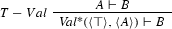
And here is a the validity-version of S4:
It cannot occur in the three places, because then there will be some finite stage n where the formula appears for the first time in the branch in the three sides. But then that sequent will be an axiom, and therefore the branch will be closed.


References
Avron, A. (2007). Non-deterministic semantics for logics with a consistency operator. Journal of Approximate Reasoning, 45, 271–287.
Avron, A., & Zamansky, A. (2008). Non-deterministic semantics for logical systems. In D. Gabbay & F. Guenthner (Eds.), Handbook of philosophical logic (pp. 227–304). Berlin: Springer.
Barrio, E., Rosenblatt, L., Tajer, D. (2016). Capturing naive validity in the cut-free approach. Synthese https://doi.org/10.1007/s11229-016-1199-5.
Beall, J. (2009). Spandrels of truth. Oxford: Oxford University Press.
Beall, J. (2011). Multiple-conclusion lp and default classicality. The Review of Symbolic Logic, 4(02), 326–336.
Beall, J., & Murzi, J. (2013). Two flavors of curry paradox. Journal of Philosophy, 110, 143–165.
Burguess, J., Boolos, G., & Jeffrey, R. (2007). Computability and logic (5th ed.). Cambridge: Cambridge University Press.
Coniglio, M. E., & Da Cruz, L. H. (2014). An alternative approach for quasi-truth. Logic Journal of IGPL, 22(2), 387–410.
Goodship, L. (1996). On dialethism. Australasian Journal of Philosophy, 74(1), 153–161.
Meadows, T. (2014). Fixed points for consequence relations. Logique et Analyse, 57(227), 333–357.
Negri, S. (2005). Proof analysis in modal logic. Journal of Philosophical Logic, 34, 507–544.
Pailos, F., & Tajer, D. (2017). Validity in a dialetheist framework. Logique et Analyse, 70(238), 191–202.
Paoli, F. (2002). Substructural Logics: A Primer. Trends in Logic, Vol 13. Springer, Science Business Media, Dordrecht.
Priest, G. (1979). The Logic of Paradox. Journal of Philosophical Logic, 8(1), 219–241.
Priest, G. (2006). Contradiction: A study of the transconsistent. Oxford: Oxford University Press.
Ripley, D. (2012). Conservatively extending classical logic with transparent truth. Review of Symbolic Logic, 5(2), 354–378.
Sette, A. (1973). On the propositional calculus p1. Mathematica Japonicae, 16, 173–180.
Yablo, S. (1993). Paradox without self-reference. Analysis, 53(4), 251–252.
Acknowledgements
This work was supported by The National Scientific and Technical Research Council (CONICET), and has benefited greatly from discussions with Graham Priest, David Ripley, Eduardo Barrio, Natalia Buacar, Lucas Rosenblatt, Damian Szmuc, Diego Tajer and Paula Teijeiro.
Author information
Authors and Affiliations
Corresponding author
Additional information
This work was supported by The National Scientific and Technical Research Council (CONICET), and has benefited greatly from discussions with Graham Priest, David Ripley, Eduardo Barrio, Natalia Buacar, Lucas Rosenblatt, Damian Szmuc, Diego Tajer and Paula Teijeiro.
Rights and permissions
About this article

Cite this article
Pailos, F.M. Validity, dialetheism and self-reference. Synthese 197, 773–792 (2020). https://doi.org/10.1007/s11229-018-1731-x
Received:
Accepted:
Published:
Issue Date:
DOI: https://doi.org/10.1007/s11229-018-1731-x