OGY-based control of chaos in semi-passive dynamic walking of a torso-driven biped robot

Abstract

This paper aims at controlling chaos exhibited in the semi-passive dynamic walking of a torso-driven biped robot as it goes down an inclined surface. Our control approach is based on the OGY method. The proposed biped robot is a three-degrees-of-freedom planar biped having an impulsive hybrid nonlinear dynamics. For this walker, we use only one torque between the stance leg and the torso in order to control the torso at some desired position and then in order to generate a semi-passive gait. The desired torso angle is considered as the control parameter in our OGY-based control approach. We develop a reduced simple impulsive hybrid linear model by linearizing the impulsive hybrid nonlinear dynamics around a desired period-1 hybrid limit cycle. This conducts to determine an explicit expression of a constrained controlled Poincaré map. A linearization of the controlled Poincaré map around its fixed point permits to looking for the gain matrix of the stabilizing control law. We show that application of the developed OGY-based control parameter law has controlled the chaotic semi-passive gait.

1 Introduction

In research on bipedal walking robots, passive dynamic walking has shown to be a promising approach in applications where energy efficiency of walking is very important. The passive dynamic walking is a walking method for which the biped robot does not require any exogenous source of energy [1–10]. However, it uses only the effect of gravity to move down an inclined surface. The most famous biped model that uses this walking mode is the compass-like biped robot [2–4]. Furthermore, the passive dynamic walking approach has been served as a starting point for designing mechanisms that require little energy, and also for designing some controllers that improve stability and robustness of the locomotion of biped robots [9, 11]. Furthermore, several approaches (such as [10, 12, 13]) explicitly use the knowledge obtained in passive dynamic walking for control. Actuated dynamic walking as opposite to the passive dynamic walking is meant to make the mechanism controllable while the mechanism itself is constructed, so that the effects making the passive dynamic walking possible would as much as possible contribute to an energy efficient bipedal locomotion. From this point, the semi-passive dynamic walking of biped robots is also an approach that contributes to an energy efficiency. In this walking method, the biped robot uses some actuators at its joints as it goes down a sloped ground. Recently, we used this walking type for a torso-driven biped robot: a compass-gait biped robot for which we added a torso as an upper body [14–16]. We used a unique torque between the torso and the stance leg in order to control the torso at some desired position. Thus, the swing leg was completely passive.

Mathematical walking models of biped robots have been known that are described by an impulsive hybrid nonlinear dynamics [17]. Because of such impulsive hybrid feature, the gait model of biped robots can display very interesting and attractive behaviors, namely chaos and bifurcations. It is known so far that passive dynamic walking of biped robots displays chaos and period-doubling bifurcations [18, 19]. Iqbal et al. [7] provide an overview of previous literature on the chaotic behavior of passive dynamic biped robots. We showed recently that the passive dynamic walking of a compass-gait model and the semi-passive dynamic walking of a torso-driven biped model exhibit, besides chaos and period-doubling bifurcations, additional and complex nonlinear phenomena such as cyclic-fold bifurcations, intermittency, interior and boundary crisis [14–16, 20, 21]. Thus, the control of these undesired phenomena will be tremendously needed.

Since the publication of the seminal paper of the pioneering work of Ott et al. [22], controlling chaos has become more interesting in research and practical applications. Basic methods of controlling chaos may be found in [23–27]. One of these methods is the Ott et al. (OGY) method. In the seminal paper [22], two key ideas were introduced for the OGY method: (i) to use the discrete system model based on linearization of the controlled Poincaré map for controller design, and (ii) to use the recurrence property of chaotic motions and apply control action only at an instant when the motion returns to the neighborhood of a desired state of the orbit. In fact, two crucial features of a chaotic system make it a candidate for OGY control approach. First, this method relies on the presence within the chaotic attractor of an infinite number of unstable periodic orbits. Secondly, the OGY method requires an accessible system control parameter through which an applied control input changes the location of the unstable fixed point (or systematically the unstable limit cycle for a continuous dynamics) and hence its stabilization. Then, by making small time-dependent perturbations to the control parameter of the system, it is possible to stabilize one of the unstable periodic orbits. Efficiency of this method has been confirmed by numerous simulations as well as physical experiments.

In literature, we believe that few works have focused on chaos control for walking dynamics of biped robots [7, 28–33]. Suzuki and Furuta [28] used the OGY method for the stabilization of the passive dynamic walking of a compass-gait biped robot. They used the least square method for the determination of a linear discrete model of the Poincaré map. They chose the torque at the hip of the compass-gait biped as the adjustable control parameter. Recently, in [34], we used the OGY-based control approach in order to control chaos exhibited in the passive dynamic walking of the compass-gait biped robot. We used the hip torque as the controller input in the OGY control law. We resorted to a linearization of the impulsive hybrid nonlinear dynamics of the compass-gait model around a desired limit cycle in order to develop an analytical expression of the controlled Poincaré map.

The first step in designing the OGY control is the development of the controlled Poincaré map. However, the impulsive hybrid nonlinear dynamics of the semi-passive dynamic walking of the torso-driven biped robot complicates this task. Therefore, in order to solve this problem, our intuition is to transform the nonlinear model into a linear one. Nevertheless, validity of the linear model may become questionable if the system trajectory involves states that are too far away from the operating point. Thus, in order to have a linear model fairly close to the nonlinear one, our main objective is to linearize, for a desired set of parameters, the nonlinear model around a desired period-1 hybrid limit cycle within a chaotic attractor. In this paper, the linearization method was adopted by us in [34]. We will show that this strategy gives us a reduced simple impulsive hybrid linear model that will be found to generate almost the same characteristics of the impulsive hybrid nonlinear dynamics. Hence, using the developed linear model, we will determine an explicit expression of a constrained controlled Poincaré map. Its fixed point will be then numerically identified. The desired torso angle of the biped robot will be used as the control parameter in the Poincaré map. In addition, we will linearize the constrained controlled Poincaré map. Besides, we will build the gain matrix of the OGY control that stabilize the linearized Poincaré map and hence that stabilize the fixed point of the constrained Poincaré map. We will show finally that implementation of the developed OGY-based parameter (desired torso angle) control will stabilize the semi-passive gait of the torso-driven biped robot and then will control chaos.

In fact, in [34], as noted before, we have controlled the passive dynamic walking of the compass-gait biped robot. This subject is achieved by introducing a controller (a torque input) at the hip of the biped robot. Hence, the utility of the passive dynamic walking is found to be lost because the compass-gait biped robot is found to be under a control input. Then, an external energy was needed for the compass robot. However, the torso-driven biped robot is the compass-gait biped robot with an upper body (a torso). Moreover, we used a PD controller in order to stabilize the torso at some desired position [14–16]. Thus, we obtained a semi-passive dynamic walking that can be either chaotic or periodic. Then, in order to control the unstable semi-passive gait, we will not employ an additional control input. However, we will use the desired torso angle as the available control parameter, and hence, we will use the torso as a mechanical mechanism to control the semi-passive chaotic gait. As a result, we will not need to a supplementary external energy to control the bipedal locomotion. Accordingly, our main contribution in this work is the control of semi-passive bipedal locomotion without an additional control input and with a maximum energy efficiency, which is an important criterion in bipedal robots [17].

The layout of the rest of the paper is as follows. In Sect. 2, we present the concept of the OGY control method. In Sect. 3, we provide the impulsive hybrid nonlinear dynamics of the semi-passive dynamic walking of the torso-driven biped robot. The semi-passive controller for the biped robot and the problem formulation are given also in this section. Section 4 describes our method adopted for the linearization of the impulsive hybrid nonlinear dynamics around a desired hybrid limit cycle and the development of an impulsive hybrid linear model. In Sect. 5, we determine the analytical expression of a constrained controlled Poincaré map. The linearization of the constrained controlled Poincaré map around the fixed point of the Poincaré map and its stabilization are presented in Sect. 6. The subject of chaos control using the impulsive hybrid nonlinear dynamics is addressed in Sect. 7. Finally, in Sect. 8, some conclusions and future works are presented.

2 Concept of the OGY-based control

The OGY method is based mainly on the linearization of the Poincaré Map. The essential of the OGY-based control method is as follows [24].

Let consider a controlled (nonlinear) system with the following differential equation:

$$\begin{aligned} \dot{\varvec{x}} = \varvec{f}\left( \varvec{x}, u\right) \end{aligned}$$

(1)

where $\varvec{x}\in \mathfrak {R}^{n}$ and $u\in \mathfrak {R}$. We stress that the variable $u$ can be either the changeable system parameter or the standard input control.

We consider the desired trajectory $\varvec{x}_{*}\left( t\right)$ solution of (1) for $u=u_{*}$. For the system (1), we construct the so-called Poincaré section ${\mathcal P_{S}}$:

$$\begin{aligned} {\mathcal P_{S}}=\left\{ \varvec{x}\in \mathfrak {R}^{n}\,:\,s (\varvec{x})=0, \quad s_{\varvec{x}}\varvec{f}(\varvec{x},u_{*}) \ne 0\right\} \end{aligned}$$

(2)

with $s_{\varvec{x}} = \frac{\partial s\left( \varvec{x}\right) }{\partial \varvec{x}}$.

Next, we consider the map $\varvec{x}\longmapsto \varvec{\mathcal P}\left( \varvec{x}, u\right)$ with $\varvec{\mathcal P}\left( \varvec{x}, u\right)$ is the point of the first return to the Poincaré section ${\mathcal P_{S}}$ of the solution of the system (1) with constant input $u$ that begins from the point $\varvec{x}$. The map $\varvec{x}\longmapsto \varvec{\mathcal P}\left( \varvec{x}, u\right)$ is called the controllable Poincaré map.

Iteration of this map conducts to the following discrete system:

$$\begin{aligned} \varvec{x}_{k+1} = \varvec{\mathcal P}(\varvec{x}_{k}, u_{k}) \end{aligned}$$

(3)

where $\varvec{x}_{k} = \varvec{x} (t_{k}), t_{k}$ is the time instant of the $k$th intersection with the Poincaré section ${\mathcal P_{S}}$, and $u_{k}$ is the value of control $u(t)$ over the interval between $t_{k}$ and $t_{k+1}$.

Thus, the first step in designing the OGY control law lies in the determination of the expression of this controlled Poincaré map (3). The second step consists in the identification of the fixed point $\varvec{x}_{*}$ of the Poincaré map for $u=u_{*}$ solution of the following function:

$$\begin{aligned} \varvec{\mathcal P}\left( \varvec{x}_{*}, u_{*}\right) - \varvec{x}_{*} = \varvec{0} \end{aligned}$$

(4)

The next step lies in the linearization of the controlled Poincaré map in order to replace the original system (1) by the following linearized discrete system:

$$\begin{aligned} \varvec{\delta x}_{k+1} = \varvec{\mathcal A}\,\varvec{\delta x}_{k} + \varvec{\mathcal B}\,\delta u_{k} \end{aligned}$$

(5)

where $\varvec{\delta x}_{k} = \varvec{x}_{k} - \varvec{x}_{*}, \delta u_{k} = u_{k} - u_{*}$, and

$$\begin{aligned} \varvec{\mathcal A} = \frac{\partial }{\partial \varvec{x_{k}}}\varvec{\mathcal P}\left( \varvec{x}_{*}, u_{*}\right) ,\quad \varvec{\mathcal B} = \frac{\partial }{\partial \varvec{u_{k}}}\varvec{\mathcal P} (\varvec{x}_{*}, u_{*}). \end{aligned}$$

The forth step in designing the OGY controller lies in the search for the gain $\varvec{\mathcal K}$ of the stabilizing control law:

$$\begin{aligned} \delta u_{k}=\varvec{\mathcal K}\,\varvec{\delta x}_{k} \end{aligned}$$

(6)

for the linear discrete system (5).

Finally, we apply the OGY-based controller

$$\begin{aligned} u_{k} = u_{*} + \varvec{\mathcal K}\,\left( \varvec{x}_{k}-\varvec{x}_{*}\right) \end{aligned}$$

(7)

to the initial system (1).

It is noteworthy that the main key in designing the OGY control for the (nonlinear) system (1) is the determination of an explicit expression of the controlled Poincaré map (3). In this work, we will use this OGY method to control chaos exhibited in the impulsive hybrid nonlinear dynamics of the semi-passive dynamic walking of the torso-driven biped robot.

3 Semi-passive dynamic walking of the torso-driven biped robot

This section gives the walking dynamics of the semi-passive torso-driven biped robot as it goes down an inclined plane and its walking patterns as some bifurcation parameter varies.

3.1 The semi-passive torso-driven biped robot model

A schematic representation of the torso-driven biped robot is provided in Fig. 1 [14–16]. The significant parameters in the dynamics description are given in Table 1. This planar biped robot is in fact a compass-gait biped model [21, 34] for which we added a torso as an upper body. This biped robot is a subclass of rigid mechanical systems subject to unilateral constraints. It has only three degrees of freedom. The torso-driven biped robot is composed of two identical legs: a swing leg and a stance leg, a frictionless hip and a torso. Each leg has a lumped mass $m$ concentrated at a distance $b$ from the hip that has a mass $m_{H}$. The torso has a point mass $m_{T}$ located at a distance $r$ from the hip joint. The torso is employed to drive the biped robot on the walking surface of slope $\varphi$. The configuration of the biped walker is essentially determined by the stance angle $\theta _{s}$, the nonsupporting (swing) angle $\theta _{ns}$ and the torso angle $\theta _{t}$. Positive angles are calculated in the counterclockwise direction relative to the indicated vertical lines.

Fig. 1

Schematic of the semi-passive torso-driven biped robot on a slope $\varphi$

Table 1 Specification of simulation parameters for the torso-driven biped robot model

It is well known that the passive compass-gait biped robot is powered only by gravity without any actuation, and with an adequate initial configuration, it walks passively and indefinitely down an inclined surface. Then, in order to have the passive form of the bipedal walk for he torso-driven biped robot, we have used only a control law $u$ between the torso and the stance leg. The main role of this control law is to stabilize the torso at some desired position, while the swing leg is maintained unactuated and its motion is completely passive. Accordingly, depending on the initial configuration, the dynamic walking of the torso-driven biped robot is defined as semi-passive.

3.2 Impulsive hybrid nonlinear dynamics

The model of the semi-passive dynamic walking of the torso-driven biped robot consists of a continuous dynamics of the swing phase and algebraic equations of the impulsive impact phase. The continuous dynamics and the algebraic equations form a complex system defined as an impulsive hybrid nonlinear dynamics.

3.2.1 Modeling hypotheses

For the design of the semi-passive dynamic walking of the torso-driven biped robot, we have considered some assumptions:

• The biped robot is planar, whose movement is constrained in the sagittal plane,

• The biped robot consists of straight rigid segments, and it is without knees and feet,

• The dynamic walking of the biped robot consists of two alternating phases: a swing phase and a very instantaneous impact phase,

• The stance leg acts as a pivot during the swing phase,

• The swing leg undergoes neither slipping nor rebound at the impact,

• The bipedal locomotion is from left to right, so that the swing leg moves behind the stance leg and touches the ground at the impact phase in front of the stance leg.

• After impact, the stance leg leaves the ground without any interaction with the walking surface,

• The reaction force due to the impact can be modeled as an impulse. The impulsive force has as a result discontinuous changes in the angular velocities of the biped robot, while the position states remain continuous.

• The contact of the swing leg with the inclined surface is modeled as a contact between two rigid bodies.

Furthermore, we stress that when the two legs are overlapped during the swing stage, the scuffing problem of the swing leg with the ground is neglected in simulation.

3.2.2 Continuous dynamics of the swing phase

The continuous dynamics of the torso-driven biped robot as it goes down an inclined plane translates the bipedal motion during the swing phase. It describes the situation when the stance leg is fixed on the ground as a pivot and the swing leg swings forward while walking down the slope. Then, the continuous dynamics will be represented by a set of nonlinear differential equations.

Let $\varvec{\theta }=\left[ \begin{array}{ccc} \theta _{ns}&\,\theta _{s}&\,\theta _{t} \end{array} \right] ^\mathrm{T}$ be the vector of generalized coordinates of the torso-driven biped robot. Then, under certain assumptions noted before, the swing motion can be described by the following Euler–Lagrange system:

$$\begin{aligned} \varvec{{\mathcal J}}(\varvec{\theta })\varvec{\ddot{\theta }}+\varvec{{\mathcal H}}(\varvec{\theta },\varvec{\dot{\theta }})+\varvec{{\mathcal G}}(\varvec{\theta })=\varvec{{\mathcal B}}u \quad \text {as long as}\quad \varvec{\theta }\in \varOmega , \end{aligned}$$

(8)

where $\mathcal J$ is the inertia matrix, $\mathcal H$ includes Coriolis and centrifugal terms, $\mathcal G$ includes gravity forces, and $\mathcal B$ is the input matrix. These matrices are defined like so:

$$\begin{aligned}&{\varvec{\mathcal J}}(\varvec{\theta }) = \left[ \begin{array}{ccc} mb^2 &{} \quad -mlb \cos (\theta _{s}-\theta _{ns}) &{}\quad 0\\ -mlb \cos (\theta _{s}-\theta _{ns}) &{}\quad ma^2+(m+m_{H}+m_{T})l^2 &{}\quad m_{T}rl \cos (\theta _{s}-\theta _{t})\\ 0 &{}\quad m_{T}rl \cos (\theta _{s}-\theta _{t}) &{}\quad m_{T}r^2 \end{array}\right] ,\\&{\varvec{\mathcal H}}(\varvec{\theta },\dot{\varvec{\theta }})= \left[ \begin{array}{c} mlb\dot{\theta }_{s}^2 \sin (\theta _{s}-\theta _{ns})\\ -mlb\dot{\theta }_{ns}^2 \sin (\theta _{s}-\theta _{ns}) +m_{T}rl\dot{\theta }_{t}^2 \sin (\theta _{s}-\theta _{t})\\ -m_{T}rl\dot{\theta }_{s}^2 \sin (\theta _{s}-\theta _{t}) \end{array}\right] ,\\&{\varvec{\mathcal G}}(\varvec{\theta }) = g\left[ \begin{array}{c} mb \sin (\theta _{ns})\\ -(ma+(m+m_{H}+m_{T})l)\sin (\theta _{s})\\ -m_{T}r\sin (\theta _{t}) \end{array} \right] ,\quad \hbox {and}\quad {\varvec{\mathcal B}} = \left[ \begin{array}{c} 0\\ 1\\ -1 \end{array}\right] . \end{aligned}$$

While going down the inclined plane, the torso-driven biped robot is in fact subject to only one natural unilateral constraint defined by expression (9). This expression corresponds to the distance between the tip of the swing leg and the ground. It represents the situation that the swing leg is always above the ground.

$$\begin{aligned} \varOmega&= \left\{ \varvec{\theta }\in \mathfrak {R}^{3}\,:\,{\mathcal L}_{1}(\varvec{\theta })=l\left( \cos (\theta _{s}+\varphi )\right. \right. \nonumber \\&\left. \left. -\cos (\theta _{ns}+\varphi )\right) >0\right\} . \end{aligned}$$

(9)

In fact, depending on the initial conditions, the geometric and inertial properties of the biped robot and the inclination of the ground $\varphi$, a contact of the swing leg with the walking surface can occur just at the beginning of the swing phase and when the two legs are overlapped (scuffing problem). Then, in our numerical simulations, these two situations are neglected during the swing phase. In fact, in order to avoid the scuffing problem for a real biped robot, we can use a prismatic joint at each leg as in [2, 10]. Thus, we will assume that the natural unilateral constraint (9) will be satisfied during the swing phase.

3.2.3 Algebraic equations of the impact phase

The instantaneous contact of the swing leg with the walking surface induces impulsive transitions in the vector of angular velocities $\varvec{\dot{\theta }}$ of the torso-driven biped robot. These impulsive effects are translated by some defined algebraic equations. At the impact, a switching of the swing leg and the stance one occurs: that is, the swing leg becomes the stance one and vice versa. The impact phase occurs when the three following conditions are well satisfied:

• 1. the swing leg reaches the ground,

• 2. the swing leg is moving downward,

• 3. the swing leg is in front of the stance leg.

In fact, the third condition is added in order to avoid the scuffing problem. These three impact constraints can be translated by the following set which describes the expression of the impact surface $\varGamma$:

$$\begin{aligned} \varGamma {=}\left\{ \begin{array}{l} {\mathcal L}_{1}(\varvec{\theta }) =l\left( \cos (\theta _{s}+\varphi )-\cos (\theta _{ns}+\varphi )\right) =0\\ {\mathcal L}_{2}(\varvec{\theta },\varvec{\dot{\theta }}) =l\left( \sin (\theta _{ns}+\varphi )\dot{\theta }_{ns}\right. \\ \left. \qquad \qquad \qquad -\sin (\theta _{s} +\varphi )\dot{\theta }_{s}\right) <0\\ {\mathcal L}_{3}(\varvec{\theta }) = l\left( \sin (\theta _{ns})-\sin (\theta _{s})\right) >0 \end{array}\right\} .\nonumber \\ \end{aligned}$$

(10)

We note that: ${\mathcal L}_{2}(\varvec{\theta },\dot{\varvec{\theta }}) = \frac{\mathrm{d}{\mathcal L}_{1}\left( \varvec{\theta }\right) }{\mathrm{d}t} = \frac{\partial {\mathcal L}_{1}\left( \varvec{\theta }\right) }{\partial \varvec{\theta }} \dot{\varvec{\theta }}$.

Algebraic equations modeling positions and velocities transitions at the impact with the walking surface are expressed by [14, 16]:

$$\begin{aligned} \left\{ \begin{array}{l} \varvec{\theta }^{+} = \varvec{{\mathcal R}}_{e}\varvec{\theta }^{-}\\ \dot{\varvec{\theta }}^{+} = \varvec{{\mathcal S}}_{e}\dot{\varvec{\theta }}^{-} \end{array}\right. \end{aligned}$$

(11)

where subscribes ${+}$ and ${-}$ denote just after and just before the impact phase, respectively. The impulsive impact (11) is described by the renaming matrix $\varvec{{\mathcal R}_{e}}$ and the reset matrix $\varvec{{\mathcal S}_{e}}$. These two matrices are defined by:

$$\begin{aligned}&{\varvec{\mathcal R}}_{e} = \left[ \begin{array}{ccc} 0 &{}\quad 1 &{}\quad 0\\ 1 &{}\quad 0 &{}\quad 0\\ 0 &{}\quad 0 &{}\quad 1 \end{array} \right] ,\\&\varvec{{\mathcal S}}_{e} = \varvec{{\mathcal R}}_{e} - \varvec{{\mathcal R}}_{e}\varvec{{\mathcal M}}_{e}^{-1}\varvec{{\mathcal N}}_{e}\left( \varvec{{\mathcal D}}_{e}^{-1} + \varvec{{\mathcal N}}_{e}^{T}\varvec{{\mathcal M}}_{e}^{-1}\varvec{{\mathcal N}}_{e}\right) ^{-1}\varvec{{\mathcal Q}}_{e},\\&\hbox { where }\\&\varvec{{\mathcal M}}_{e} = \varvec{{\mathcal J}}-\varvec{{\mathcal C}}_{e}\varvec{{\mathcal D}}_{e}^{-1}\varvec{{\mathcal C}}_{e}^{T},\quad \varvec{{\mathcal N}}_{e} = \varvec{\mathcal Q}_{e}^{T} - \varvec{{\mathcal C}}_{e}\varvec{{\mathcal D}}_{e}^{-1},\quad {\varvec{\mathcal D}}_{e}=\left( 2m+m_{H}+m_{T}\right) \varvec{\mathcal I}_{2},\\&{\varvec{\mathcal C}}_{e} = \left[ \begin{array}{cc} mb \cos (\theta _{ns}) &{}\quad mb\sin (\theta _{ns})\\ -\left( ma+\left( m+m_{H}+m_{T}\right) l\right) \cos (\theta _{s}) &{}\quad -\left( ma+\left( m+m_{H}+m_{T}\right) l\right) \sin (\theta _{s})\\ -m_{T}r\cos (\theta _{t}) &{}\quad -m_{T}r\sin (\theta _{t}) \end{array}\right] ,\\&{\varvec{\mathcal Q}}_{e}=\left[ \begin{array}{ccc} l\cos (\theta _{ns}) &{}\quad -l\cos (\theta _{s})&{} \quad 0\\ l\sin (\theta _{ns}) &{}\quad -l\sin (\theta _{s}) &{}\quad 0 \end{array} \right] , \,\hbox {and}\,\, {\varvec{\mathcal I}_{2}}\,\, \hbox {is\, the\, identity\, matrix\, of\, dimension\, 2.} \end{aligned}$$

3.2.4 Semi-passive control law

Our main goal was to achieve an efficient semi-passive dynamic walking of the torso-driven biped robot while walking down an inclined surface by controlling the torso at some desired position (desired torso angle $\theta ^{d}_{t}$). We then apply an output feedback control for the torso, so that it will be stabilized at the desired position. Thus, $\theta _{t}$ is the control output. The second-order derivative with respect to time becomes:

$$\begin{aligned} \ddot{\theta }_{t} = \varvec{\mathcal C}\varvec{\mathcal M}(\varvec{\theta },\dot{\varvec{\theta }}) + \varvec{\mathcal C}\varvec{\mathcal N}(\varvec{\theta })u, \end{aligned}$$

(12)

where $\varvec{\mathcal C}{=}\left[ \begin{array}{ccc} 0&\,\, 0&\,\, 1 \end{array}\right] , \varvec{{\mathcal M}}(\varvec{\theta },\dot{\varvec{\theta }}){=}-\varvec{{\mathcal J}}(\varvec{\theta })^{-1}\big (\varvec{{\mathcal H}}(\varvec{\theta },\dot{\varvec{\theta }})$ $+\varvec{{\mathcal G}}(\varvec{\theta })\big )$, and $\varvec{{\mathcal N}}(\varvec{\theta })=\varvec{{\mathcal J}}(\varvec{\theta })^{-1}\varvec{{\mathcal B}}$.

The control input, $u$, for achieving $\theta _{t}\longrightarrow \theta ^{d}_{t}$ can be determined as

$$\begin{aligned} \left\{ \begin{array}{l} u = \left( \varvec{\mathcal C}\varvec{{\mathcal N}}(\varvec{\theta })\right) ^{-1}\left( v-\varvec{\mathcal C}\varvec{\mathcal M}(\varvec{\theta },\dot{\varvec{\theta }})\right) \\ v = -{\mathcal K}_{d}\dot{\theta }_{t}+{\mathcal K}_{p}(\theta ^{d}_{t}-\theta _{t}) \end{array}\right. \end{aligned}$$

(13)

where ${\mathcal K}_{p}$ and ${\mathcal K}_{d}$ are two scalar gains of the control law $u$.

Hence, expression of $u$ in (13) describes the semi-passive control law that will be applied to the torso-driven biped robot as it goes down the inclined surface in order to control the torso at the desired position $\theta ^{d}_{t}$ and accordingly to obtain a semi-passive dynamic walking.

3.2.5 Complete model of the semi-passive dynamic walking

Expressions (8)–(11) and (13) form the nonlinear impulsive hybrid dynamics of the semi-passive dynamic walking of the torso-driven biped robot. The differential equation in (8) can be rewritten like so:

$$\begin{aligned} \varvec{\ddot{\theta }} = \varvec{\mathcal M}(\varvec{\theta },\dot{\varvec{\theta }}) + \varvec{\mathcal N}(\varvec{\theta })u. \end{aligned}$$

(14)

Furthermore, expression of $v$ in (13) can be rewritten as $v = -\varvec{\mathcal C}\left( {\mathcal K}_{p}\varvec{\theta } + {\mathcal K}_{d}\dot{\varvec{\theta }}\right) + {\mathcal K}_{p}\theta ^{d}_{t}$. Then, substituting (13) into (14) yields:

$$\begin{aligned} \varvec{\ddot{\theta }} \!&= \! \left( \varvec{\mathcal I}_{3}{-}\frac{\varvec{\mathcal N}(\varvec{\theta })\varvec{\mathcal C}}{\varvec{\mathcal C}\varvec{\mathcal N}(\varvec{\theta })}\right) \varvec{\mathcal M}(\varvec{\theta },\dot{\varvec{\theta }}) {-} \frac{\varvec{\mathcal N} \varvec{\theta })\varvec{\mathcal C}}{\varvec{\mathcal C}\varvec{\mathcal N}(\varvec{\theta })}\left( {\mathcal K}_{p}\varvec{\theta } + {\mathcal K}_{d}\dot{\varvec{\theta }}\right) \nonumber \\&\quad +\,\frac{\varvec{\mathcal N}(\varvec{\theta })}{\varvec{\mathcal C}\varvec{\mathcal N}(\varvec{\theta })}{\mathcal K}_{p}\theta ^{d}_{t}, \end{aligned}$$

(15)

where $\varvec{\mathcal I}_{3}$ is the identity matrix of dimension 3.

Let $\varvec{x}=\left[ \begin{array}{cc} \varvec{\theta }^{T}&\,\dot{\varvec{\theta }}^{T} \end{array} \right] ^\mathrm{T}$ be the state vector. Thus, the semi-passive impulsive hybrid nonlinear dynamics defined by (15), (9)–(11) is reformulated as follows:

$$\begin{aligned} \left\{ \begin{array}{ll} \dot{\varvec{x}} = \varvec{\mathcal F}(\varvec{x},\theta ^{d}_{t}) = \varvec{f}(\varvec{x})+\varvec{g} (\varvec{x})\theta ^{d}_{t}&{}\quad \text {as long as} \quad \varvec{x}\in \varOmega \\ \varvec{x}^{+} ={\varvec{h}}\left( \varvec{x}^{-}\right) &{} \quad \text {whenever} \quad \varvec{x}^{-}\in \varGamma \end{array}\right. \end{aligned}$$

(16)

where

$$\begin{aligned} \left\{ \begin{array}{l} \varOmega = \left\{ \varvec{x}\in \mathfrak {R}^{6}\,:\,{\mathcal L}_{1}\left( \varvec{x}\right) >0\right\} \\ \varGamma = \left\{ \varvec{x}\in \mathfrak {R}^{6}: {\mathcal L}_{1}\left( \varvec{x}\right) = 0, \;\; {\mathcal L}_{2}\left( \varvec{x}\right) < 0, \;\; {\mathcal L}_{3}\left( \varvec{x}\right) > 0 \right\} \end{array}\right. \end{aligned}$$

(17)

and $\varvec{x}^{+}$ denotes the value of $\varvec{x}$ just after the impact, and $\varvec{x}^{-}$ denotes the value of $\varvec{x}$ just before the impact.

In (16), $\varvec{f}(\varvec{x})=\left[ \begin{array}{c} \dot{\varvec{\theta }} \\ \left( \varvec{\mathcal I}_{3}-\frac{\varvec{\mathcal N}(\varvec{\theta })\varvec{\mathcal C}}{\varvec{\mathcal C}\varvec{\mathcal N}(\varvec{\theta })}\right) \varvec{\mathcal M}(\varvec{\theta },\dot{\varvec{\theta }})\\ - \frac{\varvec{\mathcal N}(\varvec{\theta })\varvec{\mathcal C}}{\varvec{\mathcal C}\varvec{\mathcal N}(\varvec{\theta })} \left( {\mathcal K}_{p}\varvec{\theta } + {\mathcal K}_{d}\dot{\varvec{\theta }}\right) \end{array} \right] \hbox {and} \varvec{g}(\varvec{x})\!=\!\left[ \begin{array}{c} \varvec{0}_{3 \times 1}\\ \frac{\varvec{\mathcal N}(\varvec{\theta })}{\varvec{\mathcal C}\varvec{\mathcal N}(\varvec{\theta })} {\mathcal K}_{p}\\ \end{array} \right] \!, \hbox { and } {\varvec{h}}\left( \varvec{x}\right) \!=\! \left[ \begin{array}{cc} \varvec{{\mathcal R}}_{e} &{}\quad \varvec{{0}}_{3\times 3}\\ \varvec{{0}}_{3\times 3} &{}\quad \varvec{{\mathcal S}}_{e} \end{array}\right] \varvec{x}.$

Fig. 2

Bifurcation diagrams: variation of the step period as a function of the slope angle $\varphi$ (a) and as a function of the desired torso angle $\theta ^{d}_{t}$ (b)

The solution of the impulsive hybrid nonlinear dynamics defined by (16) and (17) of the torso-driven biped robot can be expressed in terms of flow as:

$$\begin{aligned} \varvec{x}(t)=\varvec{\phi }\left( t,\varvec{x}_{0}\right) , \end{aligned}$$

(18)

where $\varvec{x}_{0}=\varvec{\phi }\left( t_{0},\varvec{x}_{0}\right)$ is the initial condition of the semi-passive gait.

In fact, the nonlinear dynamics (16) is expressed in function of the desired torso angle $\theta ^{d}_{t}$ because it will be used next as the adjustable control parameter for the OGY-like method in order to control chaos in the semi-passive dynamic walking of the torso-driven biped robot.

3.3 Semi-passive walking dynamics of the torso-driven biped robot

We showed in [14–16] that the semi-passive dynamic walking of the torso-driven biped robot exhibits different nonlinear phenomena such as bifurcations and chaos as some bifurcation parameter varies. Figure 2 reveals the semi-passive walking patterns for two bifurcation parameters, namely the slope angle $\varphi$ (Fig. 2a) and the desired torso angle $\theta ^{d}_{t}$ (Fig. 2b). The first bifurcation diagram was plotted for $\theta ^{d}_{t}=0^{\circ }$, whereas the second one (Fig. 2b) was plotted for $\varphi =5^{\circ }$. These two bifurcation diagrams show two distinct attractors: $A_{1}$ depicted in blue and $A_{2}$ plotted in red. The former reveals the scenario of period-doubling route to chaos. The first period-doubling bifurcation is indicated as PDB. This PDB creates a period-1 unstable periodic orbit or a period-1 unstable limit cycle (dashed green line indicated by p1-UPO). However, the latter attractor $A_{2}$ shows the new walking dynamics revealing a scenario of a period-three route to chaos generated by means of a cyclic-fold bifurcation (marked by CFB) [16, 21]. At this bifurcation, two period-3 periodic orbits, one stable and another unstable (dashed pink line indicated by p3-UPO), meet and annihilate with each other.

We emphasize that stability of a limit cycle (or a periodic orbit) of the semi-passive gait is investigated by means of the Poincaré map’s concept. Thus, the analysis of the limit cycle is reduced to the study of its fixed point (i.e., the fixed point of the Poincaré map). Furthermore, stability of the fixed point is investigated by analyzing the eigenvalues of the Jacobian matrix of the Poincaré map or systematically the monodromy matrix [35, 36]. In [16], we have employed this methodology to study the stability of the hybrid limit cycle of the impulsive hybrid nonlinear dynamics of biped robots.

Furthermore, we emphasize that, in order to detect the period-one unstable periodic orbits (p1-UPO) and the other periodic ones, we used the shooting method and the iterative Newton–Raphson scheme [35]. In [16, 21], we used the shooting method and the iterative Davidchak–Lai method in order to detect the p3-UPO (the dashed pink line) for the compass-gait model. The difference between these two methods is indicated in [21]. Then, firstly, we need to detect one unstable fixed point of the limit cycle (UPO) for some specified bifurcation parameter. Let the first detected unstable fixed point be near the period-doubling (or cyclic-fold) bifurcation. Then, using this old fixed point, we increase slightly and gradually the value of the bifurcation parameter and we look for the new unstable fixed point using the Newton–Raphson method, and so on. Finally, we join the identified unstable fixed points to form the dashed curves.

Figure 3 shows a stable period-1 hybrid limit cycle of the torso-driven biped robot for two defined parameters: $\varphi =3^{\circ }$ and $\theta ^{d}_{t}=0^{\circ }$. In fact, Fig. 3a reveals the limit cycle of the two legs, whereas Fig. 3b shows the limit cycle of the torso. The hybrid limit cycle of the two legs is composed of two parts: the blue part reveals the passive gait of the swing leg, and the pink part presents the semi-passive gait of the stance leg. In fact, the period-1 hybrid limit cycle of the torso-driven biped robot reveals a stable period-1 semi-passive gait. Solid squares indicate the impact point of the swing leg with the walking surface. However, solid circles show the initial conditions of the two legs and the torso just after the impact phase.

We showed in [14] that the torso and then the desired torso angle $\theta ^{d}_{t}$ can be used to control the semi-passive gait of the biped robot.

Fig. 3

Period-1 hybrid limit cycle of the semi-passive dynamic walking of the torso-driven biped robot for a slope angle $\varphi =3^{\circ }$ and a desired torso angle $\theta ^{d}_{t}=0^{\circ }$

3.4 Problem formulation

We emphasize that in the all semi-passive walking dynamics shown in Fig. 2, only the period-1 stable and unstable periodic orbits reveal a symmetric gait of the torso-driven biped robot. The other gaits and in particular the chaotic gaits are asymmetric. In fact, for a symmetric gait, any two consecutive steps are indistinguishable, that is, all gait descriptors and then all spatiotemporal variables exactly repeat themselves in each step. Hence, the main objective in robotics is to control biped robots in order to obtain a stable symmetric gait with remarkably human-like motion. Furthermore, it is absolutely necessary to control biped robots with a maximum energetic efficiency, which is the main motivation behind the design and the use of the passive dynamic walking. Thus, the design of an active dynamic walking of a biped robot should be based on an approach that emphasizes the passive dynamics of the two legs and that particularly avoids the use of high-gain control. In [34], we showed that the use of the OGY-based control method for the compass-gait biped robot to control chaos increases the energy efficiency of the bipedal locomotion and the control gain is very small.

In the present work, we interested in the use of the OGY-based control approach to control chaos exhibited in the semi-passive dynamic walking of the torso-driven biped robot in order to obtain a stable symmetric gait with a maximum energy efficiency. For the biped robot, we will not employ an additional torque to control the semi-passive dynamic walking. But we will use the OGY-based control approach, and we will use the desired torso angle as an accessible changeable control parameter. As mentioned before, the control of a chaotic gait lies on the control of an unstable period-1 limit cycle embedded into the chaotic attractor. Accordingly, the control of chaos based on the OGY approach requires the identification of such unstable period-1 limit cycle and its stabilization by designing a specific controller. However, the stabilization of the unstable limit cycle based on the OGY method requires chiefly the determination of an explicit expression of the controlled Poincaré map. However, the impulsive hybrid nonlinear dynamics, (16) and (17), of the semi-passive dynamic walking of the torso-driven biped robot complicates this task. Then, in order to obtain an analytical expression of the controlled Poincaré map, we will adopt the method used by us in [34] in order to transform the nonlinear model into a linear one. This transformation was achieved by linearizing the nonlinear model around a desired period-1 hybrid limit cycle. As a result, we obtained a reduced impulsive hybrid linear dynamics. The next section describes the method adopted for the linearization.

Fig. 4

Subdivision of the desired flow $\varvec{\phi }_{d}\left( t,\varvec{x}_{0}\right)$ of the semi-passive symmetric gait of the torso-driven biped robot for a desired set of parameters $\lambda _{d} = \left\{ \varphi , \theta ^{d}_{t}\right\}$

4 Determination of the reduced impulsive hybrid linear model

Our main objective was to develop a linear model of the semi-passive dynamic walking of the torso-driven biped robot. This linear model must absolutely generate almost the same gait descriptors of the nonlinear model defined by (16) and (17) for some set of parameters. Then, in order to accomplish our goal, we must resort to a linearization of the nonlinear model around a desired hybrid limit cycle for some desired parameters [34]. We stress that for each set of parameters, there is always a limit cycle that can be either stable or unstable. Thus, and particularly, there exists an unstable period-1 limit cycle for a chaotic semi-passive gait.

4.1 Linearization of the nonlinear model

Let $\lambda _{d} = \left\{ \varphi , \theta ^{d}_{t}\right\}$ be the desired set of parameters of the semi-passive gait. Then, for some defined $\lambda _{d}$, we have a desired period-1 limit cycle $\varLambda _{d}$ (like the period-1 limit cycle in Fig. 3) and hence a desired trajectory (flow) $\varvec{\phi }_{d}\left( t,\varvec{x}_{0}\right)$ for only one walking step. Thus, $\varLambda _{d}$ will be characterized also by the desired step period or the desired impact instant $\tau _{d}$. Then, the desired flow will be defined in the interval $\left[ \begin{array}{cc} 0&\, \tau _{d} \end{array} \right]$. Figure 4 shows the desired flow of the semi-passive gait of the biped robot for $t \in \left[ \begin{array}{cc} 0&\, \tau _{d} \end{array} \right]$.

To build a linear model that generates a flow very close to the flow $\varvec{\phi }\left( t,\varvec{x}_{0}\right)$ of the nonlinear model, we have resorted to a linearization of this nonlinear model around the desired period-1 limit cycle $\varLambda _{d}$ (of the desired flow $\varvec{\phi }_{d}\left( t,\varvec{x}_{0}\right)$). Thus, this linearization lies in the determination of $n$ different elementary linear model $M_{i}$, for $i=1,2,\ldots ,n$, around different points $\varvec{\chi }_{i}$ of the desired flow $\varvec{\phi }_{d}\left( t,\varvec{x}_{0}\right)$. Each linear submodel $M_{i}$ will be valid only for some defined time interval. Then, we will subdivide the desired time interval $\left[ \begin{array}{cc} 0&\, \tau _{d} \end{array} \right]$ into $n$ subintervals $\left[ \begin{array}{cc} t_{\left( i-1\right) }&\, t_{i} \end{array} \right]$, where, for $i=1,2,\ldots ,n$, the instant $t_{i}$ is defined as:

$$\begin{aligned} t_{i}=\frac{i}{n}\tau _{d}. \end{aligned}$$

(19)

We note that $\varvec{x}\left( t_{0}\right) =\varvec{\phi }_{d} \left( t_{0},\varvec{x}_{0}\right)$ and $\varvec{x} \left( t_{n}\right) =\varvec{\phi }_{d}\left( \tau _{d}, \varvec{x}_{0}\right)$. Therefore, each elementary linear model $M_{i}$ will be valid only in $\left[ \begin{array}{cc} t_{\left( i-1\right) }&\, t_{i} \end{array} \right]$. A judicious choice of the point $\varvec{\chi }_{i}$ is to be at the instant in the middle of the subinterval $\left[ \begin{array}{cc} t_{\left( i-1\right) }&\, t_{i} \end{array} \right]$. Thus, the point $\varvec{\chi }_{i}$ will be defined by $\varvec{\chi }_{i}=\varvec{x}\left( \frac{t_{i}+t_{\left( i-1\right) }}{2}\right) =\varvec{x}\left( \frac{2i-1}{2n}\tau _{d}\right)$. Figure 4 shows the subdivision of the desired flow $\varvec{\phi }_{d}\left( t,\varvec{x}_{0}\right)$ of the symmetric semi-passive gait of the torso-driven biped robot.

Let consider the nonlinear differential equation in (16) of the continuous dynamics. An elementary linearized model $M_{i}$ around the point $\varvec{\chi }_{i}$ is defined, for all $i=1,2,\ldots ,n$, by:

$$\begin{aligned} \dot{\varvec{x}}=\varvec{A}_{i}{\varvec{x}} + \varvec{b}_{i}\quad \text {for}\quad t_{\left( i-1\right) } \le t \le t_{i}, \end{aligned}$$

(20)

with $\varvec{A}_{i}=\frac{\partial }{\partial \varvec{x}}\varvec{\mathcal F}(\varvec{\chi }_{i},\theta ^{d}_{t})$, and $\varvec{b}_{i}=\varvec{\mathcal F}\left( \varvec{\chi }_{i},\theta ^{d}_{t}\right) -\varvec{A}_{i}\varvec{\chi }_{i}$.

As $\varvec{\mathcal F}(\varvec{x},\theta ^{d}_{t}) = \varvec{f}(\varvec{x})+\varvec{g}(\varvec{x}) \theta ^{d}_{t}$, it follows that: $\frac{\partial \varvec{\mathcal F}(\varvec{x},\theta ^{d}_{t})}{\partial \varvec{x}}=\frac{\partial \varvec{f}(\varvec{x})}{\partial \varvec{x}} + \frac{\partial \varvec{g}(\varvec{x})}{\partial \varvec{x}}\theta ^{d}_{t} = \varvec{f}_{\varvec{x}}(\varvec{x}) + \varvec{g}_{\varvec{x}}(\varvec{x})\theta ^{d}_{t}$, with $\varvec{f}_{\varvec{x}}(\varvec{x}) = \frac{\partial \varvec{f}(\varvec{x})}{\partial \varvec{x}}$, and $\varvec{g}_{\varvec{x}}(\varvec{x}) = \frac{\partial \varvec{g}(\varvec{x})}{\partial \varvec{x}}$. Then, $\varvec{A}_{i}=\varvec{f}_{\varvec{x}}(\varvec{\chi }_{i}) + \varvec{g}_{\varvec{x}}(\varvec{\chi }_{i})\theta ^{d}_{t}$, and $\varvec{b}_{i}=\left( \varvec{f}(\varvec{\chi }_{i}) - \varvec{f}_{\varvec{x}}(\varvec{\chi }_{i})\varvec{\chi }_{i}\right) + \left( \varvec{g}(\varvec{\chi }_{i}) - \varvec{g}_{\varvec{x}}(\varvec{\chi }_{i})\varvec{\chi }_{i}\right) \theta ^{d}_{t}$. For simplicity, posing: $\hat{\varvec{A}}_{i}=\varvec{f}_{\varvec{x}}(\varvec{\chi }_{i}), \tilde{\varvec{A}}_{i}=\varvec{g}_{\varvec{x}}(\varvec{\chi }_{i}), \hat{\varvec{b}}_{i}=\varvec{f}(\varvec{\chi }_{i}) - \varvec{f}_{\varvec{x}}(\varvec{\chi }_{i})\varvec{\chi }_{i}$, and $\tilde{\varvec{b}}_{i}=\varvec{g}(\varvec{\chi }_{i}) - \varvec{g}_{\varvec{x}}(\varvec{\chi }_{i})\varvec{\chi }_{i}$. Therefore, we obtain:

$$\begin{aligned} \left\{ \begin{array}{l} \varvec{A}_{i} = \hat{\varvec{A}}_{i}+\tilde{\varvec{A}}_{i}\theta ^{d}_{t}\\ \varvec{b}_{i} = \hat{\varvec{b}}_{i}+\tilde{\varvec{b}}_{i}\theta ^{d}_{t} \end{array}\right. \end{aligned}$$

(21)

From expression (20), we note that $t_{n}=\tau _{d}$ is the impact instant of the linear submodel $M_{n}$ and then of the complete linear model. Furthermore, since the linear model to be determined must be fairly close to the nonlinear model, then the impact instants of the two models are absolutely almost equal. In fact, we emphasize that for a stable period-1 limit cycle, and from the same initial condition (fixed point), the impact instant of the approximated linear model is very close to the desired impact instant $\tau _{d}$, but they are not equal. However, for the case of an unstable period-1 limit cycle, the semi-passive gait will diverge progressively and will converge hence to another set that can be either periodic or chaotic. As a result, the impact instants of the linear (and so the nonlinear model) are completely different to $\tau _{d}$. Next, we will consider $\tau$ to be the impact instant of the linear model instead of $t_{n}$.

We stress that in order to determine a linear model and hence an explicit expression of the controlled Poincaré map, only the instants $t_{i}$, for $i=1,2,\ldots ,\left( n-1\right)$, are well fixed and well defined by expression (19). Accordingly, we will obtain $\left( n-1\right)$ fixed linear submodels, and the last linear submodel $M_{n}$ will be defined in the time subinterval $\left[ \begin{array}{cc} t_{\left( n-1\right) }&\, \tau \end{array} \right]$. Then, for any initial condition and for any set of parameters and so for any kind of semi-passive gait (symmetric or asymmetric), it is absolutely necessary that the impact instant of the linear model $\tau$ must be superior to the last fixed instant $t_{n-1}$, i.e., $\tau >t_{\left( n-1\right) }$.

As a result, based on expression (19) and the imposed condition $\tau >t_{\left( n-1\right) }$, we can deduce the constraint on the total number $n$ of elementary linear models $M_{i}$:

$$\begin{aligned} n<\frac{\tau _{d}}{\tau _{d}-\tau }. \end{aligned}$$

(22)

Therefore, the complete linear model that should be close enough to the impulsive hybrid nonlinear model (16)–(17) is given by the following system:

$$\begin{aligned} \left\{ \begin{array}{rlll} &{}\left\{ \begin{array}{rclll} \dot{\varvec{x}} &{}=&{} \varvec{A}_{1}{\varvec{x}} + \varvec{b}_{1}, &{}\text {for} &{} t_{0} \le t \le t_{1}\\ &{} &{} \vdots &{} \\ \dot{\varvec{x}} &{}=&{} \varvec{A}_{i}{\varvec{x}} + \varvec{b}_{i}, &{}\text {for} &{} t_{\left( i-1\right) } \le t \le t_{i}\\ &{} &{}\vdots &{} \\ \dot{\varvec{x}} &{}=&{} \varvec{A}_{n}{\varvec{x}} + \varvec{b}_{n}, &{}\text {for} &{} t_{\left( n-1\right) } \le t \le \tau \end{array} \right. &{} \text {as long as} &{} \varvec{x}\in \varOmega \\ \\ &{}\varvec{x}^{+} = {\varvec{h}}(\varvec{x}^{-}) &{} \text {whenever} &{} \varvec{x}^{-}\in \varGamma \end{array}\right. \end{aligned}$$

(23)

where $\varOmega$ and $\varGamma$ are defined in (17).

We emphasize that in the system (23), the impact instant $\tau$ must be calculated numerically using only the last elementary linear model $M_{n}$. In addition, we stress that each initial condition $\varvec{x}\left( t_{\left( i-1\right) }\right)$, for $i=2,\ldots ,n$ of the submodel $M_{i}$ is the final state of the submodel $M_{\left( i-1\right) }$. Then, it is remarkable to note that the different submodels are linked by these initial conditions. Furthermore, We note that the initial condition $\varvec{x}_{0}=\varvec{x}\left( t_{0}\right)$ of the first elementary linear model $M_{1}$ is the state vector just after the impact surface $\varGamma$.

4.2 Reduced impulsive hybrid linear model

Solution of the differential equation of a linear submodel $M_{i}$ defined by (20) is expressed by:

$$\begin{aligned}&\varvec{x}\left( t\right) = \mathrm{e}^{\varvec{A}_{i}\left( t-t_{\left( i-1\right) }\right) } \varvec{x}\left( t_{\left( i-1\right) }\right) \nonumber \\&\quad + \left( \mathrm{e}^{\varvec{A}_{i}\left( t-t_{\left( i-1\right) }\right) } - \varvec{\mathcal I}_{6}\right) \varvec{A}_{i}^{-1} \varvec{b}_{i}. \end{aligned}$$

(24)

where $\varvec{\mathcal I}_{6}$ is the identity matrix of dimension 6.

Let $\varvec{x}_{i}$ be the final state of each elementary linear model $M_{i}$: i.e., $\varvec{x}_{i} = \varvec{x}\left( t_{i}\right)$, for $i=1,2,\ldots ,\left( n-1\right)$ where $t_{i}$ is defined by (19). Then, using expression (24), each final state $\varvec{x}_{i}$, for $i=1,2,\ldots ,\left( n-1\right)$, is described by:

$$\begin{aligned} \varvec{x}_{i} = \mathrm{e}^{\frac{\tau _{d}}{n}\varvec{A}_{i}}\varvec{x}_{\left( i-1\right) } + \left( \mathrm{e}^{\frac{\tau _{d}}{n}\varvec{A}_{i}} - \varvec{\mathcal I}_{6}\right) \varvec{A}_{i}^{-1}\varvec{b}_{i}, \end{aligned}$$

(25)

It is evident that the initial condition $\varvec{x}_{0}$ is that just after the impact. Then, for all $i=1,2,\ldots ,\left( n-1\right)$, we have $\varvec{x}_{i}\in \varOmega$. Thus, we can write: $\varvec{x}_{0}=\varvec{x}_{0}^{+}=\varvec{h}\left( \varvec{x}_{0}^{-}\right)$. As noted before that the initial condition $\varvec{x}\left( t_{\left( i-1\right) }\right)$, for $i=2,\ldots ,n$, of the submodel $M_{i}$ is the final state of the submodel $M_{\left( i-1\right) }$, and relying on expression (25), it is easy to establish the relation between the initial state $\varvec{x}_{\left( n-1\right) }$ of the last linear submodel $M_{n}$ and the initial condition $\varvec{x}_{0}^{-}$ of the submodel $M_{1}$:

$$\begin{aligned} \varvec{x}_{\left( n-1\right) }&= \varvec{\mathcal G}_{1}\left( \varvec{x}_{0}^{-}, \theta ^{d}_{t}\right) \nonumber \\&= \varvec{\mathcal J}_{1}\left( \theta ^{d}_{t}\right) \varvec{h}\left( \varvec{x}_{0}^{-}\right) + \varvec{\mathcal H}_{1}\left( \theta ^{d}_{t}\right) , \end{aligned}$$

(26)

where $\varvec{\mathcal J}_{1}\left( \theta ^{d}_{t}\right) =\prod _{i=1}^{n-1}\mathrm{e}^{\frac{\tau _{d}}{n}\varvec{A}_{i}}$ and $\varvec{\mathcal H}_{1}\left( \theta ^{d}_{t}\right) =\sum \nolimits _{i=1}^{n-1} \left( \prod _{j=i+1}^{n-1}\mathrm{e}^{\frac{\tau _{d}}{n}\varvec{A}_{j}}\right) \left( \mathrm{e}^{\frac{\tau _{d}}{n}\varvec{A}_{i}}-\varvec{\mathcal I}_{6}\right) \varvec{A}_{i}^{-1}\varvec{b}_{i}$.

According to expressions in (21), we have: $\varvec{A}_{i}\equiv \varvec{A}_{i}\left( \theta ^{d}_{t}\right)$ and $\varvec{b}_{i}\equiv \varvec{b}_{i}\left( \theta ^{d}_{t}\right)$. In addition, it is important to note that: $\prod \nolimits _{i=1}^{n-1}\mathrm{e}^{\frac{\tau _{d}}{n}\varvec{A}_{i}}= \mathrm{e}^{\frac{\tau _{d}}{n}\varvec{A}_{(n-1)}}\times \cdots \times \mathrm{e}^{\frac{\tau _{d}}{n}\varvec{A}_{2}} \times \mathrm{e}^{\frac{\tau _{d}}{n}\varvec{A}_{1}}$.

We note that in (26), the state vector $\varvec{x}_{\left( n-1\right) }$ is the initial condition for the linear model $M_{n}$. Then, issue from an initial condition taken just before impact $\varvec{x}_{0}^{-}$ and at the instant $t_{0}=0s$, we get through expression (26) the state vector $\varvec{x}_{\left( n-1\right) }$ evaluated at the instant $t_{\left( n-1\right) }=\frac{n-1}{n}\tau _{d}$. Thus, through this linear model $M_{n}$, we will obtain the condition just before impact at the impact instant $\tau$. Then, we stress that relation (26) induces the transition of the state vector at the instant $t_{0}$ to that at the instant $t_{\left( n-1\right) }$. Therefore, the algebraic equation (26) reveals an impulsive transition phase of the state vector.

Then, the complete linear model (23) can be rewritten in the following reduced form:

$$\begin{aligned} \left\{ \begin{array}{lllll} \dot{\varvec{x}} &{} = \varvec{A}_{n}{\varvec{x}} + \varvec{b}_{n}, &{} \forall \, t\in \left[ t_{\left( n-1\right) }\,\tau \right] , &{} \,\text {as long as} &{} \varvec{x}\in \varOmega \\ \varvec{x}^{+} &{} = \varvec{\mathcal G}_{1}\left( \varvec{x}^{-},\theta ^{d}_{t}\right) &{} &{} \, \text {whenever} &{} \varvec{x}^{-}\in \varGamma \end{array}\right. ,\nonumber \\ \end{aligned}$$

(27)

where $\varvec{x}^{+} = \varvec{x}_{\left( n-1\right) }$ denotes the condition just after the transition, and $\varvec{x}^{-} = \varvec{x}_{0}^{-}$ denotes the condition just before the transition. It is important to indicate that the condition $\varvec{x}^{+}$ belongs to the set $\varOmega$.

Making a variable change: $t\equiv t-t_{\left( n-1\right) }$. Then, the system (27) is equivalent to:

$$\begin{aligned} \left\{ \begin{array}{lllll} \dot{\varvec{x}} &{}= \varvec{A}_{n}{\varvec{x}} + \varvec{b}_{n}, &{} \forall \, t\in \left[ 0\,\hat{\tau }\right] , &{} \, \text {as long as} &{} \varvec{x}\in \varOmega \\ \varvec{x}^{+} &{}= \varvec{\mathcal G}_{1}\left( \varvec{x}^{-},\theta ^{d}_{t}\right) &{} &{}\, \text {whenever} &{} \varvec{x}^{-}\in \varGamma \end{array} \right. . \end{aligned}$$

(28)

Here, $\hat{\tau }$ is the new impact instant of the linear model (28) and is related to the impact instant $\tau$ by the following relation:

$$\begin{aligned} \tau = \hat{\tau } + t_{\left( n-1\right) }. \end{aligned}$$

(29)

In conclusion, we emphasize that the impulsive hybrid nonlinear dynamics (16) is transformed to an impulsive hybrid linear dynamics (28) having a simple reduced form.

4.3 Comparison of the two models

To compare the impulsive hybrid linear model (28) with the impulsive hybrid nonlinear one (16), we have numerically calculated the corresponding impact instant by choosing different sets of parameters $\lambda _{d} = \left\{ \varphi , \theta ^{d}_{t}\right\}$. However, it is crucial to calculate the value of $n$ relying on relation (22) in order to know how many submodels $M_{i}$ we need to obtain a linear model that generates almost the same characteristics of the nonlinear model. Thus, we will consider three cases of the semi-passive gait of the torso-driven biped robot.

4.3.1 Case 1: Stable period-1 semi-passive gait

First, it is obvious from Fig. 2a that for $\varphi =3^{\circ }$ and $\theta ^{d}_{t}=0^{\circ }$, the semi-passive dynamic walking of the torso-driven biped robot is symmetric, and then, we have a period-1 stable limit cycle with a desired impact instant $\tau _{d}=0.798$ s. As this period-1 limit cycle is stable, then emanated from any initial condition, the semi-passive gait will converge always to it, and hence, the impact instant of the nonlinear model takes exactly this value of $\tau _{d}$. Moreover, the linearization of the nonlinear model is realized around such period-1 stable hybrid limit cycle. In addition, as the impact instant $\tau$ [or equivalently $\hat{\tau }$ through relation (29)] of the approximated linear model (28) should be (very) close to that of the nonlinear model, then the impact instant $\tau$ will be almost equal to $\tau _{d}$. In fact, this will depend on the number $n$ of points selected from the desired period-1 stable limit cycle. Indeed, in order to obtain $\tau$ very close to $\tau _{d}$, the linearization must be realized around an important number $n$ of points of the desired limit cycle of the nonlinear model. As $n$ increases, the error between $\tau$ and $\tau _{d}$ will decrease. As a result, for $n\longrightarrow +\infty$, we will obtain certainly $\tau \cong \tau _{d}$. However, we stress that these two impact instants will not be identical. As a result, a very high value of $n$ will give us a linear model very similar to the nonlinear one. In fact, we must choose a reasonable number $n$, for example $20$. This will give us a very convincing result.

Fig. 5

Evolution of step period (impact instant) of the two models: the nonlinear model and the linear one, for $\theta ^{d}_{t}=0^{\circ }$ and for two different slopes: a $\varphi =4.5^{\circ }$, b $\varphi =5^{\circ }$. c, d reveal the error between the impact instants of the two models

4.3.2 Case 2: Stable period-2 semi-passive gait

Furthermore, we have chosen another set of parameters $\lambda _{d}$ by taking: $\varphi =4.5^{\circ }$ and $\theta ^{d}_{t}=0^{\circ }$. It is evident, from Fig. 2a, that for the two parameters, the semi-passive gait is periodic of period 2. Thus, we have a period-2 stable limit cycle and then a period-1 unstable limit cycle depicted with the dashed green line. For the period-2 limit cycle, we have two distinct impact instants: 0.7729 and 0.8461 s. The desired impact instant of the period-1 unstable limit cycle is calculated to be about $\tau _{d}=0.8172$ s. Hence, a linearization around this desired period-1 unstable limit cycle will give us a linear model that should generate almost the period-2 stable limit cycle. Thus, the impact instant $\tau$ of the linear model should give us almost the same two impact instants (0.7729 and 0.8461 s). According to the constraint (22) and taking $\tau$ as the minimum possible impact instant (that is 0.7729 s), we obtain $n<18.447$. Hence, the optimal value of $n$ is $18$. Figure 5a shows the chronological series of the impact instant (step period) of the nonlinear model (depicted in blue) and the linear model (plotted in pink). We stress that the starting point of the semi-passive gait of the biped robot is the same for the two models. It is evident that the impact instant of the linear model is fairly close to that of the nonlinear model. In addition, the behavior of the gait for the linear model is also periodic of period 2. Figure 5c shows the modulus of the impact instant error between the two models. It is obvious that the error is very small about 3 ms.

4.3.3 Case 3: Chaotic semi-passive gait

In addition, we have simulated the linear model for a chaotic semi-passive gait for $\varphi =5^{\circ }$ and $\theta ^{d}_{t}=0^{\circ }$. We have identified numerically the desired period-1 unstable limit cycle embedded into the chaotic attractor, and we have calculated its desired impact instant: $\tau _{d}= 0.8233$ s. Observing Fig. 2a, the minimal value of the impact instant of the nonlinear model for $\varphi =5^{\circ }$ is about $0.71$ s, and then, the approximated minimal value of $\tau$ is $0.71$ s. Thus, based on relation (22), the optimal value of $n$ is $7$. Figure 5b reveals the impact instants of the two models. It is obvious that the linear model exhibits also a chaotic behavior. Nevertheless, the impact instant of the linear model is not fairly close to that of the nonlinear model compared with the period-2 gait (Fig. 5a). Figure 5d shows that the maximum value of the error between the impact instants of the two models is about $60$ms, and the average error is calculated to be about $16$ ms for these $30$ steps and is calculated to be about $17.5$ ms for 500 steps. However, we can consider that we have almost the same behavior.

Hence, the reduced impulsive hybrid linear dynamics (28) generates almost the same impact instant and in general the same gait descriptors of the impulsive hybrid nonlinear model (16) where the behavior of the semi-passive gait of the biped robot is preserved. Thus, the linear model is found to be close enough to the nonlinear one.

5 Determination of the controlled Poincaré map

Recall that the essential key in the OGY-based control approach (Sect. 2) is the determination of the analytical expression of the controlled Poincaré map. Then, we consider first the Poincaré section $\varGamma$ defined in (16). Let $\varvec{x}_{0}^{-}$ be a departure point for the impulsive hybrid linear model (28) for a desired torso angle $\theta ^{d}_{t}$. It is evident that this point belongs to $\varGamma$. Thus, using algebraic equation in (28) and from $\varvec{x}_{0}^{-}$, we obtain a new state vector $\varvec{x}_{0}^{+}\in \varOmega$. Then, using the linear differential equation, we can find numerically the new state $\varvec{x}_{1}^{-}\in \varGamma$ and the corresponding impact instant $\hat{\tau }_{0}$. Relying on expression (24), solution of the linear differential equation in (28) is given by:

$$\begin{aligned} \varvec{x}_{1}^{-} = \mathrm{e}^{\hat{\tau }_{0}\varvec{A}_{n}}\varvec{x}_{0}^{+} + \left( \mathrm{e}^{\hat{\tau }_{0}\varvec{A}_{n}} - \varvec{\mathcal I}_{6}\right) \varvec{A}_{n}^{-1}\varvec{b}_{n} \end{aligned}$$

(30)

where $\varvec{x}_{0}^{+}=\varvec{\mathcal G}_{1}\left( \varvec{x}_{0}^{-},\theta ^{d}_{t}\right)$.

Expression (30) can be reformulated as follows:

$$\begin{aligned} \varvec{x}_{1}^{-}&= \varvec{\mathcal G}_{2}\left( \varvec{x}_{0}^{+}, \hat{\tau }_{0}, \theta ^{d}_{t}\right) \nonumber \\&= \varvec{\mathcal J}_{2}\left( \hat{\tau }_{0},\theta ^{d}_{t}\right) \varvec{x}_{0}^{+} + \varvec{\mathcal H}_{2}\left( \hat{\tau }_{0}, \theta ^{d}_{t}\right) , \end{aligned}$$

(31)

where $\varvec{\mathcal J}_{2}\left( \hat{\tau }_{0},\theta ^{d}_{t}\right) =\mathrm{e}^{\hat{\tau }_{0}\varvec{A}_{n}}$, and $\varvec{\mathcal H}_{2}\left( \hat{\tau }_{0}, \theta ^{d}_{t}\right) =\left( \varvec{\mathcal J}_{2}\left( \hat{\tau }_{0},\theta ^{d}_{t}\right) - \varvec{\mathcal I}_{6}\right) \varvec{A}_{n}^{-1}\varvec{b}_{n}$. We note, from (21), that: $\varvec{A}_{n}\equiv \varvec{A}_{n}\left( \theta ^{d}_{t}\right)$ and $\varvec{b}_{n}\equiv \varvec{b}_{n}\left( \theta ^{d}_{t}\right)$.

Then, from the state $\varvec{x}_{0}^{-}$, we obtain the new state $\varvec{x}_{1}^{-}$ and then a first step. In similar way, from $\varvec{x}_{1}^{-}$, we obtain another new sate $\varvec{x}_{2}^{-}$ and hence a second step, and so on. In the next, we will use the following notations:

• $\varvec{x}_{k}^{-}$ is the initial state just before the impact for the $k$th step,

• $\hat{\tau }_{k}$ is the impact instant of the $k$th step,

• $\theta ^{d}_{tk}$ is the control parameter (the desired torso angle) applied for the $k$th step, that is, it is maintained constant between $\hat{\tau }_{k-1}$ and $\hat{\tau }_{k}$,

• $\varvec{x}_{k+1}^{-}$ is the initial state for the $\left( k+1\right)$th step.

Then, using expression (31), we deduce the following generalized relations:

$$\begin{aligned} \left\{ \begin{array}{l} \varvec{x}^{-}_{k+1} = \varvec{\mathcal G}_{2}\left( \varvec{x}^{+}_{k}, \hat{\tau }_{k}, \theta ^{d}_{tk}\right) \\ \varvec{x}^{+}_{k} = \varvec{\mathcal G}_{1}\left( \varvec{x}^{-}_{k}, \theta ^{d}_{tk}\right) \end{array}\right. , \end{aligned}$$

(32)

where $\varvec{\mathcal G}_{1}\left( \varvec{x}^{-}_{k}, \theta ^{d}_{tk}\right) =\varvec{\mathcal J}_{1}\left( \theta ^{d}_{tk}\right) \varvec{h}\left( \varvec{x}^{-}_{k}\right) + \varvec{\mathcal H}_{1}\left( \theta ^{d}_{tk}\right)$, and $\varvec{\mathcal G}_{2}\left( \varvec{x}^{+}_{k}, \hat{\tau }_{k}, \theta ^{d}_{tk}\right) = \varvec{\mathcal J}_{2}\left( \hat{\tau }_{k},\theta ^{d}_{tk}\right) \varvec{x}^{+}_{k} + \varvec{\mathcal H}_{2}\left( \hat{\tau }_{k}, \theta ^{d}_{tk}\right)$.

We emphasize that the state vector $\varvec{x}^{-}_{k+1}$ belongs to the impact surface $\varGamma$ defined in (17). Then, relying on expressions in (32) and the three constraints of the impact surface $\varGamma$, we deduce the analytical expression of a constrained controlled Poincaré map:

$$\begin{aligned} \left\{ \begin{array}{l} \varvec{x}_{k+1}^{-} = \varvec{\mathcal {P}}\left( \varvec{x}_{k}^{-}, \hat{\tau }_{k}, \theta ^{d}_{tk}\right) \\ \text {such that}\\ \left\{ \begin{array}{l} {\mathcal L}_{1}\left( \varvec{\mathcal {P}}\left( \varvec{x}_{k}^{-}, \hat{\tau }_{k}, \theta ^{d}_{tk} \right) \right) = 0\\ {\mathcal L}_{2}\left( \varvec{\mathcal {P}}\left( \varvec{x}_{k}^{-}, \hat{\tau }_{k}, \theta ^{d}_{tk} \right) \right) < 0 \\ {\mathcal L}_{3}\left( \varvec{\mathcal {P}}\left( \varvec{x}_{k}^{-}, \hat{\tau }_{k}, \theta ^{d}_{tk} \right) \right) > 0 \end{array}\right. , \end{array}\right. \end{aligned}$$

(33)

with $\varvec{\mathcal {P}}\left( \varvec{x}_{k}^{-}, \hat{\tau }_{k}, \theta ^{d}_{tk} \right) = \varvec{\mathcal J}_{0}\left( \hat{\tau }_{k},\theta ^{d}_{tk}\right) \varvec{h} \left( \varvec{x}^{-}_{k}\right) + \varvec{\mathcal H}_{0}$ $\left( \hat{\tau }_{k}, \theta ^{d}_{tk}\right)$, where $\varvec{\mathcal J}_{0}\left( \hat{\tau }_{k},\theta ^{d}_{tk}\right) =\varvec{\mathcal J}_{2}\left( \hat{\tau }_{k},\theta ^{d}_{tk}\right) \varvec{\mathcal J}_{1}\left( \theta ^{d}_{tk}\right)$, and $\varvec{\mathcal H}_{0} \left( \hat{\tau }_{k}, \theta ^{d}_{tk}\right) \!=\!\varvec{\mathcal J}_{2} \left( \hat{\tau }_{k},\theta ^{d}_{tk}\right) \varvec{\mathcal H}_{1} \left( \theta ^{d}_{tk}\right) +\varvec{\mathcal H}_{2}\left( \hat{\tau }_{k}, \theta ^{d}_{tk}\right)$.

In [34], we provided an algorithm for the numerical simulation of such constrained Poincaré map.

Fig. 6

Chaotic attractor of the semi-passive dynamic walking of the torso-driven biped robot for $\varphi =5^{\circ }$ and $\theta ^{d}_{t}=0^{\circ }$. a Chaotic attractor of the two legs. b Chaotic attractor of the torso. The green attractor is the corresponding period-1 unstable limit cycle of the chaotic attractor. (Color figure online)

6 Stabilization of the fixed point of the constrained controlled Poincaré map

As noted in Sect. 2, the OGY method is based essentially on the linearization of the controlled Poincaré map around its fixed point. Thus, we interest first in determining the fixed point $\varvec{x}_{*}^{-}$ of the constrained controlled Poincaré map (33). This fixed point corresponds in fact to the initial condition just before the impact and then the fixed point of a limit cycle. For example, in Fig. 3, the fixed point of the presented hybrid limit cycle is that depicted in green solid squares. Our objective was to determine the fixed point of only the period-1 limit cycle. Thus, we consider a desired control parameter (desired torso angle) $\theta ^{d}_{t*}$ for which we have a desired period-1 limit cycle of the semi-passive gait of the torso-driven biped robot. Then, for this $\theta ^{d}_{t*}$, it corresponds a desired impact instant $\hat{\tau }_{*}$. “Appendix 1” provides the method to find the fixed point $\varvec{x}_{*}^{-}$ and the desired impact instant $\hat{\tau }_{*}$ [34].

After the identification of the fixed point of the constrained controlled Poincaré map, we aim at determining the linearized controlled Poincaré map. Recall that our control parameter is the desired torso angle $\theta ^{d}_{t}$. First, let us consider the following notations: $\varDelta \varvec{x}_{k+1}^{-} = \varvec{x}_{k+1}^{-} - \varvec{x}_{*}^{-}, \varDelta \varvec{x}_{k}^{-} = \varvec{x}_{k}^{-} - \varvec{x}_{*}^{-}$, and $\varDelta \theta ^{d}_{tk} = \theta ^{d}_{tk} - \theta ^{d}_{t*}$.

Relying on expression (33), the linearized controlled Poincaré map is defined by:

$$\begin{aligned} \varDelta \varvec{x}_{k+1}^{-}&= {\mathcal D}\varvec{\mathcal P}_{\varvec{x}_{k}^{-}}\left( \varvec{x}_{*}^{-},\, \hat{\tau }_{*}, \theta ^{d}_{t*}\right) \varDelta \varvec{x}_{k}^{-}\nonumber \\&\quad +\,{\mathcal D}\varvec{\mathcal P}_{\theta ^{d}_{tk}}\left( \varvec{x}_{*}^{-}, \hat{\tau }_{*}, \theta ^{d}_{t*}\right) \varDelta \theta ^{d}_{tk}, \end{aligned}$$

(34)

with ${\mathcal D}\varvec{\mathcal P}_{\varvec{x}_{k}^{-}}$ is the Jacobean matrix of the constrained controlled Poincaré map with respect to $\varvec{x}_{k}^{-}$, and ${\mathcal D}\varvec{\mathcal P}_{\theta ^{d}_{tk}}$ is the derivative of the constrained controlled Poincaré map with respect to the control parameter $\theta ^{d}_{tk}$. “Appendix 2” provides expressions of these two matrices.

We emphasize that in order to study the stability of the fixed point $\varvec{x}_{*}^{-}$ of the constrained controlled Poincaré map, we should analyze the eigenvalues of the input matrix ${\mathcal D}\varvec{\mathcal P}_{\varvec{x}_{k}^{-}}\left( \varvec{x}_{*}^{-}, \hat{\tau }_{*},\theta ^{d}_{t*}\right)$.

According to Sect. 2, the stabilization of the discrete linear system (34) is tantamount to looking for the matrix gain $\varvec{\mathcal K}$ of the controller:

$$\begin{aligned} \theta ^{d}_{tk} = \theta ^{d}_{t*} + \varvec{\mathcal K}\left( \varvec{x}_{k}^{-} - \varvec{x}_{*}^{-}\right) . \end{aligned}$$

(35)

In [34], we showed that the research for such matrix gain $\varvec{\mathcal K}$ is subject to the resolution of a linear matrix inequality (see “Appendix 5”). This control law will stabilize the fixed point $\varvec{x}_{*}^{-}$ of the constrained controlled Poincaré map (33).

Finally, application of the control law (35) in the impulsive hybrid nonlinear dynamics of the semi-passive dynamic walking of the torso-driven biped robot (16) and (17) will ensure then the stabilization of the desired period-1 unstable limit cycle within the chaotic attractor and hence to control chaos. The next section is dedicated to verify the effectiveness of our OGY-based approach to control chaos.

Recall that the control input $u$ defined by expression in (13) is used only in order to control the torso at some desired angle $\theta ^{d}_{t}$ and hence in order to obtain a semi-passive gait that can be either periodic or chaotic (as shown by bifurcation diagrams in Fig. 2). It is not introduced in this work in order to control chaos or to stabilize the bipedal locomotion. It is employed only to control the position of the torso of the biped robot at the desired torso angle $\theta ^{d}_{t}$, and this parameter will be used in our control approach as an accessible control parameter to stabilize the bipedal locomotion. Thus, the control parameter $\theta ^{d}_{t}$ will vary step by step according to expression (35). Therefore, the semi-passive control input $u$ takes the following expression:

$$\begin{aligned} \left\{ \begin{array}{l} u = \left( \varvec{\mathcal C}\varvec{{\mathcal N}}(\varvec{\theta })\right) ^{-1}\left( v-\varvec{\mathcal C}\varvec{\mathcal M}(\varvec{\theta },\dot{\varvec{\theta }}) \right) \\ v = -{\mathcal K}_{d}\dot{\theta }_{t}+{\mathcal K}_{p}(\theta ^{d}_{tk}-\theta _{t})\\ \theta ^{d}_{tk} = \theta ^{d}_{t*} + \varvec{\mathcal K}\left( \varvec{x}_{k}^{-} - \varvec{x}_{*}^{-}\right) \end{array}\right. \end{aligned}$$

(36)

Fig. 7

Controlled step period (a) and controlled desired torso angle (b) with respect to the step number for $\varphi =5^{\circ }$ and $\theta ^{d}_{t}=0^{\circ }$

We emphasize that, as the control input $u$ depends on the control parameter $\theta ^{d}_{t}$, the value of the control law $u$ will change compared to that of the uncontrolled semi-passive gait. However, as the OGY control method is based on small time-dependent parameter perturbation, then we stress that a very small change of the control law $u$ will occur.

7 Chaos control of the impulsive hybrid nonlinear dynamics

For the control of chaos in the semi-passive gait of the torso-driven biped robot, we have chosen the slope angle $\varphi = 5^{\circ }$ and the desired torso angle $\theta ^{d}_{t}=0^{\circ }$. Figure 6 shows the corresponding chaotic attractor for these two desired parameters. The desired unstable period-1 limit cycle that is embedded into the chaotic attractor is depicted in green.

Relying on “Appendix 1”, we have identified the following unstable fixed point of the period-1 limit cycle:$\varvec{x}_{*}^{-} = \left[ \begin{array}{cccccc} 16.2217 &{} \quad -26.2217 &{} \, -0.0510 &{} \\ -118.8231 &{} \, -95.8690 &{} \, 0.2238 \end{array}\right] ^{T},$ where the impact instant is: $\hat{\tau }_{*}=0.1172$ s. Based on relations (19) and (29) and as $n=7$ for the chosen set of parameters (see the Sect. 4.3.3), then we have: $\tau =0.8229$ s. In fact, the fixed point $\varvec{x}_{*}^{-}$ is that of the period-1 unstable limit cycle of the developed impulsive hybrid linear model. As the linear model is fairly close to the nonlinear one, then this identified unstable fixed point is considered as the unstable fixed point of the period-1 unstable limit cycle of the nonlinear model. The impact instant of the period-1 unstable limit cycle of the nonlinear model is calculated to be about $0.8233$ s. It is evident that the value of this impact instant is fairly close to the instant impact of the linear model $\tau$.

In addition, we have calculated numerically the fixed point using the impulsive hybrid nonlinear model (16), and we have found:

$$\begin{aligned} \varvec{\hat{x}}_{*}^{-} = \left[ \begin{array}{cccccc} 16.2116 &{} \, -26.2116 &{} \, -0.0510 &{} \\ -119.2408 &{} \, -95.8831 &{} \, 0.2234 \end{array} \right] ^\mathrm{T}. \end{aligned}$$

It is remarkable that the two fixed points of the two models are almost identical. Then, the fixed point determined using the impulsive hybrid linear model will be considered as the fixed point of the nonlinear model.

Fig. 8

Semi-passive control input $u$ with respect to time: a Uncontrolled gait, b Controlled gait

Fig. 9

Controlled step period (a) and controlled desired torso angle (b) with respect to the step number for $\varphi =6^{\circ }$ and $\theta ^{d}_{t}=0^{\circ }$. Here, we show the effect of the slope angle on the control performance of the torso-driven biped robot

Relying on “Appendix 5”, resolution of the LMI (66) gives the gain matrix $\varvec{\mathcal {K}}$:

$$\begin{aligned} \varvec{\mathcal {K}} = \left[ \begin{array}{cccccc} 3.0856 &{} \, -0.8886 &{} \, 0.6341 &{} \\ -0.0294 &{} \, 0.5546 &{} \, 0.1736 \end{array}\right] . \end{aligned}$$

Application of the OGY-based controller (35) to the impulsive hybrid nonlinear dynamics has controlled the chaotic semi-passive gait of the torso-driven biped robot. Figure 7 shows both the variation of the step period (impact instant) and the desired torso angle $\theta ^{d}_{tk}$ with respect to the step number $k$. Here, the departure point of the controlled semi-passive gait is chosen to be different to the fixed point $\varvec{x}_{*}^{-}$.

It is obvious that after about 20 walking steps, the step period converges to a constant value 0.8232 s and hence, chaos is well controlled. In addition, we emphasize that this value is almost identical to the impact instant of the nonlinear model ($0.8233$ s). Furthermore, from Fig. 7b, we can deduce that the torso will vibrate centering around the perpendicular direction, that is, $\theta ^{d}_{t*}=0^{\circ }$, before it stabilizes at some controlled position about $-0.0583^{\circ }$. Accordingly, chaos is well controlled by a tiny deviation in forward of the torso.

Figure 8 shows the temporal evolution of the semi-passive control input $u$ of the torso-driven biped robot defined by expression (36) for two cases: the uncontrolled case (Fig. 8a) and the controlled one (Fig. 8b). In the former case, chaos is not controlled by means of our designed control parameter (35). In others words, the uncontrolled case is when the desired torso angle $\theta ^{d}_{t}$ is maintained constant ($\theta ^{d}_{t}=0^{\circ }$), and hence, the semi-passive gait is completely chaotic. This irregular behavior is displayed in Fig. 8a where the first (solid pink circle) and last (solid green circle) points in the control law $u$ during each walking step are completely dispersed. However, for the controlled case, the desired torso angle $\theta ^{d}_{t}$ varies according to the law (35). Thus, the semi-passive control input $u$ obeys to the law (36). As displayed in Fig. 8b, after an irregular transient about 10s, the control input $u$ becomes 1-periodic. This reveals hence that the semi-passive gait of the torso-driven biped robot is controlled and then becomes 1-periodic.

Accordingly, we have controlled chaos in the semi-passive gait of the torso-driven biped robot by setting a changeable control parameter. This objective is achieved without introducing new torques in the biped robot. This reveals the energy efficiency brought by the OGY-based control approach for the bipedal locomotion.

In order to investigate the effect of parameters on the control performance, we have changed the slope angle $\varphi$ of the walking surface to $6^{\circ }$. We recall that for this parameter, there is no steady gaits as shown in Fig. 2a. The biped robot was found to fall down for any initial condition. In this range of slopes, only unstable gaits exist. Then, using the same control gain $\varvec{K}$ for the same desired torso angle $\theta ^{d}_{t}=0^{\circ }$, we have simulated the impulsive hybrid nonlinear model of the torso-driven biped robot. Figure 9 shows the numerical results. It is obvious that the unstable semi-passive gait is well controlled.

Compared with the results in Fig. 7, we emphasize that the semi-passive gait is controlled after only 10 steps. Moreover, the step period converges to the value $0.8341$ s. This value is found to be superior to that calculated for the slope $\varphi =5^{\circ }$ (about $0.8232$ s). Furthermore, it is evident that the torso will deviate to the forward position (for negative values of $\theta ^{d}_{t}$) and it stabilizes at the position $-1.1285^{\circ }$.

8 Conclusion and future works

In this paper, we realized the control of chaos exhibited in the semi-passive dynamics walking of the torso-driven biped robot relying on the OGY-based control approach. The desired torso angle of the biped robot was chosen to be the control parameter. Our main key in the chaos control strategy was the development of a reduced impulsive hybrid linear dynamics from the impulsive hybrid nonlinear model of the semi-passive gait. Such result was obtained by linearizing the nonlinear model around a desired period-1 hybrid limit cycle for some desired set of parameters. This linearization procedure has allowed us to determine an explicit expression of a constrained controlled Poincaré map and then to identify its fixed point. Furthermore, a linearization of the constrained controlled Poincaré map around the fixed point was developed. Finally, application of the developed OGY-based control in the impulsive hybrid nonlinear dynamics of the torso-driven biped robot has demonstrated the control of chaos.

Our OGY-based control approach can be applied for any set of parameters where the semi-passive gait of the torso-driven biped robot can be either chaotic or periodic and asymmetric. In addition, we propose to analyze by means of bifurcation diagrams the effect of the parameters (such as the slope angle, the desired torso angle, the normalized length and the normalized mass) of the biped robot on the control performance. This will permit us to look for a unique gain of the control law in order to obtain some degree of robustness. Furthermore, it will be better to develop an adaptive control approach to control the semi-passive gait as the slope angle varies. These points will be developed as our future works.

In fact, in bipedal robotics, control of a complete biped robot with hands, head, knees and feet is the main objective. Then, it is nice and helpful to design a biped model that approaches to the complete biped robot. In the control process of bipedal locomotion via a biped model, the torso plays as (substitutes) the upper body and the analysis of the dynamic walking of the biped robot is restricted to the study of the dynamics of the two legs and the torso. In our torso-driven biped model, the two legs are without knees and feet. Hence, we suggest, as future works, to investigate and control complex models of biped robots having knees and/or feet with different shapes.

The linearization of the Poincaré map is the basis of the OGY control method. In our work, we have determined the hybrid linear model in order to find an explicit expression of the Poincaré map. However, authors in [22] used a nonlinear dynamics and used also the concept of the Poincaré map to design the controller. They linearized also the Poincaré map around the fixed point. The difference between our work and the one in [22] is that authors in [22] imagined that the dynamical equations describing the system are not known, but that experimental time series of some scalar-dependent variable can be measured. It has been demonstrated that, from such experimentally determined sequences (time series), a large number of distinct unstable periodic orbits (and so a period-one UPO) on a chaotic attractor can be determined. Then, it will be very interest to control unstable bipedal locomotion of biped robots without a description of the dynamical equations. In fact, it will be a very good work because it is very difficult to derive the dynamic model of a complete biped robot with multiple degrees of freedom. Then, we can use the technique developed in [22] and references therein in order to stabilize the dynamic walking of biped robots.

Appendices

Appendix 1

In this appendix, we determine expressions that give numerically the fixed point $\varvec{x}_{*}^{-}$ of the constrained controlled Poincaré map (33). According to [34], the fixed point $\varvec{x}_{*}^{-}$ must verify:

$$\begin{aligned} \left\{ \begin{array}{l} {\mathcal L}_{0}\left( \varvec{x}_{*}^{-}, \hat{\tau }_{*}, \theta ^{d}_{t*}\right) = \varvec{\mathcal {P}}\left( \varvec{x}_{*}^{-}, \hat{\tau }_{*}, \theta ^{d}_{t*}\right) - \varvec{x}_{*}^{-} = \varvec{0}\\ {\mathcal L}_{1}\left( \varvec{\mathcal {P}}\left( \varvec{x}_{*}^{-}, \hat{\tau }_{*}, \theta ^{d}_{t*} \right) \right) = 0\\ {\mathcal L}_{2}\left( \varvec{\mathcal {P}}\left( \varvec{x}_{*}^{-}, \hat{\tau }_{*}, \theta ^{d}_{t*} \right) \right) < 0 \\ {\mathcal L}_{3}\left( \varvec{\mathcal {P}}\left( \varvec{x}_{*}^{-}, \hat{\tau }_{*}, \theta ^{d}_{t*} \right) \right) > 0 \end{array}\right. . \end{aligned}$$

(37)

The two inequalities in (37) can be transformed to equalities as follows:

$$\begin{aligned} \left\{ \begin{array}{l} \hat{{\mathcal L}}_{2}\left( \varvec{x}_{*}^{-}, \hat{\tau }_{*}, \theta ^{d}_{t*}, \mu _{*} \right) = {\mathcal L}_{2}\left( \varvec{\mathcal {P}}\left( \varvec{x}_{*}^{-}, \hat{\tau }_{*}, \theta ^{d}_{t*} \right) \right) + \mu _{*}^{2} = 0 \\ \hat{{\mathcal L}}_{3}\left( \varvec{x}_{*}^{-}, \hat{\tau }_{*}, \theta ^{d}_{t*}, \eta _{*} \right) = {\mathcal L}_{3}\left( \varvec{\mathcal {P}}\left( \varvec{x}_{*}^{-}, \hat{\tau }_{*}, \theta ^{d}_{t*} \right) \right) - \eta _{*}^{2} = 0 \end{array} \right. . \end{aligned}$$

(38)

where $\mu _{*}$ and $\eta _{*}$ are two scalar variables.

As the state vector $\varvec{x}_{*}^{-}$ is of dimension 6, and ${\mathcal L}_{1}$, $\hat{{\mathcal L}}_{2}$ and $\hat{{\mathcal L}}_{3}$ are scalar functions, then we have nine equations and nine unknown variables, namely $\varvec{x}_{*}^{-}, \hat{\tau }_{*}, \mu _{*}$ and $\eta _{*}$. Hence, we can solve such constraints using the well-known Newton–Raphson method. Posing $\hat{{\mathcal L}}_{1}\left( \varvec{x}_{*}^{-}, \hat{\tau }_{*}, \theta ^{d}_{t*}\right) = {\mathcal L}_{1}\left( \varvec{\mathcal {P}}\left( \varvec{x}_{*}^{-}, \hat{\tau }_{*}, \theta ^{d}_{t*} \right) \right)$. Therefore, the fixed point $\varvec{x}_{*}^{-}$ is the solution of:

$$\begin{aligned} \varvec{{\mathcal L}}_{*}\left( \varvec{z}_{*}\right) = \left[ \begin{array}{c} {\mathcal L}_{0}\left( \varvec{x}_{*}^{-}, \hat{\tau }_{*}, \theta ^{d}_{t*}\right) \\ \hat{{\mathcal L}}_{1}\left( \varvec{x}_{*}^{-}, \hat{\tau }_{*}, \theta ^{d}_{t*}\right) \\ \hat{{\mathcal L}}_{2}\left( \varvec{x}_{*}^{-}, \hat{\tau }_{*}, \theta ^{d}_{t*}, \mu _{*} \right) \\ \hat{{\mathcal L}}_{3}\left( \varvec{x}_{*}^{-}, \hat{\tau }_{*}, \theta ^{d}_{t*}, \eta _{*} \right) \end{array}\right] = \varvec{0}, \end{aligned}$$

(39)

with $\varvec{z}_{*} = \left[ \begin{array}{c} \varvec{x}_{*}^{-}\\ \hat{\tau }_{*}\\ \mu _{*}\\ \eta _{*} \end{array} \right] \in {\mathcal {\mathfrak {R}}}^{9\times 1}$, and $\varvec{{\mathcal L}}_{*}\in {\mathcal {\mathfrak {R}}}^{9\times 1}$.

Appendix 2

This second appendix gives expressions of the state matrix ${\mathcal D}\varvec{\mathcal P}_{\varvec{x}_{k}^{-}}$ and the input matrix ${\mathcal D}\varvec{\mathcal P}_{\theta ^{d}_{tk}}$ of the linearized controlled Poincaré map (34) [34]. These two matrices are defined as follows:

$$\begin{aligned}&{\mathcal D}\varvec{\mathcal P}_{\varvec{x}_{k}^{-}} \left( \varvec{x}_{k}^{-}, \hat{\tau }_{k}, \theta ^{d}_{tk}\right) \nonumber \\&\quad = \frac{\partial \varvec{\mathcal P}\left( \varvec{x}_{k}^{-}, \hat{\tau }_{k}, \theta ^{d}_{tk}\right) }{\partial \varvec{x}_{k}^{-}} + \frac{\partial \varvec{\mathcal P}\left( \varvec{x}_{k}^{-}, \hat{\tau }_{k}, \theta ^{d}_{tk}\right) }{\partial \hat{\tau }_{k}}\frac{\partial \hat{\tau }_{k}}{\partial \varvec{x}_{k}^{-}}, \nonumber \\ \end{aligned}$$

(40)

$$\begin{aligned}&{\mathcal D}\varvec{\mathcal P}_{\theta ^{d}_{tk}} \left( \varvec{x}_{k}^{-}, \hat{\tau }_{k}, \theta ^{d}_{tk}\right) \nonumber \\&\quad = \frac{\partial \varvec{\mathcal P} \left( \varvec{x}_{k}^{-}, \hat{\tau }_{k}, \theta ^{d}_{tk}\right) }{\partial \theta ^{d}_{tk}} + \frac{\partial \varvec{\mathcal P}\left( \varvec{x}_{k}^{-}, \hat{\tau }_{k}, \theta ^{d}_{tk}\right) }{\partial \hat{\tau }_{k}}\frac{\partial \hat{\tau }_{k}}{\partial \theta ^{d}_{tk}}.\nonumber \\ \end{aligned}$$

(41)

In fact, determination of the matrices $\frac{\partial \varvec{\mathcal P}\left( \varvec{x}_{k}^{-}, \hat{\tau }_{k}, \theta ^{d}_{tk}\right) }{\partial \varvec{x}_{k}^{-}},$ $\frac{\partial \varvec{\mathcal P}\left( \varvec{x}_{k}^{-}, \hat{\tau }_{k}, \theta ^{d}_{tk}\right) }{\partial \theta ^{d}_{tk}}$ and $\frac{\partial \varvec{\mathcal P}\left( \varvec{x}_{k}^{-}, \hat{\tau }_{k}, \theta ^{d}_{tk}\right) }{\partial \hat{\tau }_{k}}$ is quite simple (see “Appendix 3”). However, determination of expression of the two quantities $\frac{\partial \hat{\tau }_{k}}{\partial \varvec{x}_{k}^{-}}$ and $\frac{\partial \hat{\tau }_{k}}{\partial \theta ^{d}_{tk}}$ requires the first impact constraint in (33): that is ${\mathcal L}_{1}\left( \varvec{\mathcal {P}}\left( \varvec{x}_{k}^{-}, \hat{\tau }_{k}, \theta ^{d}_{tk} \right) \right) =0$. Then, the derivative of this function with respect to $\varvec{x}_{k}^{-}$ yields:

$$\begin{aligned}&\frac{\partial {\mathcal L}_{1}\left( \varvec{\mathcal {P}} \left( \varvec{x}_{k}^{-}, \hat{\tau }_{k}, \theta ^{d}_{tk}\right) \right) }{\partial \varvec{x}_{k}^{-}} + \frac{\partial {\mathcal L}_{1}\left( \varvec{\mathcal {P}}\left( \varvec{x}_{k}^{-}, \hat{\tau }_{k}, \theta ^{d}_{tk}\right) \right) }{\partial \hat{\tau }_{k}}\mathrm{X} \nonumber \\&\quad \frac{\partial \hat{\tau }_{k}}{\partial \varvec{x}_{k}^{-}} = \varvec{0},\end{aligned}$$

(42)

$$\begin{aligned}&\frac{\partial {\mathcal L}_{1}\left( \varvec{\mathcal {P}} \left( \varvec{x}_{k}^{-}, \hat{\tau }_{k}, \theta ^{d}_{tk}\right) \right) }{\partial \theta ^{d}_{tk}} + \frac{\partial {\mathcal L}_{1}\left( \varvec{\mathcal {P}}\left( \varvec{x}_{k}^{-}, \hat{\tau }_{k}, \theta ^{d}_{tk}\right) \right) }{\partial \hat{\tau }_{k}} \mathrm{X}\nonumber \\&\quad \frac{\partial \hat{\tau }_{k}}{\partial \theta ^{d}_{tk}} = \varvec{0}. \end{aligned}$$

(43)

Relying on “Appendix 4” [expressions (63) and (64)], and using (42) and (43), we obtain expressions of the two quantities $\frac{\partial \hat{\tau }_{k}}{\partial \varvec{x}_{k}^{-}}$ and $\frac{\partial \hat{\tau }_{k}}{\partial \theta ^{d}_{tk}}$ like so:

$$\begin{aligned}&\frac{\partial \hat{\tau }_{k}}{\partial \varvec{x}_{k}^{-}} = - \frac{\frac{\partial {\mathcal L}_{1}\left( \varvec{\mathcal {P}}\left( \varvec{x}_{k}^{-}, \hat{\tau }_{k}, \theta ^{d}_{tk}\right) \right) }{\partial \varvec{\mathcal {P}}\left( \varvec{x}_{k}^{-}, \hat{\tau }_{k}, \theta ^{d}_{tk}\right) }\frac{\partial \varvec{\mathcal {P}}\left( \varvec{x}_{k}^{-}, \hat{\tau }_{k}, \theta ^{d}_{tk}\right) }{\partial \varvec{x}_{k}^{-}}}{{\mathcal L}_{2}\left( \varvec{\mathcal {P}}\left( \varvec{x}_{k}^{-}, \hat{\tau }_{k}, \theta ^{d}_{tk}\right) \right) }, \end{aligned}$$

(44)

$$\begin{aligned}&\frac{\partial \hat{\tau }_{k}}{\partial \theta ^{d}_{tk}} = - \frac{\frac{\partial {\mathcal L}_{1}\left( \varvec{\mathcal {P}}\left( \varvec{x}_{k}^{-}, \hat{\tau }_{k}, \theta ^{d}_{tk}\right) \right) }{\partial \varvec{\mathcal {P}}\left( \varvec{x}_{k}^{-}, \hat{\tau }_{k}, \theta ^{d}_{tk}\right) }\frac{\partial \varvec{\mathcal {P}}\left( \varvec{x}_{k}^{-}, \hat{\tau }_{k}, \theta ^{d}_{tk}\right) }{\partial \theta ^{d}_{tk}}}{{\mathcal L}_{2}\left( \varvec{\mathcal {P}}\left( \varvec{x}_{k}^{-}, \hat{\tau }_{k}, \theta ^{d}_{tk}\right) \right) }. \end{aligned}$$

(45)

We note that: $\frac{\partial {\mathcal L}_{1}\left( \varvec{\mathcal {P}}\left( \varvec{x}_{k}^{-}, \hat{\tau }_{k}, \theta ^{d}_{tk}\right) \right) }{\partial \varvec{\mathcal {P}}\left( \varvec{x}_{k}^{-}, \hat{\tau }_{k}, \theta ^{d}_{tk}\right) } = \frac{\partial {\mathcal L}_{1}\left( \varvec{x}_{k+1}^{-}\right) }{\partial \varvec{x}_{k+1}^{-}}$. Then, based on expression of ${\mathcal L}_{1}$ in (10), it follows that: $\frac{\partial {\mathcal L}_{1}\left( \varvec{\mathcal {P}}\left( \varvec{x}_{k}^{-}, \hat{\tau }_{k}, \theta ^{d}_{tk}\right) \right) }{\partial \varvec{\mathcal {P}}\left( \varvec{x}_{k}^{-}, \hat{\tau }_{k}, \theta ^{d}_{tk}\right) } = l\left( sin(\theta _{ns}+\varphi ) - sin(\theta _{s}+\varphi )\right)$.

Substituting the two expressions (44) and (45) into (40) and (41), respectively, expressions of the state matrix and the input matrix of the discrete linear system (34) are given as follows:

$$\begin{aligned}&{\mathcal D}\varvec{\mathcal P}_{\varvec{x}_{k}^{-}} \left( \varvec{x}_{k}^{-}, \hat{\tau }_{k}, \theta ^{d}_{tk}\right) \nonumber \\&\quad = \left[ \varvec{I}_{6} - \frac{\frac{\partial \varvec{\mathcal P}\left( \varvec{x}_{k}^{-}, \hat{\tau }_{k}, \theta ^{d}_{tk}\right) }{\partial \hat{\tau }_{k}}\frac{\partial {\mathcal L}_{1}\left( \varvec{\mathcal {P}}\left( \varvec{x}_{k}^{-}, \hat{\tau }_{k}, \theta ^{d}_{tk}\right) \right) }{\partial \varvec{\mathcal {P}}\left( \varvec{x}_{k}^{-}, \hat{\tau }_{k}, \theta ^{d}_{tk}\right) }}{{\mathcal L}_{2}\left( \varvec{\mathcal {P}}\left( \varvec{x}_{k}^{-}, \hat{\tau }_{k}, \theta ^{d}_{tk}\right) \right) }\right] \nonumber \\&\qquad \frac{\partial \varvec{\mathcal {P}}\left( \varvec{x}_{k}^{-}, \hat{\tau }_{k}, \theta ^{d}_{tk}\right) }{\partial \varvec{x}_{k}^{-}}, \end{aligned}$$

(46)

$$\begin{aligned}&{\mathcal D}\varvec{\mathcal P}_{\theta ^{d}_{tk}} \left( \varvec{x}_{k}^{-}, \hat{\tau }_{k}, \theta ^{d}_{tk}\right) \nonumber \\&\quad = \left[ \varvec{I}_{6} - \frac{\frac{\partial \varvec{\mathcal P}\left( \varvec{x}_{k}^{-}, \hat{\tau }_{k}, \theta ^{d}_{tk}\right) }{\partial \hat{\tau }_{k}}\frac{\partial {\mathcal L}_{1}\left( \varvec{\mathcal {P}}\left( \varvec{x}_{k}^{-}, \hat{\tau }_{k}, \theta ^{d}_{tk}\right) \right) }{\partial \varvec{\mathcal {P}}\left( \varvec{x}_{k}^{-}, \hat{\tau }_{k}, \theta ^{d}_{tk}\right) }}{{\mathcal L}_{2}\left( \varvec{\mathcal {P}}\left( \varvec{x}_{k}^{-}, \hat{\tau }_{k}, \theta ^{d}_{tk}\right) \right) }\right] \nonumber \\&\qquad \times \,\frac{\partial \varvec{\mathcal {P}}\left( \varvec{x}_{k}^{-}, \hat{\tau }_{k}, \theta ^{d}_{tk}\right) }{\partial \theta ^{d}_{tk}}. \end{aligned}$$

(47)

Appendix 3

In this third appendix, we define expressions of the matrices $\frac{\partial \varvec{\mathcal P}\left( \varvec{x}_{k}^{-}, \hat{\tau }_{k}, \theta ^{d}_{tk}\right) }{\partial \varvec{x}_{k}^{-}}$, $\frac{\partial \varvec{\mathcal P}\left( \varvec{x}_{k}^{-}, \hat{\tau }_{k}, \theta ^{d}_{tk}\right) }{\partial \theta ^{d}_{tk}}$ and $\frac{\partial \varvec{\mathcal P}\left( \varvec{x}_{k}^{-}, \hat{\tau }_{k}, \theta ^{d}_{tk}\right) }{\partial \hat{\tau }_{k}}$ in (40) and (41).

First, we recall that:

$$\begin{aligned}&\!\!\!\varvec{\mathcal {P}}\left( \varvec{x}_{k}^{-}, \hat{\tau }_{k}, \theta ^{d}_{tk} \right) = \varvec{\mathcal J}_{0}\left( \hat{\tau }_{k},\theta ^{d}_{tk}\right) \varvec{h} \left( \varvec{x}^{-}_{k}\right) \nonumber \\&\!\!\!\quad + \varvec{\mathcal H}_{0}\left( \hat{\tau }_{k}, \theta ^{d}_{tk}\right) , \end{aligned}$$

(48)

where

$$\begin{aligned} \varvec{\mathcal J}_{0}\left( \hat{\tau }_{k},\theta ^{d}_{tk}\right) =\varvec{\mathcal J}_{2}\left( \hat{\tau }_{k},\theta ^{d}_{tk}\right) \varvec{\mathcal J}_{1}\left( \theta ^{d}_{tk}\right) , \end{aligned}$$

(49)

and

$$\begin{aligned}&\!\!\!\varvec{\mathcal H}_{0}\left( \hat{\tau }_{k}, \theta ^{d}_{tk}\right) =\varvec{\mathcal J}_{2}\left( \hat{\tau }_{k},\theta ^{d}_{tk}\right) \varvec{\mathcal H}_{1}\left( \theta ^{d}_{tk}\right) \nonumber \\&\quad \!\!\!+\varvec{\mathcal H}_{2}\left( \hat{\tau }_{k}, \theta ^{d}_{tk}\right) . \end{aligned}$$

(50)

Moreover, we recall that:

$$\begin{aligned}&\varvec{\mathcal J}_{1}\left( \theta ^{d}_{tk}\right) = \prod _{i=1}^{n-1}\mathrm{e}^{\frac{\tau _{d}}{n}\varvec{A}_{i}}, \end{aligned}$$

(51)

$$\begin{aligned}&\varvec{\mathcal H}_{1}\left( \theta ^{d}_{tk}\right) = \sum _{i=1}^{n-1}\left( \prod _{j=i+1}^{n-1}\mathrm{e}^{\frac{\tau _{d}}{n} \varvec{A}_{j}}\right) \nonumber \\&\qquad \qquad \qquad \times \,\left( \mathrm{e}^{\frac{\tau _{d}}{n} \varvec{A}_{i}}-\varvec{\mathcal I}_{6}\right) \varvec{A}_{i}^{-1}\varvec{b}_{i}, \end{aligned}$$

(52)

$$\begin{aligned}&\varvec{\mathcal J}_{2}\left( \hat{\tau }_{k},\theta ^{d}_{tk}\right) = \mathrm{e}^{\hat{\tau }_{k}\varvec{A}_{n}},\end{aligned}$$

(53)

$$\begin{aligned}&\varvec{\mathcal H}_{2}\left( \hat{\tau }_{k}, \theta ^{d}_{tk}\right) = \left( \varvec{\mathcal J}_{2}\left( \hat{\tau }_{k},\theta ^{d}_{tk}\right) - \varvec{\mathcal I}_{6}\right) \varvec{A}_{n}^{-1} \varvec{b}_{n}, \end{aligned}$$

(54)

where, according to (21) and for $i=1,2,\ldots ,n$, we have:

$$\begin{aligned} \left\{ \begin{array}{rl} \varvec{A}_{i} &{} =\hat{\varvec{A}}_{i}+ \tilde{\varvec{A}}_{i}\theta ^{d}_{tk}\\ \varvec{b}_{i} &{} = \hat{\varvec{b}}_{i}+ \tilde{\varvec{b}}_{i}\theta ^{d}_{tk} \end{array}\right. \end{aligned}$$

(55)

Then, we deduce the following expressions:

• $\frac{\partial \varvec{\mathcal P}\left( \varvec{x}_{k}^{-}, \hat{\tau }_{k}, \theta ^{d}_{tk}\right) }{\partial \varvec{x}_{k}^{-}}=\varvec{\mathcal J}_{0}\left( \hat{\tau }_{k},\theta ^{d}_{tk}\right) \frac{\partial \varvec{h}\left( \varvec{x}^{-}_{k}\right) }{\partial \varvec{x}_{k}^{-}}$,

• $\frac{\partial \varvec{\mathcal P}\left( \varvec{x}_{k}^{-}, \hat{\tau }_{k}, \theta ^{d}_{tk}\right) }{\partial \hat{\tau }_{k}} = \frac{\partial \varvec{\mathcal J}_{0}\left( \hat{\tau }_{k},\theta ^{d}_{tk}\right) }{\partial \hat{\tau }_{k}}\varvec{h}\left( \varvec{x}^{-}_{k}\right) + \frac{\partial \varvec{\mathcal H}_{0}\left( \hat{\tau }_{k}, \theta ^{d}_{tk}\right) }{\partial \hat{\tau }_{k}}$,

• $\frac{\partial \varvec{\mathcal P}\left( \varvec{x}_{k}^{-}, \hat{\tau }_{k}, \theta ^{d}_{tk}\right) }{\partial \theta ^{d}_{tk}} = \frac{\partial \varvec{\mathcal J}_{0}\left( \hat{\tau }_{k},\theta ^{d}_{tk}\right) }{\partial \theta ^{d}_{tk}}\varvec{h}\left( \varvec{x}^{-}_{k}\right) + \frac{\partial \varvec{\mathcal H}_{0}\left( \hat{\tau }_{k}, \theta ^{d}_{tk}\right) }{\partial \theta ^{d}_{tk}}$,

• $\frac{\partial \varvec{\mathcal J}_{0}\left( \hat{\tau }_{k},\theta ^{d}_{tk}\right) }{\partial \hat{\tau }_{k}} = \frac{\partial \varvec{\mathcal J}_{2}\left( \hat{\tau }_{k},\theta ^{d}_{tk}\right) }{\partial \hat{\tau }_{k}}\varvec{\mathcal J}_{1}\left( \theta ^{d}_{tk}\right)$,

• $\frac{\partial \varvec{\mathcal H}_{0}\left( \hat{\tau }_{k}, \theta ^{d}_{tk}\right) }{\partial \hat{\tau }_{k}} = \frac{\partial \varvec{\mathcal J}_{2}\left( \hat{\tau }_{k},\theta ^{d}_{tk}\right) }{\partial \hat{\tau }_{k}}\varvec{\mathcal H}_{1}\left( \theta ^{d}_{tk}\right) + \frac{\partial \varvec{\mathcal H}_{2}\left( \hat{\tau }_{k},\theta ^{d}_{tk}\right) }{\partial \hat{\tau }_{k}}$,

• $\frac{\partial \varvec{\mathcal J}_{2}\left( \hat{\tau }_{k},\theta ^{d}_{tk}\right) }{\partial \hat{\tau }_{k}} = \varvec{A}_{n}\varvec{\mathcal J}_{2}\left( \hat{\tau }_{k},\theta ^{d}_{tk}\right)$,

• $\frac{\partial \varvec{\mathcal H}_{2}\left( \hat{\tau }_{k},\theta ^{d}_{tk}\right) }{\partial \hat{\tau }_{k}}\!=\!\frac{\partial \varvec{\mathcal J}_{2}\left( \hat{\tau }_{k},\theta ^{d}_{tk}\right) }{\partial \hat{\tau }_{k}}\varvec{A}_{n}^{-1}\varvec{b}_{n}\!=\! \varvec{A}_{n}\varvec{\mathcal J}_{2}\left( \hat{\tau }_{k},\theta ^{d}_{tk}\right) \mathrm{X}$ $\varvec{A}_{n}^{-1} \varvec{b}_{n} = \varvec{\mathcal J}_{2}\left( \hat{\tau }_{k}, \theta ^{d}_{tk}\right) \varvec{b}_{n}$,

• $\frac{\partial \varvec{\mathcal J}_{0}\left( \hat{\tau }_{k},\theta ^{d}_{tk}\right) }{\partial \theta ^{d}_{tk}} = \frac{\partial \varvec{\mathcal J}_{2}\left( \hat{\tau }_{k},\theta ^{d}_{tk}\right) }{\partial \theta ^{d}_{tk}}\varvec{\mathcal J}_{1}\left( \theta ^{d}_{tk}\right) + \varvec{\mathcal J}_{2}\left( \hat{\tau }_{k},\theta ^{d}_{tk}\right) \mathrm{X}$ $\frac{\partial \varvec{\mathcal J}_{1}\left( \theta ^{d}_{tk}\right) }{\partial \theta ^{d}_{tk}}$,

• $\frac{\partial \varvec{\mathcal H}_{0}\left( \hat{\tau }_{k},\theta ^{d}_{tk}\right) }{\partial \theta ^{d}_{tk}} = \frac{\partial \varvec{\mathcal J}_{2}\left( \hat{\tau }_{k},\theta ^{d}_{tk}\right) }{\partial \theta ^{d}_{tk}}\varvec{\mathcal H}_{1}\left( \theta ^{d}_{tk}\right) + \varvec{\mathcal J}_{2}\left( \hat{\tau }_{k},\theta ^{d}_{tk}\right) \mathrm{X}$ $\frac{\partial \varvec{\mathcal H}_{1}\left( \theta ^{d}_{tk}\right) }{\partial \theta ^{d}_{tk}} + \frac{\partial \varvec{\mathcal H}_{2}\left( \hat{\tau }_{k},\theta ^{d}_{tk}\right) }{\partial \theta ^{d}_{tk}}$,

• $\frac{\partial \varvec{\mathcal J}_{1}\left( \theta ^{d}_{tk}\right) }{\partial \theta ^{d}_{tk}} = \frac{\tau _{d}}{n}\sum _{i=1}^{n-1}\left( \prod _{j=i+1}^{n-1} \mathrm{e}^{\frac{\tau _{d}}{n}\varvec{A}_{j}}\right) \tilde{\varvec{A}}_{i}\mathrm{X}$ $\left( \prod _{l=1}^{i}\mathrm{e}^{\frac{\tau _{d}}{n}\varvec{A}_{l}}\right)$,

• $\frac{\partial \varvec{\mathcal J}_{2}\left( \hat{\tau }_{k},\theta ^{d}_{tk}\right) }{\partial \theta ^{d}_{tk}} = \hat{\tau }_{k}\tilde{\varvec{A}}_{n}\varvec{\mathcal J}_{2}\left( \hat{\tau }_{k},\theta ^{d}_{tk}\right)$,

• ,

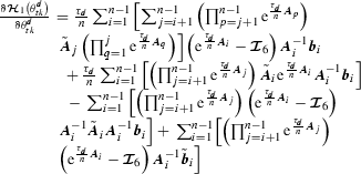• $\frac{\partial \varvec{\mathcal H}_{2}\left( \hat{\tau }_{k}, \theta ^{d}_{tk}\right) }{\partial \theta ^{d}_{tk}} = \frac{\partial \varvec{\mathcal J}_{2}\left( \hat{\tau }_{k}, \theta ^{d}_{tk}\right) }{\partial \theta ^{d}_{tk}}\varvec{A}_{n}^{-1}\varvec{b}_{n} - \left( \varvec{\mathcal J}_{2}\left( \hat{\tau }_{k},\theta ^{d}_{tk}\right) \right. \left. - \varvec{\mathcal I}_{6}\right) \varvec{A}_{n}^{-1}\left( \tilde{\varvec{A}}_{n} \varvec{A}_{n}^{-1}\varvec{b}_{n} + \tilde{\varvec{b}}_{n}\right)$.

Appendix 4

In this appendix, we demonstrate that $\frac{\partial {\mathcal L}_{1}\left( \varvec{\mathcal {P}}\left( \varvec{x}_{k}^{-}, \hat{\tau }_{k}, \theta ^{d}_{tk}\right) \right) }{\partial \hat{\tau }_{k}}$ $={\mathcal L}_{2}\left( \varvec{\mathcal {P}}\left( \varvec{x}_{k}^{-}, \hat{\tau }_{k}, \theta ^{d}_{tk}\right) \right)$.

First, the derivative of the function ${\mathcal L}_{1}\Big (\varvec{\mathcal {P}}\Big (\varvec{x}_{k}^{-}, \hat{\tau }_{k}, \theta ^{d}_{tk}\Big )\Big )$ with respect to $\hat{\tau }_{k}$ yields:

$$\begin{aligned}&\frac{\partial {\mathcal L}_{1} \left( \varvec{\mathcal {P}}\left( \varvec{x}_{k}^{-}, \hat{\tau }_{k}, \theta ^{d}_{tk}\right) \right) }{\partial \hat{\tau }_{k}}\nonumber \\&\quad = \frac{\partial {\mathcal L}_{1}\left( \varvec{\mathcal {P}}\left( \varvec{x}_{k}^{-}, \hat{\tau }_{k}, \theta ^{d}_{tk}\right) \right) }{\partial \varvec{\mathcal {P}}\left( \varvec{x}_{k}^{-}, \hat{\tau }_{k}, \theta ^{d}_{tk}\right) }\frac{\partial \varvec{\mathcal {P}}\left( \varvec{x}_{k}^{-}, \hat{\tau }_{k}, \theta ^{d}_{tk}\right) }{\partial \hat{\tau }_{k}}. \end{aligned}$$

(56)

Furthermore, according to “Appendix 3”, and as $\varvec{A}_{n}\varvec{\mathcal J}_{2}\left( \hat{\tau }_{k},\theta ^{d}_{tk}\right) = \varvec{\mathcal J}_{2}\left( \hat{\tau }_{k},\theta ^{d}_{tk}\right) \varvec{A}_{n}$, and taking into account that $\varvec{\mathcal G}_{1}\left( \varvec{x}_{k}^{-}, \theta ^{d}_{tk}\right) \! {=} \varvec{\mathcal J}_{1}\left( \theta ^{d}_{tk}\right) \varvec{h}\left( \varvec{x}_{k}^{-}\right) {+} \varvec{\mathcal H}_{1}\left( \theta ^{d}_{tk}\right)$, it follows that:

$$\begin{aligned}&\frac{\partial \varvec{\mathcal P}\left( \varvec{x}_{k}^{-}, \hat{\tau }_{k}, \theta ^{d}_{tk}\right) }{\partial \hat{\tau }_{k}}\nonumber \\&\quad = \varvec{\mathcal J}_{2}\left( \hat{\tau }_{k}, \theta ^{d}_{tk}\right) \left[ \varvec{A}_{n}\varvec{\mathcal G}_{1}\left( \varvec{x}_{k}^{-}, \theta ^{d}_{tk}\right) + \varvec{b}_{n}\right] , \end{aligned}$$

(57)

In addition, multiplying the first expression of the constrained controlled Poincaré map in (33) by the matrix $\varvec{A}_{n}$, and as $\varvec{A}_{n}\varvec{\mathcal H}_{2}\left( \hat{\tau }_{k},\theta ^{d}_{tk}\right) = \left( \varvec{\mathcal J}_{2}\left( \hat{\tau }_{k},\theta ^{d}_{tk}\right) -\varvec{I}_{6}\right) \varvec{b}_{n}$, we can prove that:

$$\begin{aligned}&\!\!\!\varvec{A}_{n}\varvec{\mathcal {P}}\left( \varvec{x}_{k}^{-}, \hat{\tau }_{k}, \theta ^{d}_{tk}\right) + \varvec{b}_{n}\nonumber \\&\!\!\!\quad = \varvec{\mathcal J}_{2}\left( \hat{\tau }_{k},\theta ^{d}_{tk} \right) \left[ \varvec{A}_{n} \varvec{\mathcal G}_{1} \left( \varvec{x}_{k}^{-}, \theta ^{d}_{tk}\right) + \varvec{b}_{n}\right] . \end{aligned}$$

(58)

Hence, according to (57) and (58), we deduce that:

$$\begin{aligned} \frac{\partial \varvec{\mathcal P}\left( \varvec{x}_{k}^{-}, \hat{\tau }_{k}, \theta ^{d}_{tk}\right) }{\partial \hat{\tau }_{k}} = \varvec{A}_{n}\varvec{\mathcal {P}}\left( \varvec{x}_{k}^{-}, \hat{\tau }_{k}, \theta ^{d}_{tk}\right) + \varvec{b}_{n}. \end{aligned}$$

(59)

Since $\varvec{x}_{k+1}^{-} = \varvec{\mathcal {P}}\left( \varvec{x}_{k}^{-}, \hat{\tau }_{k}, \theta ^{d}_{tk}\right)$, then we obtain:

$$\begin{aligned} \frac{\partial \varvec{\mathcal P}\left( \varvec{x}_{k}^{-}, \hat{\tau }_{k}, \theta ^{d}_{tk}\right) }{\partial \hat{\tau }_{k}} = \varvec{A}_{n}\varvec{x}_{k+1}^{-} + \varvec{b}_{n}. \end{aligned}$$

(60)

As a result, it states that:

$$\begin{aligned} \frac{\partial \varvec{\mathcal P}\left( \varvec{x}_{k}^{-}, \hat{\tau }_{k}, \theta ^{d}_{tk}\right) }{\partial \hat{\tau }_{k}} = \dot{\varvec{x}}_{k+1}^{-}. \end{aligned}$$

(61)

Hence, expression (56) is equivalent to:

$$\begin{aligned} \frac{\partial {\mathcal L}_{1}\left( \varvec{\mathcal {P}}\left( \varvec{x}_{k}^{-}, \hat{\tau }_{k}, \theta ^{d}_{tk}\right) \right) }{\partial \hat{\tau }_{k}} = \frac{\partial {\mathcal L}_{1}\left( \varvec{x}_{k+1}^{-}\right) }{\partial \varvec{x}_{k+1}^{-}}\dot{\varvec{x}}_{k+1}^{-}. \end{aligned}$$

(62)

In fact, relying on (10), we have ${\mathcal L}_{2}\left( \varvec{x}\right) = \frac{\partial {\mathcal L}_{1}\left( \varvec{x}\right) }{\partial \varvec{x}}\dot{\varvec{x}}$, then ${\mathcal L}_{2}\left( \varvec{x}_{k+1}^{-}\right) = \frac{\partial {\mathcal L}_{1}\left( \varvec{x}_{k+1}^{-}\right) }{\partial \varvec{x}_{k+1}^{-}}\dot{\varvec{x}}_{k+1}^{-}$. Hence, expression (62) is reformulated as follows:

$$\begin{aligned} \frac{\partial {\mathcal L}_{1}\left( \varvec{\mathcal {P}}\left( \varvec{x}_{k}^{-}, \hat{\tau }_{k}, \theta ^{d}_{tk}\right) \right) }{\partial \hat{\tau }_{k}} = {\mathcal L}_{2}\left( \varvec{\mathcal {P}}\left( \varvec{x}_{k}^{-}, \hat{\tau }_{k}, \theta ^{d}_{tk}\right) \right) . \end{aligned}$$

(63)

Finally, we stress that:

$$\begin{aligned} {\mathcal L}_{2}\left( \varvec{\mathcal {P}}\left( \varvec{x}_{k}^{-}, \hat{\tau }_{k}, \theta ^{d}_{tk}\right) \right) <0. \end{aligned}$$

(64)

Appendix 5

To achieve stabilization of the linearized controlled Poincaré map (34) by means of the control law (35), we define the following classical candidate Lyapunov function [34]:

$$\begin{aligned} V\left( \varDelta \varvec{x}_{k}^{-}\right) = {\varDelta \varvec{x}_{k}^{-}}^{T}\varvec{\mathcal S}\varDelta \varvec{x}_{k}^{-}, \end{aligned}$$

(65)

with $\varvec{\mathcal S}$ is a positive definite symmetric matrix.

Hence, the research for the matrix gain $\varvec{\mathcal K}$ lies in solving the following linear matrix inequality (LMI):

$$\begin{aligned} \left[ \begin{array}{cc} \varvec{\mathcal S} &{} {\mathcal D}\varvec{\mathcal P}_{\varvec{x}_{k}^{-}}^{*}\varvec{\mathcal S} + {\mathcal D}\varvec{\mathcal P}_{\theta ^{d}_{tk}}^{*} \varvec{\mathcal R} \\ \left( {\mathcal D}\varvec{\mathcal P}_{\varvec{x}_{k}^{-}}^{*}\varvec{\mathcal S} + {\mathcal D}\varvec{\mathcal P}_{\theta ^{d}_{tk}}^{*} \varvec{\mathcal R}\right) ^{T} &{} \varvec{\mathcal S} \end{array} \right] >0,\nonumber \\ \end{aligned}$$

(66)

with ${\mathcal D}\varvec{\mathcal P}_{\varvec{x}_{k}^{-}}^{*} = {\mathcal D}\varvec{\mathcal P}_{\varvec{x}_{k}^{-}}\left( \varvec{x}_{*}^{-}, \hat{\tau }_{*}, \theta ^{d}_{t*}\right) , {\mathcal D}\varvec{\mathcal P}_{\theta ^{d}_{tk}}^{*} = {\mathcal D}\varvec{\mathcal P}_{\theta ^{d}_{tk}}$ $\left( \varvec{x}_{*}^{-}, \hat{\tau }_{*}, \theta ^{d}_{t*}\right)$, and $\varvec{\mathcal R}=\varvec{\mathcal K}\varvec{\mathcal S}$.

In this LMI, the two unknown matrices are $\varvec{\mathcal S}$ and $\varvec{\mathcal R}$. The gain $\varvec{\mathcal K}$ of the control law (35) is then expressed by:

$$\begin{aligned} \varvec{\mathcal K} = \varvec{\mathcal R}\varvec{\mathcal S}^{-1}. \end{aligned}$$

(67)

References

McGeer, T.: Passive dynamic walking. Int. J. Robot. Res. 9(2), 62–68 (1990)
Goswami, A., Thuilot, B., Espiau, B.: A study of the passive gait of a compass-like biped robot: symmetry and chaos. Int. J. Robot. Res. 17, 1282–1301 (1998)
Garcia, M., Chatterjee, A., Ruina, A., Coleman, M.: The simplest walking model: stability, complexity, and scaling. ASME J. Biomech. Eng. 120, 281–288 (1998)
Wisse, M., Schwab, A.L., Van Der Helm, F.C.T.: Passive dynamic walking model with upper body. Robotica 22, 681–688 (2004)
Safa, A.T., Saadat, M.G., Naraghi, M.: Passive dynamic of the simplest walking model: replacing ramps with stairs. Mech. Mach. Theory 42(10), 1314–1325 (2007)
Rushdi, K., Koop, D., Wu, C.Q.: Experimental studies on passive dynamic bipedal walking. Robot. Auton. Syst. 62(4), 446–455 (2014)
Iqbal, S., Zang, X.Z., Zhu, Y.H., Zhao, J.: Bifurcations and chaos in passive dynamic walking: a review. Robot. Auton. Syst. 62(6), 889–909 (2014)
Asano, F.: Efficiency analysis of 2-period dynamic bipedal gaits. In: Proceedings of the IEEE/RSJ International Conference on Intelligent Robots and Systems, pp. 173–180. St. Louis, USA (2009)
Chyou, T., Liddell, G.F., Paulin, M.G.: An upper-body can improve the stability and efficiency of passive dynamic walking. J. Theor. Biol. 285, 126–135 (2011)
Iida, F., Tedrake, R.: Minimalistic control of biped walking in rough terrain. Auton. Robots 28(3), 355–368 (2010)
Gritli, H., Khraeif, N., Belghith, S.: A period-three passive gait tracking control for bipedal walking of a compass-gait biped robot. In: Proceedings of the International Conference on Communications, Computing and Control Applications, pp. 1–6. Hammamet, Tunisia (2011)
Spong, M.W., Bullo, F.: Controlled symmetries and passive walking. IEEE Trans. Autom. Control 50, 1025–1031 (2005)
Spong, M.W., Holm, J.K., Dongjun, L.: Passivity-based control of bipedal locomotion. IEEE Robot. Autom. Mag. 14(2), 30–40 (2007)
Gritli, H., Khraeif, N., Belghith, S.: Semi-passive control of a torso-driven compass-gait biped robot: bifurcation and chaos. In: Proceedings of the International Multi-conference on Systems, Signals and Devices, pp. 01–06. Sousse, Tunisia (2011)
Gritli, H., Belghith, S., Khraeif, N.: Intermittency and interior crisis as route to chaos in dynamic walking of two biped robots. Int. J. Bifurc. Chaos 22(3), Paper no. 1250056 (2012)
Gritli, H., Belghith, S., Khraeif, N.: Cyclic fold bifurcation and boundary crisis in dynamic walking of biped robots. Int. J. Bifurc. Chaos 22(10), Paper no. 1250257 (2012)
Chevallereau, C., Bessonnet, G., Abba, G., Aoustin, Y.: Bipedal Robots: Modeling, Design and Walking Synthesis Wiley-ISTE, 1st edn. Wiley, London (2009)
Li, Q., Yang, X.S.: New walking dynamics in the simplest passive bipedal walking model. Appl. Math. Model. 36(11), 5262–5271 (2012)
Li, Q., Tang, S., Yang, X.S.: New bifurcations in the simplest passive walking model. Chaos Interdiscip. J. Nonlinear Sci. 23, 043110 (2013)
Gritli, H., Khraeif, N., Belghith, S.: Cyclic-fold bifurcation in passive bipedal walking of a compass-gait biped robot with leg length discrepancy. In: Proceedings of the IEEE International Conference on Mechatronics, pp. 851–856. Istanbul, Turkey (2011)
Gritli, H., Khraeif, N., Belghith, S.: Period-three route to chaos induced by a cyclic-fold bifurcation in passive dynamic walking of a compass-gait biped robot. Commun. Nonlinear Sci. Numer. Simul. 17(11), 4356–4372 (2012)
Ott, E., Grebogi, C., Yorke, J.A.: Controlling chaos. Phys. Rev. Lett. 64(11), 1196–1199 (1990)
Kapitaniak, T.: Controlling Chaos: Theoretical and Practical Methods in Non-linear Dynamics. Academic Press, New York (1996)
Andrievskii, B.R., Fradkov, A.L.: Control of chaos: methods and applications. I. Methods. Autom. Remote Control 64(5), 673–713 (2003)
Andrievskii, B.R., Fradkov, A.L.: Control of chaos: methods and applications. II. Applications. Autom. Remote Control 65(4), 505–533 (2004)
Fradkov, A.L., Evans, R.J.: Control of chaos: methods and applications in engineering. Annu. Rev. Control 29(1), 33–56 (2005)
Fradkov, A.L., Evans, R.J., Andrievsky, B.R.: Control of chaos: methods and applications in mechanics. Philos. Trans. R. Soc. A 364(1846), 2279–2307 (2006)
Suzuki, S., Furuta, K.: Enhancement of stabilization for passive walking by chaos control approach. In: Proceedings of the 15th Triennial World Congress of the IFAC, pp. 133–138. Barcelona, Spain (2002)
Osuka, K., Sugimoto, Y.: Stabilization of quasi-passive-dynamic-walking based on delayed feedback control. In: Proceedings of International Conference on Control, Automation, Robotics and Vision, pp. 803–808. Singapore (2002)
Sugimoto, Y., Osuka, K.: Walking control of quasi passive dynamic walking robot ’Quartet III’ based on continuous delayed feedback control. In: Proceedings of the IEEE International Conference on Robotics and Biomimetics, pp. 606–611. Shenyang, China (2004)
Harata, Y., Asano, F., Taji, K., Uno, Y.: Efficient parametric excitation walking with delayed feedback control. Nonlinear Dyn. 67, 1327–1335 (2012)
Kurz, M.J., Stergiou, N.: An artificial neural network that utilizes hip joint actuations to control bifurcations and chaos in a passive dynamic bipedal walking model. Biol. Cybern. 93, 213–221 (2005)
Kurz, M.J., Stergiou, N.: Hip actuations can be used to control bifurcations and chaos in a passive dynamic walking model. J. Biomech. Eng. 129(2), 216–222 (2007)
Gritli, H., Khraeif, N., Belghith, S.: Chaos control in passive walking dynamics of a compass-gait model. Commun. Nonlinear Sci. Numer. Simul. 18(8), 2048–2065 (2013)
Parker, T.S., Chua, L.O.: Practical Numerical Algorithms for Chaotic Systems. Springer, New York (1989)
Hiskens, I.A., Pai, M.A.: Trajectory sensitivity analysis of hybrid systems. IEEE Trans. Circuits Syst. I 47(2), 204–220 (2000)
Author information
Authors and Affiliations
Corresponding author