
Abstract
The probability of the occurrence of urban flash floods has increased appreciably in recent years. Scientists have published various articles related to the estimation of the vulnerability of people and vehicles in urban areas resulting from flash floods. However, most published works are based on research performed using numerical models and laboratory experiments. This paper presents a novel approach that combines the implementation of image velocimetry technique (large-scale particle image velocimetry—LSPIV) using a flash flood video recorded by the public locally and the estimation of the vulnerability of people and vehicles to high water velocities in urban areas. A numerical one‐dimensional hydrodynamic model has also been used in this approach for water velocity characterization. The results presented in this paper correspond to a flash flood resulting on November 29, 2012, in the city of Asunción in Paraguay. During this flash flood, people and vehicles were observed being carried away because of high water velocities. Various sequences of the recorded flash flood video were characterized using LSPIV. The results obtained in this work validate the existing vulnerability criterion based on the effect of the flash flood and resulting high water velocities on people and vehicles.
1 Introduction
The probability of the occurrence of urban flash floods has increased appreciably in recent years (World Meteorological Organization, WMO 2009). Scientists and engineers (Wright-Mc Laughlin Engineers 1969; Rooseboom et al. 1986; Federal Emergency Management Agency 1979; Australia Institute of Engineers 1987; Témez 1992; Nanía 1999; Russo 2009; Engineers Australia 2010; Milanesi et al. 2015; Martínez-Gomariz et al. 2016) have published various articles related to specific problems generated by surface runoff during urban floods. These articles described the harmful effects of these floods on urban infrastructure including the negative effects on people and vehicles resulting from high water velocities. Quantifying the risk levels resulting from flash flooding is essential for planning and possible mitigation of these effects.
People safety during a flash flood may be compromised when persons are affected by flows where it is difficult to remain stable and standing, crossing a street, or operating a vehicle. The stability of persons while walking through high water velocities has been studied by various researchers since the late 1960s in order to determine peoples’ stability while walking through high water velocities. Although early studies evaluated people’s instability based only on the maximum water depth (Wright-Mc Laughlin Engineers 1969; Rooseboom et al. 1986), later and more recent studies showed that in urban areas it is possible to demonstrate that people’s stability is a function of water depth (h) and water velocity (v) (Federal Emergency Management Agency 1979; Australia Institute of Engineers 1987; Témez 1992; Nanía 1999; Russo 2009; Engineers Australia 2010; Milanesi et al. 2015; Martínez-Gomariz et al. 2016). The guide developed by the Australia Institute of Engineers (1987) and Engineers Australia (2010) established that in order to prevent people from being carried away on streets and surrounding runoff areas during a flash flood, the relation (v·h) should not exceed the value of 0.4 m2/s for children and 0.6 m2/s for adults. Milanesi et al. (2015) defined, using a numerical model, three vulnerability regions in an v–h plot shown later in this paper (drowning, toppling, and slipping by children and adults). All the studies referenced above, which analyzed people’s instability during floods, do not apply to vehicles and infrastructure.
Thresholds have been established to describe the negative effects of urban floods on vehicles. Xia et al. (2011) developed a formula for predicting the incipient vehicle velocities moved by the flow. The parameters required in that formula were estimated based on experimental data collected in the laboratory using a channel and reduced scale vehicle models (including scale effects).
To evaluate the flood risk in real scale, water velocity data are required. However, these data in urban areas are not commonly available and difficult to collect during flash flood events with high flow variability. Extreme flow conditions during flash floods make the use of intrusive measurement technologies, generally used in natural channels but not typically used to measure overland flow, such as current meters, Acoustic Doppler Velocimeter (ADV), and Acoustic Doppler Current Profilers (ADCPs), difficult because of the high risk in instrument operation and operator safety. In this work, an advanced experimental technique for water velocity measurements during urban floods is implemented. This technique consists of implementing at large-scale particle image velocimetry technique (LSPIV) that is in constant development (Fujita et al. 1998; Creutin et al. 2003; Muste et al. 2005, 2008; Hauet et al. 2009; Fujita et al. 2013; Le Coz et al. 2014; Le Boursicaud et al. 2016; Stumpf et al. 2016). Presently (2016), the LSPIV technique is implemented on digital videos recorded from an unmanned aerial vehicle (UAV) and from fixed digital cameras. The LSPIV technique allows, from the recorded digital images, the characterization of surface water velocity fields, and through further processing, the calculation of discharge. Implementing LSPIV insures operator safety because the video can be recorded from a safe area (out of the vulnerability region), and the distances required to analyze the images are measured after the flood event. More recent LSPIV applications include measurement of flash floods in mountain rivers (Patalano and García 2006; Le Coz et al. 2016) and flow in and around hydraulic structures (Patalano and García 2006). The technique has been adapted in this work for implementation with home videos, generally filmed by the public during urban flash flood events using various electronic devices (cell phones, digital cameras, and others). Corrections to the videos are needed because these videos are generally shaky because they are recorded with no tripod, and in most cases the cameras are panned on both sides. This paper presents the results of the implementation of LSPIV to a home video of a flash flood recorded on November 29, 2012, in the city of Asunción in Paraguay and the estimation of the vulnerability of people and vehicles based on stability criterion in flash floods proposed by previous work.
2 Materials and methods
The analyzed flash flood event that caused major damages in Asuncion, Paraguay occurred on November 29, 2012. This flash flood was generated by a large storm producing 95 mm of rainfall in 7 h (between 6:40 and 13:40). The maximum observed rainfall intensity during this event was approximately 115 mm/h. The hyetograph of this rainfall event is shown in Fig. 1. The hyetograph shows that the maximum rainfall occurred during the first hour of the event (45 mm).

Hyetograph recorded during the flood event of November 29, 2012 (time interval, Δt = 5 min)
The annual recurrence of this rainfall event is less than once every 5 years. Therefore, this event is not considered extraordinary. However, urban drainage systems are usually designed in Latin-American countries based on rainfall amounts with annual recurrences between 2 and 10 years (similar to the one described in this project). This recurrence value was estimated using the rainfall intensity, duration, and annual recurrence curve determined for Asuncion city, Paraguay.
During the analyzed flash flood event, a digital video was recorded at a 1280 by 720 pixels resolution and 30 frames per second by the public (an image of it is shown in Fig. 2) on Amancio Gonzalez Street 10 m from the intersection of Pirizal Street in Asuncion. During the flood, two vehicles were observed moving because of the water velocities (Fig. 3). Fortunately, no one was killed or injured at this site during the event.

Image of the digital video recorded by the public on Amancio Gonzalez Street (reference time = 0 s, being the starting time)

Part of the analyzed video in which cars were carried away (reference time = 240 s)
The surface water velocity at the site has been processed using the LSPIV technique following the experimental method described in Patalano and García (2006) and summarized as follows:
-
(a)
The amateur video was recorded with no tripod. Thus, the video is shaky and the operator is slightly panning the camera on both sides. Once extracted, the images were converted to grayscale and then digitally stabilized before image processing (Patalano and García 2006).
-
(b)
Images were processed with the MATLAB toolbox PIVLab (Thielicke and Stamhuis 2014), which processes the displacement field (in pixels) within pairs of images. The mean displacement field of the site was then calculated from the instantaneous displacement fields of the entire video.
-
(c)
Because of the oblique position of the camera, the mean displacement field of the region of interest had to be rectified. Thus, after the event, six distances between four control points (including diagonals) observed in the images have been surveyed 1 week after the flood event in order to orthorectify the displacement and process the real velocity field [m/s] knowing the time steps between the extracted images. This post-processing was completed using the toolbox RIVeR (Patalano and García 2006).
3 Results
The unrectified mean displacement vectors determined implementing LSPIV on images recorded during the event is shown in Fig. 4.

Mean unrectified surface water velocity field obtained after implementing LSPIV technique. Arrows represent surface water velocity vectors
The rectified mean surface water velocity field determined with the RIVeR MATLAB tool was calculated, and the following velocity cross sections were extracted (Fig. 5):

Surface water velocity cross sections extracted in three different cross sections with its corresponding location in the video
The flow in the upstream cross section (CS1) was uniformly distributed across the width of the street (Fig. 5). The maximum velocity in this cross section is about 3 m/s (in the center of the street), and the mean water velocity is about 2.3 m/s. The section CS2 corresponds to the location of the vehicle that causes a major contraction in the right side of the street. In CS2, the maximum velocity is 4.2 m/s and the mean water velocity is about 2.9 m/s. Finally, the downstream cross section (CS3) corresponds with the location of the maximum water velocities (5.4 m/s), and the mean water velocity is about 3.9 m/s.
In order to quantify water depths in Amancio Gonzales Street, the geometry of the street was surveyed after the flood event (see Fig. 7). The street and the sidewalks (on both sides) are unpaved. The lateral boundaries are mostly vertical, and the longitudinal slope of the street is 3.6%.
The water level never reaches the tire axis (except in cases where vehicles cause obstructions in the flow); thus, a water depth of 0.2 m over the sidewalk has been estimated (Fig. 6). Water depth is the variable in the analysis with the largest uncertainty as is discussed as follows: assuming that the tire is in an orthogonal plane to the direction of the camera and there is a lineal relation between the image pixels and the mean diameter of a tire, the water depth was estimated at 0.2 m ± 0.05 m.

Water depth estimation in the analyzed zone
The water depth in the place with maximum water velocity was determined using the water depth previously estimated based on the vehicle parked on the sidewalk (see Fig. 6) and the surveyed street cross section (see Fig. 7, indicating as water depth equal to 0 the water surface elevation).

Street section used to characterize the flood flow in CS1
Finally, the product of the measured water velocities (v) and water depths (h) was analyzed in order to evaluate the vulnerability to human stability (Table 1; Figs. 8, 12). Presently (2016), uncertainties in surface flow velocity measurements using LSPIV are being studied by different research groups (i.e., Hauet et al. 2009). Based on the authors’ experience, uncertainties on LSPIV surface flow velocity measurements errors are on the order of ±10%. In addition, uncertainties in water depth estimations performed in this work are on the order of 0.05 m. Thus, accounting for the uncertainties in the estimation of the vulnerability of people and vehicles based on stability criterion error, confidence intervals for the water velocity and water depth have been included in Figs. 8 and 12.

Stability regions defined by Milanesi et al. (2015) for adults (thin line) and children (thick line): (A) drowning, (B) toppling, and (C) slipping. Here, ρ = 1000 kg/m3 and there is null slope (horizontal terrain). Symbols represent the results obtained of the flow velocity measurements in the three cross sections of the analyzed video (filled circle CS1, filled diamond CS2, filled square CS3, open square CS1 sequence a, and open circle CS1 sequence b)
Engineers Australia (2010) limit for v·h (0.4 m2/s for children and 0.6 m2/s for adults) is significantly exceeded in cross sections CS2 and CS3 (Table 1).
The v–h values observed in this work at the three different cross sections are represented in Fig. 8. This plot also includes the regions defined by Milanesi et al. (2015) for drowning (A), toppling (B), and slipping (C) in the case of clear water (\( \rho = 1000\; {\text{kg}}/{\text{m}}^{3} \)) and horizontal terrain (null slope), for a child (thick line) and adult (thin line). This plot also defines thresholds that separate children from adults: low vulnerability (under the children line), medium vulnerability (between the children and adult lines), and high vulnerability (above the adult line). The values observed in the CS1 cross section are located in the region with medium vulnerability, and the instability mechanism is controlled by slipping. However, the values measured in CS2 and CS3 correspond to the high vulnerability region during the urban flood characterized in this work. Because, the velocity is so high (>4 m/s) for both CS2 and CS3, than the stability index (v·h) is not sensitive to the depth (h) (Fig. 8), provided depth (h) remains above ~0.1 m. Water flow depth is not a main factor at these two cross sections because the water velocity is so high in this region; and that is the reason of not taking into account sediment transport (erosion and deposition).
To complement the flow velocity field characterization, a numerical hydrodynamic model HEC RAS (USACE 2008) was implemented for the site. This model allows the user to perform a one-dimensional (steady flow) calculation, among other things if implemented.
To implement HEC RAS, first it was necessary to define roughness coefficients to simulate the flow resistance in the street and sidewalks. The roughness coefficients applied in this study (Manning coefficients n were used) are described below
-
1.
n value equal to 0.030 for the unpaved sidewalks (Chow 1959 for floodplain consisting of pastures).
-
2.
The n value of the street was calibrated using the maximum water velocity reached in the CS1 section in the center of the street (about 3 m/s) and the estimated water depth (0.2 m on the sidewalks). The value of n that represents the case study is 0.028 (in the literature, this value corresponds to an open channel excavated without vegetation; therefore, this value is acceptable because the street is unpaved).
The velocity distribution in the CS1 cross section simulated using the calibrated n roughness coefficients is shown in Fig. 9. The maximum velocity of about 3 m/s is reached near the center of the street and the water depth on the sidewalks is 0.2 m (Fig. 9) (both data were observed at the site).

Control section CS1 used to calibrate the n roughness coefficient of the hydrodynamic model HEC RAS
Three sequences of the video have been analyzed using the flow measurements and the calibrated HEC RAS model. The results were compared with the plot presented by Milanesi et al. (2015) and Xia et al. (2011). The selected sequences correspond to times when (a) people are standing on the sidewalk; (b) a man was carried away by the flow; and (c) vehicles were carried away by the flow.
-
(a)
During the first sequence of the video, people are standing on the right sidewalk of the flow (Fig. 10):
Fig. 10 
Sequence of the analyzed video when people are standing on the right sidewalk (reference time = 0 s)

Using the field measurements and the calibrated hydrodynamic model, a water velocity of 1.8 m/s and a water depth to 0.2 m was estimated at the site. Plotting the v–h values in Fig. 8, this flow condition corresponds to the low vulnerability region (there is no movement of the people affected by the flood) and region C (corresponding to the area where the instability mechanism is slipping).
-
(b)
In another part of the video, one man was trying to enter a vehicle. He was carried away by the flow. A colleague rescued him and a possible tragedy was avoided (Fig. 11).
Fig. 11 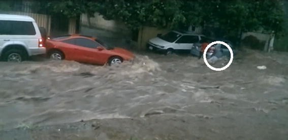
Part of the analyzed video in which a man (within the white circle) was carried away while he was trying to get into one vehicle (reference time = 50 s)

In this case, the person was located in the right side of the street near the sidewalk. Using field measurements and the calibrated hydrodynamic model, a water velocity of 2.9 m/s and a water depth equal to 0.33 m were estimated in this region. If these values are plotted in Fig. 8, this flow condition corresponds to the high vulnerability region (the drag on the man is clear) and the region C (corresponding to the area where the instability mechanism is the slipping).
-
(c)
In the last sequence of the video, two vehicles were carried away by the flow as it is shown previously in Fig. 3. In this case, the region where the cars were carried away coincides with sections CS2 and CS3. The water velocities in these cross sections range between 4.2 and 5.4 m/s, and the water depth ranges between 0.3 and 0.35 m (see Table 1).The velocity and water depth values observed in this work (Fig. 12) for two of the analyzed cross sections (CS2 and CS3) in the v–h stability plot prepared by Xia et al. (2011) for two vehicle types and for different vehicle orientation angles (0 and 180°) aligned parallel to the water velocity vector and 90° being normal to this vector.

The values observed in CS2 and CS3 indicated that the measurements are above every threshold defined by Xia et al. (2011). The results reached in the analyzed video indicate that the vehicle stability thresholds are always exceeded. During the recorded event and because of the high water velocities reached by the flow, large movements of large vehicles were observed. The vehicles move in the region of largest values of v–h that corresponds to the high vulnerability zone defined by Xia et al. (2011) for vehicles.
4 Summary and conclusions
In this work, the water velocities in one street of Asuncion, Paraguay, are experimentally determined during an urban flash flood using an advanced experimental technique available for non-contact measurements of large-scale surface water velocities: LSPIV. During this urban flood and because of the high velocities measured, people slipping and carried away and appreciable movements of large vehicles were observed.
A one‐dimensional numerical hydrodynamic model was also used for the velocity characterization during flood events. Based on the correct analysis of the video, valuable hydraulic data can be computed and used for the calibration of the hydrodynamic model.
Various sequences of the video were characterized taking into account the vulnerability criterion based on the stability of people and vehicles in flash floods proposed by Milanesi et al. (2015) and Xia et al. (2011), respectively. The maximum measured values of (v·h) always exceed the vulnerability limits of people defined in previous works (Engineers Australia 2010) to prevent people from being carried away in streets and other areas of runoff during a flash flood. It has been shown that if people remained on the sidewalk, they were in a region of low vulnerability; whereas if they were in the street they were in area a region of high vulnerability. For both cases, the associated instability mechanism for people is slipping. In addition, it was shown that the flow contraction caused by vehicles on the right bank (right side of the street) significantly increases the vulnerability and risk of the analyzed situation.
In order to analyze the stability thresholds for vehicles, the criterion proposed by Xia et al. (2011) was used. Using the measurements collected in Xia’s study, it was shown that downstream of the flow contraction, the vehicle’s instability limit is exceeded and corresponds to the appreciable movement of vehicles observed in the video.
This work illustrates the great potential of citizen science initiatives for improving flood risk assessment as valuable hydraulic data can be computed using messages, photographs and movies produced by citizens. Nowadays, new communication and digital image technologies have enabled the public to produce large quantities of flood observations and share them through social media. The authors of this paper are working in citizen science projects in Argentina focused in the generation of crowd-sourced data for flood hydrology. In addition to citizen science initiatives, the authors are also evaluating the application of near infrared surveillance camera networks in urban areas to quantify flood vulnerability in real time using LSPIV.
Abbreviations
- LSPIV:
-
Large-scale particle image velocimetry
References
Australia Institute of Engineers (1987) Australian rainfall and runoff, vol 1&2. (Ed: Pilgrim, D.H.) Institution of Engineers, Australia
Chow VT (1959) Open-channel hydraulics. McGraw-Hill, New York, p 680
Creutin J-D, Muste M, Bradley A, Kim SC, Kruger A (2003) River gauging using PIV techniques: a proof of concept experiment on the Iowa River. J Hydrol 277(3–4):182–194
Engineers Australia (2010) Australian rainfall and runoff revision projects. PROJECT 10 appropriate safety criteria for people. STAGE 1 REPORT P10/S1/006. April 2010
Federal Emergency Management Agency (FEMA) (1979) The floodway: a guide for community permit officials. EEUU
Fujita I, Muste M, Kruger A (1998) Large-scale particle image velocimetry for flow analysis in hydraulic engineering applications. J Hydraul Res 36(3):397–414
Fujita I, Kunita Y, Tsubaki R (2013) Image analysis and reconstruction of the 2008 Toga River flash flood in an urbanized area. Aust J Water Resour 16(2):12
Hauet A, Muste M, Ho HC (2009) Digital mapping of riverine waterway hydrodynamic and geomorphic features. Earth Surf Proc Land 34(2):242–252
Le Boursicaud R, Pénard L, Hauet A, Thollet T, Le Coz J (2016) Gauging extreme floods on YouTube: application of LSPIV to home movies for the post-event determination of stream discharges. Hydrol Process 30:90–105
Le Coz J, Magali Jodeau, Hauet A, Marchand B, Le Boursicaud R (2014) Image-based velocity and discharge measurements in field and laboratory river engineering studies using the free FUDAA-LSPIV software. River Flow, Lausanne
Le Coz J, Patalano A, Collins D, Guillén NF, García CM, Smart GM, Bind J, Chiaverini A, Le Boursiqueau R, Dramais G, Braud I (2016) Crowd-sourced data for flood hydrology: feedback from recent citizen science projects in Argentina, France and New Zealand. J Hydrol. Available online 26 July 2016, ISSN 0022-1694, http://dx.doi.org/10.1016/j.jhydrol.2016.07.036. (http://www.sciencedirect.com/science/article/pii/S0022169416304668)
Martínez-Gomariz E, Gómez M, Russo B (2016) Experimental study of the stability of pedestrians exposed to urban pluvial flooding. Nat Hazards 1–20
Milanesi L, Pilotti M, Ranzi R (2015) A conceptual model of people’s vulnerability to floods. Water Resour Res 51:182–197. doi:10.1002/2014WR016172
Muste M, Schöne J, Creutin J-D (2005) Measurement of free-surface flow velocity using controlled surface waves. Flow Meas Instrum 16(1):47–55
Muste M, Fujita I, Hauet A (2008) Large-scale particle image velocimetry for measurements in riverine environments. Water Resour Res 44:1–14
Nanía LS (1999) Metodología numérico experimental para el análisis del riesgo asociado a la escorrentía pluvial en una red de calles. Tesis doctoral. Universitat Politècnica de Catalunya, Barcelona, España
Patalano A, García CM (2006) RIVeR—towards affordable, practical and user-friendly toolbox for large scale PIV and PTV techniques. In: IAHR RiverFlow Conference, St. Louis, Missouri, USA
Rooseboom A, Basson MS, Loots CH, Wiggett JH, Bosman J (1986) Manual on road drainage, 2nd edn. National Transport Commission, Chief Director of National Road, Republic of South Africa
Russo B (2009) Design of surface drainage systems according to hazard criteria related to flooding of urban areas. Tesis doctoral. Universitat Politècnica de Catalunya, Barcelona, España
Stumpf A, Augereau E, Delacourt C, Bonnier J (2016) Photogrammetric discharge monitoring of small tropical mountain rivers: a case study at Rivière des Pluies, Réunion Island. Water Resour Res 52(6):4550–4570
Témez JR (1992) Control del desarrollo urbano en las zonas inundables. Monografías del Colegio de Ingenieros de Caminos, Canales y Puertos, vol 10, pp 105–115. Madrid, Spain
Thielicke W, Stamhuis EJ (2014) PIVlab—towards user-friendly, affordable and accurate digital particle image velocimetry in MATLAB. J Open Res Softw 2(1):e30. doi:10.5334/jors.bl
USACE [US Army Corps of Engineers] (2008) HEC-RAS Version 4.1. Davis, CA Institute for Water Resources, Hydrologic Engineering Center
WMO [World Meteorological Organization] (2009) Flood management in a changing climate. APFM technical document no. 9, Flood management tools series, associated programme on flood management (WMO), Geneva. Switzerland. www.apfm.info/pdf/ifm_tools/Tools_FM_in_a_changing_climate.pdf
Wright-Mc Laughlin Engineers (1969) Urban drainage and flood control district, vol 861. Denver, Colorado, USA
Xia J, Teo FY, Lin B, Falconer RA (2011) Formula of incipient velocity for flooded vehicles. Nat Hazards 58(1):1–14
Acknowledgements
The authors acknowledge Angel M. Martin, Jr., USGS retired, for his technical edit and constructive comments on the manuscript; Kevin A. Oberg, USGS—Office of Surface Water, for helping in the final edition of this work; and two anonymous reviewers provided useful comments and suggestions for improving the manuscript.
Author information
Authors and Affiliations
Corresponding author
Rights and permissions
About this article

Cite this article
Guillén, N.F., Patalano, A., García, C.M. et al. Use of LSPIV in assessing urban flash flood vulnerability. Nat Hazards 87, 383–394 (2017). https://doi.org/10.1007/s11069-017-2768-8
Received:
Accepted:
Published:
Issue Date:
DOI: https://doi.org/10.1007/s11069-017-2768-8