Dynamics modeling and analysis of a flexible-base space robot for capturing large flexible spacecraft

Abstract

Space robots are in huge demand due to the rapid growth of their service targets, i.e., spacecraft. There are generally large flexible components on spacecraft, such as antenna reflectors and solar paddles. Due to the vibratility of their structure, it is challenging for a space robot with flexible appendages (the base is then called flexible-base) to capture and repair the large flexible spacecraft. After capturing, the two spacecraft with flexible appendages are connected by a space manipulator, and a compounded system is formed. In this paper, we developed a dynamic model and a closed-loop simulation system, to provide a means to verify path planning and control algorithms. Initially, the dynamic characteristics of different capturing stages (preimpact and post-impact) were analyzed. The topologies of a flexible-base space robot and the compounded system were described based on incidence and channel matrices. Secondly, the recursive dynamics was formulated and resolved by an effective numerical method. The modeling was verified by Adams’ model. Thirdly, we implemented a dynamics calculation block in Matlab/Simulink environment using the S-function package for the C program, and developed a closed-loop simulation system, which was composed of the Planning and Controller, the Multibody Dynamic, and the 3D Display modules. Finally, based on the simulation system, two typical missions—target berthing and on-orbital manipulation of the target along a circle, were simulated and evaluated. Dynamics analysis results presented some useful rules for the path planning and control to suppress the vibration of the flexible structure.

1 Introduction

Robotic systems are expected to play an increasingly important role in future space activities, such as repairing, upgrading, refueling, and reorbiting spacecraft [1–4]. These technologies could potentially extend the life of satellites, enhance the capability of space systems, reduce operation costs, and clean up the increasing space debris. The autonomous target capturing, which has been successfully demonstrated by the Engineering Test Satellite VII (ETS-VII) [5] and Orbital Express [6], is the key to on-orbit servicing. Unlike on the earth, space operations require the ability to work in the unstructured environment [7]. Some autonomous behaviors are necessary to perform complex and difficult tasks in space. Yoshida and Umetani developed on-line control scheme with vision feedback, using Generalized Jacobian Matrix (GJM) concept for motion control and Guaranteed Workspace (GWS) for path planning [8]. Yoshida et al. also proposed an impedance matching method to capture a noncooperative target [9], and a possible control sequence to capture a tumbling target [10]. Papadopoulous et al. studied the dynamics and control of a multiarm space robot involved in chase and capture operations of satellites [11]. Nagamatsu et al. designed a control system for the autonomous capture of a target satellite in space using a predictive trajectory based on the target satellite dynamics [12]. McCourt and Silva investigated the use of model-based predictive control for the capture of a multi-DOF object that moves in a somewhat arbitrary manner [13]. Xu et al. also proposed autonomous path planning and control methods to capture a noncooperative target based on the binocular stereo vision [14]. Recently, Aghili presented a combined prediction and motion-planning scheme for robotic capturing of a drifting and tumbling object with unknown dynamics using visual feedback [15]. For the above works, the space robot and the target satellite are assumed to be multirigid systems, and the dynamics coupling [16] between the base and the manipulator are the main factor considered for path planning and control.

Actually, there exist flexible components, including flexible links, joints, etc., on space robots since space applications require light-weight designs. Dwivedy and Eberhard conducted a comprehensive review of the literature on the dynamics analysis and control of flexible manipulators [17]; the flexible links or/and flexible joints are considered. Ma et al. [18] developed a software package—MDSF to model and simulate general robotic systems with flexible structures. Talebi presented an approach for dynamics modeling of flexible-link manipulators using artificial neural networks. It is applied to the Space Station Remote Manipulator System (SSRMS) [19]. Mohan and Saha proposed a recursive, numerically stable simulation algorithm for serial robots with flexible links [20]. Sabatini et al. designed active damping strategies to reduce the structural vibrations of a space manipulator with flexible links during its on orbit operations [21]. Masoudi and Mahzoon studied a free-floating space robot with four linkages, two flexible arms, and a rigid end-effector that are mounted on a rigid spacecraft [22]. Zarafshan and Moosavian derived the dynamic equations of a space robot with a flexible panel and a planar dual-arm system is taken as the example [23, 24]. Recently, the construction of large space structures, such as solar power stations and space telescopes, attracted the interest of scholars. Boning and Dubowsky presented a coordinated control method of space robot teams for the on-orbit assembly of large flexible space structures [25, 26]. The robots (each robot is mainly composed of rigid components), acting as force sources, maneuver and assemble these large, flexible space structures while minimizing vibration.

However, few literatures addressed the dynamics modeling and control of a flexible-base space robot capturing a large flexible satellite. In fact, a spacecraft, such as a GEO satellite for broadcasting, communications, weather forecasting and so forth, is growing in size to meet ever more demanding mission requirements. Large flexible components such as antenna reflectors and solar paddles are inevitably mounted on the spacecraft. For example, the Japanese Engineering Test Satellite VIII (ETS-VIII) has a size of 40×37 m and a mass of 3000 kg [27]. Two large deployable reflectors are appended in the roll axis direction, and a pair of solar paddles rotates around the pitch axis at a rate of 360^o/day so that they continually face the sun. The modeling of the large flexible spacecraft on orbit is complex [28]. On the other hand, a space robot used to complete the on-orbit servicing tasks has also generally flexible solar panels. It is very challenging for such a space robot to capture and repair these large flexible satellites for two reasons. First, the structure flexibilities (including the flexibilities of the space robot and the target satellite) will easily cause vibration while the space robot capturing and manipulating the target. The generated vibration is difficult to be reduced since there does not exist atmospheric damping in the orbit and the structure damping is very little. Second, a space robot is designed to be as light as possible for saving manufacturing and launching costs, so the geometry and inertial parameters (mass and inertia) of the target satellite are much larger than those of the space robot. After the target is captured or released, the mass properties of the space system will change dramatically.

In order to supply a means to analyze the design of the space robot system, and verify the key path planning and control algorithms, we derived the dynamics equations of a flexible-base space robot, and the compounded system after it captures a large flexible spacecraft. Based on the derived dynamic equations, a closed-loop control simulation system is developed. The absolute motion of the base is described as a 6-DOF virtual hinge between the base and the inertial frame. Two types of kinematic relations between adjacent bodies, including rigid-rigid and rigid-flexible bodies, are established, respectively. Then the recursive equations are formulated and an effective numerical calculus method is used to solve it. The dynamics modeling and resolving code is programmed using C language, and verified by comparing the calculation results with those of Adams virtual prototype model under the same condition. Furthermore, the dynamics calculation block is implemented in Matlab/Simulink environment, and the closed-loop simulation system is developed. Using this system, dynamics analysis of two typical missions—target berthing and on-orbital manipulating of the target along a circle are performed.

This paper is organized as follows: Sect. 2 introduces the on-orbit system used for large flexible spacecraft and discusses the dynamic characteristics for different stages during the target capturing. Section 3 derives the recursive formulation for the rigid-flexible coupling dynamics of a flexible-base space robot capturing large flexible spacecraft. In Sect. 4, the dynamic equations are then resolved using numerical integration method, programmed in C language and verified by comparing with Adams software. Section 5 develops the closed-loop control simulation system in Matlab/Simulink environment. Then the dynamics analysis of two typical missions using different path planning methods is performed in Sect. 6. Finally, conclusions are presented in Sect. 7. The last section contains the Acknowledgements.

2 The on-orbit servicing system and dynamics characteristics

The target to be serviced is assumed a GEO spacecraft. Here, a Chinese communication satellite of the DFH-4 platform, the third generation of China GEO platform, is taken as the example. The main body of the DFH-4 satellite is a box-form structure with the size of 2.36 m×2.1 m×3.6 m. The satellite has large deployable solar wings and large deployable communications antennas with aperture of 3.0 m×2.2 m, which are folded when the satellite is launched and deploy when it enters the orbit. The wing span reaches 33.0 m and the height is 6.4 m. The satellite has 5200 kg lift off mass and a 15-year designed lifetime [29].

SINOSAT-2, launched in 2006, is the first application of DFH-4 platform. Unfortunately, a very severe case happened after it reached the GEO orbit successfully. It encountered three mechanical malfunctions: (1) The +Y solar wing fails to deploy; (2) The +X communication antenna fails to deploy, and (3) The −X communication antenna fails to deploy.

To resume the normal function of the communication satellite, theses malfunctions must be resolved. We designed a space robot to perform the on-orbit servicing mission [30]. It is mainly composed of a 7-DOF (Degree of Freedom) manipulator with two hand-eye cameras and a replaceable end-effector, a 2-DOF docking and latching mechanism (DLM) and three target support brackets (TSB), etc. The large flexible spacecraft and the space robot are shown as Fig. 1.

Fig. 1

The large flexible spacecraft and the designed space robot

The on-orbit capturing and manipulation of the target is the key of the on-orbit servicing mission. The capture process includes three specific phases [31]: the preimpact phase, the contact/impact phase, and the post-impact phase. During the preimpact phase, the space manipulator’s end-effector tracks and approaches the target spacecraft to its capturing box. In the impact phase, the contact/impact between the manipulator hand and the object is established, and a force impulse is generated. After the space robot captures the target successfully (i.e., post-impact phase), a compounded system is formed, which includes the space robot and the grasped target. At any stage, inappropriate robotic arm movement will cause the flexible spacecraft to vibrate for a long time. The vibration is highly coupled with the motion of the space manipulator and the base, which will not only lead to the failure of the servicing tasks, but also destroy the entire system.

Corresponding to different stages, there are different dynamic characteristics. Before the target is captured (i.e., precapture stage), the target spacecraft and the space robot are separated from each other. The former is actually a system composed of a central rigid body and two flexible solar paddles. It moves according to the principles of celestial mechanics and the initial conditions, such as free-floating, tumbling, and so on. For the space robot, it autonomously approaches the target under the visual serving control. It can be described as a dynamics system composed of a flexible base (a central rigid body + two flexible solar paddles) and a 7DOF rigid manipulator. It is a typical rigid-flexible coupling multibody dynamics system. After the space robot captures the target successfully (i.e., the post-impact phase), the space robot and the target form a new compounded system. Both the end points of the new system are flexible spacecrafts (i.e., flexible base of the space robot and the flexible target); they are connected by a rigid manipulator. That is to say, the dynamics states of the compounded system are determined by those of the flexible base, multirigid body (7-DOF rigid manipulator), and the flexible target. In the following contents, we focus on the modeling of the space system for preimpact and post-impact stages, shown as Fig. 2.

Fig. 2

Different dynamic characteristics of pre and post-impact stages

3 Dynamics modeling of flexible-base space robot for pre and post-impact stages

The designed space robotic system (the chaser spacecraft) used for the on-orbit servicing mission is shown as Fig. 3. It is composed of a central rigid body (called robot base), two flexible solar paddles, and a 7-DOF serial manipulator (called space manipulator). Each solar paddle is connected to the robot base through a rotating hinge with one degree of freedom. The hinges rotate according to the sun vector so that the solar paddles continually face the sun and they can provide as much energy as possible. Hence, the space robot can be described using 11 bodies (including the inertial frame) and 10 hinges. The bodies are denoted as follows:

• (1) B₀: the inertial body, a virtual body fixed in the inertial space;

• (2) B₁: the robot base, a central rigid body;

• (3) B₂–B₃: the flexible solar wings of the space robot;

• (4) B₄–B₁₀: the links of the space manipulator. B₄–B₁₀ are respectively the 1st–7th link of the 7-DOF manipulator; all are rigid bodies.

Fig. 3

The flexible-base space robot for the precapture stage

After capturing, the target satellite is locked to the end-effector of the space manipulator. Then a new system, called compounded system or compounded system, is formed. The compounded system consists of two parts: flexible-base space robot and flexible target spacecraft, as shown in Fig. 4. The target spacecraft is also composed of a central rigid body (called target base and denoted as $\mathrm{B}_{10}'$) and a pair of flexible solar wings (denoted as B₁₁ and B₁₂, respectively). The target base $\mathrm{B}_{10}'$ is fixed to the end-effector of the space manipulator, i.e., B₁₀. Thus, these two rigid bodies can be regarded as a rigid body and denotes as $\hat{\mathrm{B}}_{10}$.

Fig. 4

The compounded system after capturing

3.1 The definition of the coordinate systems

3.1.1 The inertial frame of reference

For the modeling of a multibody dynamic, the inertial frame of reference (also called inertial reference frame or inertial frame) is used to determine the absolute motion of each body. The inertial frame is denoted as O₀ x ₀ y ₀ z ₀, whose origin is Point O₀, three axes are O₀ x ₀, O₀ y ₀, O₀ z ₀, respectively. The inertial frame O₀ x ₀ y ₀ z ₀ is fixed at the virtual rigid body B₀.

3.1.2 The coordinate system of the space robot

The space robot is a hybrid rigid-flexible system, i.e., it is composed of rigid and flexible bodies. The centroid frame and floating coordinate system are respectively used as the body-fixed frames of the rigid and flexible bodies. Figure 5 shows the coordinate systems for the robot base and its solar wings. Frame O₁ x ₁ y ₁ z ₁ is the centroid frame of B₁. The origin is located in the center of mass (CM) of B₁. Frames O₂ x ₂ y ₂ z ₂ and O₃ x ₃ y ₃ z ₃ are respectively the floating coordinate systems of B₂ and B₃ (they are flexible bodies). Their origins, i.e., O₂ and O₃, are located at the hinges between the solar paddles (B₂ and B₃) and the central rigid body B₁. The initial orientations of O₂ x ₂ y ₂ z ₂ and O₃ x ₃ y ₃ z ₃ are assumed to the same as frame O₁ x ₁ y ₁ z ₁. The body-fixed frames of the space manipulator are defined as Fig. 6 (when the joint angles are all zeros). The origins are located in the centroid of each link of the manipulator. The z-axes of the frames are the rotation directions of corresponding joints. The zero configuration of the space robot is shown as Fig. 7.

Fig. 5

The coordinate system of the space base and its solar wings

Fig. 6

The body-fixed frames of the space manipulator

Fig. 7

The zero configuration of the space robot

3.1.3 The coordinate system of the target spacecraft

The coordinate systems of the target spacecraft are shown in Fig. 8, where $\mathrm{O}_{10}'x_{10}'y_{10}'z_{10}'$ is the centroid frame of $\mathrm{B}_{10}'$, O₁₁ x ₁₁ y ₁₁ z ₁₁ and O₁₂ x ₁₂ y ₁₂ z ₁₂ are respectively the floating coordinate systems of bodies B₁₁ and B₁₂ (they are flexible bodies). Their origins, i.e., O₁₁ and O₁₂, are located at the hinges between the solar paddles (B₁₁ and B₁₂) and the central rigid body $\mathrm{B}_{10}'$. A frame, denoted as O_nozzle x _nozzle y _nozzle z _nozzle, is defined to represent the apogee engine nozzle. Its origin is located in the circle center of the bottom surface of the apogee engine nozzle. The x-, y-, z-axis are parallel to the corresponding axis of Frame $\mathrm{O}_{10}'x_{10}'y_{10}'z_{10}'$. For the capturing or docking missions, the nozzle frame is taken as the target frame of visual measurement and navigation algorithm for the space robot.

Fig. 8

The coordinate system of the target spacecraft

3.2 System topology structure

3.2.1 The topology of the space robot before capturing

The topology diagram of the space robot system before capturing is shown in Fig. 9. The hinges are denoted as follows:

• (1) H₁: a 6-DOF virtual hinge between B₀ and B₁, representing the free motion of the robot base with respect to the inertial frame;

• (2) H₂–H₃: 1-DOF rotating hinges, representing the rotation motion between the solar wings B₂, B₃ and the robot base B₁;

• (3) H₄–H₁₀: 1-DOF rotating hinges. They are sequentially the 1st–7th joint of the 7-DOF manipulator.

Fig. 9

The topology of the space robot

The topology of a mechanical system can be described using an incidence matrix and a channel matrix [32]. For the space robot shown in Fig. 9, the incidence matrix S _Rbt is (the missing elements are zeros; hereinafter the same in this paper):

$$ \mathbf{S}_{\mathrm{Rbt}} = \left [ \begin{array}{c@{\quad}c@{\quad}c@{\quad}c@{\quad}c@{\quad}c@{\quad}c@{\quad}c@{\quad}c@{\quad}c} 1 & 0 & 0 & 0 & 0 & 0 & 0 & 0 & 0 & 0 \\ - 1 & 1 & 1 & 1 & 0 & 0 & 0 & 0 & 0 & 0 \\ & - 1 & 0 & 0 & 0 & 0 & 0 & 0 & 0 & 0 \\ & & - 1 & 0 & 0 & 0 & 0 & 0 & 0 & 0 \\ & & & - 1 & 1 & 0 & 0 & 0 & 0 & 0 \\ & & & & - 1 & 1 & 0 & 0 & 0 & 0 \\ & & & & & - 1 & 1 & 0 & 0 & 0 \\ & & & & & & - 1 & 1 & 0 & 0 \\ & & & & & & & - 1 & 1 & 0 \\ & & & & & & & & - 1 & 1 \\ & & & & & & & & & - 1 \end{array} \right ] \in \mathbf{R}^{11 \times 10} $$

(1)

The row and column numbers of S _Rbt are respectively the indexes of body and hinge. The value of the ith row and jth column element is defined as follows:

$$ S_{ij} = \left \{ \begin{array}{l@{\quad}l} 1, & i = i^{ +} ( j ) \\ - 1, & i = i^{ -} ( j ) \\ 0, & i \ne i^{ +} ( j ),i^{ -} ( j ) \end{array} \right .\quad ( i = 0,1, \ldots,10;j = 1, \ldots,10 ) $$

(2)

where i ⁺(j), i ⁻(j) represents the numbers of the inscribed and external body of hinge H _j . For the topology shown in Fig. 9, the values of i ⁺(j) and i ⁻(j) are as follows:

$$\begin{aligned} & i^{ +} ( j ) = \left \{ \begin{array}{l@{\quad}l} 0, & j = 1 \\ 1, & j = 2,3,4\\ j - 1, & j = 5, \ldots,10 \end{array} \right . \end{aligned}$$

(3)

$$\begin{aligned} & i^{ -} ( j ) = j\quad ( j = 1, \ldots,10 ) \end{aligned}$$

(4)

The channel matrix T _Rbt is

$$ \mathbf{T}_{\mathrm{Rbt}} = \left [ \begin{array}{c@{\quad}c@{\quad}c@{\quad}c@{\quad}c@{\quad}c@{\quad}c@{\quad}c@{\quad}c@{\quad}c} - 1 & - 1 & - 1 & - 1 & - 1 & - 1 & - 1 & - 1 & - 1 & - 1 \\ & - 1 & 0 & 0 & 0 & 0 & 0 & 0 & 0 & 0 \\ & & - 1 & 0 & 0 & 0 & 0 & 0 & 0 & 0 \\ & & & - 1 & - 1 & - 1 & - 1 & - 1 & - 1 & - 1 \\ & & & & - 1 & - 1 & - 1 & - 1 & - 1 & - 1 \\ & & & & & - 1 & - 1 & - 1 & - 1 & - 1 \\ & & & & & & - 1 & - 1 & - 1 & - 1 \\ & & & & & & & - 1 & - 1 & - 1 \\ & & & & & & & & - 1 & - 1 \\ & & & & & & & & & - 1 \end{array} \right ] \in \mathbf{R}^{10 \times 10} $$

(5)

The row and column numbers of T _Rbt are respectively the indexes of hinge and body. The value of the jth row and ith column element is defined as follows:

$$ T_{ji} = \left \{ \begin{array}{l@{\quad}l} 1, & \mbox{if } \mathrm{H}_{j}\ \mathrm{is}\ \mbox{on } \mathrm{the}\ \mathrm{path}\ \mbox{from } \mathrm{B}_{0}\ \mathrm{to} \mathrm{B}_{i},\ \mathrm{pointing}\ \mathrm{to}\ \mathrm{B}_{0} \\ - 1, & \mbox{if } \mathrm{H}_{j}\ \mathrm{is}\ \mbox{on } \mathrm{the}\ \mathrm{path}\ \mbox{from } \mathrm{B}_{0}\ \mathrm{to} \mathrm{B}_{i},\mbox{and}\ \mathrm{back}\ \mathrm{to}\ \mathrm{B}_{0}\quad ( i,j = 1, \ldots,10 ) \\ 0, & \mbox{if } \mathrm{H}_{j}\ \mathrm{is}\ \mathrm{not}\ \mbox{on }\ \mathrm{the}\ \mathrm{path}\ \mbox{from } \mathrm{B}_{0}\ \mathrm{to}\ \mathrm{B}_{i} \end{array} \right . $$

(6)

3.2.2 The topology of the compounded system after capturing

The topology diagram of the compounded system after capturing is shown in Fig. 10. The target base, i.e., $\mathrm{B}_{10}'$, is fixed to the end-effector of the space manipulator, i.e., B₁₀, and a new rigid body $\hat{\mathrm{B}}_{10}$ is formed. Hinges H₁₁ and H₁₂ are both 1-DOF rotation joints, connecting the solar wings to body $\hat{\mathrm{B}}_{10}$.

Fig. 10

The topology of the compounded system

The incidence matrix of the compounded system is

$$ \mathbf{S}_{\mathrm{CRS}} = \left [ \begin{array}{c@{\quad}c@{\quad}c} \mathbf{S}_{\mathrm{Rbt}} & \vdots & \mathbf{S}_{12} \\ \cdots & \cdots & \cdots \\ \mathbf{S}_{21} & \vdots & \mathbf{S}_{22} \end{array} \right ] \in \mathbf{R}^{13 \times 12} $$

(7)

where S _Rbt is given in (1), and (O _m×n denotes a m×n zeros matrix):

$$\begin{aligned} & \mathbf{S}_{12} = \left [ \begin{array}{c@{\quad}c} \mathbf{O}_{10 \times 1} & \mathbf{O}_{10 \times 1} \\ 1 & 0 \end{array} \right ] \in \mathbf{R}^{11 \times 2} \end{aligned}$$

(8)

$$\begin{aligned} & \mathbf{S}_{21} = \mathbf{O}_{2 \times 10} \end{aligned}$$

(9)

$$\begin{aligned} & \mathbf{S}_{22} = \left [ \begin{array}{c@{\quad}c} - 1 & 1 \\ 0 & - 1 \end{array} \right ] \in \mathbf{R}^{2 \times 2} \end{aligned}$$

(10)

The channel matrix of the compounded system is

$$ \mathbf{T}_{\mathrm{CRS}} = \left [ \begin{array}{c@{\quad}c@{\quad}c} \mathbf{T}_{\mathrm{Rbt}} & \vdots & \mathbf{T}_{12} \\ \cdots & \cdots & \cdots \\ \mathbf{T}_{21} & \vdots & \mathbf{T}_{22} \end{array} \right ] \in \mathbf{R}^{12 \times 12} $$

(11)

where T _Rbt is given in (5), and

$$\begin{aligned} &\mathbf{T}_{12} = \left [ \begin{array}{c@{\quad}c@{\quad}c@{\quad}c@{\quad}c@{\quad}c@{\quad}c@{\quad}c@{\quad}c@{\quad}c} - 1 & 0 & 0 & - 1 & - 1 & - 1 & - 1 & - 1 & - 1 & - 1 \\ - 1 & 0 & 0 & - 1 & - 1 & - 1 & - 1 & - 1 & - 1 & - 1 \end{array} \right ]^{\mathrm{T}} \in \mathbf{R}^{10 \times 2} \end{aligned}$$

(12)

$$\begin{aligned} & \mathbf{T}_{21} = \mathbf{O}_{2 \times 10} \end{aligned}$$

(13)

$$\begin{aligned} & \mathbf{T}_{22} = \left [ \begin{array}{c@{\quad}c} - 1 & - 1 \\ 0 & - 1 \end{array} \right ] \in \mathbf{R}^{2 \times 2} \end{aligned}$$

(14)

3.3 Recursive formulation for rigid-flexible coupling dynamics

3.3.1 The state defined for rigid bodies

The state of a rigid body can be identified by the origin location and the orientation of its body-fixed system with respect to the inertial frame, i.e.,

$$ \mathbf{x}_{i} = \bigl[ \mathbf{r}_{i}^{\mathrm{T}}, \boldsymbol{\Psi}_{i}^{\mathrm{T}} \bigr]^{\mathrm{T}} \in \mathbf{R}^{6}\quad ( i = 1,4, \ldots,10 ) $$

(15)

where x _i is the pose (position and orientation) of rigid body B _i with respect to the inertial frame; r _i ∈R ³ and Ψ _i ∈R ³ are respectively the position and orientation. In this paper, x–y–z Euler angles are used to represent Ψ _i , written as Ψ _i =[α _i ,β _i ,γ _i ]^T.

Correspondingly, the velocity of a rigid body is

$$ \mathbf{V}_{i} = \bigl[ \mathbf{v}_{i}^{\mathrm{T}}, \boldsymbol{\omega}_{i}^{\mathrm{T}} \bigr]^{\mathrm{T}} \in \mathbf{R}^{6}\quad ( i = 1,4, \ldots,10 ) $$

(16)

In Eq. (16), v _i ∈R ³ and ω _i ∈R ³ are respectively the linear and angular velocities of B _i with respect to the inertial frame. For the former, it can be obtained by differentiating the centroid position vector r _i , i.e. $\mathbf{v}_{i} = \dot{\mathbf{r}}_{i}$. On the other hand, the angular velocity is calculated as follows:

$$ \boldsymbol{\omega}_{i}\ = \mathbf{N} ( \boldsymbol{ \varPsi}_{i} )\dot{\boldsymbol{\Psi}}_{i} $$

(17)

where N(Ψ) is a 3×3 matrix mapping the time derivation of Euler angles to the angular speed. For x–y–z Euler angles representation,

$$ \mathbf{N} ( \boldsymbol{\Psi}_{i} ) = \left [ \begin{array}{c@{\quad}c@{\quad}c} 1 & 0 & s_{\beta_{i}} \\ 0 & c_{\alpha_{i}} & - s_{\alpha_{i}}c_{\beta_{i}} \\ 0 & s_{\alpha_{i}} & c_{\alpha_{i}}c_{\beta_{i}} \end{array} \right ] $$

(18)

$s_{\alpha_{i}},c_{\alpha_{i}},s_{\beta_{i}},c_{\beta_{i}}$ denote the sine and cosine values of α _i and β _i .

3.3.2 The state defined for flexible bodies

The state of each deformable body in the multibody system is identified using two sets of coordinates: reference and elastic coordinates. Reference coordinates define the location and orientation of the body reference frame, i.e., the floating frame. Elastic coordinates, on the other hand, describe the body deformation with respect to the floating reference frame. Here, the assumed mode method (i.e., Rayleigh–Ritz method) is employed to discretize a flexible body, whose deformation is described using the modal coordinates. Then the global position of an arbitrary point on the deformable body is determined by a coupled set of reference and modal coordinates. Therefore, the state of a flexible body is defined as follows:

$$ \mathbf{x}_{i} = \bigl[ \mathbf{r}_{i}^{\mathrm{T}}, \boldsymbol{\Psi}_{i}^{\mathrm{T}},\mathbf{a}_{i}^{\mathrm{T}} \bigr]^{\mathrm{T}} \in \mathbf{R}^{6 + s}\quad ( i = 2,3,11,12 ) $$

(19)

where a _i ∈R ^s is the modal coordinate; s is the number of modal coordinate. For B₂/B₃ and B₁₁/B₁₂, s is denoted as s _c and s _t, respectively.

Correspondingly, the velocity of a deformable body is defined as

$$ \mathbf{V}_{i} = \bigl[ \mathbf{v}_{i}^{\mathrm{T}}, \boldsymbol{\omega}_{i}^{\mathrm{T}},\dot{\mathbf{a}}_{i}^{\mathrm{T}} \bigr]^{\mathrm{T}} \in \mathbf{R}^{6 + s}\quad (i = 2,3,11,12 ) $$

(20)

where, $\dot{\mathbf{a}}_{i} \in \mathbf{R}^{s}$ represents the modal velocity of B _i .

3.3.3 The generalized coordinates of the dynamic system

In order to describe the relative movement between two bodies, we should define the relative coordinates between two bodies, i.e., the state variables of hinges.

As described above, H₁ is a virtual hinge. Thus, there are six degrees of freedom between the robot base and the inertial system. We need to define six state variables to describe the relative movement between them. Actually, the generalized variables of the robot base (i.e., B₁) also determine the pose of the robot base relative to the inertial system. Thus, the state variables of the virtual hinge (i.e., H₁) are defined as

$$ \mathbf{q}_{1} = \mathbf{x}_{1} = \bigl[ \mathbf{r}_{1}^{\mathrm{T}},\boldsymbol{\Psi}_{1}^{\mathrm{T}} \bigr]^{\mathrm{T}} \in \mathbf{R}^{6} $$

(21)

Hinges H₂ and H₃ are revolute joints with one degree of freedom. Their state variables are then denoted by two scalars: q ₂ and q ₃. Hinges H₄–H₁₀ define the 1sr–7th joints of the space manipulator, hence the joint angles are used as the state variables of H₄–H₁₀, i.e.,

$$ q_{i} = \theta_{i - 3} \quad (i = 4, \ldots,10 ) $$

(22)

Similarly, Hinges H₁₁ and H₁₂ determine the connections between the solar arrays and the base of the target. The state variables are denoted by q ₁₁ and q _12, respectively.

According to the definitions above, the dynamic system can be described by combing the state variables of the hinges and the modal coordinates of the flexible bodies. Then we define the generalized coordinates of the system as follows:

$$ \mathbf{y}_{i} = \left \{ \begin{array}{l@{\quad}l} \mathbf{q}_{i}, & i = 1,4, \ldots,10 \\ {[} \mathbf{q}_{i}^{\mathrm{T}},\mathbf{a}_{i}^{\mathrm{T}} ]^{\mathrm{T}}, & i = 2,3,11,12 \end{array} \right . $$

(23)

The universal kinematic relationships between two adjacent rigid bodies and flexible bodies are discussed in [33] and [34], respectively. For the space robotic system studied in this paper, there exist two cases of adjacent bodies: rigid–rigid bodies and rigid–flexible bodies. The kinematic relationships corresponding to the two cases are derived in the following sections.

3.3.4 Kinematic relationship between two adjacent rigid bodies

The following hinges connect two rigid bodies:

• (1) H₁ (a virtual hinge) connects B₁ to the virtual rigid body B₀. It has six degree of freedom;

• (2) H _j (j=4,…,10) connects B _j to B _i , where i=i ⁺(j). It is actually the joint of the manipulator; each has one degree of freedom.

The kinematic relationship between two adjacent rigid bodies B _i and B _j , which are connected by Hinge H _j (j=1,4,…,10), is shown as Fig. 11. Frames $\mathrm{P}_{\mathrm{H}_{j}}x_{\mathrm{P}}^{\mathrm{H}_{j}} y_{\mathrm{P}}^{\mathrm{H}_{j}}z_{\mathrm{P}}^{\mathrm{H}_{j}}$ and $\mathrm{Q}_{\mathrm{H}_{j}}x_{\mathrm{Q}}^{\mathrm{H}_{j}} y_{\mathrm{Q}}^{\mathrm{H}_{j}}z_{\mathrm{Q}}^{\mathrm{H}_{j}}$ are respectively fixed at point $\mathrm{P}_{\mathrm{H}_{j}}$ of rigid body B _i and point $\mathrm{Q}_{\mathrm{H}_{j}}$ of rigid body B _j . Then the motion of H _j can be represented by the relative pose between $\mathrm{P}_{\mathrm{H}_{j}}x_{\mathrm{P}}^{\mathrm{H}_{j}} y_{\mathrm{P}}^{\mathrm{H}_{j}}z_{\mathrm{P}}^{\mathrm{H}_{j}}$ and $\mathrm{Q}_{\mathrm{H}_{j}}x_{\mathrm{Q}}^{\mathrm{H}_{j}} y_{\mathrm{Q}}^{\mathrm{H}_{j}}z_{\mathrm{Q}}^{\mathrm{H}_{j}}$. Since $\mathrm{P}_{\mathrm{H}_{j}}x_{\mathrm{P}}^{\mathrm{H}_{j}} y_{\mathrm{P}}^{\mathrm{H}_{j}}z_{\mathrm{P}}^{\mathrm{H}_{j}}$ and $\mathrm{Q}_{\mathrm{H}_{j}}x_{\mathrm{Q}}^{\mathrm{H}_{j}} y_{\mathrm{Q}}^{\mathrm{H}_{j}}z_{\mathrm{Q}}^{\mathrm{H}_{j}}$ are fixed at B _i and B _j , respectively, the transformation matrixes from O _i x _i y _i z _i to $\mathrm{P}_{\mathrm{H}_{j}}x_{\mathrm{P}}^{\mathrm{H}_{j}} y_{\mathrm{P}}^{\mathrm{H}_{j}}z_{\mathrm{P}}^{\mathrm{H}_{j}}$ (denoted as $\mathbf{C}_{i\mathrm{P}}^{\mathrm{H}_{j}}$), and from O _j x _j y _j z _j to $\mathrm{Q}_{\mathrm{H}_{j}}x_{\mathrm{Q}}^{\mathrm{H}_{j}}y_{\mathrm{Q}}^{\mathrm{H}_{j}} z_{\mathrm{Q}}^{\mathrm{H}_{j}}$ (denoted as $\mathbf{C}_{j\mathrm{Q}}^{\mathrm{H}_{j}}$) are constants.

Fig. 11

Kinematic relationship between two adjacent rigid bodies

For convenience of discussion, the orientations of the hinge frames are defined likewise as the corresponding body frame, i.e., $\mathbf{C}_{i\mathrm{P}}^{\mathrm{H}_{j}} = \mathbf{C}_{j\mathrm{Q}}^{\mathrm{H}_{j}} = \mathbf{E}_{3 \times 3}$ (E _m×n denotes a m×n unity matrix), and the rotation transformation matrix from $\mathrm{P}_{\mathrm{H}_{j}}x_{\mathrm{P}}^{\mathrm{H}_{j}} y_{\mathrm{P}}^{\mathrm{H}_{j}}z_{\mathrm{P}}^{\mathrm{H}_{j}}$ to $\mathrm{Q}_{\mathrm{H}_{j}}x_{\mathrm{Q}}^{\mathrm{H}_{j}} y_{\mathrm{Q}}^{\mathrm{H}_{j}}z_{\mathrm{Q}}^{\mathrm{H}_{j}}$ (denoted as D _j ) are the same as that from O _i x _i y _i z _i to O _j x _j y _j z _j . Then the orientation of B _j with respect to the inertial frame can be represented as

$$ \mathbf{A}_{0j} = \mathbf{A}_{0i}\mathbf{C}_{i\mathrm{P}}^{\mathrm{H}_{j}} \mathbf{D}_{j} \bigl( \mathbf{C}_{j\mathrm{Q}}^{\mathrm{H}_{j}} \bigr)^{\mathrm{T}} = \mathbf{A}_{0i}\mathbf{D}_{j}\quad \bigl( j = 1,4, \ldots,10; i = i^{ +} ( j ) \bigr) $$

(24)

Matrix D _j can be expressed as follows:

$$ \mathbf{D}_{j} = \mathbf{D}_{j,0}\mathbf{R}_{j}\quad (j = 1,4, \ldots,10 ) $$

(25)

where D _j,0 is a matrix representing the initial attitude between $\mathrm{P}_{\mathrm{H}_{j}}x_{\mathrm{P}}^{\mathrm{H}_{j}}y_{\mathrm{P}}^{\mathrm{H}_{j}}z_{\mathrm{P}}^{\mathrm{H}_{j}}$ and $\mathrm{Q}_{\mathrm{H}_{j}}x_{\mathrm{Q}}^{\mathrm{H}_{j}}y_{\mathrm{Q}}^{\mathrm{H}_{j}}z_{\mathrm{Q}}^{\mathrm{H}_{j}}$ corresponding to the zeros configuration (see Fig. 6); it is constant. R _j is a transformation matrix determined by the motion of Hinge H _j with respect to the zeros configuration. According to Fig. 6, D _j,0 and R _j are as follows:

$$\begin{aligned} & \mathbf{D}_{1,0} = \mathbf{D}_{7,0} = \mathbf{D}_{8,0} = \mathbf{E}_{3 \times 3} \end{aligned}$$

(26)

$$\begin{aligned} & \mathbf{D}_{4,0} = \mathbf{D}_{6,0} = \left [ \begin{array}{c@{\quad}c@{\quad}c} 0 & 1 & 0 \\ 0 & 0 & 1 \\ 1 & 0 & 0 \end{array} \right ] \end{aligned}$$

(27)

$$\begin{aligned} & \mathbf{D}_{5,0} = \mathbf{D}_{9,0} = \mathbf{D}_{10,0} = \left [ \begin{array}{c@{\quad}c@{\quad}c} 0 & 0 & 1 \\ 1 & 0 & 0 \\ 0 & 1 & 0 \end{array} \right ] \end{aligned}$$

(28)

$$\begin{aligned} & \mathbf{R}_{1} = \mathbf{R}_{x} ( \alpha_{1} ) \mathbf{R}_{y} ( \beta_{1} )\mathbf{R}_{z} ( \gamma_{1} ) = \left [ \begin{array}{c@{\quad}c@{\quad}c} 1 & 0 & 0 \\ 0 & c_{\alpha_{1}} & - s_{\alpha_{1}} \\ 0 & s_{\alpha_{1}} & c_{\alpha_{1}} \end{array} \right ]\left [ \begin{array}{c@{\quad}c@{\quad}c} c_{\beta_{1}} & 0 & s_{\beta_{1}} \\ 0 & 1 & 0 \\ - c_{\beta_{1}} & 0 & s_{\beta_{1}} \end{array} \right ]\left [ \begin{array}{c@{\quad}c@{\quad}c} c_{\gamma_{1}} & - s_{\gamma_{1}} & 0 \\ s_{\gamma_{1}} & c_{\gamma_{1}} & 0 \\ 0 & 0 & 1 \end{array} \right ] \end{aligned}$$

(29)

$$\begin{aligned} & \mathbf{R}_{j} = \mathbf{R}_{z} ( q_{j} ) = \left [ \begin{array}{c@{\quad}c@{\quad}c} c_{\theta_{j - 3}} & - s_{\theta_{j - 3}} & 0 \\ s_{\theta_{j - 3}} & c_{\theta_{j - 3}} & 0 \\ 0 & 0 & 1 \end{array} \right ]\quad (j = 4,5, \ldots,10 ) \end{aligned}$$

(30)

In the equations above, R _x (•),R _y (•) and R _z (•) are the functions representing rotating a certain angle about the x-, y-, and z-axis, respectively. Initially, Frame O₁ x ₁ y ₁ z ₁ coincides with Frame O₀ x ₀ y ₀ z ₀. Then the inertial position, linear and angular velocities of Frame O₁ x ₁ y ₁ z ₁ can be respectively written as

$$\begin{aligned} & \mathbf{r}_{1} = \left [ \begin{array}{c} r_{1x} \\ r_{1\mathrm{y}} \\ r_{1z} \end{array} \right ] = \mathbf{d}_{1}\mathbf{q}_{1} \end{aligned}$$

(31)

$$\begin{aligned} & \mathbf{v}_{1} = \dot{\mathbf{r}}_{1} = \left [ \begin{array}{c} v_{1x} \\ v_{1y} \\ v_{1z} \end{array} \right ] = \mathbf{d}_{1}\dot{\mathbf{q}}_{1} \end{aligned}$$

(32)

$$\begin{aligned} & \boldsymbol{\omega}_{1} = \mathbf{N} ( \boldsymbol{ \varPsi}_{1} )\dot{\boldsymbol{\Psi}}_{1} = \mathbf{h}_{1}\dot{\mathbf{q}}_{1} \end{aligned}$$

(33)

where d ₁ and h ₁ are the matrixes mapping the generalized velocity $\dot{\mathbf{q}}_{1}$ to the linear and angular velocities of B₁, respectively. They have the following forms:

$$\begin{aligned} & \mathbf{d}_{1} = \left [ \begin{array}{c@{\quad}c} \mathbf{E}_{3 \times 3} & \mathbf{O}_{3 \times 3} \end{array} \right ] \in \mathbf{R}^{3 \times 6} \end{aligned}$$

(34)

$$\begin{aligned} & \mathbf{h}_{1} = \left [ \begin{array}{cc} \mathbf{O}_{3 \times 3} & \mathbf{N} ( \boldsymbol{\Psi}_{1} ) \end{array} \right ] \in \mathbf{R}^{3 \times 6} \end{aligned}$$

(35)

The inertial position of the origin of Frame O _j x _j y _j z _j  (j=4,5,…,10) can be calculated as

$$ \mathbf{r}_{j} = \mathbf{r}_{i} + \mathbf{s}_{i\mathrm{P}}^{\mathrm{H}_{j}} - \mathbf{s}_{j\mathrm{Q}}^{\mathrm{H}_{j}}\quad \bigl( j = 4,5, \ldots. 10; i = i^{ +} ( j ) \bigr) $$

(36)

where $\mathbf{s}_{i\mathrm{P}}^{\mathrm{H}_{j}}$ is the vectors from the origins of Frame O _i x _i y _i z _i to point $\mathrm{P}_{\mathrm{H}_{j}}$, and $\mathbf{s}_{j\mathrm{Q}}^{\mathrm{H}_{j}}$ is the position vectors from the origins of Frame O _j x _j y _j z _j to point $\mathrm{P}_{\mathrm{H}_{j}}$. They are expressed in the inertial frame.

The absolute angular velocity of B _j  (j=4,5,…,10) is calculated according to absolute angular velocity of B _i and the relative angular velocity of B _j with respect to B _i , i.e.,

$$ \boldsymbol{\omega}_{j} = \boldsymbol{\omega}_{i} + \mathbf{h}_{j}\dot{\mathbf{q}}_{j}\quad \bigl( j = 4,5, \ldots, 10; i = i^{ +} ( j ) \bigr) $$

(37)

where

$$ \mathbf{h}_{j} = \mathbf{A}_{0i}\mathbf{h}_{j}^{\mathrm{P}}\quad \bigl( j = 4,5, \ldots, 10; i = i^{ +} ( j ) \bigr) $$

(38)

$\mathbf{h}_{j}^{\mathrm{P}}$ is the vector of the rotation axis of hinge H _j . It is expressed in Frame $\mathrm{P}_{\mathrm{H}_{j}}x_{\mathrm{P}}^{\mathrm{H}_{j}}y_{\mathrm{P}}^{\mathrm{H}_{j}}z_{\mathrm{P}}^{\mathrm{H}_{j}}$. According to Fig. 6, the rotation axis of Hinge H _j is parallel to the z-axis of Frame O _j x _j y _j z _j , then

$$ \mathbf{h}_{j}^{\mathrm{P}} = [ 0,0,1 ]^{\mathrm{T}}\quad ( j = 4,5, \ldots,10 ) $$

(39)

Differentiating Eq. (36) with respect to time, the linear velocities of B _j  (j=4,5,…,10) is

$$ \mathbf{v}_{j} = \mathbf{v}_{i} + \dot{ \mathbf{s}}_{i\mathrm{P}}^{\mathrm{H}_{j}} - \dot{\mathbf{s}}_{j\mathrm{Q}}^{\mathrm{H}_{j}}\quad \bigl( j = 4,5, \ldots, 10; i = i^{ +} ( j ) \bigr) $$

(40)

where

$$\begin{aligned} & \dot{\mathbf{s}}_{i\mathrm{P}}^{\mathrm{H}_{j}} = \tilde{\boldsymbol{ \omega}}_{i}\mathbf{s}_{i\mathrm{P}}^{\mathrm{H}_{j}} \end{aligned}$$

(41)

$$\begin{aligned} & \dot{\mathbf{s}}_{j\mathrm{Q}}^{\mathrm{H}_{j}} = \tilde{\boldsymbol{ \omega}}_{j}\mathbf{s}_{j\mathrm{Q}}^{\mathrm{H}_{j}} \end{aligned}$$

(42)

$\tilde{\boldsymbol{\omega}}$ is the skew-symmetric matrix of ω. When ω=[ω _x ,ω _y ,ω _z ]^T, its skew-symmetric matrix is as follows:

$$ \tilde{\boldsymbol{\omega}} = \left [ \begin{array}{c@{\quad}c@{\quad}c} 0 & - \boldsymbol{\omega}_{z} & \boldsymbol{\omega}_{y} \\ \boldsymbol{\omega}_{z} & 0 & - \boldsymbol{\omega}_{x} \\ - \boldsymbol{\omega}_{y} & \boldsymbol{\omega}_{x} & 0 \end{array} \right ] $$

(43)

Substituting Eqs. (37), (41), and (42) into (40), yields the following results:

$$ \mathbf{v}_{j} = \mathbf{v}_{i} + \tilde{\boldsymbol{ \omega}}_{i}\mathbf{r}_{ij} + \tilde{\mathbf{s}}_{j\mathrm{Q}}^{\mathrm{H}_{j}} \mathbf{h}_{j}\dot{\mathbf{q}}_{j}\quad \bigl( j = 4,5, \ldots,10; i = i^{ +} ( j ) \bigr) $$

(44)

where

$$ \mathbf{r}_{ij} = \mathbf{s}_{i\mathrm{P}}^{\mathrm{H}_{j}} - \mathbf{s}_{j\mathrm{Q}}^{\mathrm{H}_{j}}\quad ( j = 4,5, \ldots,10) $$

(45)

According to Eqs. (16) and (23), Eqs. (37) and (44) can be combined into a recursive form:

$$ \mathbf{V}_{j} = \boldsymbol{\Gamma}_{ij} \mathbf{V}_{i} + \mathbf{U}_{ij}\dot{\mathbf{y}}_{j}\quad \bigl( j = 4,5, \ldots,10; i = i^{ +} ( j ) \bigr) $$

(46)

where

$$\begin{aligned} & \boldsymbol{\Gamma}_{ij} = \left [ \begin{array}{c@{\quad}c} \mathbf{E}_{3 \times 3} & - \tilde{\mathbf{r}}_{ij} \\ \mathbf{O}_{3 \times 3} & \mathbf{E}_{3 \times 3} \end{array} \right ] \in \mathbf{R}^{6 \times 6}\quad \bigl( j = 4,5, \ldots,10; i = i^{ +} ( j ) \bigr) \end{aligned}$$

(47)

$$\begin{aligned} & \mathbf{U}_{ij} = \left [ \begin{array}{c} \tilde{\mathbf{s}}_{j\mathrm{Q}}^{\mathrm{H}_{j}}\mathbf{h}_{j} \\ \mathbf{h}_{j} \end{array} \right ] \in \mathbf{R}^{6 \times 1}\quad \bigl( j = 4,5, \ldots,10; i = i^{ +} ( j ) \bigr) \end{aligned}$$

(48)

Similarly, Eqs. (32) and (33) can be combined into the following equation:

$$ \mathbf{V}_{1} = \mathbf{U}_{01}\dot{\mathbf{y}}_{1} $$

(49)

where

$$ \mathbf{U}_{01} = \left [ \begin{array}{c} \mathbf{d}_{1} \\ \mathbf{h}_{1} \end{array} \right ] \in \mathbf{R}^{6 \times 6} $$

(50)

The acceleration of each of the rigid bodies is obtained by differentiating Eqs. (49) and (46), i.e.,

$$\begin{aligned} & \dot{\mathbf{V}}_{1} = \mathbf{U}_{01}\ddot{ \mathbf{y}}_{1} + \boldsymbol{\beta}_{01} \end{aligned}$$

(51)

$$\begin{aligned} &\dot{\mathbf{V}}_{j} = \boldsymbol{\Gamma}_{ij}\dot{ \mathbf{V}}_{i} + \mathbf{U}_{ij}\ddot{\mathbf{y}}_{j} + \boldsymbol{\beta}_{ij}\quad \bigl( j = 4,5, \ldots,10; i = i^{ +} ( j ) \bigr) \end{aligned}$$

(52)

where

$$\begin{aligned} & \boldsymbol{\beta}_{01} = \dot{\mathbf{U}}_{01}\dot{ \mathbf{y}}_{1} \end{aligned}$$

(53)

$$\begin{aligned} & \boldsymbol{\beta}_{ij} = \dot{\boldsymbol{\Gamma}}_{ij} \mathbf{V}_{i} + \dot{\mathbf{U}}_{ij}\dot{ \mathbf{y}}_{j}\quad \bigl( j = 4,5, \ldots,10; i = i^{ +} ( j ) \bigr) \end{aligned}$$

(54)

3.3.5 Kinematic relationship between rigid and flexible bodies

The following hinges connect a rigid and a flexible body:

• (1) H₂ and H₃ connect the solar wings of the space robot to its base, i.e., Hinge H₂ connects B₂ to B₁, and Hinge H₃ connects B₃ to B₁. They both have one degree of freedom;

• (2) H₁₁ and H₁₂ connect the solar wings of the target to its central rigid body, i.e., Hinge H₁₁ connects B₁₁ to $\mathrm{B}_{10}'$, and Hinge H₁₂ connects B₁₂ to $\mathrm{B}_{10}'$. They both have one degree of freedom, also.

Figure 12 shows the relationship between a central rigid body (B _i ) and a flexible solar wing (B _j ) connected by a rotating hinge H _j . Frames $\mathrm{Q}_{\mathrm{H}_{j}}x_{\mathrm{Q}}^{\mathrm{H}_{j}}y_{\mathrm{Q}}^{\mathrm{H}_{j}}z_{\mathrm{Q}}^{\mathrm{H}_{j}}$ and ${\stackrel{\frown}{\mathrm{Q}}}{}_{\mathrm{H}_{j}} {\stackrel{\frown}{x}}{}_{\mathrm{Q}}^{\mathrm{H}_{j}} {\stackrel{\frown}{y}}{}_{\mathrm{Q}}^{\mathrm{H}_{j}} {\stackrel{\frown}{z}}{}_{\mathrm{Q}}^{\mathrm{H}_{j}}$ are the hinge frames fixed at B _j for the undeformed and deformed states, respectively. Points $\mathrm{Q}_{\mathrm{H}_{j}}$ and ${\stackrel{\frown}{\mathrm{Q}}}{}_{\mathrm{H}_{j}}$ are their origins.

Fig. 12

Kinematic relationship between rigid body and flexible body

The orientation of frame ${\stackrel{\frown}{\mathrm{Q}}}{}_{\mathrm{H}_{j}} {\stackrel{\frown}{x}}{}_{\mathrm{Q}}^{\mathrm{H}_{j}} {\stackrel{\frown}{y}}{}_{\mathrm{Q}}^{\mathrm{H}_{j}} {\stackrel{\frown}{z}}{}_{\mathrm{Q}}^{\mathrm{H}_{j}}$ relative to frame $\mathrm{Q}_{\mathrm{H}_{j}}x_{\mathrm{Q}}^{\mathrm{H}_{j}} y_{\mathrm{Q}}^{\mathrm{H}_{j}}z_{\mathrm{Q}}^{\mathrm{H}_{j}}$, can be approximately described by a rotation transformation matrix, which is formed by the elastic rotation angles ε _x , ε _y and ε _z , about the x ^Q-, y ^Q-, and z ^Q-axes, respectively. Assuming that the rotation amount is small enough, the rotation transform matrix $\mathbf{B}_{j}^{\stackrel{\frown}{\mathrm{Q}}}$ representing the attitude of the $\stackrel{\frown}{\mathrm{Q}}_{\mathrm{H}_{j}}\stackrel{\frown}{x}_{\mathrm{Q}}^{\mathrm{H}_{j}}\stackrel{\frown}{y}_{\mathrm{Q}}^{\mathrm{H}_{j}}\stackrel{\frown}{z}_{\mathrm{Q}}^{\mathrm{H}_{j}}$ with respect to $\mathrm{Q}_{\mathrm{H}_{j}}x_{\mathrm{Q}}^{\mathrm{H}_{j}}y_{\mathrm{Q}}^{\mathrm{H}_{j}}z_{\mathrm{Q}}^{\mathrm{H}_{j}}$ is then calculated as follows:

$$ \mathbf{B}_{j}^{\stackrel{\frown}{\mathrm{Q}}} = \mathbf{E}_{3 \times 3} + \tilde{ \boldsymbol{\epsilon}}_{j}^{\stackrel{\frown}{\mathrm{Q}}}\quad ( j = 2,3,11,12 ) $$

(55)

where $\boldsymbol{\epsilon}_{j}^{\stackrel{\frown}{\mathrm{Q}}} = [ \varepsilon_{x}, \varepsilon_{y}, \varepsilon_{z} ]^{\mathrm{T}}$ is the rotation deformation vector. It can be represented as a linear combination of the deformation modes of flexible body B _j as

$$ \boldsymbol{\epsilon}_{j}^{\stackrel{\frown}{\mathrm{Q}}} = \boldsymbol{\phi}_{\mathrm{r}}^{\mathrm{Q}}\mathbf{a}_{j} $$

(56)

The columns of modal matrix $\boldsymbol{\phi}_{\mathrm{r}}^{\mathrm{Q}} \in \mathbf{R}^{3 \times s}$ are composed of the deformation modes associated with small rotation variables of hinge definition point $\mathrm{Q}_{\mathrm{H}_{j}}$. The modal matrix $\boldsymbol{\phi}_{\mathrm{r}}^{\mathrm{Q}}$ is a constant matrix which can be obtained by the structure dynamics analysis using the finite element method (see Sect. 4.2).

The orientation of B _j with respect to the inertial frame can be calculated as follows:

$$ \mathbf{A}_{0j} = \mathbf{A}_{0i}\mathbf{C}_{i\mathrm{P}}^{\mathrm{H}_{j}} \mathbf{D}_{j} \bigl( \mathbf{B}_{j}^{\stackrel{\frown}{\mathrm{Q}}} \bigr)^{\mathrm{T}} \bigl( \mathbf{C}_{j\mathrm{Q}}^{\mathrm{H}_{j}} \bigr)^{\mathrm{T}} = \mathbf{A}_{0i}\mathbf{D}_{j} \bigl( \mathbf{B}_{j}^{\stackrel{\frown}{\mathrm{Q}}} \bigr)^{\mathrm{T}}\quad \bigl( j = 2,3,11,12; i = i^{ +} ( j ) \bigr) $$

(57)

In Eq. (57), the definitions of $\mathbf{C}_{i\mathrm{P}}^{\mathrm{H}_{j}}$ and $\mathbf{C}_{j\mathrm{Q}}^{\mathrm{H}_{j}}$ are the same as those of Sect. 3.3.4., i.e., $\mathbf{C}_{i\mathrm{P}}^{\mathrm{H}_{j}} = \mathbf{C}_{j\mathrm{Q}}^{\mathrm{H}_{j}} = \mathbf{E}_{3 \times 3}$. Similarly, Matrix D _j has the same form as that of Eq. (25), and the expressions are as follows:

$$\begin{aligned} & \mathbf{D}_{2,0} = \mathbf{D}_{3,0} = \mathbf{E}_{3 \times 3} \end{aligned}$$

(58)

$$\begin{aligned} & \mathbf{D}_{11,0} = \mathbf{D}_{12,0} = \left [ \begin{array}{c@{\quad}c@{\quad}c} 0 & 1 & 0 \\ 0 & 0 & 1 \\ 1 & 0 & 0 \end{array} \right ] \end{aligned}$$

(59)

$$\begin{aligned} & \mathbf{R}_{j} = \mathbf{R}_{z} ( q_{j} ) = \left [ \begin{array}{c@{\quad}c@{\quad}c} c_{q_{j}} & - s_{q_{j}} & 0 \\ s_{q_{j}} & c_{q_{j}} & 0 \\ 0 & 0 & 1 \end{array} \right ]\quad ( j = 2,3,11,12 ) \end{aligned}$$

(60)

The vectors from point O _j to points $\mathrm{Q}_{\mathrm{H}_{j}}$ and ${\stackrel{\frown}{\mathrm{Q}}}{}_{\mathrm{H}_{j}}$ are respectively denoted as $\mathbf{s}_{j\mathrm{Q}}^{\mathrm{H}_{j}}$ and ${\stackrel{\frown}{\mathbf{s}}}{}_{j\mathrm{Q}}^{\mathrm{H}_{j}}$. Vector $\mathbf{u}_{j\mathrm{Q}}^{\mathrm{H}_{j}}$ (expressed in frame O _j x _j y _j z _j ) represents the displacement vector of Point $\stackrel{\frown}{\mathrm{Q}}_{\mathrm{H}_{j}}$ relative to Point $\mathrm{Q}_{\mathrm{H}_{j}}$, resulting from the deformation. Then the following relationship exists:

$$ {\stackrel{\frown}{\mathbf{s}}}{}_{j\mathrm{Q}}^{\mathrm{H}_{j}} = \mathbf{s}_{j\mathrm{Q}}^{\mathrm{H}_{j}} + \mathbf{A}_{0j} \mathbf{u}_{j\mathrm{Q}}^{\mathrm{H}_{j}}\quad ( j = 2,3,11,12 ) $$

(61)

where $\mathbf{u}_{j\mathrm{Q}}^{\mathrm{H}_{j}}$ can be calculated as follows:

$$ \mathbf{u}_{j\mathrm{Q}}^{\mathrm{H}_{j}} = \boldsymbol{\phi}_{\mathrm{t}}^{\mathrm{Q}} \mathbf{a}_{j} $$

(62)

The columns of modal matrix $\boldsymbol{\phi}_{\mathrm{t}}^{\mathrm{Q}} \in \mathbf{R}^{3 \times s}$ are composed of deformation modes associated with translational displacement coordinates of hinge definition point $\mathrm{Q}_{\mathrm{H}_{j}}$. Matrix $\boldsymbol{\phi}_{\mathrm{t}}^{\mathrm{Q}}$ is also constant and can be obtained by computational modal analysis.

The absolute position of Frame O _j x _j y _j z _j can be calculated as follows:

$$ \mathbf{r}_{j} = \mathbf{r}_{i} + \mathbf{s}_{i\mathrm{P}}^{\mathrm{H}_{j}} - {\stackrel{\frown}{\mathbf{s}}}{}_{j\mathrm{Q}}^{\mathrm{H}_{j}}\quad \bigl( j = 2,3,11,12; i = i^{ +} ( j ) \bigr) $$

(63)

The angular velocity of Frame O _j x _j y _j z _j , denoted by ω _j , can also be computed according to the following relationship:

$$ \boldsymbol{\omega}_{j} = \boldsymbol{\omega}_{i} + \mathbf{h}_{j}\dot{q}_{j} - \boldsymbol{ \Omega}_{j}^{\stackrel{\frown}{\mathrm{Q}}}\quad \bigl( j = 2,3,11,12; i = i^{ +} ( j ) \bigr) $$

(64)

where h _j has the same form as that of Eq. (38), and

$$ \mathbf{h}_{j}^{\mathrm{P}} = [ 0,0,1 ]^{\mathrm{T}} $$

(65)

Moreover, $\boldsymbol{\Omega}_{j}^{\stackrel{\frown}{\mathrm{Q}}}$ is the angular velocity of $\stackrel{\frown}{\mathrm{Q}}_{\mathrm{H}_{j}}\stackrel{\frown}{x}_{\mathrm{Q}}^{\mathrm{H}_{j}}\stackrel{\frown}{y}_{\mathrm{Q}}^{\mathrm{H}_{j}}\stackrel{\frown}{z}_{\mathrm{Q}}^{\mathrm{H}_{j}}$ with respect to $\mathrm{Q}_{\mathrm{H}_{j}}x_{\mathrm{Q}}^{\mathrm{H}_{j}}y_{\mathrm{Q}}^{\mathrm{H}_{j}}z_{\mathrm{Q}}^{\mathrm{H}_{j}}$. It results from the structure deformation. With the assumption of small deformation, $\boldsymbol{\Omega}_{j}^{\stackrel{\frown}{\mathrm{Q}}}$ is calculated as

$$ \boldsymbol{\Omega}_{j}^{\stackrel{\frown}{\mathrm{Q}}} = \mathbf{A}_{0j} \boldsymbol{\phi}_{\mathrm{r}}^{\mathrm{Q}}\dot{\mathbf{a}}_{j} $$

(66)

Differentiating Eq. (63) with respect to time, the liner velocity of frame O _j x _j y _j z _j is obtained by

$$ \dot{\mathbf{r}}_{j} = \dot{\mathbf{r}}_{i} + \tilde{ \boldsymbol{\omega}}_{i}\mathbf{r}_{ij} + \tilde{\stackrel{ \frown}{\mathbf{s}}}_{j\mathrm{Q}}^{\mathrm{H}_{j}}\mathbf{h}_{j} \dot{q}_{j} - \boldsymbol{\Lambda}_{ji}\dot{ \mathbf{a}}_{j}\quad \bigl( j = 2,3,11,12; i = i^{ +} ( j ) \bigr) $$

(67)

where

$$\begin{aligned} & \mathbf{r}_{ij} = \mathbf{s}_{i\mathrm{P}}^{\mathrm{H}_{j}} - {\stackrel{\frown}{\mathbf{s}}}{}_{j\mathrm{Q}}^{\mathrm{H}_{j}} \in \mathbf{R}^{3 \times 3} \end{aligned}$$

(68)

$$\begin{aligned} & \boldsymbol{\Lambda}_{ji} = \mathbf{A}_{0j}\boldsymbol{ \phi}_{\mathrm{t}}^{\mathrm{Q}} + \tilde{\stackrel{\frown}{ \mathbf{s}}}_{j\mathrm{Q}}^{\mathrm{H}_{j}}\mathbf{A}_{0j}\boldsymbol{ \phi}_{\mathrm{r}}^{\mathrm{Q}} \in \mathbf{R}^{3 \times s} \end{aligned}$$

(69)

According to Eqs. (16), (20), and (23), Eqs. (64) and (67) can be combined into an equation as follows:

$$\begin{aligned} \mathbf{V}_{j} =& \left [ \begin{array}{c} \mathbf{v}_{j} \\ \boldsymbol{\omega}_{j} \\ \dot{\mathbf{a}}_{j} \end{array} \right ] = \left [ \begin{array}{c@{\quad}c} \mathbf{E}_{3 \times 3} & - \tilde{\mathbf{r}}_{ij} \\ \mathbf{O}_{3 \times 3} & \mathbf{E}_{3 \times 3} \\ \mathbf{O}_{s \times 3} & \mathbf{O}_{s \times 3} \end{array} \right ]\left [ \begin{array}{c} \mathbf{v}_{i} \\ \boldsymbol{\omega}_{i} \end{array} \right ] + \left [ \begin{array}{c@{\quad}c} \tilde{\stackrel{\frown}{\mathbf{s}}}_{j\mathrm{Q}}^{\mathrm{H}_{j}}\mathbf{h}_{j} & - \boldsymbol{\Lambda}_{ji} \\ \mathbf{h}_{j} & - \mathbf{A}_{0j}\boldsymbol{\phi}_{\mathrm{r}}^{\mathrm{Q}} \\ \mathbf{O}_{s \times 1} & \mathbf{E}_{s \times s} \end{array} \right ]\left [ \begin{array}{c} \dot{\mathbf{q}}_{j} \\ \dot{\mathbf{a}}_{j} \end{array} \right ] \\ =& \boldsymbol{\Gamma}_{ij}\mathbf{V}_{i} + \mathbf{U}_{ij}\dot{\mathbf{y}}_{j}\quad \bigl( j = 2,3,11,12; i = i^{ +} ( j ) \bigr) \end{aligned}$$

(70)

where

$$\begin{aligned} & \boldsymbol{\Gamma}_{ij} = \left [ \begin{array}{c@{\quad}c} \mathbf{E}_{3 \times 3} & - \tilde{\mathbf{r}}_{ij} \\ \mathbf{O}_{3 \times 3} & \mathbf{E}_{3 \times 3} \\ \mathbf{O}_{s \times 3} & \mathbf{O}_{s \times 3} \end{array} \right ] \in \mathbf{R}^{ ( 6 + s ) \times 6}\quad \bigl( j = 2,3,11,12; i = i^{ +} ( j ) \bigr) \end{aligned}$$

(71)

$$\begin{aligned} & \mathbf{U}_{ij} = \left [ \begin{array}{c@{\quad}c} \tilde{\stackrel{\frown}{\mathbf{s}}}_{j\mathrm{Q}}^{\mathrm{H}_{j}}\mathbf{h}_{j} & - \boldsymbol{\Lambda}_{ji} \\ \mathbf{h}_{j} & - \mathbf{A}_{0j}\boldsymbol{\phi}_{\mathrm{r}}^{\mathrm{Q}} \\ \mathbf{O}_{s \times 1} & \mathbf{E}_{s \times s} \end{array} \right ] \in \mathbf{R}^{ ( 6 + s ) \times ( 1 + s )}\quad \bigl( j = 2,3,11,12; i = i^{ +} ( j ) \bigr) \end{aligned}$$

(72)

Correspondingly, the acceleration can be obtained by differentiating Eq. (70), i.e.,

$$ \dot{\mathbf{V}}_{j} = \boldsymbol{\Gamma}_{ij}\dot{ \mathbf{V}}_{i} + \mathbf{U}_{ij}\ddot{\mathbf{y}}_{j} + \boldsymbol{\beta}_{ij}\quad \bigl( j = 2,3,11,12; i = i^{ +} ( j ) \bigr) $$

(73)

where β _ij has the same form as that of (54).

3.3.6 Recursive dynamic equations

After the derivation above, the kinematic relationships between adjacent bodies are established, shown as (46), (49), (51), (52), (70), and (73). They can be expressed as the universal recurrence equations as follows:

$$\begin{aligned} \mathbf{V}_{j} =& \left \{ \begin{array}{l@{\quad}l} \mathbf{U}_{ij}\dot{\mathbf{y}}_{j} & ( j = 1; i = 0 ) \\ \boldsymbol{\Gamma}_{ij}\mathbf{V}_{i} + \mathbf{U}_{ij}\dot{\mathbf{y}}_{j}& ( j = 2, \ldots,12; i = i^{ +} ( j ) ) \end{array} \right . \end{aligned}$$

(74)

$$\begin{aligned} \dot{\mathbf{V}}_{j} =& \left \{ \begin{array}{l@{\quad}l} \mathbf{U}_{ij}\ddot{\mathbf{y}}_{j} + \boldsymbol{\beta}_{ij}& ( j = 1; i = 0 ) \\ \boldsymbol{\Gamma}_{ij}\dot{\mathbf{V}}_{i} + \mathbf{U}_{ij}\ddot{\mathbf{y}}_{j} + \boldsymbol{\beta}_{ij} & ( j = 2,3, \ldots,12; i = i^{ +} ( j ) ) \end{array} \right . \end{aligned}$$

(75)

Set $\mathbf{V} = [ \mathbf{V}_{1}^{\mathrm{T}}, \ldots,\mathbf{V}_{n}^{\mathrm{T}} ]^{\mathrm{T}}$, $\mathbf{y} = (\mathbf{y}_{1}^{\mathrm{T}}, \ldots,\mathbf{y}_{n}^{\mathrm{T}})^{\mathrm{T}}$, and Eqs. (74) and (75) can be combined into the following forms:

$$\begin{aligned} & \mathbf{V} = \mathbf{G}\dot{\mathbf{y}} \end{aligned}$$

(76)

$$\begin{aligned} & \dot{\mathbf{V}} = \mathbf{G}\ddot{\mathbf{y}} + \mathbf{g1}_{n} \end{aligned}$$

(77)

where n is the number of the bodies of the system; G and g are n×n square matrixes. For the space robotic system studied in this paper,

$$ n = \left \{ \begin{array}{l@{\quad}l} 10, & \mbox{for } \mathrm{pre} \mbox{-} \mathrm{impact}\ \mathrm{stage} \\ 12, & \mbox{for } \mathrm{post} \mbox{-} \mathrm{impact}\ \mathrm{stage} \end{array} \right . $$

(78)

Matrixes G and g are completely determined by Γ _ij , U _ij , and β _ij . They have the recursive forms as follows:

$$\begin{aligned} \mathbf{G}_{j,k} =& \left \{ \begin{array}{l@{\quad}l} \boldsymbol{\Gamma}_{ij}\mathbf{G}_{i,k} & \mbox{if } \mathrm{B}_{k} < \mathrm{B}_{j}\\ \mathbf{U}_{ij} & \mbox{if } \mathrm{B}_{k} = \mathrm{B}_{j}\\ 0 & \mbox{otherwise }\end{array} \right . \quad \bigl( j,k = 1, \ldots,n; i = i^{ +} ( j ) \bigr) \end{aligned}$$

(79)

$$\begin{aligned} \mathbf{g}_{j,k} =& \left \{ \begin{array}{l@{\quad}l} \boldsymbol{\Gamma}_{ij}\mathbf{g}_{i,k} & \mbox{if } \mathrm{B}_{k} < \mathrm{B}_{j}\\ \boldsymbol{\beta}_{ij} & \mbox{if } \mathrm{B}_{k} = \mathrm{B}_{j}\\ 0 & \mbox{otherwise }\end{array} \right . \quad \bigl( j,k = 1, \ldots,n; i = i^{ +} ( j ) \bigr) \end{aligned}$$

(80)

and

$$ \mathbf{1}_{n} = [ 1 ]_{1 \times n} $$

(81)

According to (76), the velocity variation of system can be calculated as [35]:

$$ \Delta \mathbf{V} = \mathbf{G}\Delta \dot{\mathbf{y}} $$

(82)

For multi-body system, the dynamic equations based on Jourdain’s principle [35] is

$$ \sum_{i = 1}^{n} \Delta \mathbf{V}_{i}^{\mathrm{T}}( - \mathbf{M}_{i}\dot{ \mathbf{V}}_{i} + \mathbf{f}_{i}) + \Delta \mathbf{P} = 0 $$

(83)

where M _i is the generalized mass matrix of B _i , f _i is the force vector corresponding to the body B _i .ΔP is virtual power of the system generated by the generalized force elements:

$$ \Delta \mathbf{P} = \Delta \dot{\mathbf{y}}^{\mathrm{T}}\mathbf{f}^{ey} $$

(84)

In the equation above, f ^ey is the generalized force vector and can be expressed as

$$ \mathbf{f}^{ey} = \bigl[ \mathbf{O}_{6 \times 1},\boldsymbol{ \tau}_{\mathrm{sa}\_\mathrm{rbt}}^{\mathrm{T}},\mathbf{O}_{2s_{c} \times 1},\boldsymbol{ \tau}_{m}^{\mathrm{T}},\boldsymbol{\tau}_{\mathrm{sa}\_\mathrm{target}}^{\mathrm{T}}, \mathbf{O}_{2s_{\mathrm{t}} \times 1} \bigr]^{\mathrm{T}} $$

(85)

where τ _{sa_rbt}∈R ²,τ _{sa_target}∈R ² are the drive torques of the solar wings of the space robot and the target, respectively. And τ _m ∈R ⁷ is a vector composed of the drive torques of the manipulator joints.

The generalized mass matrixes, force vectors of a rigid body, and flexible body have different forms. For rigid bodies (i=1,4–10),

$$\begin{aligned} & \mathbf{M}_{i} = \left [ \begin{array}{c@{\quad}c} m_{i}\mathbf{E}_{3 \times 3} & \mathbf{O}_{3 \times 3} \\ \mathbf{O}_{3 \times 3} & \mathbf{I}_{i} \end{array} \right ] \in \mathbf{R}^{6 \times 6},\quad i = 1,4\mbox{--}10\quad (\mathrm{rigid}\ \mathrm{body}) \end{aligned}$$

(86)

$$\begin{aligned} & \mathbf{f}_{i} = - \mathbf{w}_{i} + \mathbf{f}_{i}^{\mathrm{o}} \in \mathbf{R}^{6 \times 1}, \quad i = 1,4\mbox{--}10\quad (\mathrm{rigid}\ \mathrm{body}) \end{aligned}$$

(87)

$$\begin{aligned} & \mathbf{w}_{i} = \left [ \begin{array}{c} \mathbf{O}_{3 \times 3} \\ \tilde{\boldsymbol{\omega}}_{i}\mathbf{I}_{i}\boldsymbol{\omega}_{i} \end{array} \right ] \in \mathbf{R}^{6 \times 1},\quad i = 1,4\mbox{--}10\quad (\mathrm{rigid}\ \mathrm{body} ) \end{aligned}$$

(88)

In the equations above, m _i is the mass for body B _i , $\mathbf{I}_{i} = \mathbf{A}_{0i}\mathbf{I}_{i}'\mathbf{A}_{0i}^{\mathrm{T}}$ is the 3×3 inertia matrix of body B _i (here, $\mathbf{I}_{i}'$ denotes the inertia matrix of body B _i with respect to its body-fixed frame). And w _i is the quadratic velocity term defining the Coriolis force and centrifugal forces; $\mathbf{f}_{i}^{\mathrm{o}}$ is a 6×1 vector composed of the external forces and torques exerted on B _i . For the robotic base, $\mathbf{f}_{1}^{\mathrm{o}} = [ \mathbf{f}_{b}^{\mathrm{T}},\boldsymbol{\tau}_{b}^{\mathrm{T}} ]^{\mathrm{T}}$, where f _b ∈R ³,τ _b ∈R ³ are the acting force and torque on the robot base.

For flexible bodies (i=2,3,11,12),

$$\begin{aligned} & \mathbf{M}_{i} = \left [ \begin{array}{c@{\quad}c@{\quad}c} ( \sum_{k = 1}^{N} m_{k} )\mathbf{E}_{3 \times 3} & - \sum_{k = 1}^{N} m_{k}\tilde{\mathbf{s}}_{k} & \mathbf{A}_{0i}\sum_{k = 1}^{N} m_{k}\boldsymbol{\phi}_{\mathrm{t}}^{k} \\ & - \sum_{k = 1}^{N} m_{k}\tilde{\mathbf{s}}_{k}\tilde{\mathbf{s}}_{k} & \mathbf{A}_{0i}\sum_{k = 1}^{N} m_{k}\tilde{\mathbf{s}}_{k}\boldsymbol{\phi}_{\mathrm{t}}^{k} \\ \mathrm{Symmetric} & & \sum_{k = 1}^{N} m_{k} ( \boldsymbol{\phi}_{\mathrm{t}}^{k} )^{\mathrm{T}}\boldsymbol{\phi}_{\mathrm{t}}^{k} \end{array} \right ] \in \mathbf{R}^{ ( 6 + s ) \times ( 6 + s )} \end{aligned}$$

(89)

$$\begin{aligned} & \mathbf{f}_{i} = - \mathbf{w}_{i} + \mathbf{f}_{i}^{\mathrm{o}} - \mathbf{f}_{i}^{\mathrm{u}} \end{aligned}$$

(90)

$$\begin{aligned} & \mathbf{w}_{i} = \left [ \begin{array}{c} 2\tilde{\boldsymbol{\omega}}\mathbf{ A}\sum_{k = 1}^{N} m_{k}\boldsymbol{\phi}_{\mathrm{t}}^{k}\dot{\mathbf{a}} + \tilde{\boldsymbol{\omega}}\mathbf{ }\tilde{\boldsymbol{\omega}} \sum_{k = 1}^{N} m_{k}\mathbf{s}_{k} \\ 2\sum_{k = 1}^{N} m_{k}\tilde{\mathbf{s}}_{k}\tilde{\boldsymbol{\omega}}\mathbf{ A}\boldsymbol{\phi}_{\mathrm{t}}^{k}\dot{\mathbf{a}} + \tilde{\boldsymbol{\omega}} \sum_{k = 1}^{N} m_{k}\tilde{\mathbf{s}}_{k}\tilde{\mathbf{s}}_{k}\boldsymbol{\omega} \\ 2\sum_{k = 1}^{N} m_{k} ( \boldsymbol{\phi}_{\mathrm{t}}^{k} )^{\mathrm{T}}\mathbf{A}\tilde{\boldsymbol{\omega}}\mathbf{ A}^{\mathrm{T}}\boldsymbol{\phi}_{\mathrm{t}}^{k}\dot{\mathbf{a}} + \sum_{k = 1}^{N} m_{k} ( \boldsymbol{\phi}_{\mathrm{t}}^{k} )^{\mathrm{T}}\mathbf{A}^{\mathrm{T}}\tilde{\boldsymbol{\omega}}\mathbf{ }\tilde{\boldsymbol{\omega}}\mathbf{ s}_{k} \end{array} \right ] \in \mathbf{R}^{6 + s} \end{aligned}$$

(91)

$$\begin{aligned} & \mathbf{f}_{i}^{\mathrm{u}} = \left [ \begin{array}{c} \mathbf{O}_{3 \times 1} \\ \mathbf{O}_{3 \times 1} \\ \mathbf{K}_{i}\mathbf{a}_{i} + \mathbf{C}_{i}\dot{\mathbf{a}}_{i} \end{array} \right ] \in \mathbf{R}^{6 + s} \end{aligned}$$

(92)

where N is the number of finite element nodes, m _k is the lumped mass at node k, and s _k is the position vector from the origin of the floating reference frame to node k. $\mathbf{f}_{i}^{\mathrm{u}}$ is the generalized deformation force of flexible body B _i , and K _i and C _i are the stiffness matrix and damping matrix, respectively.

Set $\mathbf{M} = \operatorname{diag}(\mathbf{M}_{1}, \ldots,\mathbf{M}_{n})$, $\mathbf{f} = [ \mathbf{f}_{1}^{\mathrm{T}}, \ldots,\mathbf{f}_{n}^{\mathrm{T}} ]^{\mathrm{T}}$, (83) can be simplified as follows:

$$ \Delta \mathbf{V}^{\mathrm{T}}( - \mathbf{M}\dot{\mathbf{V}} + \mathbf{f}) + \Delta \mathbf{P} = 0 $$

(93)

Substituting (77), (82), and (84) to (93),

$$ \Delta \dot{\mathbf{y}}^{\mathrm{T}}\bigl( - \mathbf{Z} \ddot{\mathbf{y}} + \mathbf{z} + \mathbf{f}^{ey}\bigr) = 0 $$

(94)

where

$$\begin{aligned} & \mathbf{Z} = \mathbf{G}^{\mathrm{T}}\mathbf{MG} \in \mathbf{R}^{ ( ( n + 5 ) + 2 ( s_{\mathrm{c}} + s_{\mathrm{t}} ) ) \times ( ( n + 5 ) + 2 ( s_{\mathrm{c}} + s_{\mathrm{t}} ) )} \end{aligned}$$

(95)

$$\begin{aligned} & \mathbf{z} = \mathbf{G}^{\mathrm{T}} ( \mathbf{f} - \mathbf{Mg1}_{n} ) \in \mathbf{R}^{ ( ( n + 5 ) + 2 ( s_{\mathrm{c}} + s_{\mathrm{t}} ) ) \times 1} \end{aligned}$$

(96)

Since the change of generalized velocity is independent, the final form of the dynamic equation is expressed as

$$ \mathbf{Z} \ddot{\mathbf{y}} = \mathbf{z} + \mathbf{f}^{ey} $$

(97)

Z can be written as n sub-matrixes; correspondingly, z can be segmented into n column vector. And Z _k,l is the kth row and lth column submatrix, z _k is the kth subvector. They can be completely determined by G, g, M, and f, i.e.,

$$\begin{aligned} & \mathbf{Z}_{k,l} = \sum_{i = 1}^{n} \mathbf{Z}_{k,l}^{i} \end{aligned}$$

(98)

$$\begin{aligned} & \mathbf{z}_{k} = \sum_{i = 1}^{n} \mathbf{z}_{k}^{i} \end{aligned}$$

(99)

where

$$\begin{aligned} & \mathbf{Z}_{k,l}^{i} = \left \{ \begin{array}{l@{\quad}l} \mathbf{G}_{i,k}^{T}\mathbf{M}_{i}\mathbf{G}_{i,l}, & \mbox{if } \mathrm{both}\ \mathrm{B}_{k}\ \mbox{and}\ \mathrm{B}_{\mathrm{l}}\ \mathrm{are}\ \mathrm{the}\ \mathrm{channel}\ \mathrm{of}\ \mathrm{B}_{i} \\ 0,& \mbox{otherwise } \end{array} \right . \end{aligned}$$

(100)

$$\begin{aligned} & \mathbf{z}_{k}^{i} = \left \{ \begin{array}{l@{\quad}l} \mathbf{G}_{i,k}^{T}\mathbf{f}_{i}^{ *}, & \mbox{if } \mathrm{B}_{k}\ \mathrm{is}\ \mbox{in } \mathrm{the}\ \mathrm{channel}\ \mathrm{of}\ \mathrm{B}_{i} \\ 0, & \mbox{otherwise} \end{array} \right . \end{aligned}$$

(101)

$$\begin{aligned} & \mathbf{f}_{i}^{ *} = \mathbf{f}_{i} - \mathbf{M}_{i}\sum_{l:B_{l} \le B_{i}} \mathbf{g}_{i,l} \end{aligned}$$

(102)

4 Dynamic equations resolving and model verification

4.1 Programming dynamics calculating code using C language

4.1.1 The algorithm flow of solving dynamic equations

The dynamic equations of the space robot system corresponding to the pre and post-impact stages have been derived in Sect. 3. For the applications of controller design, dynamics simulation, and analysis, these equations must be solved using analytical or numerical methods. Due to the complexity of the system, the analytical method is not available easily. Considering the numerical robustness and computational accuracy, we use the Runge–Kutta–Gill method (referred to as the Gill method) [36] to solve the dynamic differential equations. The dynamics calculating code is programmed using the standard C language.

Let

$$\begin{aligned} &\bar{\mathbf{y}} = \bigl[ \mathbf{y}^{\mathrm{T}},\dot{\mathbf{y}}^{\mathrm{T}} \bigr]^{\mathrm{T}} \end{aligned}$$

(103)

$$\begin{aligned} & \bar{\mathbf{z}} = \mathbf{z} + \mathbf{f}^{ey} \end{aligned}$$

(104)

Equation (97) is transformed into a first-order equation, i.e.,

$$ \mathbf{A}\dot{\bar{\mathbf{y}}} = \mathbf{B} $$

(105)

where

$$\begin{aligned} & \mathbf{A} = \left [ \begin{array}{c@{\quad}c} \mathbf{E}_{29 \times 29} & 0 \\ 0 & \mathbf{Z} \end{array} \right ] \end{aligned}$$

(106)

$$\begin{aligned} & \mathbf{B} = \left [ \begin{array}{c} \dot{\mathbf{y}} \\ \bar{\mathbf{z}} \end{array} \right ] \end{aligned}$$

(107)

Figure 13 shows the algorithm flow, and the main steps are as follows:

• (1) Initialization, including the following steps: (i) Read the system parameters from the data file. The system parameters includes the masses of each body, the moments of inertia with respect to the centroid when undeformed, the positions of each hinge with respect to the inscribed body and the external body, the initial installation matrixes and the constants of the generalized mass matrix of flexible bodies. (ii) Determine the initial system state $\bar{\mathbf{y}}_{0}$, simulation time t _f , integration step dt, etc. (iii) Set t=0, $\bar{\mathbf{y}}(t) = \bar{\mathbf{y}}_{0}$.

• (2) Update the current state by the calculation results of the previous step; Generate the coordinate transformation matrix A _0j , the axis vector of hinge h, according to Eqs. (24), (38), and (57);

• (3) Generate matrix Γ _ij , U _ij ,β _ij , M _i , and f _i , according to Eqs. (47), (48), (54), (86)/(89), and (87)/(92);

• (4) Generate matrix G and g by Γ _ij , U _ij , and β _ij , according to Eqs. (79) and (80);

• (5) Generate matrix Z and z by G, g, M, and f, and update the generalized force f ^ey, according to (100) and (101);

• (6) Determine the state variables at next time $\bar{\mathbf{y}}(t + dt)$, using the Gill integration method;

• (7) Update the time and the system state variables, i.e., t=t+dt, $\bar{\mathbf{y}}(t) = \bar{\mathbf{y}}(t + dt)$;

• (8) If t<t _f , go to step (2) and continue the next step; else, go to step (9);

• (9) Output $\bar{\mathbf{y}}(t)$ and other parameters of concern;

• (10) The algorithm stops, meaning that the dynamic motion within t _f ends.

Fig. 13

The algorithm flow of solving dynamic equations

For the steps above, the calculating of $\bar{\mathbf{y}}(t + dt)$ using Gill integration method is the most important. The next section will detail this integration method.

4.1.2 The numerical integration of dynamics equation using Gill method

The Gill version of the Runge–Kutta method for solving ordinary differential equations (ODEs) became popular due to allocating fewer arrays than the classical Runge–Kutta method.

According to (105), the following result is obtained:

$$ \dot{\bar{\mathbf{y}}} = f(\bar{\mathbf{y}}) $$

(108)

where

$$ f(\bar{\mathbf{y}}) = \mathbf{A}^{ - 1}\mathbf{B} $$

(109)

The Gill method is used to integrate the differential equations (108); the integration result is as follows:

$$ \bar{\mathbf{y}}_{t + dt} = \bar{\mathbf{y}}_{t} + \frac{1}{6} \bigl[ k_{0} + ( 2 - \sqrt{2} )k_{1} + ( 2 + \sqrt{2} )k_{2} + k_{3} \bigr]dt $$

(110)

where

$$ \left \{ \begin{array}{l} k_{0} = f(\bar{\mathbf{y}}_{t}) \\ k_{1} = f(\bar{\mathbf{y}}_{t} + 0.5k_{0}dt) \\ k_{2} = f(\bar{\mathbf{y}}_{t} + \frac{\sqrt{2} - 1}{2}k_{0}dt + \frac{2 - \sqrt{2}}{2}k_{1}dt) \\ k_{3} = f(\bar{\mathbf{y}}_{t} - \frac{\sqrt{2}}{2}k_{1}dt + \frac{2 + \sqrt{2}}{2}k_{2}dt) \end{array} \right . $$

(111)

The value of $f(\bar{\mathbf{y}})$ is needed to be repeatedly calculated at every step during the actual calculation process. Equation (109) shows that the inversion of Matrix A is required to be calculated for computing $f(\bar{\mathbf{y}})$. Since A is a square matrix with a very large dimension (in this paper, n=12, s _c=3, s _t=3, A is 58×58 square matrix), the direct calculation of its inversion requires large computational load and may cause numerical problems. Then we use the indirect method to get $f(\bar{\mathbf{y}})$ avoiding to calculate the matrix inverse.

According to (103) and (108),

$$ f(\bar{\mathbf{y}}) = \bigl[ \dot{\mathbf{y}}^{\mathrm{T}},\ddot{ \mathbf{y}}^{\mathrm{T}} \bigr]^{\mathrm{T}} $$

(112)

Let $f(\bar{\mathbf{y}}) = [ \mathbf{y}_{1}^{\mathrm{T}},\mathbf{y}_{2}^{\mathrm{T}} ]^{\mathrm{T}}$, where $\mathbf{y}_{1} = \dot{\mathbf{y}}$, y ₂ meets the following linear equation:

$$ \mathbf{Zy}_{2} = \bar{\mathbf{z}} $$

(113)

Therefore, the matrix inversion can be transformed into solving linear equation (113). Considering that the system is a rigid-flexible coupling system, we use an iterative algorithm to solve Eq. (113). The procedure is as follows:

• (1) Use the complete pivot Gaussian elimination method to resolve Eq. (113), and a set of preliminary results, denoted as $\mathbf{Y}_{2}^{(1)}$, is obtained:

• (2) Calculate $\mathbf{R} = \bar{\mathbf{z}} - \mathbf{ZY}_{2}^{(1)}$;

• (3) Solve Z δ Y ₂=R by complete pivot Gaussian elimination method;

• (4) Calculate $\mathbf{Y}_{2}^{(2)} = \mathbf{Y}_{2}^{(1)} + \delta \mathbf{Y}_{2}$;

• (5) Calculate $\Delta = \max \frac{\vert Y_{2i}^{(2)} - Y_{2i}^{(1)} \vert }{1 + \vert Y_{2i}^{(2)} \vert }$, if Δ<ε (ε is a threshold to determine the convergence condition), $\mathbf{y}_{2} = \mathbf{Y}_{2}^{(2)}$, and go to (6), otherwise let $\mathbf{Y}_{2}^{(1)} = \mathbf{Y}_{2}^{(2)}$ and go to (2);

• (6) Output the solution and end the algorithm.

4.2 The verification of the developed dynamics model

Before the developed dynamics calculation program can be used for further applications, such as dynamics simulation and analysis, it is must be verified first. As is well known to all, there are some commercial dynamics software packages such as Adams, DADS, and RecurDyn, etc. Since Adams/Flex, an add-on module to the Adams 2012^® provides effective ways to add flexible bodies to the models built in Adams, we create the virtual prototypes of the space robot for the pre and post-impact cases, and use them to verify the dynamics calculation program developed using C language under the same condition, i.e., the same system parameters, initial state, drive torques, etc.

4.2.1 The model parameters

The mass properties of the rigid bodies

The rigid bodies of the space robot (the post-capture stage is taken as the example) include the central rigid body (B₁) of the space robot, the rigid links of the space manipulator (B₄–B₁₀) and the central rigid body ($\mathrm{B}_{10}'$) of the target spacecraft. The frames fixed on the multibody system are defined as Figs. 5, 6, and 8. Vectors a _i ,b _i ∈R ³ (i=4,…,11) are defined as the position vectors from H _i to C _i (the center of mass of B _i ) and C _i to H _i+1, respectively. Vectors a ₁,b ₁∈R ³ are respectively from H₁ to C₁ and C₁ to H₄. $\mathbf{I}_{i}'$ is the inertia tensor of B _i with respect to its mass center. The mass properties are listed in Table 1.

Table 1 The mass properties of rigid bodies

The structure parameters and mode shapes of the solar wings

The solar wings of the space robot (i.e., bodies B₂ and B₃) are respectively installed at [0, 0, 0.75] and [0, 0, −0.75] with respect to the centroid frame of B₁ (i.e., O₁ x ₁ y ₁ z ₁). For the target spacecraft, its solar wings (i.e., bodies B₁₁ and B₁₂) are installed at [0, 1.05, 0] and [0, −1.05, 0] with respect to the centroid frame of $\mathrm{B}_{10}'$ (i.e., $\mathrm{O}_{10}'x_{10}'y_{10}'z_{10}'$), respectively. The geometric and material parameters of the solar wings are shown in Table 2.

Table 2 The geometric and material parameters of the solar wings

The structure dynamic characteristics are analyzed using ANSYS software, a finite element analysis (FEA) code widely used in the computer-aided engineering (CAE) field, based on the theory of modal analysis. The first five natural frequencies calculated by ANSYS are shown in Table 3. With structural modal analysis of the solar wing by ANSYS software, we can get the natural frequencies, the modal matrixes, the lumped mass of each node, the position vector from the origin of the floating reference frame to each node, etc. These parameters are used for the C program of Sect. 4.1.

Table 3 The modal frequencies of the solar wings

4.2.2 Model verification results

After the reference model is created in Adams, the developed dynamics calculation code can be verified by comparing the response of the two sets of model under the same drive torques. A variety of cases of simulation are carried out. Due to the length limitation of the paper, only the results of a typical case are given here.

The robot base is free-floating (i.e. the forces and torques acting on the robot base are zeros), and the target is grasped by the space manipulator. The drive torques of the space manipulator joints (i.e. H₄–H₁₀) are shown in Table 4. The simulation period t _f is 20 s, and the integration time step is 0.01 s.

Table 4 Drive torques of the space manipulator

Under the same drive torques, the simulations are performed using the models created in the C code and Adams software. The output data that represent the system dynamic response corresponding to the two sets of model are saved as “.txt” files. Then they are read by Matlab software simultaneously. The values of same variables are then compared and plotted on a figure. Here, we give the comparison results of the joint angles, the centroid position and attitude of the robot base, and the vibration curves of the solar wings.

The absolute and relative errors of each state variable are respectively defined as follows:

$$\begin{aligned} & \Delta x_{i,\max} = \max_{0 \le t \le t_{f}}\bigl \vert x_{i,\mathrm{C}} ( t ) - x_{i,\mathrm{Adams}} ( t ) \bigr \vert \end{aligned}$$

(114)

$$\begin{aligned} & \Delta x_{i,\max}~\% = \frac{\Delta x_{i,\max}}{\max_{0 \le t \le t_{f}}\vert x_{i,\mathrm{Adams}} ( t ) \vert } \times 100~\% \end{aligned}$$

(115)

where x _i is the ith element of the state vector x, which can be joint angle vector Θ, position vector r ₁ and attitude vector Ψ ₁. The values of the sate variables calculated by C code and the Adams software are respectively denoted as x _C(t) and x _Adams(t). Then the absolute and relative errors of the state variables are represented as (p is the dimension of the vector):

$$\begin{aligned} & \Delta \mathbf{x}_{\max} = [ \Delta x_{1,\max},\Delta x_{2,\max}, \ldots,\Delta x_{p,\max} ]^{\mathrm{T}} \end{aligned}$$

(116)

$$\begin{aligned} & \Delta \mathbf{x}_{\max}~\% = [ \Delta x_{1,\max}~\%,\Delta x_{2,\max}~\%, \ldots,\Delta x_{p,\max}~\% ]^{\mathrm{T}} \end{aligned}$$

(117)

The joint angle curves are plotted in Fig. 14, showing that the two sets of curves coincide with each other very well.

Fig. 14

The curves of the joint angles

According to the simulation results, we can calculate the absolute and relative errors of the joint angles are

$$\begin{aligned} & \Delta \boldsymbol{\Theta}_{\max} = \bigl[ 0.074^{\mathrm{o}},0.045^{\mathrm{o}},0.065^{\mathrm{o}},0.012^{\mathrm{o}},0.026^{\mathrm{o}},0.020^{\mathrm{o}},0.061^{\mathrm{o}} \bigr]^{\mathrm{T}} \end{aligned}$$

(118)

$$\begin{aligned} & \Delta \boldsymbol{\Theta}_{\max}~\% = \left [ \begin{array}{c@{\quad}c@{\quad}c@{\quad}c@{\quad}c@{\quad}c@{\quad}c} 0.012~\% & 0.014~\% & 0.051~\% & 0.011~\% & 0.041~\% & 0.040~\% & 0.007~\% \end{array} \right ]^{\mathrm{T}} \end{aligned}$$

(119)

The curves of the attitude and centroid position (with respect to the inertial frame) of the robot base are shown in Fig. 15. The maximum differences of the centroid position and attitude calculated by the C code and Adams software are respectively:

$$\begin{aligned} & \Delta \mathbf{r}_{1\max} = \left [ \begin{array}{c@{\quad}c@{\quad}c} 9.63 \times 10^{ - 5}, & 1.1 \times 10^{ - 5}, & 2.4 \times 10^{ - 5} \end{array} \right ]^{\mathrm{T}} (\mathrm{m}) \end{aligned}$$

(120)

$$\begin{aligned} & \Delta \boldsymbol{\Psi}_{1\max} = \left [ \begin{array}{c@{\quad}c@{\quad}c} 6.22 \times 10^{ - 3}, & 1.77 \times 10^{ - 3}, & 8.79 \times 10^{ - 3} \end{array} \right ]^{\mathrm{T}}\bigl(^\circ \bigr) \end{aligned}$$

(121)

Fig. 15

The vibration curves of the centroid position and attitude of the robot base

The relative errors are as follows:

$$\begin{aligned} & \Delta \mathbf{r}_{1\max} ( i )~\% = \left [ \begin{array}{c@{\quad}c@{\quad}c} 0.010~\%, & 0.017~\%, & 0.018~\% \end{array} \right ]^{\mathrm{T}} \end{aligned}$$

(122)

$$\begin{aligned} & \Delta \boldsymbol{\Psi}_{1\max}~( i )~\% = \left [ \begin{array}{c@{\quad}c@{\quad}c} 0.029~\%, & 0.011~\%, & 0.017~\% \end{array} \right ]^{\mathrm{T}} \end{aligned}$$

(123)

The vibrations of the solar wings are also analyzed. The y-axis components (i.e., y _G and y _H) of the end-point positions (i.e., Point G shown in Fig. 5, and Point H shown in Fig. 8) of the solar paddles with respect to the floating coordinate system is used to describe the structure vibration. Figure 16 shows the vibrations of the solar wings B₂ and B₁₁. The maximum differences about the values calculated by C code and Adams software are 1.346 mm and 0.024 mm for B₂ and B₁₁, respectively. The relative errors are less than 0.27 % and 0.07 %.

Fig. 16

The displacement of the end point along the y-axis of solar wings B₂ and B₁₁

According to the results above, the dynamics model developed using the C language is accurate and reliable. Its calculation results are almost the same as those of Adams. Furthermore, the dynamics model has a high computing speed, and can be completely integrated into Matlab/Simulink through the S-function to conduct closed-loop control simulation.

5 The development of dynamics calculation block and its application in Matlab/Simulink

5.1 The implementation of the Matlab/Simulink block

We developed a dynamics calculation block for Matlab/Simulink using S-Function block, written in C language and conforming to S-Function standards. The main steps are shown in Fig. 17. The developed dynamics calculation block has very high computation efficiency because it is programmed in C code and can be integrated into Matlab/Simulink as a normal block. Section 4.1 has introduced the programming of the dynamics calculating code using C language; the file name of the C code is “Dynamic.c.” Then the C MEX S-function is used to integrate it into Matlab/Simulink environment. The implementing result (sfun_Dynamic.mdl) of the dynamics calculation code is shown in Fig. 18. The input and output ports are on the left and right, respectively. The inputs include the force/torque (Base_Fb/Base_Tb) acting on the robot base and the drive torque (JntCtrlTor) of the joints. And the outputs are mainly the system state variables and other variables of interest, including the centroid position (Base_R) and the attitude (Base_Phi) of the robot base, the joint angles (JntAngle) and angular velocities (JntRate).

Fig. 17

The steps of developing the dynamics calculation block for Matlab/Simulink

Fig. 18

The dynamics calculation block for Matlab/Simulink

5.2 The closed-loop simulation system

After the dynamics calculation block is implemented in Simulink environment, we can further develop the closed-loop simulation system. The system is composed of three modules (see Fig. 19): the Planning and Controller, the Multibody Dynamic, and the Display modules. “The Planning and Controller” runs the main functions to control the space robot, including the GNC (Guidance, Navigation, and Control) algorithms of the robot base, the planning of the space manipulator, the AOCS (attitude and orbital control subsystem) actuator, and the joint controller. For the planning function, it plans the motions of the space robotic system to track the desired motions. The “Multibody Dynamic” models the rigid-flexible coupling dynamics characteristics of the space robot capturing a large flexible spacecraft. The inputs of the “Multibody Dynamic” module are the driving forces or torques of each degree of freedom, and the outputs are the position and velocity of each DOF. “The Display” module realizes the 3D animation and curve plotting during the simulation. The 3D animation submodule displays the 3D motion of the chaser and target in real-time, according to the states output from the “Multibody Dynamic” module.

Fig. 19

The structure of the closed-loop simulation system

As introduced above, the “Multibody Dynamic” module has been implemented as a normal block of Simulink, and is directly used here. Similarly, due to the complexity, “the GNC of the Base” and “the Planner of the Space Manipulator” are both implemented using the C MEX S functions. The 3D animation submodule, whose 3D models including the models of the chaser and the target, are created using “Virtual Reality Toolbox” of Matlab. The completed simulation system in Simulink environment is as shown in Fig. 20. A 3D display example corresponding to the given state is shown in Fig. 21.

Fig. 20

The closed-loop simulation system in Simulink environment

Fig. 21

The capturing configuration

6 Dynamics analysis using the simulation system

As discussed above, it is a difficult task with high risk for a flexible-base space robot to capture and manipulate the large flexible spacecraft. The motion of the manipulator will lead to the vibration of the large flexible structure and cause serious consequences. Based on the developed closed-loop simulation system, many cases (normal or extreme operating conditions) can be analyzed through the dynamics simulation. Then the key trajectory planning and control algorithm for suppressing the flexible vibration can be verified, valuated, and improved. Here, we performed the dynamics analysis of the flexible-base space robot manipulating the large flexible spacecraft for two typical applications: one is the target berthing mission—to move the captured target from the capturing configuration to the normal berthing configuration [37]; the other is the on-orbital manipulating of the target along a circle.

6.1 Dynamics analysis of the target berthing mission

6.1.1 The initial conditions

When the target is just captured (i.e., the preimpact and contact/impact stages are finished), the space manipulator is in a nonideal configuration. The target must be moved to the normal configuration for the next on-orbital servicing tasks. This process is called target berthing, and the normal configuration is named berthing configuration.

It is assumed that the capturing configuration and the berthing configuration are respectively as follows:

$$\begin{aligned} & \boldsymbol{\Theta}_{0} = \left [ \begin{array}{c@{\quad}c@{\quad}c@{\quad}c@{\quad}c@{\quad}c@{\quad}c} 60^{\mathrm{o}} & 90^{\mathrm{o}} & 0^{\mathrm{o}} & - 60^{\mathrm{o}} & 0^{\mathrm{o}} & - 30^{\mathrm{o}} & 110^{\mathrm{o}} \end{array} \right ] \end{aligned}$$

(124)

$$\begin{aligned} & \boldsymbol{\Theta}_{f} = \left [ \begin{array}{c@{\quad}c@{\quad}c@{\quad}c@{\quad}c@{\quad}c@{\quad}c} 90^{\mathrm{o}} & 90^{\mathrm{o}} & - 80^{\mathrm{o}} & - 100^{\mathrm{o}} & 90^{\mathrm{o}} & 0^{\mathrm{o}} & 90^{\mathrm{o}} \end{array} \right ] \end{aligned}$$

(125)

The 3D states corresponding to (124) and (125) are shown in Figs. 21 and 22, respectively. They are supplied by the Display module of the simulation according to Fig. 20 (hereinafter is the same).

Fig. 22

The berthing configuration

The 3rd polynomial function is used to plan the joint trajectory, i.e.,

$$ \theta_{i} ( t ) = a_{i0} + a_{i1}t + a_{i2}t^{2} + a_{i3}t^{3} $$

(126)

Parameters a ₀–a ₃ are the coefficients of the 3rd polynomial. They are determined according to initial and final conditions as follows:

$$ \theta_{i}(0) = \theta_{i0}, \qquad \theta_{i}(t_{f}) = \theta_{if},\qquad \dot{\theta}_{i}(0) = 0,\qquad \dot{ \theta}_{i}(t_{f}) = 0 $$

(127)

where θ _i0 and θ _if are respectively the initial and final angles of ith joint. When the motion time t _f is given, the parameters are calculated as

$$ a_{i0} = \theta_{i0}, \qquad a_{i1} = 0,\qquad a_{i2} = \frac{3}{t_{f}^{2}}(\theta_{if} - \theta_{i0}), \qquad a_{i3} = - \frac{2}{t_{f}^{3}}( \theta_{if} - \theta_{i0}) $$

(128)

6.1.2 The simulation and analysis

In order to analyze the relationship between the structure vibration of the solar wings and the motion of the space manipulator, the simulations of faster and slower motion are performed. For the faster motion, the total simulation time length is 60 s, but the manipulator moves only between 0–30 s from the capturing configuration to the berthing configuration. After 30 s, all joints are locked. For the slower motion, the simulation time length is 150 s, during which it takes the manipulator 90 s to berth the target, and all joints are locked after 90 s. The residual vibration of the solar wings and the variation of the pose of the robot base centroid are observed.

(1) Case 1: Simulation of faster motion

According to the simulation results, the joint angles are shown as Fig. 23. And the pose of the robot base and the target are shown as Figs. 24 and 25, respectively. It is obvious that the movement displacement of the robot base is much greater than that of the target. This is because that the mass property parameters of the space robot are much smaller than those of the target spacecraft. If observed in the inertial space, the free-floating space robot is actually “moved” by the target satellite from a pose to another pose.

Fig. 23

The curves of the joint angles for faster mission

Fig. 24

The pose of the space robot base for faster mission

Fig. 25

The pose of the target spacecraft for faster mission

The vibration curves of the solar wings are shown as Fig. 26. Similar with Sect. 4.2.2, the vibration of the solar wings described using the movement displacement of the end point of the solar wing relative to the y-axis direction of the floating coordinate system. Figures 26(a) and 26(b) respectively illustrate the vibrations (i.e., the y-axis position of Point Gy_G and Point Gy_H) of solar wing B₁₁ and B₂. It can be seen that the vibration level of B₁₁ is significantly greater than that of B₂. The maximum amplitude of the B₁₁ reaches 50 mm, but it is only 5.59 mm for B₂. These results show that although the acceleration of the target is relatively small, its solar arrays vibrate severely, due to its large flexibility.

Fig. 26

The vibration displacement of the solar wings for faster mission

(2) Case 2: Simulation of slower motion

The total simulation time is 150 s, wherein the manipulator movement time is 90 s. Figure 27 shows the joint angles. Figures 28 and 29 show the pose of the space robot base and the target, respectively. And Fig. 30 shows the vibration curves of the solar wings. Compared with the simulation of faster motion, the vibration of the solar wings decreases significantly. It shows that the decreasing of the motion speed greatly reduces the vibration amplitude (only 0.68 mm for B₂, and 6.24 mm for B₁₁).

Fig. 27

The curves of the joint angles for slower mission

Fig. 28

The pose of the space robot base for slower mission

Fig. 29

The pose of the target spacecraft for slower mission

Fig. 30

The vibration displacement of the solar wings for slower mission

6.2 Dynamics analysis of on-orbital manipulating the target

6.2.1 The initial conditions

Another typical mission is to manipulate the target along a certain Cartesian trajectory relative to the robot base. Since a circle trajectory contains sufficient position and speed information, it is often used to test the performance of a space manipulator. Here, the on-orbital manipulating mission of a target along a circle is designed to analyze the dynamic properties of the space robot when grasping the large flexible spacecraft.

The circle center O_c is located at the position whose coordinates (with respect to the centroid frame of B₁, i.e., O₁ x ₁ y ₁ z ₁) are

$$ \mathbf{O}_{\mathrm{c}} = \left [ \begin{array}{c@{\quad}c@{\quad}c} o_{cx}, & o_{cy}, & o_{cz} \end{array} \right ]^{\mathrm{T}}\ = \left [ \begin{array}{c@{\quad}c@{\quad}c} 4.7, & 3.95, & 1.0 \end{array} \right ]^{\mathrm{T}}~\mathrm{m} $$

(129)

The radius of the circle is

$$ r_{\mathrm{c}} = 1.0\ \mathrm{m} $$

(130)

The initial joint angles of the space manipulator are as follows:

$$ \boldsymbol{\Theta}_{0} = \left [ \begin{array}{c@{\quad}c@{\quad}c@{\quad}c@{\quad}c@{\quad}c@{\quad}c} 7.675^{\mathrm{o}}, & 90.372^{\mathrm{o}}, & - 86.418^{\mathrm{o}}, & 98.283^{\mathrm{o}}, & 75.378^{\mathrm{o}}, & - 97.684^{\mathrm{o}}, & 87.218 \end{array}^{\mathrm{o}} \right ]^{\mathrm{T}} $$

(131)

The centroid of the target grasped by the space manipulator is initially located on the circle and the coordinates are (with respect to Frame O₁ x ₁ y ₁ z ₁):

$$ \mathbf{P}_{t0} = [ 4.7,\quad 3.95,\quad 2.0 ]^{\mathrm{T}}\ \mathrm{m} $$

(132)

The 3D state corresponding to initial condition is shown as Fig. 31. The manipulator will move the target, making its centroid moves along the circle determined by (129) and (130) relative to frame O₁ x ₁ y ₁ z ₁.

Fig. 31

The initial state of the system

6.2.2 The simulation and analysis

The trajectory of the centroid of the target manipulated by the space manipulator is planned using two different interpolation methods, in order to compare the effect on the structure vibration for different Cartesian trajectory planning methods. Firstly, the parametric equation of the circle should be established as follows:

$$ \left \{ \begin{array}{l} p_{\mathrm{tx}} = o_{\mathrm{cx}} \\ p_{\mathrm{ty}} = o_{\mathrm{cy}} - r_{c}\sin \varphi \\ p_{\mathrm{tz}} = o_{\mathrm{cz}} + r_{c}\cos \varphi \end{array} \right . $$

(133)

where φ is a parameter to define a position on the circle; it can be determined by different polynomial interpolation. Here, we adopt the 3rd polynomial interpolation and the 5th polynomial interpolation to get φ, respectively.

For the 3rd polynomial interpolation, the initial and final conditions of φ are given as follows:

$$ \left \{ \begin{array}{l@{\quad}l} \varphi (0) = 360^{\mathrm{o}}, & \varphi (t_{f}) = 0^{\mathrm{o}} \\ \dot{\varphi} (0) = 0, & \dot{\varphi} (t_{f}) = 0 \end{array} \right . $$

(134)

When the motion time t _f is given, Parameters a ₀–a ₃ are calculated using Eq. (128). And then the 3rd polynomial function about φ is obtained by Eq. (126) as follows:

$$ \varphi ( t ) = a_{0} + a_{1}t + a_{2}t^{2} + a_{3}t^{3} $$

(135)

For the 5th polynomial interpolation, the initial and final conditions of φ are given as follows:

$$ \left \{ \begin{array}{l@{\quad}l} \varphi (0) = 360^{\mathrm{o}}, & \varphi (t_{f}) = 0^{\mathrm{o}} \\ \dot{\varphi} (0) = 0, & \dot{\varphi} (t_{f}) = 0 \\ \ddot{\varphi} (0) = 0, & \ddot{\varphi} (t_{f}) = 0 \end{array} \right . $$

(136)

The 5th polynomial function is used to plan the parameter φ as follows:

$$ \varphi ( t ) = a_{0} + a_{1}t + a_{2}t^{2} + a_{3}t^{3} + a_{4}t^{4} + a_{5}t^{5} $$

(137)

Parameters a ₀–a ₅ are the coefficients of the 5th polynomial. They are determined according to initial and final conditions:

$$ \begin{aligned} a_{0} &= \varphi_{0},\qquad a_{1} = 0,\qquad a_{2} = 0,\qquad a_{3} = \frac{10(\varphi_{f} - \varphi_{0})}{t_{f}^{3}},\\ a_{4} &= - \frac{15(\varphi_{f} - \varphi_{0})}{t_{f}^{4}}, \qquad a_{5} = - \frac{6(\varphi_{f} - \varphi_{0})}{t_{f}^{5}} \end{aligned} $$

(138)

After the Cartesian trajectory is determined, the joint trajectory is calculated using the inverse kinematic resolution equations. The total simulation time length is 100 s, during which it takes the manipulator 75 s to manipulate the large flexible target spacecraft. After 75 s, all joints are locked, and the residual vibration of the solar wings is observed. The planning curves for φ using 3rd and 5th polynomial functions are shown as Fig. 32.

Fig. 32

The planning curves for φ using 3rd and 5th polynomials

According to the simulation results, the vibration of the solar wings corresponding to the 3rd and 5th polynomial planning is shown as Fig. 33. The residual vibration and the resulting attitude motion of the robotic base are shown as Figs. 34 and 35. From these results, we can get some conclusions as follows:

• (1) The 3rd polynomial interpolation algorithm cannot guarantee that the initial and final accelerations are zeros. Therefore, it will lead to larger vibration of the solar wings within a short period of time after the beginning and before the end of the motion. In this regard, the 5th polynomial interpolation algorithm is much better than the 3rd polynomial, since the planned accelerations at the beginning and end are both zeros (see Fig. 32);

• (2) During the motion, the fluctuation of the vibration amplitude caused by the 3th polynomial trajectory is much more sharp and frequent and has much higher vibration amplitudes than that of the 5th polynomial trajectory. This means that the reaction forces/torques on the base corresponding to the 5th polynomial trajectory are relative more smooth (see Fig. 33).

  Fig. 33

  

  Vibration displacement with 3rd and 5th polynomial planning

• (3) The residual vibration caused by the 5th polynomial planning is much smaller than that of the 3rd polynomial planning. The comparison results of the residual vibration by the 5th and 3rd polynomial trajectories are shown as Fig. 34. The variation curves of the attitude angle and angular velocity of the robotic base due to the residual vibration are shown as Fig. 35, illustrating that the 3rd polynomial planning caused larger instability of the robot base than 5th polynomial planning.

  Fig. 34

  

  The comparison of the residual vibration

  Fig. 35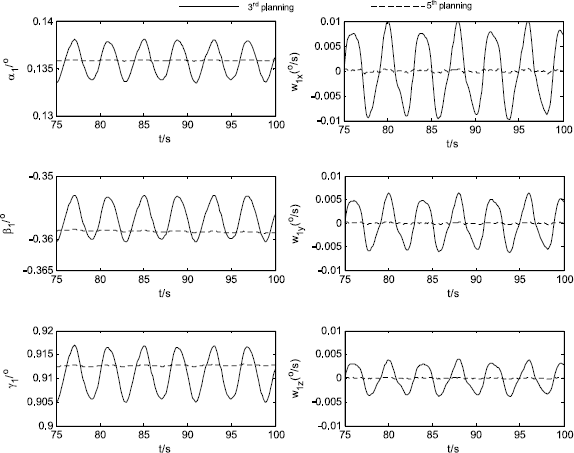

  

  The attitude motion of the robot base resulting from the residual vibration

7 Conclusion

The spacecraft to be launched to space will increase significantly in scale to satisfy more application requirements. Large flexible components such as antenna reflectors and solar paddles should be inevitably mounted onto the spacecraft. To serve such a target, it is required the space robot, which generally has flexible solar wings, to approach, capture, and manipulate it. In this paper, we derived the dynamical equations, developed a closed-loop simulation system, and analyzed the structure vibration of typical applications. Some useful results are obtained as follows:

• (1) For a given path, shorter movement time (larger speed and acceleration) results in greater structure vibration. The vibration amplitude will decrease largely when increasing the movement time. However, too long of time will reduce the efficiency of performing the on-orbital tasks. Therefore, the movement time can be optimized to minimize the vibration under other constraints.

• (2) Good planning algorithm can play a significant role in reducing vibration. For example, the 3rd polynomial algorithm generates non-zeros initial and final accelerations. Thereafter, the acceleration mutation causes larger vibration at the beginning and the end time (i.e., residual vibration). In contrast, the 5th polynomial settles this problem well. However, a single polynomial planning cannot guarantee minimum vibration during the whole movement, especially for complex path planning requirement.

• (3) Although the planned trajectory is optimized by suppressing the vibrations, it is not still assured that the practical movement is reduced, since the planned motion is only an input of the controller. The drive torques generated by the controller will affect the vibration largely. Therefore, it is very important to design advanced control laws to suppress the structure vibration. The dynamics analysis results is very helpful to determine the parameters for the control laws, such as input/command shaping, adaptive feedback/feedforward, artificial neural networks, etc. The planning and control functions should not be considered separately. They should be designed as a whole means to handle the vibration reducing problems.

• (4) The modeling, simulation, and verification method addressed in this paper is very useful for the study of other complex dynamic systems. The derived dynamics equations are written in a recursive form and are resolved by an efficient numerical integration method—Gill method. It is very convenient to program the dynamics calculation code using C language, and then encapsulate it as a Simulink block, which is directly used in Matlab/Simulink environment. Combining the powerful control, display, and other toolboxes, different algorithms for trajectory planning and control can be verified. Similar study on other dynamic system can follow this concept.

Further theory analysis and dynamics simulation show that the relationship between the direction of rigid movement and that of flexible vibration also determines the vibration level. In fact, this angle reflects the coupling effect between the rigid movement and the flexible vibration. The smaller the angle (≤90^o) between the rigid acceleration vector and the vibration direction, the greater vibration of the flexible structure is. When it attains 90^o, almost no vibration corresponding to a certain modal shape occurs. In the future, we will give the details of some application examples.

References

Long, A.M., Richards, M.G., Hastings, D.E.: On-orbit servicing: a new value proposition for satellite design and operation. J. Spacecr. Rockets 44(4), 964–976 (2007)
Joppin, C., Hastings, D.E.: On-orbit upgrade and repair: the Hubble space telescope example. J. Spacecr. Rockets 43(3), 614–625 (2006)
Ellery, A., Kreisel, J., Sommer, B.: The case for robotic on-orbit servicing of spacecraft: spacecraft reliability is a myth. Acta Astronaut. 63(5–6), 632–648 (2008)
Liu, X., Baoyin, H., Ma, X.: Optimal path planning of redundant free-floating revolute-jointed space manipulators with seven links. Multibody Syst. Dyn. 29(1), 41–56 (2013)
Yoshida, K.: Engineering test satellite VII flight experiments for space robot dynamics and control: theories on laboratory test beds ten years ago, now in orbit. Int. J. Robot. Res. 22(5), 321–335 (2003)
Friend, R.B.: Orbital express program summary and mission overview. In: Proceedings of SPIE, Sensors and Systems for Space Applications II, pp. 695801–695803 (2008)
Ioannis Rekleitis, E.M.G.R.: Autonomous capture of a tumbling satellite. J. Field Robot. 24(4), 275–296 (2007). Special Issue on Space Robotics
Yoshida, K., Umetani, Y.: Control of space manipulators with generalized Jacobian matrix. In: Xu, Y.S., Kanade, T. (eds.) Space Robotics: Dynamics and Control, pp. 165–204. Kluwer Academic, Norwell (1993)
Yoshida, K., Nakanishi, H., Ueno, H.: Dynamics, control and impedance matching for robotic capture of a non-cooperative satellite. Adv. Robot. 18(2), 175–198 (2004)
Yoshida, K., Dimitrov, D., Nakanishi, H.: On the capture of tumbling satellite by a space robot. In: Proceedings of the IEEE/RSJ International Conference on Intelligent Robots and System, Beijing, China, pp. 4127–4132 (2006)
Papadopoulos, E., Moosavian, S.A.A.: Dynamics and control of multi-arm space robots during chase and capture operations. In: Proceedings of IEEE International Conference on Intelligent Robots and Systems, Munich, Germany, pp. 1554–1561 (1994)
Nagamatsu, H., Kubota, T., Nakatani, I.: Autonomous retrieval of a tumbling satellite based on predictive trajectory. In: Proceedings of International Conference on Robotics and Automation, Albuquerque, New Mexico, pp. 3074–3079 (1997)
McCourt, R.A., Silva, C.W.: Autonomous robotic capture of a satellite using constrained predictive control. IEEE/ASME Trans. Mechatron. 11(6), 699–708 (2006)
Xu, W.F., Liang, B., Li, C., Liu, Y., Xu, Y.S.: Autonomous rendezvous and robotic capturing of non-cooperative target in space. Robotica 28(5), 705–718 (2010)
Aghili, F.: A prediction and motion-planning scheme for visually guided robotic capturing of free-floating tumbling objects with uncertain dynamics. IEEE Trans. Robot. 28(3), 634–649 (2012)
Xu, Y., Shum, H.: Dynamic control and coupling of a free-flying space robot system. J. Robot. Syst. 11(7), 573–589 (1994)
Dwivedy, S.K., Eberhard, P.: Dynamics analysis of flexible manipulators, a literature review. Mech. Mach. Theory 41(7), 749–777 (2006)
Ma, O., Buhariwala, K., Neil, R., Maclean, J., Carr, R.: MDSF—a generic development and simulation facility for flexible, complex robotic systems. Robotica 15(1), 49–62 (1997)
Talebi, H.A., Patel, R.V., Asmer, H.: Neural network based dynamics modeling of flexible-link manipulators with application to the SSRMS. J. Robot. Syst. 17(7), 385–401 (2000)
Mohan, A., Saha, S.K.: A recursive, numerically stable, and efficient simulation algorithm for serial robots with flexible links. Multibody Syst. Dyn. 21(1), 1–35 (2009)
Sabatini, M., Gasbarri, P., Monti, R., Palmerini, G.B.: Vibration control of a flexible space manipulator during on orbit operations. Acta Astronaut. 73(4–5), 109–121 (2012)
Masoudi, R., Mahzoon, M.: Maneuvering and vibrations control of a free-floating space robot with flexible arms. J. Dyn. Syst. Meas. Control 133(5), 51001–51008 (2011)
Zarafshan, P., Moosavian, S.A.A.: Control of a space robot with flexible members. In: Proceedings of IEEE International Conference on Robotics and Automation, Shanghai, China, pp. 2211–2216 (2011)
Zarafshan, P., Moosavian, S.A.A.: Manipulation control of a space robot with flexible solar panels. In: Proceedings of IEEE/ASME International Conference on Advanced Intelligent Mechatronics, Montréal, Canada, pp. 1099–1104 (2010)
Boning, P., Dubowsky, S.: Coordinated control of space robot teams for the on-orbit construction of large flexible space structures. Adv. Robot. 24(3), 303–323 (2010)
Ono, M., Boning, P., Nohara, T., Dubowsky, S.: Experimental validation of a fuel-efficient robotic maneuver control algorithm for very large flexible space structures. In: Proceedings of IEEE International Conference on Robotics and Automation, Pasadena, CA, USA, pp. 608–613 (2008)
Nagashio, T., Kida, T., Ohtani, T., Hamada, Y.: Design and implementation of robust symmetric attitude controller for ETS-VIII spacecraft. Control Eng. Pract. 18(12), 1440–1451 (2010)
Sylla, M., Asseke, B.: Dynamics of a rotating flexible and symmetric spacecraft using impedance matrix in terms of the flexible appendages cantilever modes. Multibody Syst. Dyn. 19(4), 345–364 (2008)
Zhou, Z., Li, F., Li, Z., Zhang, B.: Development of DFH-4, the third generation of China GEO platform. In: Proceedings of the 57th International Astronautical Congress, Spain, pp. 1–8 (2006)
Xu, W.F., Liang, B., Li, B., Xu, Y.S.: A universal on-orbit servicing system used in the geostationary orbit. Adv. Space Res. 48(1), 95–119 (2011)
Nenchev, D.N., Yoshida, K.: Impact analysis and post-impact motion control issues of a free-floating space robot subject to a force impulse. IEEE Trans. Robot. Autom. 15(3), 548–557 (1999)
Wittenburg, J.: Dynamics of Systems of Rigid Bodies. Teubner, Stuttgart (1977)
Bae, D.S., Haug, E.J.: A recursive formulation for constrained mechanical system dynamics. Part I. Open loop systems. Mech. Struct. Mach. 15(3), 359–382 (1987)
Kim, S.S., Haug, E.J.: A recursive formulation for flexible multibody dynamics. Part I. Open-loop systems. Comput. Methods Appl. Mech. Eng. 71, 293–314 (1988)
Haug, E.J., McCullough, M.: A variational-vector calculus approach to machine dynamics. J. Mech. Transm. Autom. Des. 108(1), 25–30 (1986)
Oliveira, S.C.: Evaluation of effectiveness factor of immobilized enzymes using Runge-Kutta-Gill method: how to solve mathematical undetermination at particle center point? Bioprocess Biosyst. Eng. 20(2), 185–187 (1999)
Xu, W.F., Li, C.L., Liang, B., Xu, Y.S., Liu, Y., Qiang, W.Y.: Target berthing and base reorientation of free-floating space robotic system after capturing. Acta Astronaut. 2–3(64), 109–126 (2009)
Acknowledgements
This work is partly supported by National Natural Science Foundation of China (61175098), Aerospace Science and Technology Innovation Fund (CASC201102), and RFD 2012/2013 at CUHK-Smart China Centre for Research on Robotic and Smart-city.
Author information
Authors and Affiliations
Corresponding author
Rights and permissions
About this article
Cite this article
Xu, W., Meng, D., Chen, Y. et al. Dynamics modeling and analysis of a flexible-base space robot for capturing large flexible spacecraft. Multibody Syst Dyn 32, 357–401 (2014). https://doi.org/10.1007/s11044-013-9389-0
Received:
Accepted:
Published:
Issue Date:
DOI: https://doi.org/10.1007/s11044-013-9389-0