
Abstract
Perceptually salient regions of stereoscopic images significantly affect visual comfort (VC). In this paper, we propose a new objective approach for predicting VC of stereoscopic images according to visual saliency. The proposed approach includes two stages. The first stage involves the extraction of foreground saliency and depth contrast from a disparity map to generate a depth saliency map, which in turn is combined with 2D saliency to obtain a stereoscopic visual saliency map. The second stage involves the extraction of saliency-weighted VC features, and feeding them into a prediction metric to produce VC scores of the stereoscopic images. We demonstrate the effectiveness of the proposed approach compared with the conventional prediction methods on the IVY Lab database, with performance gain ranging from 0.016 to 0.198 in terms of correlation coefficients.
1 Introduction
Stereoscopic three-dimensional (S3D) visualization can provide a viewer an illusion of depth perception, and is the latest step in the evolution of image/video formats. However, when people watch stereoscopic images on current stereoscopic displays, some normal neural function may be disturbed by accommodation-vergence mismatches between the left and right eyes, causing visual discomfort to observers [25]. Over the last two decades, extensive studies have been conducted regarding the health and safety aspects of visual discomfort caused by unnatural stereoscopic images [12, 15, 23, 26, 36]. Several key factors resulting in visual discomfort have been identified, including excessive horizontal disparity [15, 26], fast changes in disparity [23], mismatches between the left and right images of stereo pairs [12], and excessive luminance and chrominance differences between the left and right images [36]. These visual discomforts can result in eyestrain, nausea, and headache. Therefore, it is desirable and of great importance in developing effective and automatic visual comfort (VC) prediction models for appropriate 3D multimedia production.
Recently, biologically plausible computational schemes have been proposed to measure the VC/visual discomfort of stereo images [5, 17–20, 25, 26, 29]. Park et al. [25] investigated the accommodation- vergence conflict and developed the 3D accommodation-vergence mismatch predictor. They then proposed a 3D visual discomfort predictor to predict stereoscopic visual discomfort [26]. Sohn et al. [29] proposed two object-dependent disparity features (i.e., relative disparity and object thickness features) to predict visual discomfort of stereoscopic images. Jung et al. [17] used visually important regions to automatically assess visual discomfort. Choi et al. [5] proposed the visual fatigue evaluation method that considers spatial complexity, temporal complexity, and depth position. Lambooij et al. [20] assessed 3D VC according to the effect of screen disparity offset and range. Kim et al. [19] developed a visual fatigue predictor for stereo images by measuring excessive horizontal and vertical disparities caused by stereoscopic impairments.
However, the human visual system has a remarkable capability of selectively focusing on visually salient areas among overwhelming information from the surrounding environment [32, 33]. The more salient a region is, the more important it is for overall VC production. Consequently, it is necessary to explore the stereo visual saliency for predicting stereo VC. We therefore propose a VC prediction approach based on stereo visual saliency for stereoscopic images. The algorithm can be partitioned into two blocks, stereo visual saliency detection and VC prediction. Our work differs in several aspects from the prior work.
First, we use a regional contrast-based saliency extraction method to compute the depth (disparity) saliency map, in a manner similar to that described in [22]. The previous saliency extraction method for a disparity map involved the assignment of disparity values close to the maximum disparity value for high depth saliency values, while assigning disparity values close to the minimum disparity for low depth saliency values [17]. But the closer objects are not always salient. For example, the ground floor in an image has a wide range of disparity values but the ground is not salient. Based on the observation that the disparity change between an object and its background tends to be abrupt and the change in the ground tends to be smooth, we first compute the local disparity difference along each row and use it to modulate the original disparity map. The local disparity difference modulation can degrade ground saliency. Then, the regional contrast-based saliency detection method is used to extract a salient object from the modulated depth map.
Second, considering that the 3D visual discomfort caused by vergence-accommodation conflict affects visual attention, we linearly combine depth and 2D saliency maps by incorporating disparity comfort. Furthermore, we extract the depth contrast from the disparity map as an important saliency cue, because it directs the viewer’s attention in the viewing of 3D images.
Third, in the VC prediction module, we extract not only the disparity magnitude and disparity gradient but also luminance and chrominance differences from the stereoscopic pairs as significant perceptual features, considering that such excessive differences can result in binocular vision physiological abnormalities [1].
The remainder of the paper is organized as follows. In Section 2, we address the issue of 3D saliency for stereoscopic images. The depth saliency computation and 2D saliency estimation are described in Section 2.1. In addition, a pooling strategy applied on the two saliency maps is introduced in Section 2.2, followed by salient object extraction in Section 2.3. In Section 3.1, we first show the extraction of the disparity magnitude, disparity gradient, and luminance and chrominance differences from the stereoscopic pairs as significant VC features, and then combine these features with stereoscopic saliency maps. Section 3.2 shows our construction of a VC predictor for stereoscopic images based on the extracted VC indices, with the optimized parameters, through support vector regression. Extensive experiments and performance comparisons are performed in Section 4. Finally, conclusions are drawn in Section 5.
2 Stereoscopic image saliency computation
Saliency detection for S3D image/video is a topic of high interest in computer vision studies, a good survey can be found in [2]. Basically, the stereoscopic saliency shall include the 2D texture saliency and depth saliency. Therefore, we develop a stereoscopic saliency model in this work, as shown in Fig. 1, and it consists of three major parts: 1) computation of depth and 2D image saliencies; 2) fusion of depth and 2D saliency maps; and 3) salient object extraction. Details of the three parts of our saliency model are presented in the following sections 2.1 to 2.3.

The computation procedure of stereoscopic saliency model
2.1 Depth saliency computation
Depth information in a stereoscopic image represents the distance between objects and observers [35]. Psychological studies indicate that people’s capability to cognize and identify objects depends heavily on effective utilization of depth information, and there are deep relations between visual attention and depth information [7]. Therefore, depth saliency is an important factor for stereoscopic saliency and VC prediction.
Instead of directly assigning disparity values close to the maximum (minimum) disparity value for high (low) depth saliency values as used in most depth saliency computation algorithms, we develop a depth saliency computation method according to depth region contrast and depth edge as follows.
-
1)
Acquire Disparity Map: In our depth saliency experiments, the disparity maps are distinguished into two groups: those with low-quality disparity maps (e.g., Kendo and Lovebird) are estimated using the depth-estimation reference software [30] and those with higher quality disparity maps (Ballet and Breakdancers; the second and third columns in Fig. 2) are obtained using a laser range camera.
Fig. 2 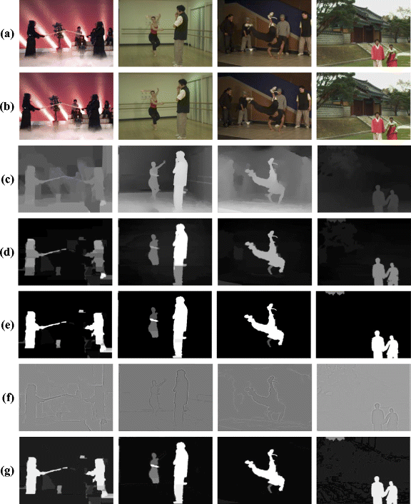
Depth saliency map estimation. a Left-view image. b Right-view image. c Disparity map. d Preprocessed disparity map. e Foreground saliency map. f Depth edge contrast map. g Depth saliency map
-
2)
Compute Depth Salient Object: In general, human eyes tend to focus on foreground objects than background objects [21], indicating that the objects closer to the viewer are more salient than those farther away. However, closer objects are not always salient. For example, in the second column of Fig. 2, although the ground floor with high disparity values is closer to the viewer, it is not salient. By deriving inspiration from [22], we first calculate the local disparity difference along each row, and use it to modulate the original disparity map D as

where p is a pixel in the disparity map, d ′ p and d p are respectively the modulated and original disparity values of pixel p, and \( {\overline{d}}_r \) denotes the average disparity values of the row that contains d p . The disparity values at the ground floor are then reduced (Fig. 2d).
Next, a region contrast-based salient detection algorithm [4] is extended for depth saliency analysis. This approach mainly consists of two steps: the first step is to segment the input image (modulated disparity map D′) into regions by using the graph-based image-segmentation method [8]; the second step is to compute the saliency value of a region R i by measuring its disparity contrast with that of all the other regions in D′,
where S(R i ) is the saliency for region R i , n k is the number of pixels in region R k , and d ′ R (R i , R k ) is the disparity contrast between R i and R k :
where d′(p, q) is the disparity difference between pixels p and q, defined as |d ′ p − d ′ q |, ω(p, q) is a weight computed using the spatial distance between p and q as ω(p, q) = \( {e}^{-{{\left\Vert p-q\right\Vert}_2}^2/{\sigma}^2} \), where σ 2 is a control parameter with default value 0.4, and the image coordinates are normalized to [0, 1].
Finally, according to the observation that the object popping from the screen tends to be salient, we mapped the saliency values S R (x, y) obtained by (2) with
where S ′ R (x, y) is the mapped values at pixel position (x, y), S max and S min are respectively the maximal and minimal saliency values. Figure 2e shows the depth saliency-computation results obtained using (4).
However, simply considering the distance between the object and observer would disregard other useful information of stereoscopic images, such as depth edges and profile details, which are equally important for perception of depth saliency [28, 32]. Among various depth features and their combinations, we choose depth contrast as the main indicator for complexity-performance trade-off. This is because depth contrast is a dominant feature and an effective indicator in depth perception [6]. Figure 3 illustrates the relationship between depth contrast and saliency according to a subjective experiment [32]. Increase in the absolute value of depth increases the fixation probability \( P\left(C=1\Big|{\overline{f}}_{contrast}\right) \).

The relationship between depth values and \( P\left(C=1\Big|{\overline{f}}_{contrast}\right) \). The y-coordinate \( P\left(C=1\Big|{\overline{f}}_{contrast}\right) \) denotes the probability of fixation, and a higher \( P\left(C=1\Big|{\overline{f}}_{contrast}\right) \) value yields a larger possibility of fixation, where C is a binary random variable denoting whether a point is focused upon, and the random variable vector \( {\overline{f}}_{contrast} \) denotes the depth contrast observed from this point
Therefore, the DoG filter is employed to extract the depth edge contrast from the disparity map since it can eliminate anomalous noises of high-frequency signal. The DoG filter is defined as:
where (x, y) is the pixel position, and σ and K are used to control the filter scale and center-surround ratio, respectively. In our experiment, we set σ = 32 and K = 1.6 (approximate to the Laplacian of the Gaussian transform), as commonly used in a previous study [34]. Figure 2f shows the generated depth edge contrast map S E , the edges and profile details of objects are well sharpened as desired. Higher contrast values indicate a larger distance between objects and background, and a higher probability is depth-salient.
Finally, we obtain the depth saliency map (S dep ) by pooling the foreground saliency map(S ' R ) and depth edge contrast map (S E ) as follows:
where w r and w e are the weights of the foreground and contrast saliency maps, w r and w e are set as 0.5. Figure 2 illustrates the depth-saliency computation process. Figure 2g illustrates the final combined depth saliency map.
In addition, the 2D image saliency map S img is computed using the Graph-Based Visual Saliency (GBVS) method [13]. GBVS is one of the classic bottom-up visual saliency models and shows a remarkable consistency with attention deployment of human subjects. Figure 4c shows the computation results of the 2D saliency estimation.

Examples of stereoscopic visual-importance-map estimation. a Left-view image. b Right-view image. c 2D saliency map. d Depth saliency map. e Stereoscopic saliency map. f Salient objects segmentation
2.2 Procurement of stereoscopic saliency map
Human visual perception studies have shown that stereoscopic images with excessive protruding objects or excessive disparity [15] and those which affect the visual attention of observers may cause discomfort to viewers. In other words, if someone feels discomfort for some particular regions, he/she will not gaze at those regions. Hence, we linearly combined the two saliency maps through a weighted sum and meanwhile considered the effect of visual discomfort. The final stereoscopic visual saliency is expressed as
where S 3D(x, y), S img(x, y), and S dep(x, y) are the 3D image, 2D image, and depth-saliency values at pixel position (x, y) in S 3D , S img , and S dep , respectively. γ is a weight with default value 0.5 , and λ is the VC factor at position (x, y):
where T neg and T pos are the lower and upper bound values of the stereoscopic comfort zone, and are predetermined manually or statistically. Figure 4e shows the fusion results by using (7).
2.3 Salient object segmentation
In salient regions, salient objects attract the human eyes more than other objects. To extract a salient object, we calculate the gray histogram of the visual saliency map S 3D , and select the appropriate threshold T to extract the salient object if the S3D(x, y) is larger than the threshold T. The salient objects are obtained by
where S obj (x, y) is a two-valued function employed to extract salient objects, and T is the adaptive threshold value that is determined by Otsu’s algorithm [24]. If the pixel values in S 3D are larger than T, they would become 1, which corresponds to the value of a salient object; otherwise, the pixel values correspond to the value of a nonsalient object. Figure 4f illustrates salient object extraction. As shown in Fig. 4, our method can successfully predict a salient object by considering both depth edge contrast and disparity magnitude information.
To verify the effectiveness of our saliency model, we compared it with five state-of-the-art models proposed by Zhang et al. [34], Guo et al. [11], Hou et al. [14], Harel et al. [13], and Jung et al. [17]. Figure 5 provides the saliency results of these saliency models. Figure 5b shows that Zhang’s model can detect the object outline clearly but may fail to appropriately detect salient regions, and has holes inside of the detected objects. The phase spectrum of quaternion Fourier transform (PQFT) model [11] can preserve the edges of objects but important objects may be missing from salient regions [Fig. 5c]; the spectral residual (SR) method [14] is faster but its result is imperfect [Fig. 5d]; the GBVS [13] predicts that human fixations are more reliable than the aforementioned three methods [Fig. 5e]. Therefore, our model employs GBVS to estimate 2D saliency. In Fig. 5f, Jung’s model obtains a depth saliency map through linear disparity mapping. However, it has a unique problem: objects closer to the viewer are not always highly salient. We can observe that, for the saliency results of Ballet and Breakdancers (the bottom two rows) that obtained via Jung’s model, the floor regions are regarded as salient regions, which is inaccurate and inconsistent to human vision. This is not a region that people would typically gaze at. In contrast, as shown in Fig. 5g, our model can successfully identify the salient-object region of stereoscopic images, especially for the floor regions of Ballet and Breakdancers sequences. This is because of the consideration of both disparity change and depth contrast information and the combination of the two saliency maps using a weighted sum in which the weights are affected by visual discomfort.

The results of saliency detection of various methods. a Original left images. b Zhang’s model. c PQFT model. d SR model. e GBVS model. f Jung’s model. g Proposed model
3 Stereoscopic image VC prediction
3.1 Perceptual features extraction
Previous studies reported that disparity magnitude and disparity gradient are two key parameters for quantifying the visual comfort of stereoscopic images [25, 29]. When the disparity magnitude increases, mismatches of accommodation-vergence become much more severe, which result in visual discomfort. On the other hand, the disparity gradient specifies the difference of disparities between adjacent objects. As the disparity gradient increases, the ability of binocular fusion decreases. Furthermore, literature [36] indicates that the excessive luminance and chrominance difference between the left and right images of stereo pairs may also cause visual discomfort or fatigue.
Hence, in this subsection, we first extract disparity magnitude d(x, y), disparity gradient ∇d(x, y), luminance difference Δv(x, y) and chrominance difference Δh(x, y) from stereo image pairs as the significant perceptual features of VC, and then compute saliency-weighted VC features X = [α 1, α 2, α 3, α 4] as
where M and N are the width and height of the picture, W is a normalization factor defined as
where S obj(x, y) is the binary value at pixel (x, y) in the salient object map S obj . The disparity gradient value at a pixel (x, y) is defined by:
The luminance difference Δv(x, y) and chrominance difference Δh(x, y) are calculated in HSV (Hue, Saturation, Value) color space for its better fidelity to the mechanism regarding how human eyes perceive color [27]. The absolute values of Δv(x, y) and Δh(x, y) at a pixel position (x, y) can be calculated as:
where v L (x, y) and v R (x, y) (h L (x, y) and h R (x, y)) denote the luminance (chrominance) values in the left image and right image, respectively. Note that the color images are generally described in RGB color space, the convert equations for the RGB values into the HSV values can be referenced in the previous work [9]. The range of hue in this context is normalized into [0, 1].
3.2 Visual comfort objective evaluation
Based on the saliency-weighed VC feature vector X of a stereo image, its VC score is calculated by a prediction metric f(X), i.e. VC = f(X). Here, we use ε − SVR model [31] to construct the f(X), which is modeled as
where α and α ∗ are the Lagrange multipliers, b is a bias. Following [31], the kernel function K(X i , X) that performs non-linear transform is defined as:
where γ is the variance of the kernel function. To implement the SVR, the LibSVM package [3] is used, where the parameters are determined by cross-validation during the training process. The penalty parameter C is employed to control the complexity of the prediction function. Here, we set ε = 0.1, C = 64, and γ = 1 as a result of the exhaustive grid search.
4 Experimental results
4.1 Dataset
A publicly available stereoscopic image database, provided by the IVY Lab [16], was used for experiments to verify the effectiveness of our proposed VC prediction approach. The IVY Lab database was captured by a 3D digital camera (Fujifilm FinePix 3D W3®) with a spatial resolution of 1920 × 1080 pixels. It consists of 120 stereo images, along with associated Mean Opinion Score (MOS). To consider the diversity of disparity structures, the 120 stereo images were divided into 62 indoor and 58 outdoor scenes, which contain various types of objects with diverse shapes and depths. Furthermore, each stereo image was assessed by the single stimulus method of ITU-R BT.500-11 with a five-grade scale (1: extremely uncomfortable; 2: uncomfortable; 3: middle comfortable; 4: comfortable; 5: very comfortable).
4.2 Performance assessment
In our experiment, 300-times 10-fold cross-validation [19] was employed to assess the performance of the proposed VC prediction approach. We randomly partitioned the stereoscopic image sample sets into 10 subsets, 9 of all were used as training set, and the remaining one was retained as the validation set for testing the model. In order to avoid influences of some nonlinear factors which come from the subjective evaluation, we employ five-parameters Logistic function [10] to nonlinear fit the predicted comfort metric f(X), and the final visual comfort prediction scores are given by:
where parameters b 1 , b 2 , b 3 , b 4 , and b 5 are determined by using nonlinear optimization (b 1 = 0.474, b 2 = 102.39, b 3 = 2.618, b 4 = 0.853 and b 5 = 0.343).
The four commonly used performance metrics: 1) Pearson Linear Correlation Coefficient (PLCC), 2) Kendall Rank-Order Correlation Coefficient (KROCC), 3) Mean Absolute Error (MAE) and 4) Root Mean Square Error (RMSE) between the subjective MOS scores and the fitted prediction scores, are utilized to measure quantitative correlation between prediction results and subjective comfort. Values of PLCC and KROCC approach to 1 mean high correlation with MOS. Conversely, the predicted results are more accurately if the values of MSE and RMSE are smaller. We compared our method with the other four popular VC prediction methods: Jung’s method [17], Choi’s method [5], Lambooij’s method [20] and Kim’s method [19]. We implemented these methods and adjusted the parameters for each method for a fair comparison. For Choi’s method, the visual fatigue factors caused by temporal complexity and scene movement were removed. Furthermore, in order to examine the effects of different features on visual comfort, we also took various combinations of visual perceptual features (X = [α 1, α 2], or X = [α 1, α 2, α 3], or X = [α 1, α 2, α 4]), and conducted a comparison between different combinations.
4.3 Experimental results and analyses
Tables 1 and 2 tabulate the comparison results of different methods and different perceptual feature combinations. From the tables, we can see that our method outperforms Jung’s, Choi’s, Lambooij’s and Kim’s methods with 0.016, 0.193, 0.102 and 0.051 gains in PLCC, 0.014, 0.198, 0.108 and 0.047 gains in KROCC, 0.03, 0.199, 0.095 and 0.055 decreases in MAE, and 0.024, 0.198, 0.095 and 0.068 decreases in RSME, respectively. Thus, PLCC and KROCC of our proposed method are 0.865 and 0.675 respectively, which are highest values among the benchmarks. Meanwhile, the MAE and RMSE of the proposed algorithm are 0.322 and 0.416, which are the lowest values among the benchmarks. Overall, the proposed approach achieves the best consistency in predicting the VC.
Moreover, we investigate the contributions of adopting different features. As tabulated in Tables 1 and 2, the saliency-weighted disparity magnitude α 1 and disparity gradient α 2 have greater impact on visual comfort, while saliency-weighted luminance difference α 3 and color difference α 4 have less impact, especially color difference. This is because small color differences are corrected by the irises of the eyes. Our proposed method which used all of the extracted features (X = [α 1, α 2, α 3, α 4]) has the best performance. This means that, based on the extraction of disparity magnitude, disparity gradient, luminance difference and chrominance difference of the stereo image pairs, the proposed objective VC prediction method are highly consistent with human visual system, and successfully predicted the visual comfort scores of stereo images.
Figure 6 shows the MOS results of the predictive visual comfort for stereoscopic images by using the proposed method and others, where the blue bar is the subjective evaluation result, the baby-blue bar represent the proposed method, while the other four different color bars stand for the results of Jung [17], Choi [5], Lambooij [20] and Kim [19], respectively. Figure 6a shows VC scores of 15 comfortable stereo images, whose visual comfort scores are all larger than 3.0. We can see that the predicted MOS values of the proposed method are more approach to the subjective MOSs than the other methods. Furthermore, Fig. 6b shows VC scores of 15 uncomfortable stereo images, whose visual comfort scores are all less than 3.0. It can be observed that the predicted results of our method have some deviation, but comparing to the results from the methods proposed in [5, 17, 19, 20], our prediction values are much closer to MOSs and hence can predict visual comfort more effectively. This is because our proposed method not only exploits the depth contrast in depth saliency detection but also uses multiplication to combine depth saliency and 2D saliency, which improves the accuracy of stereoscopic saliency detection. In addition, in order to further improve VC prediction accuracy, our method extracts luminance difference and chrominance difference as additional comfortable perceptual features. Meanwhile, our method reduces unimportant saliency-weighed VC feature impacts by using salient object extraction.

Evaluation results for the visual comfort prediction. a a set of comfortable stereo images (visual comfort score >3.0); b a set of uncomfortable stereo images (visual comfort score <3.0)
In addition, we provide the scatter plot to show the relationship between subjective MOSs and prediction scores using the proposed method. As shown in Fig. 7, the prediction results of the proposed method are concentrated and almost be a good linear relationship with subjective MOS values. Hence, the proposed method is highly correlated with the human visual perception and can effectively predict the VC of stereo images.

Scatter plot between subjective scores and predicted visual comfort scores with the proposed method
5 Conclusions
When analyzing the VC of stereoscopic images, it is important to consider visual attention over a perceived stereoscopic space. Thus, we proposed a VC prediction method based on a visual saliency model in this paper. To detect stereoscopic salient areas, we first extracted foreground salient regions and depth-edge contrast map from the disparity map to obtain the depth saliency map, and combined the depth and 2D saliency maps by using a weighted sum in which the weights were adjusted by visual discomfort. The proposed stereoscopic saliency model successfully preserved the edges and profile salient information of objects. Besides, to improve the prediction accuracy of VC, we extracted the salient object from the stereoscopic saliency map. Next, we extracted some important perceptual features including disparity magnitude, disparity gradient, and luminance and chrominance difference values from stereoscopic image pairs, and combined these features to construct the objective VC predictor. The experimental results indicate that the proposed predictor successfully improves the VC prediction accuracy of stereoscopic images. The VC prediction of stereo images can be applied to various applications such as 3D movie production, stereo image compression, and 3D quality evaluation. In future, we will attempt to extend our model to a 3D video by considering more perception features such as object motion and disparity change of objects of different sizes.
References
Bando T, Lijima A, Yano S (2012) Visual fatigue caused by stereoscopic images and the search for the requirement to prevent them: a review. J Display 33(2):76–83
Banitalebi-Dehkordi A, Nasiopoulos E, Pourazad MT, Nasiopoulos P (2016) Benchmark three- dimensional eye-tracking dataset for visual saliency prediction on stereoscopic three-dimensional video. J Electron Imaging 25(1):1–20
Chang CC, Lin CJ (2006) LIBSVM: a library for support vector machines. ACM Trans Intell Syst Technol 2(3):389–396
Cheng MM, Zhang GX, Mitra NJ et al (2015) Global contrast based salient region detection. IEEE Trans Pattern Anal Mach Intell 37(3):409–416
Choi J, Kim D, Ham B et al (2010) Visual fatigue evaluation and enhancement for 2D-plus-depth video. In: Proc of IEEE international conference on image processing (ICIP), Hongkong, pp 2981–2984
Ee RV, Bank MS, Backus BT (2001) An analysis of binocular slant contrast. Perception 28(9):1121–1145
Ee RV, Erkelens CJ (2001) Anisotropy in Werner’s binocular depth contrast effect. Vis Res 36(15):2253–2262
Felzenszwalb PF, Huttenlocher DP (2004) Efficient graph-based image segmentation. Int J Comput Vis 59(2):167–181
Ghimire D, Lee J (2011) Nonlinear transfer function-based local approach for color image enhancement. IEEE Trans Consum Electron 57(2):858–865
Gottschalk PG, Dunn JR (2005) The five-parameter logistic: a characterization and comparison with the four-parameter logistic. Anal Biochem 343(1):54–65
Guo C, Zhang L (2010) A novel multiresolution spatiotemporal saliency detection model and its applications in image and video compression. IEEE Trans Image Process 19(1):185–188
Haigh SM, Barningham L, Berntsen M et al (2013) Discomfort and the cortical haemodynamic response to coloured gratings. Vis Res 89(5):46–53
Harel J, Koch C, Perona P (2007) Graph-based visual saliency. In: Proc of Advances in Neural Information Processing Systems, pp 545–552
Hou X, Zhang L (2007) Saliency detection: a spectral residual approach. In: Proc of IEEE conference on Computer Vision & Pattern Recognition (CVPR), Minneapolis, USA, pp 1–8
Jiang G, Zhou J, Yu M et al (2015) Binocular vision based objective quality assessment method for stereoscopic images. Multimed Tools Appl 74(18):8197–8218
Jung Y, Sohn h, Lee S, Ro Y (2012) IVY Lab Stereoscopic Image Database [Online]. Available: http://ivylab.kaist.ac.kr/demo/3DVCA/3DVCA.htm
Jung YJ, Sohn, Lee S, Park H (2013) Predicting visual discomfort of stereoscopic images using human attention model. IEEE Trans Circ Syst Video Technol 23(12):2077–2082
Jung C, Wang S (2015) Visual comfort assessment in stereoscopic 3D images using salient object disparity. Electron Lett 51(6):482–484
Kim D, Sohn K (2011) Visual fatigue prediction for stereoscopic image. IEEE Trans Circ Syst Video Technol 21(2):231–236
Lambooij M, IJsseltstejin WA, Heynderickx I (2012) Visual discomfort of 3D-TV: assessment methods and modeling. Displays 32(4):209–218
Lina J, Selim O, Peter K (2009) Influence of disparity on fixation and saccades in free viewing of natural scenes. J Vis 9(1):74–76
Niu Y, Geng Y, Li X, Liu F (2012) Leveraging stereopsis for saliency analysis. In: 25th IEEE Conference on Computer Vision and Pattern Recognition (CVPR 2012), Rhode Island, pp 454–461
Oh C, Ham B, Choi S et al (2015) Visual fatigue relaxation for stereoscopic video via nonlinear disparity remapping. IEEE Trans Broadcast 61(2):142–153
Otsu N (1979) A threshold selection method from gray-scale histograms. IEEE Trans Smc 9:62–66
Park J, Lee S, Bovik AC (2014) 3D visual discomfort prediction: vergence, foveation, and the physiological optics of accommodation. IEEE J Sel Top Sign Process 8(3):415–427
Park J, Oh H, Lee S et al (2015) 3D visual discomfort predictor: analysis of horizontal disparity and neural activity statistics. IEEE Trans Image Process 24(3):1101–1114
Paschos G (2001) Perceptually uniform color spaces for color texture analysis: an empirical evaluation. IEEE Trans Image Process 10(6):932–937
Shao F, Lin W, Gu S et al (2013) Perceptual full-reference quality assessment of stereoscopic images by considering binocular visual characteristics. IEEE Trans Image Process 22(5):1940–1953
Sohn H, Jung YJ, Lee S, Ro YM (2013) Predicting visual discomfort using object size and disparity information in stereoscopic images. IEEE Trans Broadcast 59(1):28–37
Tanimoto M, Fujii T, Suzuki K (2009) Depth estimation reference software (DERS)5.0, ISO/IEC JTCI/SC29/WG11 M16923
Vapnik V (1998) Statistical learning theory. Wiley, New York
Wang J, Dasilva MP, Lecallet P et al (2013) Computational model of stereoscopic 3D visual saliency. IEEE Trans Image Process 22(6):2151–2165
Zhang Y, Jiang G, Yu M (2010) Stereoscopic visual attention model for 3D video. Advances in Multimedia Modeling, Berlin, Germany: Springer-verlag, pp 324–324
Zhang L, Tong M, Marks T et al (2008) SUN: a Bayesian framework for saliency using natural statistics. J Vis 8(7):1–20
Zhaoqing P, Zhang Y, Kwong S (2015) Efficient motion and disparity estimation optimization for low complexity multiview video coding. IEEE Trans Broadcast 61(2):166–176
Zilly F, Kluger J, Kauff P (2011) Production rules for stereo acquisition. Proc IEEE 99(4):590–606
Acknowledgments
The authors are very grateful to the anonymous reviewers whose insightful comments have helped improve the paper. This work was supported in part by Natural Science Foundation of China (NSFC) (Grant Nos. 61401132 and 61471348), in part by Zhejiang Natural Science Funds (Grant No. LY17F020027), in part by Guangdong Natural Science Funds for Distinguished Young Scholar (Grant No. 2016A030306022) and in part by National High Technology Research and Development Program of China (Grant No. 2014AA01A302)
Author information
Authors and Affiliations
Corresponding author
Rights and permissions
About this article

Cite this article
Zhou, Y., He, Y., Zhang, S. et al. Visual comfort prediction for stereoscopic image using stereoscopic visual saliency. Multimed Tools Appl 76, 23499–23516 (2017). https://doi.org/10.1007/s11042-016-4126-3
Received:
Revised:
Accepted:
Published:
Issue Date:
DOI: https://doi.org/10.1007/s11042-016-4126-3