Automatic moving object segmentation methods under varying illumination conditions for video data: comparative study, and an improved method

Abstract

In recent past, many moving object segmentation methods under varying lighting changes have been proposed in literature and each of them has their own benefits and limitations. The various methods available in literature for moving object segmentation may be broadly classified into four categories i.e., moving object segmentation methods based on (i) motion information (ii) motion and spatial information (iii) learning (iv) and change detection. The objective of this paper is two-fold i.e., firstly, this paper presents a comprehensive comparative study of various classical as well as state-of-the art methods for moving object segmentation under varying illumination conditions under each of the above mentioned four categories and secondly this paper presents an improved approximation filter based method in complex wavelet domain and its comparison with other methods under four categories mentioned as above. The proposed approach consist of seven steps applied on given video frames which include: wavelet decomposition of frames using Daubechies complex wavelet transform; use of improved approximate median filter on detail co-efficient (LH, HL, HH); use of background modeling on approximate co-efficient (LL sub-band); soft thresholding for noise removal; strong edge detection; inverse wavelet transformation for reconstruction; and finally using closing morphology operator. The qualitative and quantitative comparative study of the various methods under four categories as well as the proposed method is presented for six different datasets. The merits, demerits, and efficacy of each of the methods under consideration have been examined. The extensive experimental comparative analysis on six different challenging benchmark data sets demonstrate that proposed method is performing better to other state-of-the-art moving object segmentation methods and is well capable of dealing with various limitations of existing methods.

1 Introduction

Moving object detection is a crucial part of automatic video surveillance systems and it is useful in robotics, object detection and recognition, indoor/outdoor object classification and many other applications [21, 35]. To design the moving object segmentation algorithm for intelligent video surveillance systems, several major challenges have to be concerned. Toyama et al. [57] have identified the following challenges in moving object segmentation such as (i) lighting changes, shadows and reflections (ii) dynamic backgrounds such as waterfalls or waving trees (iii) Motionless foreground (iv) small movements of non-static objects such as tree branches and bushes blowing in the wind (v) noise image, due to a poor quality image source (vi) movements of objects in the background that leave parts of it different from the background model (ghost regions in the image) (vii) multiple objects moving in the scene both for long and short periods (viii) shadow regions that are projected by foreground objects and are detected as moving objects. Out of all these issues, changing illumination conditions remain a major problem for moving object segmentation in real-life problems. To take into account these problems, many approaches for automatically adapting background model to dynamic scene variations are proposed [11, 15] and these approaches can be classified into two categories [9] such as non-recursive and recursive. A non-recursive approach uses a sliding-window for background estimation. It stores a buffer of the previous L video frames, and estimates the background image based on the temporal variation of each pixel within the buffer. This causes non-recursive approach to have higher memory requirements than recursive techniques. Recursive approach maintains a single background model that is updated with each new video frame. These approaches are generally computationally efficient and have minimal memory requirements.

The major contributions of this paper include: (1) comparative study of various standard moving object segmentation methods which is classified into four categories i.e., moving object segmentation methods based on (i) motion information (ii) motion and spatial information (iii) learning (iv) and change detection (2) proposed an improved approximation filter based approach for moving object segmentation in complex wavelet domain (3) and presented the comparative study of the proposed method with other state-of -the-art algorithms on a set of challenging video sequences (4) analysis of the sensitivity of the most influencing parameters (http://imagelab.ing.unimore.it/visor/video_details.asp?idvideo=113, http://homepages.inf.ed.ac.uk/rbf/CAVIARDATA1/, http://crcv.ucf.edu/data/crowd.php) [64], and a discussion of their effects. (5) and analysis of the computational complexity and memory consumption of the proposed algorithm.

Rest of the paper is organized as follows: Section 2 presents the Review of moving object segmentation methods. Section 3 presents the proposed method. Experimental results are given in Section 4. Finally, conclusion of the work is given in Section 5.

2 Review of moving object segmentation methods

Different kinds of methods exist to solve the problem of moving object segmentation. Good but incomplete reviews on moving object segmentation methods can be found in [45, 48]. As per available literatures moving object segmentation techniques can be broadly classified into four categories [16, 43, 53] namely (i) segmentation of moving object based on motion-information [4, 6, 8, 26, 30, 37, 40, 44, 60], (ii) segmentation of moving object based on motion and spatial information [5, 24, 41, 42, 49, 50, 56, 58, 59, 61], (iii) segmentation of moving object based on learning [12, 13, 17, 27, 34, 38, 39, 46, 55], and (iv) segmentation of moving object based on change detection [2, 3, 7, 10, 20, 22, 23, 25, 28, 31–33, 36, 51]. A review of some of the classical and state-of-the-art methods under each of the categories is presented in following subsections.

2.1 Moving object segmentation methods based on motion-information

The first category of moving object segmentation methods are based on motion-information which depends on motion estimation of moving objects. Some of the prominent methods available in literature are the works due to Bradski [4], Kim et al. [30], Liu et al. [37], Xiaoyan et al. [60], Mahmoodi [40] and Meier and Ngan [44]. Bradski [4] proposed a motion segmentation method using time motion history image (TMHI) for representing motion which is used to segment and measure the motions induced by the object in a video scene. The limitation of the method is that it can only extract the moving objects but not the static one. A more refined application of this algorithm was proposed by Kim et al. [30] which were based on codebook approach where a codebook is formed to represent significant states in the background using quantization and clustering [30]. It solves some of the above mentioned problems existing in [30], such as sudden changes in illumination, but does not consider the problems of ghost regions or shadow detection. To deal with the issues mentioned in [30], Liu et al. [37] have proposed a moving object segmentation method which is based on cumulated difference, object motion and adaptive thresholding. Xiaoyan et al. [60] have proposed a video object segmentation technique on the basis of adaptive change. This method is not able to remove noise from the video frames. Mahmoodi [40] has proposed a shape based active contour method for video segmentation which is based on a piecewise constant approximation of the Mumford shah functional model. This method is slow as it is based on level set framework. Due to lack of spatial information of objects, these algorithms suffer from unwarranted ghost objects, shadows, changing background, clutter, occlusion, and varying lighting conditions. Meier and Ngan [44] have proposed a moving object segmentation which is based on Hausdorff distance. In this method, a background model is created which automatically adapts slowly and rapidly changing parts and matched against subsequent frames using the Hausdorff distance. The limitation of this method is that the boundaries of the extracted objects are not always accurate. In addition to above mentioned methods, in literature some other approaches [6, 8, 26] in the same domain have been proposed but they also suffer from most of the same problems mentioned as above.

Therefore the important features of the methods under the category Moving object segmentation methods based on motion-information can be summarized as follows:

• The motion information based moving object segmentation methods [4, 6, 8, 26, 30, 37, 40, 44, 60] are fast and usually easy to implement.

• Motion information based moving object segmentation methods handle well the background changes but are not robust to sudden illumination changes.

• Furthermore, they are likely to fail if the contrast between the moving objects and the background is low.

2.2 Moving object segmentation methods based on motion and spatial information

The second category of moving object segmentation methods are based on both motion and spatial information. The segmentation of moving objects based on motion and spatial information provide more stable object boundary extraction. Some of the prominent works under this domain are the works due to Mei et al. [42], Mcfarlane and Schofield [41], Remagnino et al. [49], Wren et al. [59], Zivkovic [61], Reza et al. [50], and Ivanov et al. [24]. In paper [42], Mei et al. proposed an automatic segmentation method for moving objects based on the spatial-temporal information of video. In this method, the author utilizes the spatial-temporal information. Spatial segmentation is applied to divide each image into connected areas to find precise object boundaries of moving objects. The limitation of this method is that the boundaries of the extracted objects are not always accurate enough to locate them in different scenes. Mcfarlane and Schofield [41] have proposed an approximation median filter method for segmentation of multiple video objects. This technique has also been used in background modeling for urban traffic monitoring [49]. The major disadvantage of this method is that it needs many frames to learn the new background region revealed by an object that moves away after being stationary for a long time [9] but this method is computationally efficient. Wren et al. [59] have proposed Running Gaussian Average model for moving object segmentation. This model is based on Gaussian probability density function (pdf) where a running average and standard deviation are maintained for each color channel. The drawback of this method lies in its complex nature which makes its processing slow because of the computational overhead involved in updating the mixture models. To deal with the issues mentioned in [59], Zivkovic [61] have proposed a moving object segmentation technique which is combination of temporal and spatial features. This approach automatically adapts the number of Gaussians being used to model for a given pixel. Reza et al. [50] have proposed a moving object segmentation technique, combining temporal and spatial features. This approach takes into account a current frame, ten preceding frames and ten next consecutive frames to segment the moving object. The method detects moving objects independent of their size and speed but there is no provision for reduction of blur and noise from frames, which may lead to inaccurate object segmentation. Ivanov et al. [24] have proposed an improvement over background subtraction method, which is faster than that proposed by [50] and is invariant to runtime change illuminations. In addition to above mentioned methods there are many other works reported in literature [5, 56, 58] under this second category but most of them suffers from the similar types of limitations associated with above mentioned methods.

Therefore the important features of the methods under the category Moving object segmentation methods based on motion- and spatial information can be summarized as follows:

• The motion and spatial information based moving object segmentation methods [5, 24, 41, 42, 49, 50, 56, 58, 59, 61] needs many frames to learn the new background region revealed by an object that moves away after being stationary for a long time [9]

• motion and spatial information based moving object segmentation methods is adaptive to only the small and gradual changes in the background and in case of sudden changes it distorts

• Computational complexity of spatial information based moving object segmentation methods is also very low.

2.3 Moving object segmentation methods based on learning

The Third category of moving object segmentation methods are based on learning which depends on some predefined learning patterns. Some of the prominent methods available in literature are the works due to Oliver et al. [46], Cucchiara et al. [12], Kushwaha et al. [34], Kato et al. [27], Ellis et al. [17], and Stauffer et al. [55]. Oliver et al. [46] proposed a moving object segmentation method which is based on spatial correlations. In this method, author constructs the background using principal component analysis. But it’s suffered the problem of noise and blur. To deal the issue mention in [46], Cucchiara et al. [12] have proposed a moving object segmentation technique which is based on medoid filtering that can lead to color background estimation. The medoid filtering is capable of saving boundaries and existing edges in the frame without any blurring. But the computational complexity to construct the background is high. A more refined application of this algorithm proposed by Kushwaha et al. [34] which is based on construction of basic background model where in the variance and covariance of pixels are computed to construct the model for scene background which is adaptive to the dynamically changing background. The method described in [34] has the capability to relearn the background to adapt background changes. Kato et al. [27] have proposed a segmentation method for monitoring of traffic video based on Hidden Markov Model (HMM). In this method, each pixel or region is classified into three categories: shadow, foreground and background. This method comprises of two phases: learning phase and segmentation phase. Ellis et al. [17] have proposed online segmentation of moving objects in video using online learning. In this approach, motion segmentation is done using semi-supervised appearance learning task wherein supervising labels are autonomously generated by a motion segmentation algorithm but the computational complexity of this algorithm is very high. Stauffer et al. [55] have proposed a tracking method wherein motion segmentation was done using mixture of Gaussians and on-line approximation to update the model. This model has some disadvantages such as background having fast variations cannot be accurately modeled with just a few Gaussians (usually 3 to 5), causing problems for sensitive detection. In addition to above mentioned methods, in literature various other approaches [13, 38, 39] in the same domain have been proposed but they also suffer from most of the same problems mentioned as above.

Therefore the important features of the methods under the category Moving object segmentation methods based on learning information can be summarized as follows:

• Learning based moving object segmentation methods [12, 13, 17, 27, 34, 38, 39, 46, 55] are adaptive to the dynamically changing background

• Computational complexity of Learning based moving object segmentation methods is very high.

• Learning based moving object segmentation methods suffer the problem of shadow regions and the presence of ghosts like appearances.

2.4 Moving object segmentation methods based on change detection

The fourth category of moving object segmentation methods are based on change detection which depends on frame difference of two or more frames. Some of the prominent methods available in literature are the works due to Kim et al. [33], Chien et al. [10], Kim and Hwang [31], Shih et al. [51], Huang et al. [22, 23], Baradarani [2, 3], Hsia et al. [20], Khare et al. [28]. Kim et al. [33] proposed moving object segmentation and automatic object tracking approach for video sequences. In this approach, intra-frame and inter-frame segmentation modules are used for segmentation and tracking. The intra-frame segmentation incorporates user interaction in defining a high level semantic object of interest to be segmented and detects precise object boundary. The inter-frame segmentation involves boundary and region tracking to capture temporal coherence of moving objects with accurate object boundary information. The drawback of this method is that user-interaction is required for separating moving objects from the background in video sequences. To deal with the issues mentioned in [33], Chien et al. [10] proposed moving object Segmentation algorithm using background registration method. The background registration method is used to construct reliable background information from the video sequence. In this approach, a morphological gradient operation is used to filter out the shadow. The major disadvantage of this method is that it adapts only static background and suffers from the problem of ghost objects. Kim and Hwang [31] derive an edge map using change detection method and after removing edge points which belong to the previous frame, the remaining edge map is used to extract the video object plane. This method suffers from the problem of object distortion. To solve this problem, Shih et al. [51] used change detection method in three adjacent frames which easily handles the new appearance of the moving object. Huang et al. [22, 23] proposed an algorithm for moving object segmentation to solve the double-edge problem in the spatial domain using a change detection method with different thresholds in four wavelet sub-bands. Baradarani [2, 3] refined the work of Huang et al. [22, 23] using dual tree complex filter bank in wavelet domain. These methods [2, 3] suffer from the problem of noise disturbances and distortion of moving segmented objects due to change in speed of objects. To concern these issues, Hsia et al. [20] proposed a modified directional lifting-based 9 /7 discrete wavelet transform (MDLDWT) based approach, which is based on the coefficient of lifting-based 9/7 discrete wavelet transform (LDWT). Its advantages of low critical path, fast computational speed and the LL3-band of the MDLDWT is employed solely to reduce the image transform computing cost and remove noise but it cannot handle large dynamic background changes. Khare et al. [28] refine the work of Baradarani [2, 3] and Huang et al. [22, 23] using Daubechies complex wavelet. The method proposed by Khare et al. [28] reduces the noise disturbance and speed change, but it suffers from the problem of dynamic background changes and shadow detection and due to this segmenting coherence occurs [36]. In addition to above mentioned methods, in literature various other approaches [7, 25, 32] in the same domain have been proposed but they also suffer from most of the same problems mentioned as above.

Therefore the important features of the methods under the category Moving object segmentation methods based on change detection [2, 3, 7, 10, 20, 22, 23, 25, 28, 31–33, 36, 51] can be summarized as follows:

• Change detection based moving object segmentation methods [2, 3, 7, 10, 20, 22, 23, 25, 28, 31–33, 36, 51] are adaptive to detect only “significant” changes while rejecting “unimportant” ones.

• Change detection based moving object segmentation methods [2, 3, 7, 10, 20, 22, 23, 25, 28, 31–33, 36, 51] handle noise disturbance and speed change very well,

• Change detection based moving object segmentation methods [2, 3, 7, 10, 20, 22, 23, 25, 28, 31–33, 36, 51] suffer from the problem of either slow speed of moving object or abrupt lighting variation changes.

• The other limitations include shadow regions, detection of only moving objects, and the presence of ghosts like appearances.

The Table 1 presents the summary of various moving object segmentation methods under above mentioned four categories. The brief description of methods, their advantages, limitations, and conclusions of each category are highlighted. For comparative analysis purposes, only few prominent and latest methods in each category are considered which are performing better in their peer groups as reported in literature and demonstrated in results and analysis section.

Table 1 Summary of various moving object segmentation methods

After presenting the literature review of various moving object segmentation methods, discussed as above under each of the four categories, it is observed that the approximate median filter based method under second category i.e., a method based on motion and spatial information is better in comparison to methods presented in other categories also validated through experimental results and analysis presented in Section 4. The approximate median filter contains two steps to segment the object: (i) frame differencing of two consecutive frames (ii) and background modeling step. The brief working of approximation median filter based method for moving object segmentation is given as follows [41, 49]:-

• Step I: Frame Differencing:

  For background subtraction the frame difference FD_n(i,j) is obtained by taken the absolute difference two consecutive frames (n-1) & n. This process can be written as follows:-

  $$ \begin{array}{c}\kern1em For\ every\ pixel\ location\ \left(i,j\right)\ \epsilon\ the\ co- ordinate\ of\ frame\kern1em \\ {}\kern1em {FD}_n\left(i,j\right)=\left|{f}_n\left(i,j\right)-{f}_{n-1}\left(i,j\right)\right|\kern1em \\ {}\kern1em If\kern0.28em {FD}_n\left(i,j\right)<{V}_{thr}\kern1.24em \\ {}\kern1em {FD}_n\left(i,j\right)=0\kern1em \end{array} $$

• Step II: Background Modeling:

  In background modeling step, if the corresponding pixel in the current frame f _n (i, j) is greater in value of previous frame f _n − 1(i, j) then previous frame is incremented by one otherwise previous frame is decreased by one. This process can be written as follows:-

  $$ \begin{array}{l} If\left({f}_n\left(i,j\right)>{f}_{n-1}\left(i,j\right)\right)\\ {}\begin{array}{cc}\hfill \kern0.8em then\kern1.4em \hfill & \hfill {f}_{n-1}\left(i,j\right)={f}_{n-1}\hfill \end{array}\left(i,j\right)+1\\ {}\begin{array}{cc}\hfill \kern0.8em otherwise\hfill & \hfill {f}_{n-1}\left(i,j\right)={f}_{n-1}\left(i,j\right)\hfill \end{array}-1\end{array} $$

  Here, f _n (i, j) is the value of (i, j)^th pixel of n^th frame and f _n − 1(i, j) is the value of (i, j)^th pixel of (n-1)^th frame, V _thr is a threshold value and FD _n (i, j) is the frames difference.

The main limitation of approximate median filter based method is that it does not adapt to the dynamic changes in background due to its weak background modeling steps. Due to this it suffers from the problems of (i) ghost like appearances in moving segmented object (ii) slow adaptation toward a large change in background. (iii) and requirement of many frames to learn the new background region revealed by an object that moves away after being stationary for a long time.

Motivated by these facts, in this paper, we have improved the background modeling step of traditional approximate median filter based method [41, 49] using different major changes such as background registration, background differencing, and background difference mask in complex wavelet domain. These major changes adapt the dynamic background changes and solve the above mentioned three problems in traditional approximate median filter. The effectiveness of the proposed method over traditional approximate median filter is validated through experimental result and analysis presented in section 4.

The main advantage of performing the above mentioned tasks in the complex wavelet domain is that the complex wavelet transform has better noise resilience nature as the lower frequency sub-band of the wavelet transform has the capability of a low-pass filter. The other advantage is that the high frequency sub-bands of complex wavelet transform represent the edge information that provide a strong cue to handle shadow. The proposed method is well capable of dealing with the problems of noise, ghost like appearances, distortion of objects due to the speed of moving objects, dynamic background scenes, varying illumination conditions, shadows, and computational complexity as demonstrated and reported in this paper for several challenging test video sequences.

3 An improved approximation median filter based approach in complex wavelet domain: the proposed method

In this paper, an efficient approach for moving object segmentation under varying illumination conditions is proposed. The proposed method is the modified and extended version of traditional approximation median filter based method for moving object segmentation [41, 49] in complex wavelet domain as discussed in section 2. The proposed method consists of following seven steps as follows and also illustrated in Fig. 1:

Fig. 1

Block diagram of the proposed method

• (i) Complex wavelet decomposition of sequence of frames,

• (ii) Application of approximate median filter on the wavelet coefficients,

• (iii) Application of background modeling,

• (iv) Application of soft thresholding for noise removal,

• (v) Application of canny edge detector to detect strong edges,

• (vi) Application of inverse Daubechies complex wavelet transform,

• (vii) and finally the application of closing morphological operators.

All above steps are iteratively applied until the result does not surpass the set threshold value for object segmentation.

The workings of these steps are given as follows and illustrated in Figs. 1 and 2.

Fig. 2

Sub-block diagram of the proposed approach

• Step 1: Wavelet Decomposition of frames

  In the proposed approach, a 2-D Daubechies complex wavelet transform is applied on current frame and previous frame to get wavelet coefficients in four sub-bands: LL, LH, HL and HH. The generating Daubechies complex wavelet transform is described as follows:

  The basic equation of multi-resolution theory is the scaling equation [14]

  $$ \phi (u)=2{\displaystyle \sum_i{a}_i\phi \left(2u-i\right)} $$

  (1)

  where a_i’s are coefficients, and ϕ(u) is the scaling function. The a_i’scan be real as well as complex valued. Daubechies’s wavelet bases {ψ _j,k (t)} in one-dimension is defined using the above mentioned scaling function ϕ(u) and multi resolution analysis of L₂(ℜ) [14]. The generating wavelet ψ(t) is defined as:

  $$ \psi (t)=2{\displaystyle \sum {\left(-1\right)}^n}\overline{a_{1-n}}\phi \left(2t-n\right) $$

  (2)

  Where ϕ(t) and ψ(t) share same compact support [−L, L + 1].

  Any function f (t) can be decomposed into complex scaling function and mother wavelet as:

  $$ f(t)={\displaystyle \sum_k{C}_k^{jo}{\phi}_{jo,k}}(t)+{\displaystyle \sum_{j=jo}^{j_{\max }-1}{d}_k^j\kern0.28em {\psi}_{j,k}}(t) $$

  (3)

  where, j _o is a given low resolution level, {C ^jo _k } is called approximation coefficient and {d ^j _k } is known as detail coefficient.

  Applying the approximate median filter based method [41, 49] in complex wavelet domain have following advantages (a) it is shift invariant and have a better directional selectivity as compared to real valued wavelet transforms [14] (b) it has perfect reconstruction property (c) it provides true phase information [14], while other complex wavelet transform does not provide true phase information (d) Daubechies complex wavelet transform has no redundancy [14].

• Step 2: Application of improved approximate median filter method on wavelet co-efficient

  In step 2, an approximate median filter based method is applied on detail wavelet coefficients i.e., on sub-bands: LH, HL, and HH. Let Wf _n, d (i, j) (d = {LH, HL, HH}) and Wf _{n − 1, d} (i, j) (d = {LH, HL, HH}) are the wavelet coefficients at location (i, j) of the current frame and previous frame. Instead of assigning a fixed a priori threshold V _th ,d to each frame difference, this paper uses the fast Euler number computation technique [52] to automatically determine V _th ,d from the video frame. The fast Euler numbers algorithm calculates the Euler number for every possible threshold with a single raster of the frame difference image using following equation:

  $$ E\;(i)=\frac{1}{4}\;\left[\left({q}_1(i)-{q}_3\;(i)-2\;{q}_d(i)\right)\right] $$

  (4)

  where q ₁, q ₃, and q _d is the quads (quad is a 2*2 masks of bit cells) contained in the given image.

  The output of the algorithm is an array of Euler numbers: one of each threshold value. The Zero Crossings find out the optimal threshold. Detailed algorithms for the fast Euler number computation method can be found in [52].

  The wavelet domain frame difference WD _n, d (i, j) for respective sub-bands are computed as:

  $$ \begin{array}{l}for\ every\ pixel\ location\ \left(i,\ j\right)\ \epsilon\ the\ co- ordinate\ of\ frame\\ {}{\displaystyle {WD}_{n,\;d}}\left(i,j\right)=\left\{\begin{array}{cc}\hfill 1\hfill & \hfill if\kern0.6em \left|W{f}_{n,\;d}\left(i,j\right)-W{f}_{n-1,\;d}\left(i,j\right)\right|>{V}_{th, d}\hfill \\ {}\hfill 0\hfill & \hfill otherwise\hfill \end{array}\right.\\ {}\kern2.52em \end{array} $$

  (5)

• Step 3: Application of background modeling using LL sub-band

  This step of the proposed method deals with the problems of slow adaptiveness toward a large change in background and requirement of many frames to learn the new background region revealed by an object that moves away after being stationary for a long time as noted in traditional approximate median filter based method [41, 49]. To deal with these issues, here we propose to modify the background modeling approach which uses background registration mask, background difference mask and the frame difference mask to construct the background in LL sub band. The background modeling step is divided in to four major steps as shown in Fig. 3.

  Fig. 3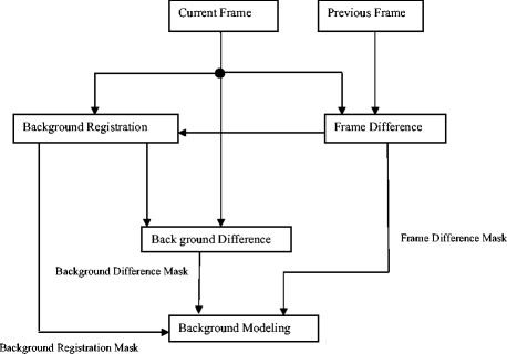

  

  Block diagram of the background modeling in LL sub-band

  The first step calculates the frame difference mask WD _n, LL (i, j) of the LL image which is obtained by thresholding the difference between coefficients in two LL sub-bands as follows:

  $$ {\displaystyle {WD}_{n,\;LL}}\left(i,j\right)=\left\{\begin{array}{ll}1\hfill & if\kern0.6em \left|W{f}_{n,\;LL}\left(i,j\right)-W{f}_{n-1,\;LL}\left(i,j\right)\right|<{V}_{th, WD}\hfill \\ {}0\hfill & otherwise\hfill \end{array}\right. $$

  (6)

  where V _th ,FD is a threshold of WD _n, LL (i, j) determined automatically from the video frame by the fast Euler number computation method as explained in [52]. If WD _n, LL (i, j) = 0, then the difference between two frames is almost the same.

  The second step of background modeling maintains an up-to-date background buffer as well as background registration mask indicating whether the background information of a pixel is available or not. According to the frame difference mask of the past several frames, pixels that are not moving for a long time are considered as reliable background. The reliable background, BR _n, LL (i, j) is defined as

  $$ {\displaystyle {BR}_{n,\;LL}}\left(i,j\right)=\left\{\begin{array}{ll}B{R}_{n-1,\;LL}\left(i,j\right)+1\hfill & if\kern0.48em {\displaystyle {WD}_{n,\;LL}}\left(i,j\right)=0\hfill \\ {}0\hfill & otherwise\hfill \end{array}\right\} $$

  (7)

  The BR _n, LL (i, j) value is accumulated until WD _n, LL (i, j) holds zero value. At any time that WD _n, LL (i, j) is changed from 0 to 1, BR _n, LL (i, j) becomes zero.

  In third step of background modeling, if the value in BR _n, LL (i, j) exceeds a predefined value, denoted by L, then the background difference masks BD _n, LL (i, j) is calculated. It is obtained by taking the difference between the current frame and the background information stored. This background difference mask is the primary information for object shape generation i.e.,

  $$ {\displaystyle {BD}_{n,\;LL}}\left(i,j\right)=\left\{\begin{array}{ll}1\hfill &\;if\kern0.6em \left|B{f}_{n-1,\;LL}\left(i,j\right)-W{f}_{n,\;LL}\left(i,j\right)\right|>{V}_{th, BD}\hfill \\ {}0\hfill & otherwise\hfill \end{array}\right\} $$

  (8)

  where Bf _{n − 1, LL} (i, j) is the pixel value in the current frame that is copied to the corresponding pixel in the BR _n, LL (i, j), and V _th ,BD is a threshold value determined automatically from the video frame by the fast Euler number computation method as explained in [52]. In the case of BR _n, LL (i, j) < L, it is assumed that the background is not constructed, so frame differences mask WD _n, LL (i, j) is used which is calculated in the first step.

  In the fourth step of background modeling, a background model is constructed using the background difference mask, background registration mask and the frame difference mask. The background model generated has some noise regions because of irregular object motion and noise. Also, the boundary region may not be very smooth. The workings of these steps are given as follows and illustrated in Fig. 3.

• Step 4: Application of soft thresholding method for noise removal

  After applying approximate median filter based method and background modeling, the obtained result may have noise. This step deals with the noise reduction from the data obtained in step 2 and step 3. In presence of noise, the equation is expressed as:

  $$ {\displaystyle {WD}_{n,d=\left(LL,LH,HL,HH\right)}}\left(i,j\right)={\displaystyle {W{D}^{*}}_{n,d=\left(LL,LH,HL,HH\right)}}\left(i,j\right)+\eta $$

  (9)

  where WD* _{n,d = (LL,LH,HL,HH)}(i, j) is frame difference without noise, WD _{n,d = (LL,LH,HL,HH)}(i, j) is the original frame difference with noise, and η is the additive noise. The wavelet domain soft thresholding T is applied on wavelet coefficients for noise reduction. The value of soft thresholding parameter T for de-noising is computed as [29]

  $$ T=\frac{1}{2^{j-1}}\left(\frac{\psi }{\xi}\right)\omega $$

  (10)

  where j is wavelet decomposition level and ψ _, ξ and ω are standard deviation, absolute mean and absolute median of wavelet coefficients of a sub-band.

• Step 5: Application of canny edge detector to detect strong edges in wavelet domain

  Canny edge detection method is one of the most useful and popular edge detection methods, because of its low error rate well localized edge points and single edge detection response [54]. In next step, the canny edge detection operator is applied on WD* _{n,d = (LL,LH,HL,HH)}(i, j) to detect the edges of significant difference pixels in all sub-bands as follows:

  $$ D{E}_{n,d=\left(LL,LH,HL,HH\right)}\left(i,j\right)= canny\left({\displaystyle {W{D}^{*}}_{n,d=\left(LL,LH,HL,HH\right)}}\left(i,j\right)\right) $$

  (11)

  where DE _{n,d = (LL,LH,HL,HH)}(i, j) is an edge map of WD* _{n,d = (LL,LH,HL,HH)}(i, j).

• Step 6: Application of inverse Daubechies complex wavelet transform

  After finding edge map DE _{n,d = (LL,LH,HL,HH)}(i, j) in wavelet domain, inverse wavelet transform is applied to get moving object edges in spatial domain i.e., E _n

• Step 7: Application of closing morphological operation to sub-band

  As a result of step 6, the obtained segmented object may include a number of disconnected edges due to non-ideal segmentation of moving object edges. Extractions of object using these disconnected edges may lead to inaccurate object segmentation. Therefore, some morphological operation is needed for post-processing of object edge map to generate connected edges. Here, a binary closing morphological operation is used [54] which gives M(E _n ) i.e., the set of connected edge. In this step, the segmented output is obtained.

4 Experimental results and comparative studies

4.1 Dataset description

In this section, a brief overview of few datasets used for experimentation purpose in this paper are presented.

4.1.1 Pets dataset (http://www.cvg.rdg.ac.uk/PETS2013/a.html)

First video dataset used for experimentation in this paper is the people video sequence which is part of Pets dataset available from (http://www.cvg.rdg.ac.uk/PETS2013/a.html.). This video data contains 2967 frames of frame size 480×272. The main characteristics of this video data are that they are record in outdoor environment wherein multiple objects (Human beings and cars) are present and cases of partial and full occlusions among human beings are also present.

4.1.2 Visor datasets (http://www.openvisor.org/video_details.asp?idvideo=114, http://imagelab.ing.unimore.it/visor_test/video_details.asp?idvideo=194, http://imagelab.ing.unimore.it/visor/video_details.asp?idvideo=113)

The another video data considered for experimentation is the Visor dataset which is the largest publically available and most standard dataset widely used for benchmarking results for segmentation. In this paper, three video data sets from this category are used for experimentation which are Intelligent Room video sequence (http://www.openvisor.org/video_details.asp?idvideo=114) containing 299 frames each of size 320×240, Camera2_070605 video sequence (http://imagelab.ing.unimore.it/visor_test/video_details.asp?idvideo=194) containing 2881 frames each of size 384×288 and HighwayI_raw dataset (http://imagelab.ing.unimore.it/visor/video_details.asp?idvideo=113) containing 439 frames each of size 320×240. Camera2_070605 video sequence dataset is performed at particular angle and is of low-quality and low contrast. Intelligent Room video sequence is recorded in full noisy environment i.e., video quality is low with poor contrast and shadow of object is also present. In highwayI_raw video sequence is recorded in full noisy environment and full and partial occlusion occurs between fast moving cars.

4.1.3 Caviar dataset (http://homepages.inf.ed.ac.uk/rbf/CAVIARDATA1/)

The next video data considered for experimentation is the one step video sequence dataset which is the part of Caviar video dataset available from http://homepages.inf.ed.ac.uk/rbf/CAVIARDATA1/. This video data contains number of video clips, having 1995 frames each of size 480×272, which were recorded acting out the different scenarios of interest. This video is recorded in stationary background situation and multiple human beings are present in the video.

4.1.4 CVCR dataset (Crowdie environment dataset) (http://crcv.ucf.edu/data/crowd.php)

The final data set used for experimentation contains videos of crowds’ density environment. 4917-5_70 is one of the video sequences of CVCR dataset (http://crcv.ucf.edu/data/crowd.php) which contain 1789 frames each of size 480×320. This video was shooted on much more height and in very crowdie environment which contains full occlusions, shadow and noise.

4.2 Performance measures

It is very difficult to compare the segmentation results visually because human visual system can identify and understand scenes with different connected objects effortlessly. Therefore, quantitative performance metrics together with visual results are more appropriate. The performance measures are categorized into various categories for determining the performance of the chosen method or comparing the proposed method with other methods for moving object segmentation. The various categories of performance measures calculate the accuracy of moving object segmentation; measures for noise removal in moving object segmentation; and computational time and memory required in moving object segmentation. The performance measures listed under various categories are defined as follows:

4.2.1 Accuracy of moving object segmentation

The accuracy of moving object segmentation is calculated using following metrics defined as below:

Relative foreground area measure (RFAM) [19]

RFAM gives accurate measurements of the object properties such as area and shape, more specifically the area of the detected and expected foreground. It is calculated between ground-truth frame and segmented frame [19]. The value of RFAM is in the range [0, 1] and if it is 1 then it indicates that the chosen method perfectly segment the moving object. The RFAM is calculated as follows:

$$ RFAM=1-\frac{\left| Area\left({I}_{GTV}\right)-\left. Area\left({I}_{SEGM}\right)\right|\right.}{Area\left({I}_{SEGM}\right)} $$

(12)

where Area(I _GTV ) and Area(I _SEGM ) are area in objects in ground –truth frame and resulting segmented frame, respectively.

Misclassification penalty (MP) [19]

The MP estimated in the segmentation results which are farther from the actual object boundary (ground-truth image) are penalized more than the misclassified pixels which are closer to the actual object boundary [19]. The MP value lies in the range [0, 1]. Zero value of MP means perfect segment the moving object and performance of segmentation methods degrades as the value of MP becomes higher. The MP is defined as follows:

$$ MP=\frac{{\displaystyle {\sum}_{\left(i,j\right)}X\left(i,j\right)\;.\;{\displaystyle {Chem}_{GTV}}\left(i,j\right)}}{{\displaystyle {\sum}_{\left(i,j\right)}{\displaystyle {Chem}_{GTV}}\left(i,j\right)}} $$

(13)

where Chem _GTV denotes the Chamfer distance transform of the boundary of ground-truth object. Indicator X can be computed as

$$ X\left(i,j\right)=\left\{\begin{array}{lll}1,\hfill & if\hfill & {\displaystyle {I}_{GTV}}\left(i,j\right)\ne {\displaystyle {I}_{SEGM}}\left(i,j\right)\hfill \\ {}0\hfill & if\hfill & {\displaystyle {I}_{GTV}}\left(i,j\right)={\displaystyle {I}_{SEGM}}\left(i,j\right)\hfill \end{array}\right\} $$

(14)

where I _GTV (i, j) and I _SEGM (i, j) are ground-truth frame and segmented frame respectively with dimension (i × j) .

Pixel classification based measure (PCM) [19]

The PCM reflects the percentage of background pixels misclassified as foreground pixels and conversely foregrounds pixels misclassified as background pixels [19]. The values of PCM lies in the range [0, 1] with its value 1 indicating perfect moving object segmentation. The PCM is defined as follows:

$$ PCM=1-\frac{Cardi\;\left({\displaystyle {B}_{GTV}}\cap {\displaystyle {F}_{SEGM}}\right)+ Cardi\;\left({\displaystyle {F}_{GTV}}\cap {\displaystyle {B}_{SEGM}}\right)\;}{Cardi\;\left({\displaystyle {B}_{GTV}}\right)+ Cardi\;\left({\displaystyle {F}_{GTV}}\right)\;} $$

(15)

Where B _GTV and F _GTV denote the background and foreground of the ground-truth frame, whereas B _SEGM and F _SEGM denote the background and foreground pixels of the achieved segmented frame ‘∩’ is the logical AND operation. Cardi(.) is the cardinality operator.

Relative position based measure (RPM) [19]

RPM is defined as the centroid shift between ground-truth and segmented object mask. It is normalized by parameter of the ground-truth object [19]. The value of RPM is 1 for perfect moving object segmentation. The RPM is calculated as:

$$ RPM=1-\frac{\left\Vert {\displaystyle {Cent}_{GTV}}-{\displaystyle {Cent}_{SEGM}}\right\Vert }{2\sqrt{\pi}\;.\;\sqrt{{\displaystyle {Area}_{GTV}}}} $$

(16)

where Cent _GTV and Cent _SEGM are centroid of objects in ground-truth frame and achieved segmented frame respectively. Area _GTV is the area of object in ground-truth frame. ||.|| is the Euclidean distance. The centroid of ground truth object can be expressed as

$$ {\displaystyle {Cent}_{GTV}}\;(i)=\frac{{\displaystyle {\sum}_{i,j\in {\displaystyle {X}_{GTV}}}i}}{{\displaystyle {\sum}_{i,j\in {\displaystyle {X}_{GTV}}}1}}\;\mathrm{and}\;{\displaystyle {Cent}_{GTV}}\;(j)=\frac{{\displaystyle {\sum}_{i,j\in {\displaystyle {X}_{GTV}}}j}}{{\displaystyle {\sum}_{i,j\in {\displaystyle {X}_{GTV}}}1}} $$

(17)

4.2.2 Noise removal capacity in moving object segmentation

Here three performance measurement metrics namely Peak Signal-to-Noise Ratio [47], Normalized Absolute Error (NAE) [1], and Normalized Cross Correlation [18] are used for noise. These metric are defined as follows

Peak signal-to-noise ratio (PSNR) [47]

The mean square error (MSE) and the peak signal-to-noise ratio (PSNR) are the two error metrics used to compare image compression quality [47]. Higher value of PSNR means good segmentation (i.e., noise is minimum) while low value of PSNR indicates poor segmentation (i.e., noise is maximum).

$$ PSNR=10{ \log}_{10}\;\left(\frac{R^2}{MSE}\right) $$

(18)

Normalized absolute error (NAE) [1]

NAE is calculated between ground truth frame and segmented frame [1]. Lower values of NAE indicate perfect moving object segmentation while high value of NAE indicates poor object segmentation.

$$ NAE=\frac{{\displaystyle {\sum}_{x=1}^{\alpha }{\displaystyle {\sum}_{y=1}^{\beta}\left|{\displaystyle {F}_{GTV}}\left(x,y\right)-{\displaystyle {F}_{SEGM}}\left(x,y\right)\right|}}}{{\displaystyle {\sum}_{x=1}^{\alpha }{\displaystyle {\sum}_{y=1}^{\beta }{\displaystyle {F}_{GTV}}\left(x,y\right)}}} $$

(19)

Where F _GTV and F _SEGM are ground-truth frame and segmented frame respectively with dimension (α × β).

Normalized cross correlation (NCC) [18]

NCC can be used as a measure for calculating the degree of similarity between two images [18]. NCC value lies in the range [0, 1]. Higher value of NCC indicates better segmentation while lower value of the same indicates poor segmentation.

$$ NCC=\frac{{\displaystyle \sum_{J=1}^M{\displaystyle \sum_{K=1}^NF\left(J,K\right)}}\;\widehat{F}\left(J,K\right)}{{\displaystyle \sum_{J=1}^M{\displaystyle \sum_{K=1}^N{\displaystyle {\left[F\left(J,K\right)\right]}^2}}}} $$

(20)

where F(J, K) is ground truth frame and $\widehat{F}\left(J,K\right)$ is achieved segmented frame.

4.2.3 Computational time and memory

Here two performance measurement metrics namely computational time and memory consumption are used for Computational time and memory.

4.3 Results & comparative studies

In this section, comparative studies of some prominent methods as reported in literature and as discussed in Section 2, under the four categories, is presented both qualitatively and quantitatively on six video datasets discussed as above (http://www.cvg.rdg.ac.uk/PETS2013/a.html., http://www.openvisor.org/video_details.asp?idvideo=114, http://imagelab.ing.unimore.it/visor_test/video_details.asp?idvideo=194, http://imagelab.ing.unimore.it/visor/video_details.asp?idvideo=113, http://homepages.inf.ed.ac.uk/rbf/CAVIARDATA1/, http://crcv.ucf.edu/data/crowd.php) in Section 4.1. Further, the comparative study of the proposed method is also presented with various methods under each category. The object intended for segmentation in the test video clips are appearing after approximately 100 frames in the test cases under consideration. The performance measures were calculated for whole video clips at the frame interval of 25 after 100th frame. In this paper, the result for only four frames viz. 125, 150, 175, and 200 are shown. However, the performance trend remained the same for all video frames. In Tables 2 through 8, results of various moving object segmentation methods under each of the four categories as discussed in Section 2 in terms of seven different performance metrics divided under two categories viz. segmentation accuracy and noise removal, as discussed in section 4.2, are listed. In Table 9, average computation time (frames/second) and memory consumption for different methods for a video of frame size 320×240 for first 100 frames http://homepages.inf.ed.ac.uk/rbf/CAVIARDATA1/ are shown. The comparative study has been done on a computer with Intel 2.53GHz core i3 processor with 4 GB RAM using OpenCV 2.9 and MATLAB 2013a software.

Table 2 Comparison of methods in terms of Relative foreground area measure (RFAM) for different video datasets

4.3.1 Qualitative analysis

In this section, we report the experimental analysis and results of methods under categories I to IV and that of the proposed method. In category-I, we report the experimental analysis and results of four latest methods proposed by Kim et al. [30], Bradaski [4], Liu et al. [37], and Meier and Ngan [44] based on their advantages and limitations as given in Table 1. In category-II, three latest methods for experimentation and comparative analysis are considered which are due to Mcfarlane et al. [41], Wren et al. [59] and Zivkovic et al. [61]. In category-III, we consider three latest methods for experimentation and comparative analysis which are due to Kushwaha et al. [34], Cucchiara [12], and Oliver [46]. Similar way, in category-IV, we consider four latest methods for experimentation and comparative analysis which are due to Kim et al. [33],Chien et al. [10], Khare et al. [28] and Hsia et al. [20].

Some observations about the results obtained by methods in categories I to IV and proposed method are as follows for six different video data sets (http://www.cvg.rdg.ac.uk/PETS2013/a.html., http://www.openvisor.org/video_details.asp?idvideo=114, http://imagelab.ing.unimore.it/visor_test/video_details.asp?idvideo=194, http://imagelab.ing.unimore.it/visor/video_details.asp?idvideo=113, http://homepages.inf.ed.ac.uk/rbf/CAVIARDATA1/, http://crcv.ucf.edu/data/crowd.php). From Figs. 4, 5, 6, 7, 8 and 9, it can be observed that:

Fig. 4

Segmentation results for People video sequence (http://www.cvg.rdg.ac.uk/PETS2013/a.html.) corresponding to a Frame 125, b frame 150, c frame 175, d frame 200 (i) original frame, and the segmented frame obtained by various methods such as: (ii) the proposed method, (iii) McFarlane and Schofield [42], (iv) Kim et al.[30], (v) Zivkovic [59] (vi) Cucchiara et al.[46], (vii) Hsia et al.[23], (viii) Khare et al.[3] (ix) Bradski [4], (x) Liu et al. [37], (xi) Wren et al.[49], (xii) Kushwaha et al. [12], (xiii) Oliver et al.[5], (xiv) Meier and Ngan [44], (xv) Kim et al. [33], and (xvi) Chien et al. [10]

Fig. 5

Segmentation results for Intelligent Room video sequence ( http://www.openvisor.org/video_details.asp?idvideo=114 ) corresponding to a Frame 125, b frame 150, c frame 175, d frame 200 (i) original frame, and the segmented frame obtained by various methods such as: (ii) the proposed method, (iii) McFarlane and Schofield [42], (iv) Kim et al.[30], (v) Zivkovic [59] (vi) Cucchiara et al.[46], (vii) Hsia et al.[23], (viii) Khare et al.[3] (ix) Bradski [4], (x) Liu et al. [37], (xi) Wren et al.[49], (xii) Kushwaha et al. [12], (xiii) Oliver et al.[5], (xiv) Meier and Ngan [44], (xv) Kim et al. [33], and (xvi) Chien et al. [10]

Fig. 6

Segmentation results for One Step video sequence ( http://homepages.inf.ed.ac.uk/rbf/CAVIARDATA1/ ) corresponding to a Frame 125, b frame 150, c frame 175, d frame 200 (i) original frame, and the segmented frame obtained by various methods such as: (ii) the proposed method, (iii) McFarlane and Schofield [42], (iv) Kim et al.[30], (v) Zivkovic [59] (vi) Cucchiara et al.[46], (vii) Hsia et al.[23], (viii) Khare et al.[3] (ix) Bradski [4], (x) Liu et al. [37], (xi) Wren et al.[49], (xii) Kushwaha et al. [12], (xiii) Oliver et al.[5], (xiv) Meier and Ngan [44], (xv) Kim et al. [33], and (xvi) Chien et al. [10]

Fig. 7

Segmentation results for Camera2_070605 video sequence ( http://imagelab.ing.unimore.it/visor_test/video_details.asp?idvideo=194 ) corresponding a Frame 125, b frame 150, c frame 175, d frame 200 (i) original frame, and the segmented frame obtained by various methods such as: (ii) the proposed method, (iii) McFarlane and Schofield [42], (iv) Kim et al.[30], (v) Zivkovic [59] (vi) Cucchiara et al.[46], (vii) Hsia et al.[23], (viii) Khare et al.[3] (ix) Bradski [4], (x) Liu et al. [37], (xi) Wren et al.[49], (xii) Kushwaha et al. [12], (xiii) Oliver et al.[5], (xiv) Meier and Ngan [44], (xv) Kim et al. [33], and (xvi) Chien et al. [10]

Fig. 8

Segmentation results for highwayI_raw video sequence (http://imagelab.ing.unimore.it/visor/video_details.asp?idvideo=113) corresponding to a Frame 125, b frame 150, c frame 175, d frame 200 (i) original frame, and the segmented frame obtained by various methods such as: (ii) the proposed method, (iii) McFarlane and Schofield [42], (iv) Kim et al.[30], (v) Zivkovic [59] (vi) Cucchiara et al.[46], (vii) Hsia et al.[23], (viii) Khare et al.[3] (ix) Bradski [4], (x) Liu et al. [37], (xi) Wren et al.[49], (xii) Kushwaha et al. [12], (xiii) Oliver et al.[5], (xiv) Meier and Ngan [44], (xv) Kim et al. [33], and (xvi) Chien et al. [10]

Fig. 9

Segmentation results for 4917-5_70 video sequence (http://crcv.ucf.edu/data/crowd.php) corresponding to a Frame 125, b frame 150, c frame 175, d frame 200 (i) original frame, and the segmented frame obtained by various methods such as: (ii) the proposed method, (iii) McFarlane and Schofield [42], (iv) Kim et al.[30], (v) Zivkovic [59] (vi) Cucchiara et al.[46], (vii) Hsia et al.[23], (viii) Khare et al.[3] (ix) Bradski [4], (x) Liu et al. [37], (xi) Wren et al.[49], (xii) Kushwaha et al. [12], (xiii) Oliver et al.[5], (xiv) Meier and Ngan [44], (xv) Kim et al. [33], and (xvi) Chien et al. [10]

• (a) the segmentation results obtained by the method proposed by Kim et al. [30] perform better to other methods such as by Bradaski [4], Liu et al. [37] and Meier and Ngan [44] in category-I because the results of methods reported in [4, 37, 44] depends on the motion of the object (see frame no. 125–200 (ix, x, xiv)). If object is static then methods reported in [4, 37, 44] are not able to segment the object but Kim et al. [30] method works well for different data sets (http://www.cvg.rdg.ac.uk/PETS2013/a.html., http://www.openvisor.org/video_details.asp?idvideo=114, http://imagelab.ing.unimore.it/visor_test/video_details.asp?idvideo=194, http://imagelab.ing.unimore.it/visor/video_details.asp?idvideo=113, http://homepages.inf.ed.ac.uk/rbf/CAVIARDATA1/, http://crcv.ucf.edu/data/crowd.php) (see frame no. 125–200 (iv)).

• (b) the segmentation results obtained by the method proposed by Mcfarlane et al. [41] perform better to other methods in category II (see frame no. 125–200 (iii)). From Figs. 4–5, one can conclude that Mcfarlane et al. [41] give better shape of moving object with least noise in segmented frames by the methods in category-II (see frame no. 125–200 (iii)). From Figs. 6, 7, 8 and 9, it is clear that Wren et al. [59] and Zivkovic et al. [61] both suffers from the ghost object, noise, and shadow (see frame no. 125–200 (v & xi)) but Mcfarlane et al. [41] give better result with least noise in segmented frame in category-II.

• (c) for the methods under category-III:

  • The segmentation results obtained by the method proposed by Kushwaha et al. [34] perform better to other methods in category III (see frame no. 125–200 (xii)).

  • Results obtained by Cucchiara [12] suffer from the problem of ghosts, noise and shadows and also some portion of the object is distorted (see frame no. 125–200 (vi)).

  • Results obtained by the method proposed by Oliver [46] have the problem of disappearance of the object in the frame during segmentation process after some time and the object is also distorted (see frame 125–150 (xiii)).

• (d) the segmentation results obtained by the method proposed by Khare et al. [28] under category –IV perform better to other methods such as Kim et al. [33],Chien et al. [10] and Hsia et al. [20]. From Fig. 4, it is clear that, results of methods reported in [10, 20, 33] is not accurate (i.e., objects are collapsed) due to occlusions between multiple objects in the frame (see frame no. 125–200 (vii, xv, xvi)). In this situation Khare et al. [28] method works well but it suffers from the problem of ghosts (see frame no. 125–200 (viii)). From Fig. 5, one can conclude that, methods reported in [10, 20, 33] is not able to give comparable shape structure as compared to the Khare et al. [28] (see frame no. 125–200 (vii, viii, xvi)). From Fig. 6, it is also seen that the method proposed by Khare et al. [28] suffered the problem of ghost as compared to the Chien et al. [10] and Hsia et al. [20] (see frame no. 125–200 (vii, viii, xvi)). From Figs. 8 and 9, it is clear that, result obtained by Hsia et al. [20] method is distorted (see frame 125–200 (vi)) due to speed change of cars but in this condition Khare et al. [28] method work properly (see frame no. 125–200 (vii & viii)).

• (e) the segmentation results obtained by proposed method perform well to other methods in the category I to IV having fast moving objects, crowdie and shadow environment in the video dataset. The proposed method does not suffer from the problem of ghost, object distortion, shadow, and disappearance of object in video scene (see frame no. 125–200 (ii)) in comparison to other method in the category I to IV for different datasets (http://www.cvg.rdg.ac.uk/PETS2013/a.html., http://www.openvisor.org/video_details.asp?idvideo=114, http://imagelab.ing.unimore.it/visor_test/video_details.asp?idvideo=194, http://imagelab.ing.unimore.it/visor/video_details.asp?idvideo=113, http://homepages.inf.ed.ac.uk/rbf/CAVIARDATA1/, http://crcv.ucf.edu/data/crowd.php).

4.3.2 Quantitative analysis

In this section of the paper, the performances of the proposed method have been compared quantitatively under categories I to IV and proposed method in terms of seven different performance metrics divided under two categories viz. segmentation accuracy and noise removal as discussed in section 4.2.

From Tables 2, 3, 4, 5, 6, 7 and 8 and Figs. 10, 11, 12, 13, 14, 15 and 16a–f it can be observed that the following methods are performing better under each of their respective categories. These methods are associated with high value of RFAM, RPM, PCM and low value of MP in comparison to other methods under each category which indicate better segmentation accuracy. The high values of PSNR and NCC and low value of NAE indicate better noise removal capacity in comparison to other methods under respective categories for different datasets (http://www.cvg.rdg.ac.uk/PETS2013/a.html., http://www.openvisor.org/video_details.asp?idvideo=114, http://imagelab.ing.unimore.it/visor_test/video_details.asp?idvideo=194, http://imagelab.ing.unimore.it/visor/video_details.asp?idvideo=113, http://homepages.inf.ed.ac.uk/rbf/CAVIARDATA1/, http://crcv.ucf.edu/data/crowd.php). Also, the following methods under each of the respective category are associated with less computational time and memory consumption in comparison to other methods in their respective categories. These observations are summarized as:

Table 3 Comparison of methods in terms of Misclassification Penalty (MP) for different video datasets

Table 4 Comparison of methods in terms of Relative position based measure (RPM) for different video datasets

Table 5 Comparisons of methods in terms of Normalized Cross Correlation (NCC) for different video datasets

Table 6 Comparison of methods in terms of Peak Signal-to-Noise Ratio (PSNR) for different video datasets

Table 7 Comparison of methods in terms of Normalized absolute error (NAE) for different video datasets

Table 8 Comparison of methods in terms of Pixel Classification Based Measure (PCM) for different video datasets

Fig. 10

a–f RFAM variations with respect to frame no. for different Test cases (http://www.cvg.rdg.ac.uk/PETS2013/a.html., http://www.openvisor.org/video_details.asp?idvideo=114, http://imagelab.ing.unimore.it/visor_test/video_details.asp?idvideo=194, http://imagelab.ing.unimore.it/visor/video_details.asp?idvideo=113, http://homepages.inf.ed.ac.uk/rbf/CAVIARDATA1/, http://crcv.ucf.edu/data/crowd.php)

Fig. 11

a–f MP variations with respect to frame no. for different Test cases (http://www.cvg.rdg.ac.uk/PETS2013/a.html., http://www.openvisor.org/video_details.asp?idvideo=114, http://imagelab.ing.unimore.it/visor_test/video_details.asp?idvideo=194, http://imagelab.ing.unimore.it/visor/video_details.asp?idvideo=113, http://homepages.inf.ed.ac.uk/rbf/CAVIARDATA1/, http://crcv.ucf.edu/data/crowd.php)

Fig. 12

a–f RPM variations with respect to frame no. for different Test cases (http://www.cvg.rdg.ac.uk/PETS2013/a.html., http://www.openvisor.org/video_details.asp?idvideo=114, http://imagelab.ing.unimore.it/visor_test/video_details.asp?idvideo=194, http://imagelab.ing.unimore.it/visor/video_details.asp?idvideo=113, http://homepages.inf.ed.ac.uk/rbf/CAVIARDATA1/, http://crcv.ucf.edu/data/crowd.php)

Fig. 13

a–f NCC variations with respect to frame no. for different Test cases (http://www.cvg.rdg.ac.uk/PETS2013/a.html., http://www.openvisor.org/video_details.asp?idvideo=114, http://imagelab.ing.unimore.it/visor_test/video_details.asp?idvideo=194, http://imagelab.ing.unimore.it/visor/video_details.asp?idvideo=113, http://homepages.inf.ed.ac.uk/rbf/CAVIARDATA1/, http://crcv.ucf.edu/data/crowd.php)

Fig. 14

a–f PSNR variations with respect to frame no. for different Test cases (http://www.cvg.rdg.ac.uk/PETS2013/a.html., http://www.openvisor.org/video_details.asp?idvideo=114, http://imagelab.ing.unimore.it/visor_test/video_details.asp?idvideo=194, http://imagelab.ing.unimore.it/visor/video_details.asp?idvideo=113, http://homepages.inf.ed.ac.uk/rbf/CAVIARDATA1/, http://crcv.ucf.edu/data/crowd.php)

Fig. 15

a–f NAE variations with respect to frame no. for different Test cases (http://www.cvg.rdg.ac.uk/PETS2013/a.html., http://www.openvisor.org/video_details.asp?idvideo=114, http://imagelab.ing.unimore.it/visor_test/video_details.asp?idvideo=194, http://imagelab.ing.unimore.it/visor/video_details.asp?idvideo=113, http://homepages.inf.ed.ac.uk/rbf/CAVIARDATA1/, http://crcv.ucf.edu/data/crowd.php)

Fig. 16

a–f PCM variations with respect to frame no. for different Test cases (http://www.cvg.rdg.ac.uk/PETS2013/a.html., http://www.openvisor.org/video_details.asp?idvideo=114, http://imagelab.ing.unimore.it/visor_test/video_details.asp?idvideo=194, http://imagelab.ing.unimore.it/visor/video_details.asp?idvideo=113, http://homepages.inf.ed.ac.uk/rbf/CAVIARDATA1/, http://crcv.ucf.edu/data/crowd.php)

• Kim et al. [30] method is performing better in terms of segmentation accuracy, noise removal capacity and computational complexity in category-I for each of the datasets.

• Macflrane et al. [41] method is performing better in terms of segmentation accuracy, noise removal capacity and computational complexity in category-II for each of the datasets.

• Kushwaha et al. [34] method is performing better in terms of segmentation accuracy, noise removal and computational complexity in category-III for each of the datasets.

• Khare et al. [28] method is performed better in terms of segmentation accuracy, noise removal and computational complexity in category-IV for each of the datasets.

Further, the proposed method is associated with high value of RFAM, RPM, PCM, PSNR, NCC; and low value of MP and NAE in most of the frames in comparison to other methods under each category for different datasets (http://www.cvg.rdg.ac.uk/PETS2013/a.html., http://www.openvisor.org/video_details.asp?idvideo=114, http://imagelab.ing.unimore.it/visor_test/video_details.asp?idvideo=194, http://imagelab.ing.unimore.it/visor/video_details.asp?idvideo=113, http://homepages.inf.ed.ac.uk/rbf/CAVIARDATA1/, http://crcv.ucf.edu/data/crowd.php). From Table 9, one can also observe that the proposed method had taken less computational time and consumed only 3.90 megabytes of RAM which was the least in comparison with the other methods in category-I to IV. Hence, proposed method is performing better in terms of segmentation accuracy, noise removal and computational complexity in comparison to other methods in categories I to IV for each of the datasets.

Table 9 Computational Time and Consumption Memory for One step video sequence (http://homepages.inf.ed.ac.uk/rbf/CAVIARDATA1/)

In Figs. 10, 11, 12, 13, 14, 15 and 16a–f, Y-axis shows the different quantitative measure such as RFAM, MP, RPM, NCC, PSNR, NAE, PCM and X-axis shows the frame number. From Figs. 10, 11, 12, 13, 14, 15 and 16a–f, one can conclude that proposed method performed better than other methods in different quantitative measures such as RFAM, MP, RPM, NCC, PSNR, NAE, and PCM.

M1: Bradski [4]; M2: Kim et al.[30]; M3: Liu et al. [37]; M4: Meier and Ngan [44]; M5: McFarlane et al. [41]; M6: Wren et al.[59]; M7: Zivkovic [61];M8: Kushwaha et al. [34]; M9: Cucchiara et al.[12]; M10: Oliver et al.[46]; M11: Hsia et al.[20]; M12: Khare et al.[28]; M13: Kim et al. [33]; M14: Chien et al. [10]; M15:Proposed Method

Overall observation of performance of methods under Categories I to IV and the proposed method:

From qualitative and quantitative observations of the comparative analysis and results of methods in Categories I to IV and the proposed method, we conclude that proposed method is performing better in comparison to all methods under consideration for different datasets (http://www.cvg.rdg.ac.uk/PETS2013/a.html., http://www.openvisor.org/video_details.asp?idvideo=114, http://imagelab.ing.unimore.it/visor_test/video_details.asp?idvideo=194, http://imagelab.ing.unimore.it/visor/video_details.asp?idvideo=113, http://homepages.inf.ed.ac.uk/rbf/CAVIARDATA1/, http://crcv.ucf.edu/data/crowd.php). For experimentation, we have taken different complex datasets i.e., multiple objects with partial and full occlusion, crowded object, and fast moving object with shadow. After overall observation, we conclude that the proposed method perform better to other methods from category I to IV. The other methods which perform better after the proposed method in decreasing order of their performances are Kushwaha et al. [34], Mcflarne et al. [41], Khare et al. [28], and Kim et al. [30].

5 Conclusions

This paper presented a review and experimental study of various recent moving object segmentation methods available in literature and these methods were classified into four categories i.e., moving object segmentation methods based on (i) motion information (ii) motion and spatial information (iii) learning (iv) and change detection. The objective of this paper was two-fold i.e., firstly, this paper presented a comprehensive literature review and comparative study of various classical as well as state-of-the art methods for moving object segmentation under varying illumination conditions under each of the above mentioned four categories. Further, in this paper, an efficient approach for moving object segmentation under varying illumination conditions was proposed and its comparative study with other methods under consideration was presented. The qualitative and quantitative comparative study of the various methods under four categories as well as the proposed method was presented for six different datasets (http://www.cvg.rdg.ac.uk/PETS2013/a.html., http://www.openvisor.org/video_details.asp?idvideo=114, http://imagelab.ing.unimore.it/visor_test/video_details.asp?idvideo=194, http://imagelab.ing.unimore.it/visor/video_details.asp?idvideo=113, http://homepages.inf.ed.ac.uk/rbf/CAVIARDATA1/, http://crcv.ucf.edu/data/crowd.php). The advantage, limitations, and efficacy of each of the methods under consideration have been examined. The extensive experimental results on six challenging data sets demonstrate that the proposed method is superior to other state -of-the-art background subtraction methods as well as this paper also provided an insight about other methods available in literature.

References

Avcibas I, Sankur B, Sayood K (2002) Statistical evaluation of image quality measure. J Electron Imaging 11(2):206–223
Baradarani A (2008) Moving object segmentation using 9/7-10/8 dual tree complex filter bank. In proceeding of IEEE 19th International Conference on Pattern Recognition (ICPR), Tampa 1–4
Baradarani A, Wu QMJ (2010) Wavelet based moving object segmentation: from scalar wavelets to dual-tree complex filter banks. In Herout A, Pattern recognition recent advances, ISBN 978-953-7619-90-9, In Tech Publication
Bradski GR, Davis JW (2002) Motion segmentation and pose recognition with motion history gradients. Int J Mach Vis Appl 13(3):174–184
Bucak S, Gunsel B, Gursoy O (2007) Incremental non-negative matrix factorization for dynamic background modeling. International Workshop on Pattern Recognition in Information Systems, Funchal
Butler D, Sridharan S, Bove VM Jr (2003) Real-time adaptive background segmentation. IEEE Int Conf Acoust Speech Signal Process 3:349–352
Cavallaro A, Ebrahimi T (2001) Change detection based on color edges, circuits and systems. IEEE int. symposium, 141–144
Cheng F, Huang S, Ruan S (2010) Advanced motion detection for intelligent video surveillance systems. ACM Symposium on Applied Computing, Lausanne
Cheung S-C, Kamath C (2004) Robust techniques for background subtraction in urban traffic video. Proc SPIE 5308 Conf Vis Commun Image Process 5308:881–892
Chien S-Y, Ma S-Y, Chen L-G (2002) Efficient moving object segmentation algorithm using background registration technique. IEEE Trans Circ Syst Video Technol 12(7):577–586
Cristani M, Farenzena M, Bloisi D, Murino V (2010) Background subtraction for automated multisensor surveillance: a comprehensive review. EURASIP J Adv Sig Process 24
Cucchiara R, Grana C, Piccardi M, Prati A (2003) Detecting moving objects, ghosts, and shadows in video streams. IEEE Trans Pattern Anal Mach Intell 25(10):1337–1442
Culbrik D, Marques O, Socek D, Kalva H, Furht B (2007) Neural network approach to background modeling for video object segmentation. IEEE Trans Neural Netw 18(6):1614–1627
Daubechies, Ten Lectures on wavelets, SIAM
Di Stefano L, Tombari F, Mattoccia S (2007) Robust and accurate change detection under sudden illumination variations. In ACCV workshop on multi-dimensional and multi-view image processing
Elhabian SY, El-Sayed KM, Ahmed SH (2008) Moving object detection in spatial domain using background removal techniques - state-of-art. Recent Pat Comput Sci 1:32–54
Ellis L, Zografos V (2013) Online learning for fast segmentation of moving objects. 11th Asian Conf Comput Vis 7725:52–65
Eskicioglu AM, Fisher PS (1995) Image quality measures and their performance. IEEE Trans Commun 43(12):2959–2965
Gao-bo Y, Zhao-yang Z (2004) Objective performance evaluation of video segmentation algorithms with ground-truth. J Shanghai Univ (Engl Ed) 8(1):70–74
Hsia C-H, Guo J-M (2014) Efficient modified direction al lifting-based discrete wavelet transform for moving object detection. J Signal Process 96:138–152
Hu W, Tan T (2006) A survey on visual surveillance of object motion and behaviors. IEEE Trans Syst Man Cybern 34(3):334–352
Huang JC, Hsieh WS (2003) Wavelet based moving object segmentation. Electron Lett 39(19):1380–1382
Huang JC, Su TS, Wang LJ, Hsieh WS (2004) Double change detection method for wavelet based moving object segmentation. Electron Lett 40(13):798–799
Ivanov Y, Bobick A, Li J (1998) Fast lighting independent background subtraction. In proceeding of IEEE workshop on visual surveillance, 49–55
Jalal AS, Singh V (2012) A framework for background modelling and shadow suppression for moving object detection in complex wavelet domain. Multimedia Tools and Applications, Springer
Karmann K-P, Brandt AV, Gerl R (1990) Moving object segmentation based on adaptive reference images. In Signal processing V: theories and application, Elsevier
Kato J, Watanabe T, Joga S, Rittscher J, Blake A (2002) An HMM based segmentation method for traffic monitoring movies. IEEE Trans Patt Recog Mach Intell 24(9):1291–1296
Khare M, Srivastava RK, Khare A (2014) Single change detection-based moving object segmentation by using Daubechies complex wavelet transform. IET Image Process (ISSN 1751–9659) 8(6):334–344
Khare A, Tiwary US, Pedrycz W, Jeon M (2010) Multilevel adaptive thresholding and shrinkage technique for denoising using Daubechies complex wavelet transform. Imaging Sci J 58(6):340–358
Kim K, Chalidabhongse TH, Harwood D, Davis L (2005) Real time foreground background segmentation using codebook model. J Real Time Imaging 11(3):172–185
Kim C, Hwang J-N (2002) Fast and automatic video object segmentation and tracking for content-based applications. IEEE Trans Circ Syst Video Technol 12(2):122–129
Kim C, Hwang J-N (2002) Fast and automatic video object segmentation and tracking for content-based applications. IEEE Trans Circ Syst Video Technol 12:122–129
Kim M, Jeon JG, Kwak JS, Lee MH, Ahn C (2001) Moving object segmentation in video sequences by user interaction and automatic object tracking. Image Vis Comput 19(5):245–260
Kushwaha AKS, Sharma CM, Khare M, Prakash O, Khare A (2014) Adaptive real-time motion segmentation technique based on statistical background model. Imaging Sci J (ISSN: 1743-131X) 62(5):285–302
Kushwaha AKS, Sharma C, Khare M, Srivastava RK, Khare A (2012) Automatic multiple human detection and tracking for visual surveillance system. In Proc. of IEEE/OSA/iapr international conference on informatics, electronics and vision, 326–331
Liu H, Chen X, Chen Y, Xie C (2006) Double change detection method for moving-object segmentation based on clustering. IEEE ISCAS 2006 circuits and syst, 5027–5030
Liu M-Y, Dai Q-H, Liu X-D, Er G-H (2005) Automatic extraction of initial moving object based on advanced feature and video analysis. Proc Vis Commun Image Process 5960:160–168
Luque R, Lopez-Rodriguez D, Merida-Casermeiro E, Palomo EJ (2008) Video object segmentation with multivalued neural networks. IEEE international conference on hybrid intelligent system, 613–618
Maddalena L, Petrosino A (2008) A self organizing approach to background subtraction for visual surveillance applications. IEEE Trans Image Process 17(7):1729–1736
Mahmoodi S (2009) Shape based active contour for fast video segmentation. IEEE Signal Process Lett 16(10):857–860
McFarlane N, Schofield C (1995) Segmentation and tracking of piglets in images. Mach Vis Appl 8(3):187–193
Mei X, Ling L (2005) An automatic segmentation method for moving objects based on the spatial-temporal information of video. J Electron 22(5):498–504
Meier T (1988) Segmentation for video object plane extraction and reduction of coding artifacts. PhD Thesis, Department of Electrical and Electronics Engineering, University of Western, Australia
Meier T, Ngan KN (1998) Automatic segmentation of moving objects for video object plane generation. IEEE Trans Circ Syst Video Technol 8(5):525–538
Mitiche A, Bouthemy P (1996) Computation and analysis of image motion: a synopsis of current problems and methods. Int J Comput Vis 19(1):29–55
Oliver N, Rosario B, Pentland A (2000) A bayesian computer vision system for modeling human interactions. IEEE PAMI 22:831–843
Poobal S, Ravindran G (2011) The performance of fractal image compression on different imaging modalities using objective quality measures. Int J Eng Sci Technol 3(1):525–530
Radke RJ, Andra S, Al-Kofahi O, Roysam B (2005) Image change detection algorithms: a systematic survey. IEEE Trans Image Process 14(3):294–307
Remagnino P, Baumberg A, Grove T, Hogg D, Tan T, Worrall A, Baker K (1997) An integrated traffic and pedestrian model-based vision system. In Proceedings of the eighth British machine vision conference, 380–389
Reza H, Broojeni S, Charkari NM (2009) A new background subtraction method in video sequences based on temporal motion windows. In proceeding of international conference on IT to celebrate S. Charmonman’s 72 birthday, 25.1–25.7
Shih M-Y, Chang Y-J, Fu B-C, Huang C-C (2007) Motion-based back-ground modeling for moving object detection on moving platforms. In Proceedings of the international conference on computer communications and networks, 1178–1182
Snidaro L, Foresti GL (2003) Real-time thresholding with Euler numbers. Pattern Recognit Lett 24(9/10):1533–1544
Sobral A, Vacavant A (2014) A comprehensive review of background subtraction algorithms evaluated with synthetic and real videos. J Comput Vis Image Underst 122:4–21
Sridhar S (2008) Digital image processing. Oxford Publication, 3rd edition
Stauffer C, Grimson W (1999) Adaptive background mixture models for real-time tracking. IEEE Comput Soc Conf Comput Vis Pattern Recognit (CVPR’99) 2:246–252
Toth D, Aach T, Metzler V (2000) Bayesian spatio-temporal motion detection under varying illumination illumination-invariant change detection. In Proc. of X EUSIPCO, 3–7
Toyama K, Krumm J, Brumitt B, Meyers B (1999) Wall flower: principles and practice of background maintenance. IEEE Int Conf Comput Vis (ICCV) 1:255–261
Wang H, Suter D (2005) Background initialization with a new robust statistical approach. IEEE int. workshop on visual surveillance and performance evaluation of tracking and surveillance
Wren CR, Azarbayejani A, Darrell T, Pentland AP (1997) Pfinder: real-time tracking of the human body. IEEE Trans Pattern Anal Mach Intell 19(7):780–785
Xiaoyan Z, Lingxia L, Xuchun Z (2007) An automatic video segmentation scheme. In Proceeding of IEEE international symposium on intelligent signal processing and communication systems, 272–275
Zivkovic Z, van der Heijden F (2006) Efficient adaptive density estimation per image pixel for the task of background subtraction. Pattern Recogn Lett 27(7):773–780
Author information
Authors and Affiliations
Corresponding author
Rights and permissions
About this article
Cite this article
Kushwaha, A.K.S., Srivastava, R. Automatic moving object segmentation methods under varying illumination conditions for video data: comparative study, and an improved method. Multimed Tools Appl 75, 16209–16264 (2016). https://doi.org/10.1007/s11042-015-2927-4
Received:
Revised:
Accepted:
Published:
Issue Date:
DOI: https://doi.org/10.1007/s11042-015-2927-4