
Abstract
Local feature extraction of 3D model has become a more and more important aspect in terms of 3D model shape feature extraction. Compared with the global feature, it is more suitable to do the partial retrieval and more robust to the model deformation. In this paper, a local feature called extended cone-curvature feature is proposed to describe the local shape feature of 3D model mesh. Based on the extended cone-curvature feature, salient points and salient regions are extracted by using a new salient point detection method. Then extended cone-curvature feature and local shape distribution feature calculated on the salient regions are used together as shape index, and the earth mover’s distance is employed to accomplish similarity measure. After many times’ retrieval experiments, the new extended cone-curvature descriptor we propose has more efficient and effective performance than shape distribution descriptor and light field descriptor especially on deformable model retrieval.
1 Introduction
Since the fast development of 3D technologies and computer graphics at the end of the twentieth century, 3D model has been widely used, such as computer games, movies, mechanical CAD, virtual reality and so on. At the same time, the Internet provides another platform to facilitate its wide application Therefore, the amount of 3D models becomes larger and larger. 3D model has been regarded as the fourth-generation multimedia information after voice, image and video.
However, 3D modeling with a high precision is still a difficult and time-consuming procedure. If we can reuse the existing models, it will bring a great improvement of the modeling efficiency. But how can we find the exact models from millions of 3d models within the shortest time?
Keyword-based 3D model retrieval has been used to assist users to find desired models initially. Every model in 3D model database is labeled by one or more keywords. Although this method has high retrieval speed and accurate results, two disadvantages prevent it from being widely applied. Firstly, it’s a very time-consuming and laborious task to label all 3d models if the database is huge. Secondly, the keywords can be easily affected by humans’ subjective thoughts. Different people may have different concepts for the same model. So this traditional method cannot meet all users’ demands.
The content-based 3D model retrieval has been a research hotspot since 2000. It breaks through the constraints of the keyword-based method and makes use of the visual feature of the models as the model index directly. At present there are several content-based 3D model retrieval systems for instance, the Princeton University’s 3D model retrieval system [6]. There are five main modules in these retrieval systems: the user interface, 3D model database, feature database, feature extraction and similarity computation. The structure of the system is shown in Fig. 1. At first, features of all the models in the model database are extracted offline by using feature extraction algorithm and then saved in the feature database. When user submits a query model through the user interface, the feature of the query model is calculated soon. Then the similarity between the query model and all models in the database are computed by the distance between the feature of the query model and the features in the feature database. After that, the database models are ranked by the distance. The models ranked in the most top are the most similar to the query model. The rank list is returned graphically to the user interface where the retrieval result is displayed.

The structure of 3D model retrieval system
Feature extraction of 3D models definitely plays a very important role in the retrieval system. Although there have been tremendous feature extraction methods, none of them can be fit for all situations. Many feature descriptors from these methods usually are non-topological features that can be affected by shape deformation easily. Sometimes topological features such as graph or skeleton are hired to solve the problem, but they need more computation and are very sensitive to model noise which will be analyzed in the related work section. In this paper a local shape feature extraction method called extended cone-curvature is proposed.
The rest of this paper is organized as follows. The related work is described in section 2. In section 3 extended cone-curvature is defined and the algorithm to compute extended cone-curvature of each triangular mesh is also explained. Section 4 gives the algorithm to detect the salient points and salient regions of 3D models and Section 5 introduces the earth mover’s distance to compute similarity between these salient features. Then the experimental results are shown in the section 6. Finally, conclusions are given in section 7.
2 Related work
2.1 Global feature extraction methods
At present, many feature extraction methods have been proposed to precisely describe 3D models. Generally, these methods can be divided into three categories: the geometry-based methods, the topology-based methods and the view-based methods.
Geometry-based methods mainly analyze the geometry properties of 3D models. Statistical strategies are very often employed by these geometry-based methods. Horn proposed the extended Gaussian image method to describe the 3D model [8]. Its principle is to count the normal vector distribution according to their directions. Cord-based method was proposed to describe the relationship between the model vertex and principal axis [13]. Firstly, the principal axes are computed through principal component analysis. Then the angle between model vertices and the first principal axis, the angle between model vertices and the second principal axis are all counted to obtain the feature vector. One more method using statistical strategy, like the shape histogram proposed in 1999 mainly analyzes the spatial distribution of model vertices [4]. Three partition methods are given to divide the model into several parts. The feature vector is computed by counting the vertex number of every part. One disadvantage of these methods is that the feature vector is not invariant to different model resolutions. Afterwards, Osada et al. [12] proposed a method using the probability distribution of geometry properties computed from random vertices sampled on the model surface as a descriptor, which is called shape distribution. Five shape functions are applied to compute the geometry properties including area, angle, distance and volume. Among them, D2 which measures the distance between any pair of random vertices on the surface of 3D model describes the model feature best. Shape distribution is invariant to the model translation, rotation, resolution and noise. And it is easy to compute. But it still cannot solve the problem of model deformation.
Topology-based method usually represents the model by tree or graph structure so that the model structure can be well described. Amenta used skeleton tree calculated by voronoi graph to represent models [3]. Then the similarity of models can be computed by matching these skeleton trees. Hilaga et al. proposed a method call multi-resolution reeb graph (MRG) [7]. By using the geodesic distance as the morse function, every model can be represented as several reeb graph in different resolutions. Then the similarity of models can be obtained by comparing their corresponding reeb graphs. Gary K. L. Tam et al. extracted the topological points and topological rings to represent models [18]. Topological feature and geometric feature are joined together to compute the similarity of the models. The main advantage of topology-based methods is that they are robust to the model translation, rotation, scaling and especially to model deformation that most of the other methods cannot solve well. However, extraction of model skeleton or graph is time-consuming and very sensitive to the fine components of models. In addition, graph matching is a NP-complete problem with large computation.
View-based method is also an important category among feature extraction methods. They are in line with human’s visual perception and robust to model noise, simplification, and refinement. Ohbuchi et al. proposed the depth buffer image method to extract model feature [11]. 42 viewpoints located on the model’s bounding box are used to obtain 42 depth buffer images of the model. Then the generic Fourier descriptors are extracted from these images as the index of the model. The similarity of models can be obtained by computing these generic Fourier descriptors. Chen proposed the light field descriptor method [5]. Similar to depth buffer image, it uses 20 viewpoints located on the bounding sphere of the model to obtain the projection images. Then the zernike moments features are calculated from these images and the Fourier descriptors are extracted from the contour of these images. The principal plane was first used in the model feature extraction by Chen-Tsung Kuoa [9]. After the principal plane was computed, every vertex of the model can be projected on the plane. According to the distribution of these projection vertices, feature vector is extracted. Although view-based methods are easy to understand and compute, they cannot deal with model deformation. That’s because projection of the deformed model is mostly different from that of the original model.
2.2 Local feature extraction methods
All the methods mentioned above are global feature based methods describing the model from the view of the whole model shape. Local features have been paid more attention because their good quality; for example they can be used in partial retrieval. In recent years several local feature extraction methods have been proposed. But how to define the local region is still a problem unsolved.
Philip Shilane et al. proposed a method using the distinction of local mesh to extract salient feature [16, 17]. The local region is defined as the surface region bounded by a sphere centered on vertices sampled from model surface with one radius, which is proportional to the radius of the model (for example 0.5). When these local regions are defined, harmonic shape descriptors are extracted as the local features are used to do retrieval. The retrieval results are evaluated by discounted cumulative gain which is defined as the distinction of the local region. The local features of the region with the greatest distinction are selected as the salient features to index the model. This method tried to find the local regions, which are partial similar to models in the same class while different from models in the other classes. Its disadvantage is that the radius of the sphere is hard to get. And the region bounded in the sphere is likely to be several parts that are not connected. In addition, huge amount of computation cost has to be considered on calculating the distinction of the local region.
Liu Yi et al. proposed a partial retrieval method [10]. At first, spin image features are extracted from all the models in the database. By making use of the bag of words algorithm, all these features are used to cluster to get some visual words. Then every model can be represented by a word frequency histogram. Kullback–Leibler divergence is selected to do the partial similarity measure. It saves a lot of space because it does not need to save all these spin image features. And the representation of feature is simple, which also makes the similarity measure much easier. However, by transforming these spin image features to a frequency histogram, some space shape information would be lost. Furthermore, when model’s database changed, the visual words need to be computed once again.
S. Shalom et al. gave a model segmentation method to extract model local feature [15]. Based on the shape diameter function, every model can be segmented into several components at different levels. So the model can be represented by a level tree. The deeper in the level tree the model locates, the more refined the model is segmented. After segmentation, local features are extracted from these components. Not only local geometric feature, but also the context of the local feature in the level tree is considered to compute the similarity in partial retrieval. It has good retrieval results. But it depends on the model segmentation results.
Antonio Adán made use of Cone-Curvature as the local feature to compute similarities between models [1]. Every model needs to be approximated by a unit sphere shown in Fig. 2. Cone Curvature is defined on the deformed sphere around every vertex. Then the cone-curvature matrix composed of all cone-curvatures is used to index the model and compute the similarity.

Definition of cone-curvature
The author extended the cone-curvature to standard triangular mesh to cluster models [2]. However the models must be regularized and resampled to a fixed number of nodes. Then Modeling Wave (MW) used to compute cone-curvature organizes the rest of the nodes of the mesh in concentric groups spatially disposed around some source point. But the preprocessing step such as regularization and resample made it not so adaptable and not easy to compute. So we extend the cone-curvature to compute directly on triangular mesh models. Based on it salient features are extracted and used to retrieve 3D models.
In this paper we propose a novel local descriptor extraction method. The novelty of this paper is three-fold. At first we extend the cone-curvature and propose an algorithm to compute it on the triangular mesh directly; Second based on the extended cone-curvature a salient point detection method is proposed to extract the salient local feature of 3D models; Third the earth mover’s distance is employed to compute the similarity of models which are indexed by a set of salient features. Details are explained as the following.
3 Extended cone-curvature
As mentioned before the cone-curvature proposed in [1, 2] cannot be used directly on standard 3D models which are usually triangular meshes. It needs a preprocessing step including regularization and complex resample. In addition, it uses all of the cone-curvature features to represent a model which needs a lot of storage space with the growing number of vertices and feature dimension. So we propose an extended cone-curvature to extract the salient features used in 3D model retrieval. It works as following.
-
(1)
Compute all the extended cone-curvature of all the model vertices based on the definition of the extended cone-curvature.
-
(2)
K-means clustering algorithm is used to cluster all extended cone-curvature features and choose the initial salient point candidates.
-
(3)
An optimization step is adapted to select the final salient points by eliminating the closing candidates.
-
(4)
Extract the shape distribution feature of every local region indexed by the salient point.
-
(5)
Earth mover’s distance is used to compute the distance between models.
3.1 Definition of extended cone-curvature
Extended cone-curvature is used to describe the convexity of the local area. When a vertex of the model is selected as the source point, the local region surrounding the source point is needed to define ECC. Before introducing the definition of ECC, we explain some other definitions at first.
-
Definition 1
Geodesic Wave (GW) is defined as the closed curve constructed by connecting the points on the model surface with same geodesic distance to the source point orderly. A GW with source point s on 3D model S 3 is represented as follows:
$$ G{W_s} = \left\{ {v\left| {G\left( {v,s} \right) = g,v \in {S^3}} \right.} \right\} $$(1)Where G(v, s) is the geodesic distance function on the model, g is the geodesic distance value.
When a source point is selected, the GW with certain geodesic distance can be computed by tracing the geodesic distance iso-line. With the increase of geodesic distance, the GW expands surrounding the source point. Then the geodesic wave set is defined.
-
Definition 2
All the geodesic waves with the same source point are called a Geodesic Wave Set (GWS). Formally:
$$ GW{S_s} = \sum\limits_{{i = 1}}^{\infty } {GW_s^i} $$(2)Where \( GW_s^i \) represents the ith GW of the source point s, i is the ID of the GW.
There are infinite geodesic waves in the continuous case. And the infinite GW can approximate the local region surrounding the source point very well. However, it is impossible to compute all the GWs, and several GWs of the source point which can describe the local shape well in practice. In Fig. 3, the red spheres are source points on the model surface. And the yellow closed curves are GWS of the source points separately. According to the figure, even using 10 GWs, the local region can be described well.
Fig. 3 
GW and GWS on the mesh. The red spheres are source points and yellow rings surrounding the source points are geodesic waves
It is obvious that if the local region is sharp, the cone constructed by the source points and GW is also sharp. We can use the angle between the height and element of the cone to describe the convexity of the local region. But sometimes error is unavoidable and leads to inaccurate result when the local region deformed showed in Fig. 4. S is the source point, and the cone constructed by S and the ith GW has been deformed.
Fig. 4 
Definition of extended cone-curvature. S is the source point and S′ is the corrected source point for the ith GW
-
Definition 3
Provided S is the source point on the model surface and Oi is the central point of the ith GW, the distance from the ith GW to the source point is defined as the sum of distances between the central points of the GWs, which is formulated as below:
$$ D_s^i = \left\{ {\matrix{{*{20}{c}} {\left\| {{\text{S}}{{\text{O}}_1}} \right\|,i = 1} \hfill \\ {D_s^{{i - 1}} + \left\| {{O_{{i - 1}}}{O_i}} \right\|,i > 1} \hfill \\ } } \right. $$(3)Where \( \left\| * \right\| \)is the Euclidean distance between points.
-
Definition 4
Let S be the source point, the corrected source point S′ of the ith GW is the point with a distance equals \( D_s^i \) along the normal of the ith GW.
-
Definition 5
Let S be the source point and Oi be the central point of the ith GW, the ith extended cone-curvature (ECC) is defined as the average angle between the height and the element of the cone constructed by S′ and the ith GW, which can be described as the below formula:
$$ {\alpha^i} = \frac{\pi }{2} - \frac{1}{{{N_i}}}\sum\limits_{{j = 1}}^{{{N_i}}} {\angle {O_i}S\prime {W_j}} $$(4)where N i is the point number of the ith GW and W j is the point of ith GW. The ECC value lies in \( \left[ { - \frac{\pi }{2},\frac{\pi }{2}} \right] \).
As shown in Fig. 4, S is the source point and S′ is the corrected source point for the ith GW. Oi is the central points of the GWS. When computing the ith ECC, the corrected source point S′ is computed at first. Then ECC is calculated by the cone constructed by S′ and ith GW. According to the definition of ECC, the larger the ECC value is, the sharper the local region surrounding the source point is.
-
Definition 6
The set of extended cone-curvature in local region is call the ECC feature or vector that is shown as follows.
$$ \left( {{\alpha^1},{\alpha^2}, \ldots {\alpha^n}} \right) $$(5)Where n is the number of GW in a GWS.
The norm of the ECC feature is very big when the source point locates in the sharp part of the model while the norm of the ECC feature is closer to zero in the smooth part. Therefore, the ECC feature can be used to describe the shape of the local region of one 3D model. Using the cone-curvatures of different resolution to describe a local region surrounding the source point, which makes this region based descriptor, has more powerful ability to describe a region than those only using the curvature.
Furthermore, the definition of ECC is independent of the mesh structure. It is a general definition facing to all kinds of meshes. In this paper, we focus on a new algorithm of computing the ECC on triangular meshes.


3.2 Computation of ECC feature
There are two important elements in the definition of ECC: the source point and the GW. Every vertex of the model could be selected as a source point. The GW computation is the key step of the ECC computation. In the following subsections, we mainly give algorithms of how to extract the GW and calculate the ECC finally.
3.2.1 Computation of geodesic distance in local region
Once the source point is selected, we only need to extract the GWS in the local region surrounding the source point. One vertex on the model is selected as the source point one time. Every GW is a geodesic distance iso-line. If we can get the size of the local region or get the span of the value of geodesic distance, it would be helpful to calculate the exact GWS of each source point. However, it is difficult to decide this range. While the size is set to the maximal geodesic distance to the source point, the computation of geodesic distance will become a real time-consuming procedure; otherwise the size is set to a very small value, the ECC feature cannot describe the local region precisely. After preprocessing period, every model is normalized into a unit sphere. To determine a consistent local size properly, a size Dg lies in 0 and 1 is given as the local size. According to experiments results, Dg with value 0.3 performs well.
Then a modified Dijkstra algorithm is used to compute the geodesic distance of among vertices in the local region. Dijkstra algorithm is a graph search algorithm that solves the single-source shortest path problem for a graph with nonnegative edge path costs. For a given source vertex, the algorithm finds the path with lowest cost between that vertex and every other vertex. At present, it has been used to approximate the geodesic distance on the 3D mesh.
But not all the vertices of the mesh need to compute their geodesic distances in our problem. Only the vertices located in the local region surrounding the source point that is selected at first are required to compute their geodesic distance. We modify the Dijkstra algorithm to solve our problem. A minimum of geodesic distance is checked if it is bigger than the size of the region in every loop of the algorithm. The modified Dijkstra algorithm is explained into five steps as below.
-
1)
Assign to every vertex an initial distance value. Set it to 0 for the source point and to infinity for all the other vertices of the mesh. We do not know whether the vertices are in the local region or not, so every vertex except the source point is assigned an infinity value.
-
2)
Mark all vertices as unvisited and the source point as current. Set the minimal geodesic distance Min to 0 initially.
-
3)
Check whether the minimal geodesic distance ‘Min’ is larger than given size. If true, break.
-
4)
Mark the current vertex as visited. For current vertex, consider all its neighbors and calculate their distances to the current vertex. Update the geodesic distance of the current vertex’s neighbors. For example, if the current vertex C has a distance of m, and a neighbor of it N has a distance of n to C. The distance through C to N is (m + n). If (m + n) is less than the previously recorded distance of N, overwrite the distance of N.
-
5)
Find the vertex with minimal distance from the unvisited vertices. Mark the vertex that is found as current and set Min to the minimal. Turn to step 3).
Once the source point is selected and the size is given, after running this modified Dijkstra algorithm, a local region with the maximal geodesic distance larger than the size is extracted. Then, the GWS can be computed on this region.
3.2.2 Tracing of geodesic wave set
As mentioned before, GWS can be used to describe the shape of local region. The number of GW in GWS that is the dimension of the ECC feature is set to 10 in our experiment. We label this number as N conveniently. Then the ith GW is computed by iso-line tracing algorithm with the geodesic distance value i*Size/N and i lies in [1, N].
A 3d iso-line tracing algorithm is implemented to extract the GW. Given a geodesic distance, the points of the GW can be traced one by one. The details of the tracing algorithm are explained as below.
-
1)
Preprocessing of the model. The topological relationship of the vertices and triangles are used in the tracing algorithm to improve the speed. So the neighbor vertices and neighbor triangles of the vertices are added in the data structure.
-
2)
Given a geodesic distance, the first triangle whose edges have iso-point is found. Every triangle of the mesh is tested if its edges have iso-points. Mark the found triangle as current.
In Fig. 5, OAB is the first triangle that is going to be tested. Take the edge OA as an example. If the given distance is larger than the geodesic distance of O and smaller than the geodesic distance of A, then there is an iso-point on it. OB and AB are tested in the same way. The iso-points found on OA and OB are saved in an array. OA is labeled as in-edge and OB is labeled as out-edge.
Fig. 5 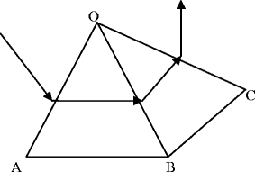
The isoline of geodesic distance tracing algorithm
-
3)
Check if the current triangle is null, then break the loop. That means that there is no iso-line on the local region.
-
4)
Trace the next triangle which has iso-points. In the step 1), the topological relationship has been preprocessed. The next triangle that is the neighbor triangle of the current triangle can be found easily with the help of the topological relationship. The next triangle is tested if there are iso-points on its edges, mark it as current.
Also in Fig. 5, the iso-line traverses the current triangle OAB from OA to OB which is labeled as out-edge. And it must traverse the neighbor triangle OBC that can be found according to their topological relationship. There is an iso-point on OC which is marked as out-edge. Add the iso-point into the iso-point array.
-
5)
If the current equals the first triangle, the tracing algorithm is terminated. A closed curve that is also the GW is obtained. And if false, turn to step 4).
Using the iso-line tracing algorithm, GWS can be extracted easily. However, with the expanding of the GW, ECC does not always describe the local region well, see Fig. 6 shows. When computing ECC, the GW is required as flat as possible. It might not be on a plane in most cases. So a flat degree is defined to restrain the expanding of GW not flat enough. The flat degree is defined as the average distance to the approximated plane of GW. How to get the approximate plane of GW? Firstly, the average of the points of GW is computed as one point on the plane. Secondly, the average normal of the triangles constructed by the average point and two neighboring point on GW is calculated as the plane normal. Finally the approximated plane is represented by the average point and the average normal. Compute the distances of points on GW to the plane and check if it is larger than a given degree, continue expanding. Else, stop GW expanding. The local region size is reduced to current geodesic distance of GW. GWS is recomputed in the reduced region correspondingly.
Fig. 6 
Two conditions that stop the GW from expanding
In addition, sometimes GW may be expanded into branches as the right picture shown in Fig. 6. If it happens, the GW expanding will stop and also the local region size is reduced to current geodesic distance of GW and GWS is recomputed in the reduced region.


3.2.3 Computation of ECC feature
After the calculation of GWS, ECC computation became easy to realize. Considering the possibility of deformation of the 3D model, a corrected source point S′ needs to be calculated before computing the ECC of every GW. According to its definition, the normal of GW and the distance between GW and the source point can be computed. GW is represented as a closed polygon. Every edge and the center of the polygon set up a triangle whose normal can be computed by cross product of any two edges of this triangle. The average of these triangles’ normal is regarded as the normal of GW. The distance of GW to the source point which is the height of the cone is computed as mentioned in the formula (3). Then a corrected source point S′ is found in the direction of GW normal with a same distance away from the GW as that of the source point. S′ and GW construct a cone and ECC is computed on this GW. After computing the ECC of every GW of the source point, ECC feature is obtained.
As mentioned before, if the source point locates at a tip position of a sharp area, the norm of ECC vector must be very large and it is nearly 0 in flat area. It is because the source point and GW are nearly coplanar. So the tip points that can be regarded as the salient points can be detected based on this characteristic. A salient point detection algorithm is proposed.
4 Salient point detection and salient feature extraction
4.1 Salient points detection
The salient points of the mesh model are the vertices with cone-curvature extremum. When people watch something the parts with curvature extremum are more impressive. The ECC feature analyzed in section 3 can depict these salient points very well. If the vertices whose ECC feature vectors has big norms, they can be regarded as the salient points.
Figure 7 gives the basic steps of the proposed salient point detection method. At first, ECC features of all the mesh vertices are extracted. The Fig. 7a shows the process of ECC feature for one vertex. The green region is the local region where GWS is extracted. GW is represented as the red closed curves. Then, a K-means cluster algorithm is employed to obtain the salient point candidates showed as the blue spheres in Fig. 7b. All the ECC features are clustered and the cluster whose cluster center has the bigger norm is selected as the candidates. As the Fig. 7b shows, all these candidates are located at the tips of the sharp area, but some of them which have the similar ECC feature concentrate in a small area. So an optimization step is needed to eliminate some neighboring candidates. All the candidates are sorted according to the norm of their ECC feature vector and saved in an array. The one with the biggest norm ranks at the top and it is marked as a salient point. Then a salient point is selected and all the candidates behind it are tested if their distances to the salient point are bigger than a given distance De, then the candidate is not a salient point and deleted from the array. The process is terminated until every salient point is tested. The left points in the array are all the salient points we detected. Figure 7c is the optimized salient points of the dog mesh model.

The process of salient point detection. First, all the ECC features are computed. Second, the features are clustered using k-means algorithm and the cluster with biggest norm of cluster center is selected as the salient point candidates. Third, an optimization step is needed to delete some candidates and obtain the salient points at last
K is an important parameter in the K-means cluster algorithm that determines the effect of salient point candidates. In our experiment, when k is set to 5, it is suitable to most of the tested models. Here the given distance is set to 0.15.
4.2 Salient region and SD descriptor
The salient region of salient point is defined as the region where GWS overlays. But not all the salient region is necessary and useful. Because of the mesh noises, some salient points with a small salient region should be eliminated. In our experiment, we obliterate by this settings: if a salient region area of a salient point is smaller than 0.3 times of the biggest salient region area, the salient point is deleted. For example, In Fig. 7c, salient point at the mouth that has very small region is deleted after the optimization step.
For building a more powerful and more precise descriptor of the 3D mesh model, besides the salient points and salient regions, the shape distribution method is also employed to extract the salient feature. Shape distribution with a lower computation, invariant to model translation, rotation and robust to noises, is very appropriate to combine with our method.
Every salient region is re-sampled by the Monte-Carlo method at first. Then shape diagram is built by counting the D2 distances of the samples. In our experiment, the sample number is 2000 and the dimension of the shape diagram is set to 64. Figure 8 shows the shape distribution plot of the salient regions. Every local salient region has two features: the ECC feature and the shape distribution feature. It can be formulated as:

The shape distribution features of the salient regions. Left is the original model with detected salient regions. And according D2 feature plot are shown in right figure. In the order of left to right: the feature curve of salient region at tail, then four curves representing four legs and two curves representing ears
5 Similarity computation
After the calculation of the salient features, every model can be indexed by a set of salient features consisting of the shape distribution and ECC. The Earth Mover’s Distance (EMD) is chosen to compute the “distance” between two sets of salient features. It tries to compute the minimum cost to transform one feature distribution to the other instead of distance, which avoids the quantification process and lowers the error. So it is often used in content-based image or 3D model retrieval as the dissimilarity function.
5.1 Earth mover’s distance
The Earth Mover’s Distance (EMD) [14] is a method to evaluate dissimilarity between two multi-dimensional distributions in some feature space where a distance measure between single features is what we called, the ground distance. The EMD “lifts” this distance from individual features to full distributions. A distribution can be represented by a set of clusters where each cluster is represented by its mean (or mode), or by the fraction of the distribution that belongs to that cluster. We call such a representation the signature of the distribution. The two signatures can have different sizes, for example, simple distributions have shorter signatures than complex ones. So EMD distance is fit for our similarity computation between the multi-dimensions salient features. Suppose two models are represented as:
Where P is the first signature with m features, p is the salient feature of the first model; Q is the second signature with n features, q is the salient feature of the second model. W is the weight of each feature.
The EMD computation is based on the solution of the transportation problem. The features in the first signature can be seemed as several suppliers, each with a given amount of goods are required to supply several consumers that is the features of the second signatures, each with a given limited capacity. For each supplier-consumer pair, the cost of transporting a single unit of goods is given. The transportation problem is then to find a least-expensive flow of goods from the suppliers to the consumers that satisfy the consumers’ demand. That is to find a flow F = [f ij ], with f ij be the flow between p i and q j that minimizes the overall cost:
\( Work\left( {P,Q,F} \right) = \sum\limits_{{i = 1}}^m {\sum\limits_{{j = 1}}^n {{f_{{ij}}}{d_{{ij}}}} } \), subject to conditions:
Once the transportation problem is solved, and we have found the optimal flow, the earth mover’s distance is defined as the work normalized by the total flow:
5.2 Similarity computation
In our experiment, the ground distance is defined as the sum of the distances of the shape distribution and ECC feature.
Where ECC is the distance between ECC features, and SD is the distance between the shape distribution. In addition, every salient feature of the model is regarded to be equal and the weight of the salient feature is defined as:
where N s is the number of the salient features.
Some models different in the global shape may have same local parts sometimes. A penalty-factor that equals max(m, n)/min(m,n) shown in formula (13) is multiplied to the EMD Distance. If the two models have similar salient features, while different numbers, their distances are enlarged.
6 Experimental results
The McGill university benchmark database (MSB) for articulated shapes[14] is chosen as the database to detect salient points and evaluate the performance of 3D model retrieval based on our proposed method. It is chosen because all the models of it are all watertight which is required to compute the ECC feature. In addition all the articulated shapes are deformable non-rigid models which are needed to demonstrate the robustness of our method to deformation. The MSB consists of 255 models in 10 categories. Models in MSB are articulated shapes, such as “human”, “octopus”, “snake”, “pliers”, and “spiders” and all of them are watertight deformable models. The categories of MSB with their number of models are shown in Table 1. Figure 9 shows some models of MSB.

The categories of the MSB database
6.1 Salient point detection
We use our salient point detection algorithm to detect salient points of the MSB models. Every vertex of the model is selected as a source point to extract its ECC feature. In this process, the size Dg of the local region where GWS is computed is set to 0.3 and the dimension of ECC feature is set to10 which means that 10 GWs is computed for every vertex on the mesh. Then all the ECC features are clustered using K-means clustering algorithm. The value of K is set to 5. All the vertices in the cluster whose cluster center has the biggest norm are selected as the salient point candidates. After the optimization step, all the salient points are obtained. Figure 10 shows some models with their detected salient points represented by a red point. Even if the model is deformed, the salient points are still detected precisely.

The salient point detection results of some MSB models. Detected salient points in the model are represented by the red spheres while GWs in yellow color surrounded them
To test the robustness of our proposed salient point detection algorithm, another experiment is done. Models of various resolutions are tested to detect the salient points. In our experiment, a mesh simplification algorithm is used to compute five various resolutions meshes with simplification rate 20%, 40%, 60%, 80% and 99.4%. The rate itself is not special and we just want to show the robustness to model resolution of our method. The vertex number and triangle number are shown in Table 2. The salient point detecting results are shown in Fig. 11.

The salient points detection experiments on various resolutions. Simplification rate labeled below models ranges from 20% to 99.4%. Even with 102 vertices at the simplification rate of 99.4% the salient points are still extracted accurately. We can infer from the results that extended cone-curvature feature is robust to model resolution
Figure 11 shows the results of salient point detection of one model in multi-resolutions. Every salient point is detected from these various resolution models, even the model with the simplification rate 99.4%. According to the definition of ECC, ECC is computed based on the cone constructed by the source point and the GW. GW is constructed by the iso-points of the geodesic distance which is robust to the resolution of the model. So our salient point detection is robust to model resolutions.
Also the salient feature is analyzed in Fig. 12. The salient feature of the left antenna for this ant mesh model is shown in plots of the shape distribution. From these curves, the salient feature stays nearly the same for the first five models. However, the last curve for the model with simplification rate 99.4% goes far away from other curves. That is partly because the model has been simplified too much and the local region shape has been changed.

The shape distribution plot of the same salient region on models in Fig. 11 are analyzed in this figure
We also tested the computation efficiency of salient point detection. Table 3 shows the time-consuming to the computation of salient point detection of various meshes. The biggest model with 14,800 vertices and 29,596 triangles costs nearly 7 min to detect the salient points. And when the model is simplified by 99.4, it only needs 0.141 s. In the total computation process, the Dijkstra algorithm to compute the geodesic distances of the local region costs the most of the computation time. When the mesh has a high resolution, the local region may have more vertices to increase the computation time of the Dijkstra algorithm. To improve the computation efficiency is what we will focus on in our future work. GPU or Cuda could also be used to improve it.
6.2 Performance of 3D model retrieval
To evaluate the effectiveness of the salient features extracted by our new method, a 3D model retrieval system is implemented to retrieve 3D models based on their similarity measured by EMD distance described in section 5.2.
The retrieval experiments are designed as following: A query model q in one category C is submitted to the system and the system will find the models in the database similar to the query model q. If the retrieved model r belongs to the category C, it is a successful retrieval. If not, it fails. The system returns a ranked list of models where the most similar models rank at the top. Figure 13 shows some retrieval results.

The retrieval results using our proposed method. It can retrieve the models that have been deformed
In our experiments all the distances between the query model and the models in database are evaluated. Each of the 255 models is used as a query and retrieved models are ranked by the distance and returned. So the ranked list is large enough to contain all the models. Here we only list the first 12 models in the ranked list. The models marked by red rectangle are the query models. And the others behind the query models are the retrieved models. According to the results, most of the retrieved models are in the same category with the query model, which means that this retrieval results are pretty well.
In addition, we can see that even if the models have been deformed, our method can still find them out exactly. For example, in Fig. 13, a hand with three fingers bended is used as a query model, and the retrieval models are all hands in different deformation. This cannot be achieved by many of the retrieval methods at present.
Another two feature descriptors are compared with our proposed method. They are D2 shape distribution methods and light filed descriptor. Shape distribution proposed by Osada [12] is computed by counting some geometry properties, such as angle, distance, area, volume. Among them, the D2 that measures the distance of any pair of model sample vertices performs well in model retrieval. D2 shape distribution is implemented by us. N vertices are sampled from the model surface at first, and the distances of (N-1)*N/2 pairs of sample vertices are counted to generate a distance diagram. N is set to 2000 and the number of diagram bins is 64.
The light field descriptor [5] is a view-based feature extraction method. 20 viewpoints located on the bounding sphere are used to generate depth images of the model. Because of symmetry, 10 images are obtained at last. Zernike moment and fourier descriptor that are used as the index of the model are extracted from these images. This descriptor uses many of the shape information and can describe the model well.
Precision- Recall plot which is well known in the literature of the content-based search and retrieval is used to evaluate the retrieval results. In the recall-precision plot, a curve closer to the upper right corner means a better retrieval performance. Ideal retrieval performance would be the precision value of 1.0 for all the recall values.
Shape distribution and Light field descriptor are two classic methods in 3D model feature extraction. They are very robust to the model noise and resolution. According to the precision-recall plot in Fig. 14, our method performs much better than the other two methods. It is reasonable to say the new descriptor proposed in this paper, the salient feature, really play a critical role than these two features popular used at present. In addition, current methods still need to be compared and we will try to continue it in our future work.

The precision-recall plot of our method and two other methods are compared with ours
7 Conclusion
This paper proposes an excellent feature descriptor, the salient feature combined with the SD descriptor, for 3D model partial retrieval. Our work can be concluded into four aspects. Firstly, cone-curvature is extended to apply on the general mesh model and the ECC (extended cone-curvature) is calculated on the general mesh. Secondly, we propose an algorithm to compute extended cone-curvature feature on the triangular mesh. Thirdly, an extended cone-curvature based algorithm is proposed to detect the salient points on the mesh model. These salient points are used to build the salient regions and salient features. Finally, an improved EMD distance is implemented to compute the similarity between models.
McGill university shape benchmark is utilized to test our proposed method. At first, salient point detection algorithm is tested on these models. The results of the salient point detection are very accurate and robust to model deformation, resolution and noise. Then, 3d model retrieval experiments are also done on the same database. Precision-recall plot is used to evaluate the retrieval results. According to the p-r plot, our proposed method is more effective and efficient than the D2 descriptor and the light field descriptor.
For further work, we would like to add the topological feature to get one more powerful feature descriptor for a much better retrieval performance. In addition, 3D partial retrieval is still a new field of research with several of unknown difficulties together with a lot of interesting points as well.. How to make use of the existing local features to do 3D partial retrieval is another future challenge work.
References
Adan A, Adan M (2004) A flexible similarity measure for 3D shapes recognition. IEEE Trans Pattern Anal Mach Intell 26, 11 (November 2004): 1507–1520. doi:10.1109/TPAMI.2004.94 http://dx.doi.org/10.1109/TPAMI.2004.94
Adán A, Adán M, Salamanca S, Merchán P. Using non local features for 3D shape grouping. SSPR/SPR 2008: 644–653
Amenta N, Bern M, Kamvysselis M (1998) A new Voronoi-based surface reconstruction algorithm. In Proceedings of the 25th annual conference on Computer graphics and interactive techniques (SIGGRAPH’98). ACM, New York, NY, USA, 415–421. doi:10.1145/280814.280947 http://doi.acm.org/10.1145/280814.280947
Ankerst M, Kastenmüller G, Kriegel H-P, Seidl T (1999) 3D shape histograms for similarity search and classification in spatial databases. In: Güting RH, Papadias D, Lochovsky FH (eds) Proceedings of the 6th International Symposium on Advances in Spatial Databases (SSD’99). Springer, London, pp 207–226
Chen D-Y, Tian X-P, Shen Y-T, Ouhyoung M. On visual similarity based 3D model retrieval, computer graphics forum (EUROGRAPHICS’03), vol. 22, no. 3, pp. 223–232, Sept. 2003
Funkhouser T, Min P, Kazhdan M, Chen J, Halderman A, Dobkin D, Jacobs D (2003) A search engine for 3D models. ACM Trans Graph 22, 1 (January 2003): 83–105. doi:10.1145/588272.588279 http://doi.acm.org/10.1145/588272.588279
Hilaga M, Shinagawa Y, Kohmura T, Kunii TL (2001) Topology matching for fully automatic similarity estimation of 3D shapes. In Proceedings of the 28th annual conference on Computer graphics and interactive techniques (SIGGRAPH’01). ACM, New York, NY, USA, 203–212. doi:10.1145/383259.383282 http://doi.acm.org/10.1145/383259.383282
Horn B (1984) Extended Gaussian image[J]. Proc IEEE 72(12):1671–1686
Kuo C-T, Cheng S-C (2007) 3D model retrieval using principal plane analysis and dynamic programming. Pattern Recogn 40, 2 (February 2007): 742–755. doi:10.1016/j.patcog.2006.06.006 http://dx.doi.org/10.1016/j.patcog.2006.06.006
Liu Y, Zha H, Qin H (2006) Shape topics: a compact representation and new algorithms for 3D partial shape retrieval. In Proceedings of the 2006 IEEE Computer Society Conference on Computer Vision and Pattern Recognition - Volume 2 (CVPR’06), Vol. 2. IEEE Computer Society, Washington, DC, USA, 2025–2032. doi:10.1109/CVPR.2006.278 http://dx.doi.org/10.1109/CVPR.2006.278
Ohbuchi R, Nakazawa M, Takei T (2003) Retrieving 3D shapes based on their appearance. In Proceedings of the 5th ACM SIGMM international workshop on Multimedia information retrieval (MIR’03). ACM, New York, NY, USA, 39–45. doi:10.1145/973264.973272 http://doi.acm.org/10.1145/973264.973272
Osada R, Funkhouser T, Chazelle B, Dobkin D (2002) Shape distributions. ACM Trans Graph 21, 4 (October 2002), 807–832. doi:10.1145/571647.571648 http://doi.acm.org/10.1145/571647.571648
Paquet E, Rioux M (1997) Nefertiti: a query by content software for three-dimensional models databases management. In Proceedings of the International Conference on Recent Advances in 3-D Digital Imaging and Modeling (NRC’97). IEEE Computer Society, Washington, DC, USA
Rubner Y, Tomasi C, Guibas LJ (1998) A metric for distributions with applications to image databases. In Proceedings of the Sixth International Conference on Computer Vision (ICCV’98). IEEE Computer Society, Washington, DC, USA
Shalom S, Shapira L, Shamir A, et al. (2008) Part analogies in sets of objects. Eurographics Workshop on 3D Object Retrieval
Shilane P, Funkhouser T (2006) Selecting distinctive 3D shape descriptors for similarity retrieval. In Proceedings of the IEEE International Conference on Shape Modeling and Applications 2006 (SMI’06). IEEE Computer Society, Washington, DC, USA, 18-. doi:10.1109/SMI.2006.34 http://dx.doi.org/10.1109/SMI.2006.34
Shilane P, Funkhouser T (2007) Distinctive regions of 3D surfaces. ACM Trans. Graph 26, 2, Article 7 (June 2007). doi:10.1145/1243980.1243981 http://doi.acm.org/10.1145/1243980.1243981
Tam GKL, Lau RWH (2007) Deformable model retrieval based on topological and geometric signatures. IEEE Trans Visual Comput Graph 13, 3 (May 2007): 470–482. doi:10.1109/TVCG.2007.1011 http://dx.doi.org/10.1109/TVCG.2007.1011
Acknowledgement
This work is partly supported by National Natural Science Foundation of China (Grant No.60873164),National High-Tech R&D Plan (Grant No. 2009AA062802), the Shandong Provincial Natural Science Foundation(Grant No.ZR2009GL014),the Scientific Research Foundation for the Excellent Middle-Aged and Youth Scientists of Shandong Province of China (Grant No.BS2010DX037), Ministry of Culture Science and Technology Innovation Project(Grant No. 46–2010),the Fundamental Research Funds for the Central Universities(Grant No. 09CX04044A, 10CX04043A,10CX04014B, 11CX04053A, 11CX06086A, 12CX06083A, 12CX06086A).
Author information
Authors and Affiliations
Corresponding author
Additional information
Research Highlights
Extends the cone-curvature and define the concept of extended cone-curvature of general mesh and gives a method to compute extended cone-curvature on triangular meshes.
An algorithm is proposed to detect the salient points based on extended cone-curvature and salient regions are extracted according to these salient points.
Extended cone-curvature feature and shape distribution feature of the salient regions are used together as the model index which performs very well in the 3D model retrieval with Earth Mover’s Distance as the similarity measure.
Rights and permissions
About this article
Cite this article
Liu, Y., Zhang, X., Li, Z. et al. Extended cone-curvature based salient points detection and 3D model retrieval. Multimed Tools Appl 64, 671–693 (2013). https://doi.org/10.1007/s11042-011-0950-7
Published:
Issue Date:
DOI: https://doi.org/10.1007/s11042-011-0950-7