Derivative-Free Local Tuning and Local Improvement Techniques Embedded in the Univariate Global Optimization

Abstract

Geometric and information frameworks for constructing global optimization algorithms are considered, and several new ideas to speed up the search are proposed. The accelerated global optimization methods automatically realize a local behavior in the promising subregions without the necessity to stop the global optimization procedure. Moreover, all the trials executed during the local phases are used also in the course of the global ones. The resulting geometric and information global optimization methods have a similar structure, and a smart mixture of new and traditional computational steps leads to 22 different global optimization algorithms. All of them are studied and numerically compared on three test sets including 120 benchmark functions and 4 applied problems.

1 Introduction

In this paper, black-box Lipschitz global optimization problems are considered in their univariate statement. Problems of this kind attract a great attention of the global optimization community. This happens because, first, there exists a huge number of real-life applications where it is necessary to solve univariate global optimization problems (see, e.g., [1–6]). This kind of problems is often encountered in scientific and engineering applications (see, e.g., [7–13]) and, in particular, in statistical applications (see, e.g., [14–19]) or in electrical engineering optimization problems (see, e.g., [20–25]). On the other hand, it is important to study one-dimensional methods because they can be successfully generalized in several ways. For instance, they can be extended to the multi-dimensional case by numerous schemes (see, for example, one-point-based, diagonal, simplicial, space-filling curves and other popular approaches in [26–31]). Another possible generalization consists in developing methods for solving problems, where the first derivative of the objective function satisfies also the Lipschitz condition with an unknown constant (see, e.g., [32–37]).

In the seventies of the twentieth century, two algorithms for solving the above-mentioned problems have been proposed in [38, 39]. The first method was introduced by Piyavskij (see also [40]) by using geometric ideas (based on the Lipschitz condition) and an a priori given overestimate of the Lipschitz constant for the objective function. The method [38] constructs a piecewise linear auxiliary function, being a minorant for the objective function, which is adaptively improved during the search. The latter algorithm [39, 41] was introduced by Strongin, who developed a statistical model that allowed him to calculate probabilities of locating global minimizers within each of the subintervals of the search interval taken into consideration. Moreover, this model provided a dynamically computed estimate of the Lipschitz constant during the process of optimization. Both the methods became sources of multiple generalizations and improvements (see, e.g., [28–30, 42, 43]) giving rise to classes of geometric and information global optimization methods.

Very often in global optimization (see, e.g., [44–46]), local techniques are used to accelerate the global search, and frequently global and local searches are realized by different methods having completely alien structures. Such a combination introduces at least two inconveniences. First, evaluations of the objective function (called hereinafter trials), executed by a local search procedure, are not used typically in the subsequent phases of the global search. Results of only some of these trials (for instance, the current best found value) can be used, and the other ones are not taken into consideration. Second, there arises the necessity to introduce both a rule that stops the global phase and starts the local one, and a rule that stops the local phase and decides whether it is necessary to restart the global search. Clearly, a premature stop of a global phase of the search can lead to the loss of the global solution, while a late stop of the global phase can slow down the search.

In this paper, both frameworks, geometric and information, are taken into consideration and a number of derivative-free techniques that were proposed to accelerate the global search are studied and compared. Several new ideas that can be used to speed up the search both in the framework of geometric and information algorithms are introduced. All the acceleration techniques have the advantage to get over both the difficulties mentioned above, namely:

• The accelerated global optimization methods automatically realize a local behavior in the promising subregions without the necessity to stop the global optimization procedure;

• All the trials executed during the local phases are used also in the course of the global ones.

It should be emphasized that the resulting geometric and information global optimization methods have a similar structure, and a smart mixture of new and traditional computational steps leads to 22 different global optimization algorithms. All of them are studied and compared on three sets of tests: the widely used set of 20 test functions taken from [47] and listed in “Appendix 1”; 100 randomly generated functions from [48]; and four functions arising in practical problems (see “Appendix 2”).

2 Acceleration Techniques

The considered global optimization problem can be formulated as follows:

$$\begin{aligned} f^*:=f(x^*)= \min f(x), \quad x \in [a,b], \end{aligned}$$

(1)

where the function f(x) satisfies the Lipschitz condition over the interval [a, b]:

$$\begin{aligned} |f(x_1)-f(x_2)| \le L|x_1 - x_2|, \quad x_1,x_2 \in [a,b], \end{aligned}$$

(2)

with the Lipschitz constant $L, 0<L<\infty$. It is supposed that the objective function f(x) can be multiextremal, non-differentiable, black-box, with an unknown Lipschitz constant L, and evaluation of f(x) even at one point is a time-consuming operation.

As mentioned in Introduction, the geometric and information frameworks are taken into consideration in this paper. The original geometric and information methods, apart from the origins of their models, have the following important difference. Piyavskij’s method requires for its correct work an overestimate of the value L that usually is hard to get in practice. In contrast, the information method of Strongin adaptively estimates L during the search. As it was shown in [49, 50] for both the methods, these two strategies for obtaining the Lipschitz information can be substituted by the so-called local tuning approach. In fact, the original methods of Piyavskij and Strongin use estimates of the global constant L during their work (the term “global” means that the same estimate is used over the whole interval [a, b]). However, the global estimate can provide a poor information about the behavior of the objective function f(x) over every small subinterval $[x_{i-1},x_i] \subset [a,b]$. In fact, when the local Lipschitz constant related to the interval $[x_{i-1}, x_i]$ is significantly smaller than the global constant L, then the methods using only this global constant or its estimate can work slowly over such an interval (see, e.g., [9, 23, 50, 51]).

In Fig. 1, an example of the auxiliary function for a Lipschitz function f(x) over [a, b] constructed by using estimations of local Lipschitz constants over subintervals of [a, b] is shown by a solid thin line; a minorant function for f(x) over [a, b] constructed by using an overestimate of the global Lipschitz constant is represented by a dashed line. Note that the former piecewise function estimates the behavior of f(x) over [a, b] more accurately than the latter one, especially over subintervals where the corresponding local Lipschitz constants are smaller than the global one.

Fig. 1

An auxiliary function (solid thin line) and a minorant function (dashed line) for a Lipschitz function f(x) over [a, b], constructed by using estimates of local Lipschitz constants and by using the global Lipschitz constant, respectively (trial values are circled)

The local tuning technique proposed in [49, 50] adaptively estimates local Lipschitz constants at different subintervals of the search region during the course of the optimization process. Estimates $l_i$ of local Lipschitz constants $L_i$ are computed for each interval $[x_{i-1}, x_i], i=2,\ldots ,k,$ as follows:

$$\begin{aligned} l_i = r \cdot \max \{\lambda _i, \gamma _i, \xi \}, \end{aligned}$$

(3)

where

$$\begin{aligned} \lambda _i= & {} \max \{H_{i-1}, H_i, H_{i+1}\}, \quad \ i=2,\ldots ,k, \end{aligned}$$

(4)

$$\begin{aligned} H_i= & {} \frac{|z_i - z_{i-1}|}{x_i - x_{i-1}},\quad i=2,\ldots ,k,\end{aligned}$$

(5)

$$\begin{aligned} H^k= & {} \max \{H_i: i=2,\ldots ,k\}. \end{aligned}$$

(6)

Here, $z_i = f(x_i), i=1,\ldots ,k,$ i.e., values of the objective function calculated at the previous iterations at the trial points $x_i, i=1,\ldots ,k,$ (when $i=2$ and $i=k$ only $H_2,$ $H_3$ and $H_{k-1}, H_k$, should be considered, respectively). The value $\gamma _i$ is calculated as follows:

$$\begin{aligned} \gamma _i = H^k \frac{(x_i-x_{i-1})}{ X^{\max }}, \end{aligned}$$

(7)

with $H^k$ from (6) and

$$\begin{aligned} X^\mathrm{max} = \max \{x_i-x_{i-1}: \ i=2,\ldots ,k \}. \end{aligned}$$

(8)

Let us give an explanation of these formulae. The parameter $\xi >0$ from (3) is a small number, that is required for a correct work of the local tuning at initial steps of optimization, where it can happen that $\max \{\lambda _i, \gamma _i \}=0$; $r>1$ is the reliability parameter. The two components, $\lambda _i$ and $\gamma _i$, are the main players in (3). They take into account, respectively, the local and the global information obtained during the previous iterations. When the interval $[x_{i-1}, x_i]$ is large, the local information represented by $\lambda _i$ can be not reliable and the global part $\gamma _i$ has a decisive influence on $l_i$ thanks to (3) and (7). In this case $\gamma _i \rightarrow H^k$; namely, it tends to the estimate of the global Lipschitz constant L. In contrast, when $[x_{i-1}, x_i]$ is small, then the local information becomes relevant, the estimate $\gamma _i$ is small for small intervals (see 7), and the local component $\lambda _i$ assumes the key role. Thus, the local tuning technique automatically balances the global and the local information available at the current iteration. It has been proved for a number of global optimization algorithms that the usage of the local tuning can accelerate the search significantly (see [9, 10, 23, 33, 50, 52–54]). This local tuning strategy will be called “Maximum” Local Tuning hereinafter.

Recently, a new local tuning strategy called hereinafter “Additive” Local Tuning has been proposed in [11, 55, 56] for certain information algorithms. It proposes to use the following additive convolution instead of (3):

$$\begin{aligned} l_i = r \cdot \max \left\{ \frac{1}{2}(\lambda _i + \gamma _i), \xi \right\} , \end{aligned}$$

(9)

where $r, \xi , \lambda _i$ and $\gamma _i$ have the same meaning as in (3). The first numerical examples executed in [11, 55] have shown a very promising performance of the “Additive” Local Tuning. These results induced us to execute in the present paper a broad experimental testing and a theoretical analysis of the “Additive” Local Tuning. In particular, geometric methods using this technique are proposed here (remind that the authors of [11, 55] have introduced it in the framework of information methods only). During our study, some features suggesting a careful usage of this technique have been discovered, especially in cases where it is applied to geometric global optimization methods.

In order to start our analysis of the “Additive” Local Tuning, let us remind (see, e.g., [8, 9, 23, 30, 38, 39]) that in both the geometric and the information univariate algorithms, an interval $[x_{t-1},x_t]$ is chosen in a certain way at the $(k+1)$th iteration of the optimization process and a new trial point, $x^{k+1}$, where the $(k+1)$th evaluation of f(x) is executed, is computed as follows:

$$\begin{aligned} x^{k+1} = \frac{x_t + x_{t-1}}{2} - \frac{z_t - z_{t-1}}{2l_t}. \end{aligned}$$

(10)

For a correct work of this kind of algorithms, it is necessary that $x^{k+1}$ is such that $x^{k+1} \in ]x_{t-1},x_t[$. It is easy to see that the necessary condition for this inclusion is $l_t> H_t$, where $H_t$ is calculated following (5). Notice that $l_t$ is obtained by using (9), where the sum of two addends plays the leading role. Since the estimate $\gamma _i$ is calculated as shown in (7), it can be very small for small intervals, creating so the possibility of occurrence of the situation $l_t \le H_t$ and, consequently, $x^{k+1} \notin ]x_{t-1},x_t[$. Obviously, by increasing the value of the parameter r, this situation can be easily avoided and the method should be restarted. In fact, in information algorithms where $r \ge 2$ is usually used, this risk is less pronounced, while in geometric methods where $r >1$ is applied it becomes more probable. On the other hand, it is well known in Lipschitz global optimization (see, e.g., [8, 9, 23, 30]) that increasing the parameter r can slow down the search. In order to understand better the functioning of the “Additive” Local Tuning, it is broadly tested in Sect. 4 together with other competitors.

The analysis provided above shows that the usage of the “Additive” Local Tuning can become tricky in some cases. In order to avoid the necessity to check the satisfaction of the condition $x^{k+1} \in ]x_{t-1},x_t[$ at each iteration, we propose a new strategy called the “Maximum-Additive” Local Tuning where, on the one hand, this condition is satisfied automatically and, on the other hand, advantages of both the local tuning techniques described above are incorporated in the unique strategy. This local tuning strategy calculates the estimate $l_i$ of the local Lipschitz constants as follows:

$$\begin{aligned} l_i = r \cdot \max \left\{ H_i, \frac{1}{2}(\lambda _i + \gamma _i), \xi \right\} , \end{aligned}$$

(11)

where $r, \xi , H_i, \lambda _i$ and $\gamma _i$ have the usual meaning. It can be seen from (11) that this strategy both maintains the additive character of the convolution and satisfies condition $l_i> H_i$. The latter condition provides that in case the interval $[x_{i-1}, x_i]$ is chosen for subdivision (i.e., $t:=i$ is assigned), the new trial point $x^{k+1}$ will belong to $]x_{t-1},x_t[$. Notice that in (11) the equal usage of the local and global estimate is applied. Obviously, a more general scheme similar to (9) and (11) can be used, where $\frac{1}{2}$ is substituted by different weights for the estimates $\lambda _i$ and $\gamma _i$, for example, as follows:

$$\begin{aligned} l_i = r \cdot \max \left\{ H_i, \frac{\lambda _i}{r} + \frac{r-1}{r}\gamma _i, \xi \right\} \end{aligned}$$

[$r,~H_i,~\lambda _i,~\gamma _i$ and $\xi$ are as in (11)].

Let us now present another acceleration idea that will be introduced formally in next Section. It consists in the following observation, related to global optimization problems with a fixed budget of possible evaluations of the objective function f(x), i.e., when only, for instance, 100 or 1,000,000 evaluations of f(x) are allowed. In these problems, it is necessary to obtain the best possible value of f(x) as soon as possible. Suppose that $f^*_k$ is the best value (the record value) obtained after k iterations. If a new value $f(x^{k+1})<f^*_k$ has been obtained, then it can make sense to try to improve this value locally, instead of continuing the usual global search phase. As was already mentioned, traditional methods stop the global procedure and start a local descent: Trials executed during this local phase are not then used by the global search since the local method has usually a completely different nature.

Here, we propose two local improvement techniques, the “optimistic” and the “pessimistic” one that perform the local improvement within the global optimization scheme. The optimistic method alternates the local steps with the global ones, and if during the local descent a new promising local minimizer is not found, then the global method stops when a local stopping rule is satisfied. The pessimistic strategy does the same until the satisfaction of the required accuracy on the local phase and then switches to the global phase where the trials performed during the local phase are also taken into consideration.

3 Numerical Methods and Their Convergence Study

All the methods described in this Section have a similar structure and belong to the class of “Divide the Best” global optimization algorithms introduced in [57] (see also [9]; for methods using the “Additive” Local Tuning this holds if the parameter r is such that $l_{i(k)} > rH_{i(k)}$ for all i and k). The algorithms differ in the following:

• Methods are either geometric or information;

• Methods differ in the way the Lipschitz information is used: an a priori estimate, a global estimate and a local tuning;

• In cases where a local tuning is applied, methods use 3 different strategies: Maximum, Additive and Maximum-Additive;

• In cases where a local improvement is applied, methods use either the optimistic or the pessimistic strategy.

Let us describe the general scheme (GS) of the methods used in this work. A concrete algorithm will be obtained by specifying one of the possible implementations of Steps 2–4 in this GS.

• Step 0 Initialization. Execute first two trials at the points a and b, i.e., $x^1 := a, z^1:=f(a)$ and $x^2 := b, z^2:=f(b)$. Set the iteration counter $k := 2$.

  Let flag be the local improvement switch to alternate global search and local improvement procedures; set its initial value $flag:=0$. Let $i_{\min }$ be an index (being constantly updated during the search) of the current record point, i.e., $z_{i_{\min }} = f(x_{i_{\min }}) \le f(x_i), i = 1,\ldots ,k$ (if the current minimal value is attained at several trial points, then the smallest index is accepted as $i_{\min }$).

  Suppose that $k \ge 2$ iterations of the algorithm have already been executed. The iteration $k + 1$ consists of the following steps.

• Step 1 Reordering. Reorder the points $x^1,\ldots ,x^k$ (and the corresponding function values $z^1,\ldots ,z^k$) of previous trials by subscripts so that

  $$\begin{aligned} a = x_1< \cdots < x_k = b, \qquad z_i=f(x_i), \, i=1,\ldots ,k. \end{aligned}$$

• Step 2 Estimates of the Lipschitz constant. Calculate the current estimates $l_i$ of the Lipschitz constant for each subinterval $[x_{i-1},x_{i}], i=2,\ldots ,k$, in one of the following ways.

  • Step 2.1 A priori given estimate. Take an a priori given estimate $\hat{L}$ of the Lipschitz constant for the whole interval [a, b], i.e., set $l_i := \hat{L}$.

  • Step 2.2 Global estimate. Set $l_i := r \cdot \max \{ H^k, \xi \},$ where r and $\xi$ are two parameters with $r>1$ and $\xi$ sufficiently small, $H^k$ is from (6).

  • Step 2.3 “Maximum” Local Tuning. Set $l_i$ following (3).

  • Step 2.4 “Additive” Local Tuning. Set $l_i$ following (9).

  • Step 2.5 “Maximum-Additive” Local Tuning. Set $l_i$ following (11).

• Step 3 Calculation of characteristics. Compute for each subinterval $[x_{i-1},x_i], i=2,\ldots ,k$, its characteristic $R_i$ (see, e.g., [5, 11]) by using one of the following rules.

  • Step 3.1 Geometric methods.

    $$\begin{aligned} R_i = \frac{z_i + z_{i-1}}{2} - l_i \frac{x_i - x_{i-1}}{2}. \end{aligned}$$

  • Step 3.2 Information methods.

    $$\begin{aligned} R_i = 2(z_i + z_{i-1}) - l_i(x_i - x_{i-1}) - \frac{(z_i - z_{i-1})^2}{l_i (x_i - x_{i-1})}. \end{aligned}$$

• Step 4 Subinterval selection. Determine subinterval $[x_{t-1},x_t], t=t(k)$, for performing next trial by using one of the following rules.

  • Step 4.1 Global phase. Select the subinterval $[x_{t-1},x_t]$ corresponding to the minimal characteristic, i.e., such that $t = \arg \min _{i=2,\ldots ,k} R_i$.

  • Steps 4.2–4.3 Local improvement.

    

    The subsequent part of this Step differs for two local improvement techniques.

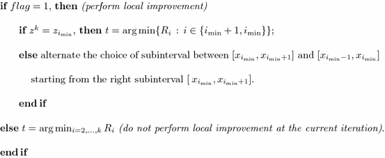
    • Step 4.2 Pessimistic local improvement.

      

    • Step 4.3 Optimistic local improvement.

      $$\begin{aligned}&\hbox {Set } \hbox {flag}:= \hbox {NOT(flag) }(\hbox {switch the local/global flag: the accuracy of local}\\&\hbox {search is not separately checked in this strategy}). \end{aligned}$$

• Step 5 Global stopping criterion. If

  $$\begin{aligned} x_t - x_{t-1} \le \varepsilon , \end{aligned}$$

  (13)

  where $\varepsilon >0$ is a given accuracy of the global search, then Stop and take as an estimate of the global minimum $f^*$ the value $f_k^* = \min _{i=1,\ldots ,k} \{z_i\}$ obtained at a point $x_k^* = \arg \min _{i=1,\ldots ,k} \{z_i\}$.

• Otherwise, go to Step 6.

• Step 6 New trial. Execute next trial at the point $x^{k+1}$ from (10): $z^{k+1}:=f(x^{k+1})$. Increase the iteration counter $k:=k+1$, and go to Step 1.

Table 1 Description of the methods considered in the paper, the signs “+” show a combination of implementations of Steps 2–4 in the GS for each method

All the Lipschitz global optimization methods considered in the paper are summarized in Table 1, from which concrete implementations of Steps 2–4 in the GS can be individuated. As shown experimentally in Sect. 4, the methods using an a priori given estimate of the Lipschitz constant or its global estimate lose, as a rule, in comparison with methods using local tuning techniques, in terms of the trials performed to approximate the global solutions to problems. Therefore, local improvement accelerations (Steps 4.2–4.3 of the GS) were implemented for methods using local tuning strategies only. In what follows, the methods from Table 1 are furthermore specified (for the methods known in the literature, the respective references are provided).

• 1. Geom-AL Piyavskij’s method with the a priori given Lipschitz constant (see [38, 40] and [9, 51] for generalizations and discussions): GS with Step 2.1, Step 3.1 and Step 4.1.

• 2. Geom-GL Geometric method with the global estimate of the Lipschitz constant (see [9]): GS with Step 2.2, Step 3.1 and Step 4.1.

• 3. Geom-LTM Geometric method with the “Maximum” Local Tuning (see [9, 23, 50]): GS with Step 2.3, Step 3.1 and Step 4.1.

• 4. Geom-LTA Geometric method with the “Additive” Local Tuning: GS with Step 2.4, Step 3.1 and Step 4.1.

• 5. Geom-LTMA Geometric method with the “Maximum-Additive” Local Tuning: GS with Step 2.5, Step 3.1 and Step 4.1.

• 6. Geom-LTIMP Geometric method with the “Maximum” Local Tuning and the pessimistic strategy of the local improvement (see [9, 37]): GS with Step 2.3, Step 3.1 and Step 4.2.

• 7. Geom-LTIAP Geometric method with the “Additive” Local Tuning and the pessimistic strategy of the local improvement: GS with Step 2.4, Step 3.1 and Step 4.2.

• 8. Geom-LTIMAP Geometric method with the “Maximum-Additive” Local Tuning and the pessimistic strategy of the local improvement: GS with Step 2.5, Step 3.1 and Step 4.2.

• 9. Geom-LTIMO Geometric method with the “Maximum” Local Tuning and the optimistic strategy of the local improvement: GS with Step 2.3, Step 3.1 and Step 4.3.

• 10. Geom-LTIAO Geometric method with the “Additive” Local Tuning and the optimistic strategy of the local improvement: GS with Step 2.4, Step 3.1 and Step 4.3.

• 11. Geom-LTIMAO Geometric method with the “Maximum-Additive” Local Tuning and the optimistic strategy of the local improvement: GS with Step 2.5, Step 3.1 and Step 4.3.

• 12. Inf-AL Information method with the a priori given Lipschitz constant (see [9]): GS with Step 2.1, Step 3.2 and Step 4.1.

• 13. Inf-GL Strongin’s information-statistical method with the global estimate of the Lipschitz constant (see [23, 39, 41]): GS with Step 2.2, Step 3.2 and Step 4.1.

• 14. Inf-LTM Information method with the “Maximum” Local Tuning (see [23, 30, 49]): GS with Step 2.3, Step 3.2 and Step 4.1.

• 15. Inf-LTA Information method with the “Additive” Local Tuning (see [11, 55]): GS with Step 2.4, Step 3.2 and Step 4.1.

• 16. Inf-LTMA Information method with the “Maximum-Additive” Local Tuning: GS with Step 2.5, Step 3.2 and Step 4.1.

• 17. Inf-LTIMP Information method with the “Maximum” Local Tuning and the pessimistic strategy of the local improvement [30, 58]: GS with Step 2.3, Step 3.2 and Step 4.2.

• 18. Inf-LTIAP Information method with the “Additive” Local Tuning and the pessimistic strategy of the local improvement: GS with Step 2.4, Step 3.2 and Step 4.2.

• 19. Inf-LTIMAP Information method with the “Maximum-Additive” Local Tuning and the pessimistic strategy of the local improvement: GS with Step 2.5, Step 3.2 and Step 4.2.

• 20. Inf-LTIMO Information method with the “Maximum” Local Tuning and the optimistic strategy of the local improvement: GS with Step 2.3, Step 3.2 and Step 4.3.

• 21. Inf-LTIAO Information method with the “Additive” Local Tuning and the optimistic strategy of the local improvement: GS with Step 2.4, Step 3.2 and Step 4.3.

• 22. Inf-LTIMAO Information method with the “Maximum-Additive” Local Tuning and the optimistic strategy of the local improvement: GS with Step 2.5, Step 3.2 and Step 4.3.

Let us spend a few words regarding convergence of the methods belonging to the GS. To do this, we study an infinite trial sequence $\{x^k\}$ generated by an algorithm belonging to the general scheme GS for solving the problem (1), (2) with $\delta =0$ from (12) and $\varepsilon =0$ from (13).

Theorem 3.1

Assume that the objective function f(x) satisfies the Lipschitz condition (2) with a finite constant $L>0$, and let $x'$ be any limit point of $\{x^k\}$ generated by an algorithm belonging to the GS that does not use the “Additive” Local Tuning and works with one of the estimates (3), (6), (11). Then, the following assertions hold:

• 1. If $x' \in ]a,b[$, then convergence to $x'$ is bilateral, i.e., there exist two infinite subsequences of $\{x^k\}$ converging to $x'$: one from the left, the other from the right;

• 2. $f(x^k) \ge f(x')$, for all trial points $x^k, k\ge 1$;

• 3. If there exists another limit point $x''\ne x'$, then $f(x'')=f(x')$;

• 4. If the function f(x) has a finite number of local minima in [a, b], then the point $x'$ is locally optimal;

• 5. (Sufficient conditions for convergence to a global minimizer). Let $x^*$ be a global minimizer of f(x). If there exists an iteration number $k^*$ such that for all $k>k^*$, then the inequality

  $$\begin{aligned} l_{j(k)} > L_{j(k)} \end{aligned}$$

  (14)

  holds, where $L_{j(k)}$ is the Lipschitz constant for the interval $[x_{j(k)-1}, x_{j(k)}]$ containing $x^*$, and $l_{j(k)}$ is its estimate. Then, the set of limit points of the sequence $\{x^k\}$ coincides with the set of global minimizers of the function f(x).

Proof

Since all the methods mentioned in the Theorem belong to the “Divide the Best” class of global optimization algorithms introduced in [57], the proofs of assertions 1–5 can be easily obtained as particular cases of the respective proofs in [9, 57]. $\square$

Corollary 3.1

Assertions 1–5 hold for methods belonging to the GS and using the “Additive” Local Tuning if the condition $l_{i(k)} > rH_{i(k)}$ is fulfilled for all i and k.

Proof

Fulfillment of the condition $l_{i(k)} > rH_{i(k)}$ ensures that: (i) Each new trial point $x^{k+1}$ belongs to the interval $(x_{t-1},x_t)$ chosen for partitioning; (ii) the distances $x^{k+1}-x_{t-1}$ and $x_t-x^{k+1}$ are finite. The fulfillment of these two conditions implies that the methods belong to the class of “Divide the Best” global optimization algorithms, and therefore, proofs of assertions 1–5 can be easily obtained as particular cases of the respective proofs in [9, 57]. $\square$

Note that in practice, since both $\varepsilon$ and $\delta$ assume finite positive values, methods using the optimistic local improvement can miss the global optimum and stop in the $\delta$-neighborhood of a local minimizer (see Step 4 of the GS).

Next Theorem ensures existence of the values of the reliability parameter r satisfying condition (14), providing so the fact that all global minimizers of f(x) will be determined by the proposed methods without using the a priori known Lipschitz constant.

Theorem 3.2

For any function f(x) satisfying the Lipschitz condition (2) with $L < \infty$ and for methods belonging to the GS and using one of the estimates (3), (6), (9), (11) there exists a value $r^*$ such that, for all $r>r^*$, condition (14) holds.

Proof

It follows from, (3), (6), (9), (11), and the finiteness of $\xi > 0$ that approximations of the Lipschitz constant $l_i$ in the methods belonging to the GS are always positive. Since L in (2) is finite and any positive value of the parameter r can be chosen in (3), (6), (9), (11), it follows that there exists an $r^*$ such that condition (14) will be satisfied for all global minimizers for $r>r^*$. $\square$

4 Numerical Experiments

Seven series of numerical experiments were executed on the following three sets of test functions to compare 22 global optimization methods described in Sect. 3:

• 1. The widely used set of 20 test functions from [47] reported in “Appendix 1”;

• 2. 100 randomly generated Pintér’s functions from [48];

• 3. Four functions originated from practical problems (see “Appendix 2”): First two problems are from [9, p. 113] and the other two functions from [17] (see also [18]).

Geometric and information methods with and without the local improvement techniques (optimistic and pessimistic) were tested in these experimental series. In all the experiments, the accuracy of the global search was chosen as $\varepsilon =10^{-5}(b-a)$, where [a, b] is the search interval. The accuracy of the local search was set as $\delta =\varepsilon$ in the algorithms with the local improvement. Results of numerical experiments are reported in Tables 2, 3, 4, 5, 6, 7, 8 and 9, where the number of function trials executed until the satisfaction of the stopping rule is presented for each considered method (the best results for the methods within the same class are shown in bold).

Table 2 Number of trials performed by the considered geometric methods without the local improvement on 20 tests from “Appendix 1”

The first series of numerical experiments was carried out with geometric and information algorithms without the local improvement on 20 test functions given in “Appendix 1.” Parameters of the geometric methods Geom-AL, Geom-GL, Geom-LTM, Geom-LTA and Geom-LTMA were chosen as follows. For the method Geom-AL, the estimates of the Lipschitz constants were computed as the maximum between the values calculated as relative differences on $10^{-7}$-grid and the values given in [47]. For the methods Geom-GL, Geom-LTM and Geom-LTMA, the reliability parameter $r = 1.1$ was used as recommended in [9]. The technical parameter $\xi = 10^{-8}$ was used for all the methods with the local tuning (Geom-LTM, Geom-LTA and Geom-LTMA). For the method Geom-LTA, the parameter r was increased with the step equal to 0.1, starting from $r=1.1$ until all 20 test problems were solved (i.e., for all the problems the algorithm stopped in the $\varepsilon$-neighborhood of a global minimizer). This situation happened for $r=1.8$: The corresponding results are shown in the column Geom-LTA of Table 2.

Table 3 Number of trials performed by the considered information methods without the local improvement on 20 tests from “Appendix 1”

As can be seen from Table 2, the performance of the method Geom-LTMA was better with respect to the other geometric algorithms tested. The experiments also showed that the additive convolution (Geom-LTA) did not guarantee the proximity of the found solution to the global minimum with the common value $r = 1.1$. With an increased value of the reliability parameter r, the average number of trials performed by this method on 20 tests was also slightly worse than that of the method with the maximum convolution (Geom-LTM), but better than the averages of the methods using global estimates of the Lipschitz constants (Geom-AL and Geom-GL).

Results of numerical experiments with information methods without the local improvement techniques (methods Inf-AL, Inf-GL, Inf-LTM, Inf-LTA and Inf-LTMA) on the same 20 tests from “Appendix 1” are shown in Table 3. Parameters of the information methods were chosen as follows. The estimates of the Lipschitz constants for the method Inf-AL were the same as for the method Geom-AL. The reliability parameter $r = 2$ was used in the methods Inf-GL, Inf-LTM and Inf-LTMA, as recommended in [9, 23, 39]. For all the information methods with the local tuning techniques (Inf-LTM, Inf-LTA and Inf-LTMA), the value $\xi = 10^{-8}$ was used. For the method Inf-LTA, the parameter r was increased (starting from $r=2$) up to the value $r=2.3$ when all 20 test problems were solved.

As can be seen from Table 3, the performance of the method Inf-LTMA was better (as also verified for its geometric counterpart) with respect to the other information algorithms tested. The experiments also showed that the average number of trials performed by the Inf-LTA method with $r=2.3$ on 20 tests was better than that of the method with the maximum convolution (Inf-LTM).

Table 4 Results of numerical experiments with the considered geometric and information methods without the local improvement on 100 Pintér’s test functions from [48]

The second series of experiments (see Table 4) was executed on the class of 100 Pintér’s test functions from [48] with all geometric and information algorithms without the local improvement (i.e., all the methods used in the first series of experiments). Parameters of the methods Geom-AL, Geom-GL, Geom-LTM, Geom-LTMA, and Inf-AL, Inf-GL, Inf-LTM and Inf-LTMA were the same as in the first experimental series ($r = 1.1$ for all the geometric methods and $r = 2$ for the information methods). The reliability parameter for the method Geom-LTA was increased from $r=1.1$ to $r = 1.8$ (when all 100 problems were solved). All the information methods were able to solve all 100 test problems with $r=2$ (see Table 4). The average performance of the Geom-LTMA and the Inf-LTA methods was the best among the other considered geometric and information algorithms, respectively.

Table 5 Number of trials performed by the considered geometric and information methods without the local improvement on four test functions from “Appendix 2”

The third series of the experiments (see Table 5) was carried out on four applied test problems from [9] and [17] (see “Appendix 2”). All the methods without the local improvement used in the previous two series of experiments (Geom-AL, Geom-GL, Geom-LTM, Geom-LTA, Geom-LTMA and Inf-AL, Inf-GL, Inf-LTM, Inf-LTA, Inf-LTMA) were tested, and all the parameters for these methods were the same as above, except the reliability parameters of the methods Geom-LTA and Inf-LTA. Particularly, the applied problem 4 was not solved by the Geom-LTA method with $r=1.1$. With the increased value $r=1.8$, the obtained results (reported in Table 5) of this geometric method were worse than the results of the other geometric methods with the local tuning (Geom-LTM and Geom-LTMA). The method Inf-LTA solved all the four applied problems also with a higher value $r = 2.3$ and was outrun by the Inf-LTMA method (the latter one produced the best average result among all the competitors; see Table 5).

Table 6 Number of trials performed by the considered geometric and information methods with the optimistic local improvement on 20 tests from “Appendix 1”

Table 7 Number of trials performed by the considered geometric and information methods with the pessimistic local improvement on 20 tests from “Appendix 1”

In the following several series of experiments, the local improvement techniques were compared on the same three sets of test functions. In the fourth series (see Table 6), six methods (geometric and information) with the optimistic local improvement (methods Geom-LTIMO, Geom-LTIAO, Geom-LTIMAO and Inf-LTIMO, Inf-LTIAO and Inf-LTIMAO) were compared on the class of 20 test functions from [47] (see “Appendix 1”). The reliability parameter $r = 1.1$ was used for the methods Geom-LTIMO and Geom-LTIMAO, and $r=2$ was used for the method Inf-LTIMO. For the method Geom-LTIAO, r was increased to 1.6, and for the methods Inf-LTIMAO and Inf-LTIAO, r was increased to 2.3. As can be seen from Table 6, the best average result among all the algorithms was shown by the method Geom-LTIMAO (while the Inf-LTIMAO was the best in average among the considered information methods).

In the fifth series of experiments, six methods (geometric and information) using the pessimistic local improvement were compared on the same 20 test functions. The obtained results are presented in Table 7. The usual values $r=1.1$ and $r=2$ were used for the geometric (Geom-LTIMP and Geom-LTIMAP) and the information (Inf-LTIMP and Inf-LTIMAP) methods, respectively. The values of the reliability parameter ensuring the solution to all the test problems in the case of methods Geom-LTIAP and Inf-LTIAP were set as $r = 1.8$ and $r = 2.3$, respectively. As can be seen from Table 7, the “Maximum” and the “Maximum-Additive” local tuning techniques were more stable and generally allowed us to find the global solution for all test problems without increasing r. Moreover, the methods Geom-LTIMAP and Inf-LTIMAP showed the best performance with respect to the other techniques in the same geometric and information classes, respectively.

Table 8 Results of numerical experiments with the considered geometric and information methods with the local improvement techniques on 100 Pintér’s test functions from [48]

Table 9 Number of trials performed by the considered geometric and information methods with the local improvement techniques on four test functions from “Appendix 2”

In the sixth series of experiments, the local improvement techniques were compared on the class of 100 Pintér’s functions. The obtained results are presented in Table 8. The values of the reliability parameter r for all the methods were increased, starting from $r=1.1$ for the geometric methods and $r=2$ for the information methods, until all 100 problems from the class were solved. It can be seen from Table 8 that the best average number of trials for both the optimistic and pessimistic strategies was almost the same (36.90 and 37.21 in the case of information methods and 45.76 and 48.24 in the case of geometric methods, for the optimistic and for the pessimistic strategies, respectively). However, the pessimistic strategy seemed to be more stable since its reliability parameter (needed to solve all the problems) generally remained smaller than that of the optimistic strategy. In average, the Geom-LTMA and the Inf-LTA methods were the best among the other considered geometric and information algorithms, respectively.

Finally, the last, seventh, series of the experiments (see Table 9) was executed on the class of four applied test problems from “Appendix 2,” where in the third column the values of the reliability parameter used to solve all the problems are also indicated. Again, as in the previous experiments, the pessimistic local improvement strategy seemed to be more stable in the case of this test set, since the optimistic strategy required a significant increase of the parameter r to determine global minimizers of these applied problems (although the best average value obtained by the optimistic Geom-LTIAO method was smaller that that of the best pessimistic Geom-LTIMAP method, see the last column in Table 9).

5 Conclusions

Univariate derivative-free global optimization has been considered in the paper, and several numerical methods belonging to the geometric and information classes of algorithms have been proposed and analyzed. New acceleration techniques to speed up the global search have been introduced. They can be used in both the geometric and information frameworks. All of the considered methods automatically switch from the global optimization to the local one and back, avoiding so the necessity to stop the global phase manually. An original mixture of new and traditional computational steps has allowed the authors to construct 22 different global optimization algorithms having, however, a similar structure. As shown, 9 instances of this mixture can lead to known global optimization methods, and the remaining 13 methods described in the paper are new. All of them have been studied theoretically and numerically compared on 124 theoretical and applied benchmark tests. It has been shown that the introduced acceleration techniques allowed the global optimization methods to significantly speed up the search with respect to some known algorithms.

Appendices

Appendix 1

See Table 10.

Table 10 Twenty test functions from [47] used in numerical experiments

Appendix 2

See Table 11.

Table 11 Four one-dimensional test functions taken from practical applications

References

Kvasov, D.E., Sergeyev, Y.D.: Lipschitz global optimization methods in control problems. Autom. Remote Control 74(9), 1435–1448 (2013)
Hamacher, K.: On stochastic global optimization of one-dimensional functions. Phys. A Stat. Mech. Appl. 354, 547–557 (2005)
Johnson, D.E.: Introduction to Filter Theory. Prentice Hall Inc., New Jersey (1976)
Žilinskas, A.: Optimization of one-dimensional multimodal functions: algorithm AS 133. Appl. Stat. 23, 367–375 (1978)
Sergeyev, Y.D., Grishagin, V.A.: A parallel algorithm for finding the global minimum of univariate functions. J. Optim. Theory Appl. 80(3), 513–536 (1994)
Kvasov, D.E., Menniti, D., Pinnarelli, A., Sergeyev, Y.D., Sorrentino, N.: Tuning fuzzy power-system stabilizers in multi-machine systems by global optimization algorithms based on efficient domain partitions. Electr. Power Syst. Res. 78(7), 1217–1229 (2008)
Kvasov, D.E., Sergeyev, Y.D.: Deterministic approaches for solving practical black-box global optimization problems. Adv. Eng. Softw. 80, 58–66 (2015)
Pintér, J.D.: Global Optimization in Action (Continuous and Lipschitz Optimization: Algorithms, Implementations and Applications). Kluwer Academic Publishers, Dordrecht (1996)
Sergeyev, Y.D., Kvasov, D.E.: Diagonal Global Optimization Methods. Fizmatlit, Moscow (2008). (in Russian)
Sergeyev, Y.D., Kvasov, D.E., Khalaf, F.M.H.: A one-dimensional local tuning algorithm for solving GO problems with partially defined constraints. Optim. Lett. 1(1), 85–99 (2007)
Strongin, R.G., Gergel, V.P., Grishagin, V.A., Barkalov, K.A.: Parallel Computing for Global Optimization Problems. Moscow University Press, Moscow (2013). (in Russian)
Liuzzi, G., Lucidi, S., Piccialli, V., Sotgiu, A.: A magnetic resonance device designed via global optimization techniques. Math. Program. 101(2), 339–364 (2004)
Daponte, P., Grimaldi, D., Molinaro, A., Sergeyev, Y.D.: An algorithm for finding the zero-crossing of time signals with Lipschitzean derivatives. Measurement 16(1), 37–49 (1995)
Calvin, J.M., Žilinskas, A.: One-dimensional global optimization for observations with noise. Comput. Math. Appl. 50(1–2), 157–169 (2005)
Calvin, J.M., Chen, Y., Žilinskas, A.: An adaptive univariate global optimization algorithm and its convergence rate for twice continuously differentiable functions. J. Optim. Theory Appl. 155(2), 628–636 (2012)
Gergel, V.P.: A global search algorithm using derivatives. In: Neymark, Y.I. (ed.) Systems Dynamics and Optimization, pp. 161–178. N. Novgorod University Press, Novgorod (1992). (in Russian)
Gillard, J.W., Zhigljavsky, A.A.: Optimization challenges in the structured low rank approximation problem. J. Glob. Optim. 57(3), 733–751 (2013)
Gillard, J.W., Kvasov, D.E.: Lipschitz optimization methods for fitting a sum of damped sinusoids to a series of observations. Stat. Interface (2016, in press)
Žilinskas, A.: A one-step worst-case optimal algorithm for bi-objective univariate optimization. Optim. Lett. 8(7), 1945–1960 (2014)
Daponte, P., Grimaldi, D., Molinaro, A., Sergeyev, Y.D.: Fast detection of the first zero-crossing in a measurement signal set. Measurement 19(1), 29–39 (1996)
Molinaro, A., Sergeyev, Y.D.: Finding the minimal root of an equation with the multiextremal and nondifferentiable left-hand part. Numer. Algorithms 28(1–4), 255–272 (2001)
Sergeyev, Y.D., Daponte, P., Grimaldi, D., Molinaro, A.: Two methods for solving optimization problems arising in electronic measurements and electrical engineering. SIAM J. Optim. 10(1), 1–21 (1999)
Strongin, R.G., Sergeyev, Y.D.: Global Optimization with Non-Convex Constraints: Sequential and Parallel Algorithms. Kluwer Academic Publishers, Dordrecht (2000). (2nd ed., 2012; 3rd ed., 2014, Springer, New York)
Casado, L.G., García, I., Sergeyev, Y.D.: Interval algorithms for finding the minimal root in a set of multiextremal non-differentiable one-dimensional functions. SIAM J. Sci. Comput. 24(2), 359–376 (2002)
Sergeyev, Y.D., Famularo, D., Pugliese, P.: Index branch-and-bound algorithm for Lipschitz univariate global optimization with multiextremal constraints. J. Glob. Optim. 21(3), 317–341 (2001)
Csendes, T. (ed.): Developments in Reliable Computing. Kluwer Academic Publishers, Dordrecht (1999)
Paulavičius, R., Žilinskas, J., Grothey, A.: Investigation of selection strategies in branch and bound algorithm with simplicial partitions and combination of Lipschitz bounds. Optim. Lett. 4(2), 173–183 (2010)
Paulavičius, R., Sergeyev, Y.D., Kvasov, D.E., Žilinskas, J.: Globally-biased DISIMPL algorithm for expensive global optimization. J. Glob. Optim. 59(2–3), 545–567 (2014)
Paulavičius, R., Žilinskas, J.: Simplicial Global Optimization. Springer Briefs in Optimization. Springer, New York (2014)
Sergeyev, Y.D., Strongin, R.G., Lera, D.: Introduction to Global Optimization Exploiting Space-Filling Curves. Springer Briefs in Optimization. Springer, New York (2013)
Lera, D., Sergeyev, Y.D.: Deterministic global optimization using space-filling curves and multiple estimates of Lipschitz and Hölder constants. Commun. Nonlinear Sci. Numer. Simul. 23, 328–342 (2015)
Kvasov, D.E., Sergeyev, Y.D.: A univariate global search working with a set of Lipschitz constants for the first derivative. Optim. Lett. 3(2), 303–318 (2009)
Sergeyev, Y.D.: Global one-dimensional optimization using smooth auxiliary functions. Math. Program. 81(1), 127–146 (1998)
Sergeyev, Y.D., Kvasov, D.E.: A deterministic global optimization using smooth diagonal auxiliary functions. Commun. Nonlinear Sci. Numer. Simul. 21, 99–111 (2015)
Sergeyev, Y.D., Kvasov, D.E.: On deterministic diagonal methods for solving global optimization problems with Lipschitz gradients. In: Migdalas, A., Karakitsiou, A. (eds.) Optimization, Control, and Applications in the Information Age, Springer Proceedings in Mathematics and Statistics, vol. 130, pp. 319–337. Springer, Switzerland (2015)
Gergel, V.P., Sergeyev, Y.D.: Sequential and parallel algorithms for global minimizing functions with Lipschitzian derivatives. Comput. Math. Appl. 37(4–5), 163–179 (1999)
Lera, D., Sergeyev, Y.D.: Acceleration of univariate global optimization algorithms working with Lipschitz functions and Lipschitz first derivatives. SIAM J. Optim. 23(1), 508–529 (2013)
Piyavskij, S.A.: An algorithm for finding the absolute extremum of a function. USSR Comput. Math. Math. Phys. 12(4), 57–67 (1972). (in Russian: Zh. Vychisl. Mat. Mat. Fiz., 12(4) (1972), pp. 888–896)
Strongin, R.G.: Numerical Methods in Multiextremal Problems: Information-Statistical Algorithms. Nauka, Moscow (1978). (in Russian)
Shubert, B.O.: A sequential method seeking the global maximum of a function. SIAM J. Numer. Anal. 9(3), 379–388 (1972)
Strongin, R.G.: On the convergence of an algorithm for finding a global extremum. Eng. Cybern. 11, 549–555 (1973)
Evtushenko, Y.G.: Numerical Optimization Techniques. Translations Series in Mathematics and Engineering. Springer, Berlin (1985)
Žilinskas, A.: On similarities between two models of global optimization: statistical models and radial basis functions. J. Glob. Optim. 48(1), 173–182 (2010)
Floudas, C.A., Pardalos, P.M. (eds.): Encyclopedia of Optimization (6 Volumes), 2nd edn. Springer, Berlin (2009)
Horst, R., Pardalos, P.M. (eds.): Handbook of Global Optimization, vol. 1. Kluwer Academic Publishers, Dordrecht (1995)
Zhigljavsky, A.A., Žilinskas, A.: Stochastic Global Optimization. Springer, New York (2008)
Hansen, P., Jaumard, B.: Lipschitz optimization. In: Horst, R., Pardalos, P.M. (eds.) Handbook of Global Optimization, vol. 1, pp. 407–493. Kluwer Academic Publishers, Dordrecht (1995)
Pintér, J.D.: Global optimization: software, test problems, and applications. In: Pardalos, P.M., Romeijn, H.E. (eds.) Handbook of Global Optimization, vol. 2, pp. 515–569. Kluwer Academic Publishers, Dordrecht (2002)
Sergeyev, Y.D.: An information global optimization algorithm with local tuning. SIAM J. Optim. 5(4), 858–870 (1995)
Sergeyev, Y.D.: A one-dimensional deterministic global minimization algorithm. Comput. Math. Math. Phys. 35(5), 705–717 (1995)
Kvasov, D.E., Sergeyev, Y.D.: Univariate geometric Lipschitz global optimization algorithms. Numer. Algebra Contr. Optim. 2(1), 69–90 (2012)
Kvasov, D.E., Pizzuti, C., Sergeyev, Y.D.: Local tuning and partition strategies for diagonal GO methods. Numer. Math. 94(1), 93–106 (2003)
Sergeyev, Y.D.: Univariate global optimization with multiextremal non-differentiable constraints without penalty functions. Comput. Optim. Appl. 34(2), 229–248 (2006)
Sergeyev, Y.D., Markin, D.L.: An algorithm for solving global optimization problems with nonlinear constraints. J. Glob. Optim. 7(4), 407–419 (1995)
Gergel, A.V., Grishagin, V.A., Strongin, R.G.: Development of the parallel adaptive multistep reduction method. Vestn. Lobachevsky State Univ. Nizhni Novgorod 6(1), 216–222 (2013). (in Russian)
Gergel, V.P., Grishagin, V.A., Israfilov, R.A.: Local tuning in nested scheme of global optimization. Procedia Comput. Sci. 51, 865–874 (2015). (International conference on computational science ICCS 2015—computational science at the gates of nature)
Sergeyev, Y.D.: On convergence of “Divide the Best” global optimization algorithms. Optimization 44(3), 303–325 (1998)
Lera, D., Sergeyev, Y.D.: An information global minimization algorithm using the local improvement technique. J. Glob. Optim. 48(1), 99–112 (2010)
Acknowledgments
This work was supported by the Project No. 15-11-30022 “Global optimization, supercomputing computations, and applications” of the Russian Science Foundation.
Author information
Authors and Affiliations
Corresponding author
Additional information
Communicated by Alexander S. Strekalovsky.
Rights and permissions
About this article
Cite this article
Sergeyev, Y.D., Mukhametzhanov, M.S., Kvasov, D.E. et al. Derivative-Free Local Tuning and Local Improvement Techniques Embedded in the Univariate Global Optimization. J Optim Theory Appl 171, 186–208 (2016). https://doi.org/10.1007/s10957-016-0947-5
Received:
Accepted:
Published:
Issue Date:
DOI: https://doi.org/10.1007/s10957-016-0947-5
Keywords
- Deterministic global optimization
- Lipschitz functions
- Local tuning
- Local improvement
- Derivative-free algorithms