
Abstract
Polarization encoded images improve on conventional intensity imaging techniques by providing access to additional parameters describing the vector nature of light. In a polarimetric image, each pixel is related to a \(4 \times 1\) vector named Stokes vector (\(3 \times 1\) in a linear configuration, which is the framework retained afterwards). Such images comprise a valuable set of physical information on the objects they contain, amplifying subsequently the accuracy of the analysis that can be done. A Stokes imaging polarimeter yields data named radiance images from which Stokes vectors are reconstructed, supposed to comply with a physical admissibility constraint. Classical estimation techniques such as pseudo-inverse approach exhibit defects, hampering any relevant physical interpretation of the scene: (i) first, due to their sensitivity to noise and errors that may contaminate the observed radiance images and that may then propagate to the evaluation of the Stokes vector components, thus justifying an ad hoc a posteriori treatment of Stokes vectors; (ii) second, in not taking this physical admissibility criterion explicitly into account. Motivated by this observation, the proposed contribution aims to provide a method of reconstruction addressing both issues, thus ensuring smoothness and spatial consistency of the reconstructed components, as well as compliance with the prescribed physical admissibility constraint. A by-product of the algorithm is that the resulting angle of polarization reflects more faithfully the physical properties of the materials present in the image. The mathematical formulation yields a non-smooth convex optimization problem that is then converted into a min–max problem and solved by the generic Chambolle–Pock primal-dual algorithm. Several mathematical results (such as existence/uniqueness of the minimizer of the primal problem, existence of a saddle point to the associated Lagrangian, etc.) are supplied and highlight the well-posed character of the modelling. Experiments demonstrate that our method provides significant improvements (i) over the least square-based method both in terms of quantitative criteria (physical admissibility constraint automatically met) and qualitative assessment (spatial regularization/coherency), (ii) over the physical consistency of related relevant polarimetric parameters such as the angle and degree of polarization, (iii) robustness of the method when applied on real outdoor scenes acquired in degraded conditions (poor weather conditions, etc.).
1 Introduction
In the following, we place ourselves in the context of linear Stokes polarimetry. Note, however, that the modelling can be straightforwardly extended to the full Stokes framework. The only scientific obstacle we have identified is the computation load: indeed, some stages of the algorithm may not be stated in closed-form solutions; in particular, if the involved subproblems are not separable with respect to the unknowns, requiring thus additional iterative loops.
Besides, we would like to emphasize that the proposed method abstracts from the type of acquisition equipment used and is therefore intended to be applied independently of the hardware aspect. The contribution is thus more methodologically oriented and not dedicated to an exhaustive comparison of the performance of different materials. Our experimental protocol was naturally dictated by the material resources at our disposal at the time of writing the manuscript. It turns out to be basic indeed (better performing cameras with specialized chip have been put on the market); we believe that having worked within a fairly simple framework allows for a more unbiased evaluation of the method, related more to the quality of the mathematical model than to the material framework used.
Polarization images, obtained from Stokes vector computation, are a non-conventional modality in which each reflected wave from a pixel is strongly linked to the physical properties of the surface it impinges on. It is thus a rich modality that enables one to characterize an object by its reflective properties: indeed, in such an image, each pixel encodes information regarding the object intensity, its roughness, its orientation and its reflection [1]. This modality is increasingly used in applications ranging from indoor autonomous navigation [2], depth map estimation [3], 3D object reconstruction [4, 5], to differentiation of healthy and unhealthy cervical tissues in order to detect cancer at an early stage [6]. Recently, polarization imaging was exploited in autonomous driving applications, either to enhance car detection [7], road mapping and perception [8], or even to detect road objects in adverse weather conditions [9]. While literature claims the high informative character of polarization, it tends to hide two important scientific barriers [10]: (i) first, Stokes vectors are estimated from radiance measurements that might be corrupted by noise and errors, even if current acquisition systems are calibrated to reduce their impact. These might then be transferred to the prediction of Stokes vectors; (ii) second, in classical reconstruction methods such as pseudo-inverse approach, Bayesian approaches [11, 12] or smoothly varying reconstructions [13], the physical admissibility constraint is not explicitly enforced, making erroneous any physical interpretation of the content.
Thus, in this paper and in the context of automatic linear polarization image acquisition, we address the issue of estimating the Stokes vectors with prescribed polarization physical constraints and prescribed regularity, ensuring homogeneity of the vector constituents while preserving sharp edges. To achieve this goal, the set of Stokes vectors is viewed as the minimal argument (uniqueness holds here) of a specifically designed cost function that encodes a couple of geometrical criteria in addition to the data fitting term (phrased as a classical \(L^2\)-norm as will be seen below): compliance with the prescribed physical admissibility condition through inequality constraints (i.e. hard constraints) and spatial consistency through a joint total variation term increasing the relevancy of the resulting angle of polarization that reflects more faithfully the physics of the scene. Inspired by prior related works by Chambolle and Pock [14] dedicated to primal-dual algorithms, the optimization problem is then restated as a min–max one using the dual formulation of the introduced coupled total variation. Extensive evaluations are conducted on real indoor/outdoor scene possibly degraded images, including accuracy/relevancy with respect to two polarimetric parameters, the degree of polarization (that ensures the physical admissibility of the estimated Stokes vectors) and the angle of polarization (allowing the assessment of the physical consistency of the scene), and the suitability of joint total variation in comparison with an uncoupling term. The estimated Stokes vectors exhibit realistic physical properties and might be used for any polarization imaging application.
To summarize, our contributions are of different kinds: (i) first, of a methodological nature that frees from the type of material employed. Several criteria (compliance with the physical admissibility constraint, spatial coherency enforcement, coupling of the channels, etc.) are intertwined in the design of a cost function whose minimal argument is the sought set of reconstructed Stokes vectors; (ii) second, of a more theoretical nature, by devising a constrained optimization problem for which the existence/uniqueness of a minimizer is ensured, together with a computationally tractable algorithm including closed-form solutions at each step. Several theoretical results are provided (existence of a saddle point, convergence result, etc.), guaranteeing the well-posed character of the introduced model ; (iii) at last, of a more applied nature, with extensive evaluations on real scene images including accuracy with respect to classical quantitative metrics, qualitative assessment, comparisons with standard strategies and conformity with physical reality.
2 Polarization Formalism and Motivations for the Introduction of the Proposed Model
Before stating our problem, we review some pieces of polarization and Stokes–Mueller formalism.
Light waves can oscillate in more than one orientation. Polarization represents the direction of propagation of the light wave electrical field. When the direction is linear, elliptical or circular, the polarization state is said to be totally polarized, while it is said to be partially polarized or non-polarized when the light wave partly propagates in a random way [15]. Polarimetric imaging consists in representing the polarization state of the light wave reflected according to each pixel of the image, which gives a cue of the material properties of the surface, its orientation and its shape. The linear part of the reflected light can be described by measurable parameters embedded in the so-called linear Stokes vector \(S = (S_0,S_1,S_2)^T\) where \(S_0>0\) represents the total intensity, \(S_1\) the amount of horizontally and vertically linearly polarized light, and \(S_2\) the quantity of diagonally linearly polarized light. By construction, the Stokes vector is physically admissible if and only if the two following conditions are fulfilled:
In the following, for theoretical purposes, we slightly relax the former condition and convert it into a non-strict inequality, i.e. \(S_0\ge 0\) (the weakening of this condition not being an obstacle as demonstrated in [16]). Other properties can be derived from the Stokes vectors, the most important ones being the Degree Of Linear Polarization (DOLP) [17] and the Angle Of Linear Polarization AOLP defined, respectively, by:
The \({\text{ DOLP }} \in [0,1]\) describes quantitatively the partial linear polarization of the light beam [18]. It is up to 1 for totally polarized light, 0 for unpolarized light, and between 0 and 1 for partially polarized light. The \({\text{ AOLP }} \in {{]-\frac{\pi }{2},+\frac{\pi }{2}{{]}}}}\) provides information about the object plane (surface normal) that reflects the incoming light. In the absence of any form of noise, the AOLP should be constant in homogeneous areas.
Polarization images encode the Stokes vectors which are estimated from the acquired radiance images. The acquisition device is composed of a polarizer filter oriented at an angle \(\alpha \) between the object and the sensor (camera) [19]. Physically, the Stokes vector represents the reflected light from the object that passes through the polarizer filter before reaching the camera (cf. Fig. 1). To estimate the three components (in the linear configuration), at least three acquisitions with three different angles are required.

The polarization device principle
To achieve this goal, recent technologies allow for automatic acquisition: the Polarcam 4D Technology polarimetric camera is a commonly used one. Again, we highlight the fact that the scope of the contribution is devoted to methodological aspects and not to an exhaustive comparison of the performance of different materials. This camera provides simultaneously four images, respectively, obtained with four different linear polarizers oriented at \((\alpha _i)_{i=1,\ldots ,4} =\) (0\(^{\circ }\), 90\(^{\circ }\), 45\(^{\circ }\), 135\(^{\circ }\)). The polarimetric camera measures an intensity \(I_{p}(\alpha _i)\) of the scene for each angle \(\alpha _i\). The relationship between the Stokes vector \(S_{in}\) simplified as \(S=(S_0,S_1,S_2)^T\), and the intensities \({{I_p(\alpha _i)_{i=1,\ldots ,4}}}\) simplified as I reaching the camera is given by, \(\forall i\in \left\{ 1,\ldots , 4\right\} \),
which can be rewritten in matrix form as
where \(I =\begin{pmatrix}I_0&I_{90}&I_{45}&I_{135}\end{pmatrix}^T\) refers to the four intensities according to each angle of the polarizer \((\alpha _i)_{i=1,\ldots ,4}\) and \(A \in {\mathbb {R}}^{4\times 3}\) denotes the calibration matrix of the polarization camera defined by:
Figure 2 shows an example of polarimetric images according to each angle of the polarizer filter.

Example of polarimetric images. From left to right and top to bottom: \(I_0\), \(I_{45}\), \(I_{90}\), \(I_{135}\), \(S_0\), \(S_1\), \(S_2\), AOLP, DOLP
In order to recover the Stokes vector S, Eq. (2) should be solved, but the system of equations is overdetermined, the number of equations being strictly greater than the number of unknowns. Regardless of the physical admissibility constraints, the most widespread solution in the literature to find an approximate solution to this overdetermined system is the pseudo-inverse approach also called least square method. This leads to introducing the pseudo-inverse of matrix A given by \({\tilde{A}} = (A^T A)^{-1} A^T \in {\mathbb {R}}^{3\times 4}\) to estimate S. The resulting Stokes vector is thus given by the following equation (named normal equation):
Note that with this formula, an approximate solution is found when no exact solution exists, and it gives an exact solution when one does exist, i.e. when \(I\in {\text{ Im }}\,A\). The least square approximation is straightforward to apply but has two main drawbacks in the case of polarization formalism. The first issue is that the obtained solution does not take into account the physical admissibility constraint exhibited by the Stokes vectors as defined in Eq. (1). The resulting Stokes components violate these conditions most of the time, entailing erroneous values of the polarization properties (AOLP and DOLP) of the associated pixel. The second issue lies in the pseudo-inverse form. Indeed, to compute back the intensities I from the Stokes parameters of Eq. (3) using Eq. (2), the following equation should hold:
which applies if and only if
Unfortunately, this condition is hard to be fulfilled for each pixel, even with a good camera configuration as it is the case for the Polar4D camera.
To overcome these fundamental shortcomings in polarimetric image acquisition and to be more consistent with the physics, we phrase the Stokes vector reconstruction issue as a constrained optimization problem, implying that the physical admissibility conditions are explicitly enforced. This is the core of the next section, complemented by several theoretical results demonstrating the well-posed character of the model.
3 Mathematical Modelling of the Proposed Reconstruction Model and Theoretical Results
3.1 Definition of the Primal Problem
We start by introducing the discrete setting that we will use throughout the next sections and follow the notations of [20]. To simplify, we view our images as two-dimensional matrices defined on a regular Cartesian grid \({\mathcal {G}}\) of size \(N\times N\):
h denoting the size of the spacing classically taken to 1, while the indices (i, j) denote the discrete location (ih, jh) in the image domain. The index i is the index associated with the rows (y-direction) whilst j is the index related to the columns (x-direction). Adaptation to other cases is straightforward. We denote by X the Euclidean space \({\mathbb {R}}^{N\times N} \) equipped with the standard scalar product
and the related norm is defined by \(\Vert u\Vert _{X}={\sqrt{\langle u, u \rangle _X}}={\sqrt{{\sum _{(i,j)\in {\mathcal {G}}}}\,u_{i,j}^2}}\).
If \(u\in X\), the gradient \(\nabla u\) is a vector in \(Y =X\times X\) defined by \((\nabla u)_{i,j}=\left( (\nabla u)_{i,j}^1,(\nabla u)_{i,j}^2\right) \) with
We also define a scalar product on Y by
with \(p=(p^1,p^2)\in Y\) and \(q=(q^1,q^2)\in Y\). The discrete divergence operator \({\text{ div }}:Y \rightarrow X\) (defined analogously to the continuous setting) is the opposite of the adjoint operator of the gradient operator \(\nabla \), that is,
\({\text{ div }}\) being thus given by
We denote by \({\mathcal {K}}\) the closed convex set defined by
We now turn to the design of the optimization problem we consider next. It classically comprises a regularization on the unknowns to be recovered, ensuring thus spatial consistency, a data fidelity term, as well as geometrical constraint enforcement. In order to both reconstruct S in compliance with the prescribed physical conditions and induce some coupling between the channels \({{S_1}}\) and \({{S_2}}\), the discontinuity sets of both \({{S_1}}\) and \({{S_2}}\) being located at the same position, we propose introducing an \({{S_1-S_2}}\) joint total variation regularization denoted by \(TV_{{\mathcal {C}}}({{S_1}},{{S_2}})\). The underlying goal is to capture a smooth angle of polarization reflecting more faithfully the physical properties of the materials present in the image. It is defined by
As a shortened notation, the following will be used:
where \((\nabla {\tilde{s}})_{i,j}=\left( (\nabla {{S_1}})_{i,j},(\nabla {{S_2}})_{i,j}\right) \). The motivation for introducing such a regularizer is that it favours reconstructions of \({{S_1}}\) and \({{S_2}}\) in which contours are at the same location, owing to the simple observation that \(\sqrt{a^2+b^2}\le \sqrt{a^2}+\sqrt{b^2}\) (refer to [21] for further details). The joint \({{S_1}}-{{S_2}}\) total variation is complemented by a standard total variation smoother on \({{S_0}}\) denoted by
a fidelity term \({\mathcal {F}}={\mathcal {F}}(S)\) defined by
and prescribed geometrical conditions, yielding the following constrained optimization problem:

A first theoretical result ensures the existence/uniqueness of the minimizer of problem (\({\mathcal {P}}\)).
Theorem 1
Problem (\({\mathcal {P}}\)) admits a unique solution.
Proof
The set \({\mathcal {K}}\) is closed and convex, while the objective function is continuous and coercive. Indeed, \(\forall (i,j)\in {\mathcal {G}}\), one has:
(since \(A^TA=\begin{pmatrix}1&{}0&{}0\\ 0&{}\frac{1}{2}&{}0\\ 0&{}0&{}\frac{1}{2}\end{pmatrix}\)), so that
or equivalently,
with the classical Euclidean norms and their standard notation. The related scalar products will be denoted by \(\langle \cdot ,\cdot \rangle \), without necessarily specifying the current dimension as index.
In addition, the functional is strictly convex, which yields the desired result. \(\square \)
To lighten the notations, when there is no ambiguity about the dimension of the mathematical objects we handle, we omit the lower indices in the definition of the Euclidean norms.
3.2 Reformulation as a Min–Max Problem
Motivated by prior related works by Chambolle and Pock [14] dedicated to primal-dual algorithms, we now restate our optimization problem as a min–max one, using the dual formulation of the introduced coupled total variation.
Functional \(TV_{{\mathcal {C}}}\) is positively homogeneous of degree one since \(\forall {\tilde{s}}\in X \times X\), \(\forall \lambda >0\), \(TV_{{\mathcal {C}}}(\lambda \,{\tilde{s}})=\lambda \,TV_{{\mathcal {C}}}({\tilde{s}})\), so that its Legendre–Fenchel transform [22] \(TV_{{\mathcal {C}}}^{*}\) defined by
is the indicator function of a closed convex set \({\mathcal {A}}\):
Since \( TV_{{\mathcal {C}}}^{**}= TV_{{\mathcal {C}}}\), it readily comes that
It remains to make the set \({\mathcal {A}}\) explicit. Going back to the basic definition of \( TV_{{\mathcal {C}}}({\tilde{s}})\) (5)-(6), clearly, \(\forall {\tilde{s}}\in X \times X\),
with the supremum taken over \({p}\in Y \times Y\) such that \(\forall (i,j)\in {\mathcal {G}}\),
Using the discrete divergence operator introduced earlier, we get:
yielding
With this material and in particular the dual formulation of the classical total variation (see [20]), we are now able to rephrase our optimization problem as a min–max one.

with
and \({\mathcal {B}}\) being the convex set defined by
A first result ensures that the Lagrangian \({\mathcal {L}}\) possesses a saddle point. Before stating this theoretical result, we recall some basic facts on duality by the minimax theorem mostly taken from [23, Chapter VI]. We use the same notations as Ekeland and Témam and consider the general minimization problem phrased as
and termed primal problem. We assume that \(\Phi (u)\) can be rewritten as a supremum in p of a function L(u, p) as
A related problem named dual of (7) is defined by
A natural question is to ask about the link between problems (8) and (9).
The sets \({\mathcal {A}}\) and \({\mathcal {B}}\) being arbitrary for the moment, a first result states that if L is a function on \({\mathcal {A}} \times {\mathcal {B}}\) with real values, one always has
Let us now recall the definition of a saddle point.
Definition 1
Taken from [23, Chapter VI, Definition 1.1] We say that a pair \(({\bar{u}},{\bar{p}})\in {\mathcal {A}}\times {\mathcal {B}}\) is a saddle point of L on \({\mathcal {A}}\times {\mathcal {B}}\) if, \(\forall u \in {\mathcal {A}}\), \(\forall p \in {\mathcal {B}}\),
Proposition 1
Taken from [23, Chapter VI, Proposition 1.2] The function L defined on \({\mathcal {A}}\times {\mathcal {B}}\) with real values possesses a saddle point \(({\bar{u}},{\bar{p}})\) on \({\mathcal {A}}\times {\mathcal {B}}\) if and only if
and this number is then equal to \(L({\bar{u}},{\bar{p}})\).
Now, to legitimize the introduction of our min–max algorithm, it remains to establish the connection between a saddle point of L and a minimizer of the primal problem (7).
In that purpose, let us assume that \(({\bar{u}},{\bar{p}})\) is a saddle point of L. From the left-hand side of the inequality in Definition 1., one gets :
Now, from the right-hand side of the inequality in Definition 1., it comes
But \(\forall u \in {\mathcal {A}}\), \(L(u,{\bar{p}})\le \displaystyle {\sup _{p \in {\mathcal {B}}}}\,L(u,p)\), yielding \(\displaystyle {\inf _{u\in {\mathcal {A}}}}\,L(u,{\bar{p}}) \le \displaystyle {\inf _{u \in {\mathcal {A}}}}\, \displaystyle {\sup _{p\in {\mathcal {B}}}}\,L(u,p)=\displaystyle {\inf _{u \in {\mathcal {A}}}}\,\Phi (u)\). Consequently, if \(({\bar{u}},{\bar{p}})\) is a saddle point of L, then \({\bar{u}}\) is a minimizer of \(\Phi \).
Before stating the main theoretical result, we recall a criterion that will be useful in the proof.
Proposition 2
Taken from [23, Chapter VI, Proposition 1.3] If there exists \(u_0\in {\mathcal {A}}\), \(p_0 \in {\mathcal {B}}\) and \(\alpha \in {\mathbb {R}}\) such that
then \((u_0,p_0)\) is a saddle point of L and
Equipped with this material, we are now ready to state the main theoretical result.
Theorem 2
The Lagrangian \({\mathcal {L}}\) of problem (\(\bar{{\mathcal {P}}}\)) possesses at least one saddle point \(({\bar{S}},{\bar{p}})\) on \({\mathcal {K}} \times {\mathcal {B}}\).
The proof is an adaptation of the one of [23, Chapter VI, Proposition 2.1] in which the sets \({\mathcal {A}}\) and \({\mathcal {B}}\) are assumed to be bounded, which is not the case in our problem. We adopt some of the notations of [23, Chapter VI, Proposition 2.1].
Proof
For every \(p \in {\mathcal {B}}\), \(S \mapsto {\mathcal {L}}(S,p)\) is strictly convex, owing to the strict convexity of functional \({\mathcal {F}}\). For each \(p \in {\mathcal {B}}\), functional \(S \mapsto {\mathcal {L}}(S,p)\) is continuous and coercive. To establish such a coercivity inequality, denoting by \(\kappa =\Vert {\text{ div }}\Vert =\displaystyle {\sup _{\Vert p\Vert _{Y^3}\le 1}}\,\Vert {\text{ div }}\,p\Vert _{X^3}\), we first observe that with the convention \((p_0)_{0,j}^1=(p_0)_{N,j}^1=(p_0)_{i,0}^2=(p_0)_{i,N}^2=0\) (similarly for \(p_1\) and \(p_2\)) and by applying twice the inequality \((a+b)^2\le 2\left( a^2+b^2\right) \),
Thus, \(\kappa \le 2\sqrt{2}\) and
since \(p\in {\mathcal {B}}\), entailing that \(\Vert p\Vert _{Y^3}^2\le 2N^2\). Now, using Young’s inequality with \(\epsilon \) (valid for every \(\epsilon >0\)) and stated by \(ab \le \dfrac{a^2}{2\epsilon }+\dfrac{\epsilon \,b^2}{2}\),
This latter inequality shows that by choosing \(\epsilon \) sufficiently small, the coercivity property is ensured. \(\forall p \in {\mathcal {B}}\), \({\mathcal {L}}(S,p)\) is bounded below independently of p and one remarks that \(\forall p \in {\mathcal {B}}\), \({\mathcal {L}}(0,p)=\dfrac{\mu }{2}\,\Vert I\Vert _{X^4}^2\) so that the infimum is finite. Then, for each \(p\in {\mathcal {B}}\), functional \({\mathcal {L}}(\cdot ,p)\) is continuous, coercive and strictly convex so it admits a unique minimizer in \({\mathcal {K}}\) denoted by e(p). We denote this minimum by f(p), i.e.
Function \(p \mapsto f(p)\) is concave as the pointwise infimum of concave functions (\(\forall S\in {\mathcal {K}}\), \(p \mapsto {\mathcal {L}}(S,p)\) is concave). This is a standard result of analysis that we nevertheless recall in Appendix A. for the sake of completeness. Also, f is upper semi-continuous as the pointwise infimum of continuous functions (\(\forall S\in {\mathcal {K}}\), \(p \mapsto {\mathcal {L}}(S,p)\) is continuous). Again, this is a standard result of analysis for which we provide a proof in Appendix B. It is therefore bounded above and attains its upper bound as the set \({\mathcal {B}}\) is compact, at a point denoted by \({\bar{p}}\). Thus,
Additionally, as \(f({\bar{p}})=\displaystyle {\min _{S \in {\mathcal {K}}}}\,{\mathcal {L}}(S,{\bar{p}})\), one has
By concavity of \({\mathcal {L}}\) with respect to the second argument (even linearity), \(\forall S \in {\mathcal {K}}\), \(\forall p \in {\mathcal {B}}\) and \(\forall \lambda \in ]0,1[\), \({\mathcal {L}}(S,(1-\lambda ){\bar{p}}+\lambda \,p)\ge (1-\lambda )\,{\mathcal {L}}(S,{\bar{p}})+\lambda \,{\mathcal {L}}(S,p)\). Taking as particular value \(S=e_{\lambda }=e((1-\lambda ){\bar{p}}+\lambda \,p)\), it yields, using again that \(f({\bar{p}})=\displaystyle {\max _{p\in {\mathcal {B}}}}\,f(p)\) and the concavity of \({\mathcal {L}}\) with respect to the second argument,
As \({\mathcal {L}}(e_{\lambda },{\bar{p}}) \ge f({\bar{p}})=\displaystyle {\min _{S \in {\mathcal {K}}}}\,{\mathcal {L}}(S,{\bar{p}})\,\), the latter inequality implies that \(\forall p \in {\mathcal {B}}\),
By virtue of the coercivity property established previously and the fact that \(\forall p\in {\mathcal {B}}\), \({\mathcal {L}}(0,p)=\frac{\mu }{2}\,\Vert I\Vert _{X^4}^2\), one has \(\forall p \in {\mathcal {B}}\), (parameter \(\epsilon >0\) being sufficiently small so that \(\frac{\mu }{8}-\frac{\epsilon }{2}>0 \)),
showing that \(e_{\lambda }\) is uniformly bounded. One can thus extract a subsequence \(e_{\lambda _n}\) with \(\lambda _n \underset{n \rightarrow +\infty }{\rightarrow }\ 0\) converging to some limit \({\bar{S}}\). We show next that \({\bar{S}}=e({\bar{p}})\). In particular, \({\bar{S}}\) depends neither on p, nor on the selected sequence \(\lambda _n\). As by definition \({\mathcal {L}}(e_{\lambda },(1-\lambda ){\bar{p}}+\lambda \,p)=\displaystyle {\min _{S\in {\mathcal {K}}}}\,{\mathcal {L}}(S,(1-\lambda ){\bar{p}}+\lambda \,p)\), \(\forall S \in {\mathcal {K}}\),
and by concavity of \({\mathcal {L}}\) with respect to the second argument, it follows that \(\forall S \in {\mathcal {K}}\),
The quantity \({\mathcal {L}}(e_{\lambda },p)\) is bounded below by f(p) so that passing to the limit in the previous inequality when \(\lambda _n\) tends to 0 yields, using the continuity of \({\mathcal {L}}\),
this being true for all \(S\in {\mathcal {K}}\). By uniqueness of the minimizer of problem \(\displaystyle {\min _{S\in {\mathcal {K}}}}\,{\mathcal {L}}(S,{\bar{p}})\), we deduce that \({\bar{S}}=e({\bar{p}})\). At last, passing to the limit in (12) yields \({\mathcal {L}}({\bar{S}},p)\le f({\bar{p}})\), \(\forall p \in {\mathcal {B}}\), which combines with (11) and the invocation of Proposition 2. enables one to conclude that \(({\bar{S}},{\bar{p}})\) is a saddle point of \({\mathcal {L}}\). \(\square \)
4 Numerical Algorithm
Our problem (\(\bar{{\mathcal {P}}}\)) falls within the general framework of convex optimization problems with known saddle-point structure addressed in [14] and for which the authors provide a resolution algorithm with guaranteed convergence. Before making this connection more explicit, we review some preliminary mathematical results devoted to convex optimization. The dimension N is considered next for purposes of illustration, but the results can of course be extended/adapted to other dimensions.
4.1 Preliminary Mathematical Background
We denote by \({\mathbb {R}}^N\) the usual N-dimensional Euclidean space and by \(\Vert \cdot \Vert \) its norm, while I refers to the identity matrix.
The domain of a function \(f : {\mathbb {R}}^N \rightarrow ]-\infty ,+\infty ]\) is denoted by \({\text{ dom }}\,f\) and defined by \({\text{ dom }}\,f{=}\left\{ x\in {\mathbb {R}}^N\,\mid \,f(x)<{+}\infty \right\} \).
The notation \(\Gamma _0({\mathbb {R}}^N)\) refers to the set of lower-semicontinuous convex functions from \({\mathbb {R}}^N\) to \(]-\infty ,+\infty ]\) such that \({\text{ dom }}\,f\ne \emptyset \).
The subdifferential of f is the set-valued operator
Let C be a nonempty subset of \({\mathbb {R}}^N\). The indicator function of C is such that:
The distance from \(x\in {\mathbb {R}}^N\) to C is defined by \(d_C(x)=\displaystyle {\inf _{y \in C}}\,\Vert x-y\Vert \). If the set C is closed and convex, the projection of \(x\in {\mathbb {R}}^N\) onto C is the unique point \(P_C\,x\in C\) such that \(d_C(x)=\Vert x-P_C\,x\Vert \).
The projection \(P_C\,x\) of \(x\in {\mathbb {R}}^N\) onto the nonempty closed convex set \(C \subset {\mathbb {R}}^N\) can be viewed as the solution of the problem
function \(i_C\) being an element of \(\Gamma _0({\mathbb {R}}^N)\) due to the assumptions on C.
This formulation led Moreau [24] to extend the notion of projection wherein an arbitrary function \(f\in \Gamma _0({\mathbb {R}}^N)\) is now a substitute for \(i_C\). This yields the definition of the so-called proximal or proximity operator.
Definition 2
Proximal/Proximity operator (Taken from [25, Definition 10.1]) Let \(f\in \Gamma _0({\mathbb {R}}^N)\). For every \(x\in {\mathbb {R}}^N\), the minimization problem
admits a unique solution denoted by \({\text{ prox }}_f(x)\). The operator \({\text{ prox }}_f: {\mathbb {R}}^N \rightarrow {\mathbb {R}}^N\) thus defined is the proximal operator of f.
The proximal operator exhibits suitable properties. With \(f\in \Gamma _0({\mathbb {R}}^N)\), it is characterized by:
It enjoys another fine property well-suited for iterative minimization algorithms: it is firmly nonexpansive and its fixed point set is precisely the set of minimizers of f, which dictates the way proximal operator-based algorithms are designed.
4.2 The Generic Chambolle–Pock Primal-dual Algorithm
Equipped with this material, we now relate our problem with the general framework developed in [14] and see how the primal-dual algorithm presented therein can be adapted to our case. As made explicit in Sect. 4.3, problem (\({\bar{{\mathcal {P}}}}\)) falls within the generic saddle-point problem addressed in [14] and phrased as
X and Y being two finite-dimensional real vector spaces equipped with an inner product \(\langle \cdot ,\cdot \rangle \) and norm \(\Vert \cdot \Vert =\langle \cdot ,\cdot \rangle ^{\frac{1}{2}}\), \(K:\,X \rightarrow Y\) being a continuous linear operator with induced norm
G and \(F^{*}\) being proper, convex, lower semi-continuous (lsc), and \(F^{*}\) being itself the convex conjugate of a convex lsc function F. Then, the general given algorithm in [14] reads as:

Remark 1
It can be easily observed that fixed points of Algorithm 1 are saddle points of the associated Lagrangian. Indeed, if one considers a fixed point \((x^{*},y^{*})\) of the algorithm, owing to the fact that
the first relation \(y^{*}={\text{ prox }}_{\sigma \,F^{*}}(y^{*}+\sigma \,K\,x^{*})\) of the algorithm gives
while the second relation \(x^{*}={\text{ prox }}_{\tau \,G}(x^{*}-\tau \,K^{*}\,y^{*})\) yields
Summing (14) and (15) leads to
showing that \((x^{*},y^{*})\) is a saddle point of the associated Lagrangian.
Remark 2
A convergence result is established in [14, Theorem 1] with \(\theta =1\) and provided that \(\tau \sigma \Vert K\Vert ^2<1\).
4.3 Design of our Numerical Algorithm
Our problem is a special instance of (13) with \(K=\nabla \), \(F^{*}=i_{{\mathcal {B}}}\) and \(G(S)=i_{{\mathcal {K}}}(S)+\frac{\mu }{2}\,\sum _{(i,j)\in {\mathcal {G}}}\,\Vert AS_{i,j}-I_{i,j}\Vert _{{\mathbb {R}}^4}^2\) and can be rephrased as

Thus, the first step of the algorithm 1. reads as
which amounts to computing the projection of \(p^n+\sigma \,\nabla \,{\bar{S}}^n\) onto the closed convex set \({\mathcal {B}}\) denoted by \(P_{{{\mathcal {B}}}}(p^n+\sigma \,\nabla \,{\bar{S}}^n)\). More precisely, given \(z=(z_0,z_1,z_2)\in Y^3=(z_0,{\tilde{z}})\in Y\times Y^2\), \(\forall (i,j)\in {\mathcal {G}}\),
The second step of the algorithm reads as
or equivalently,
We observe that the problem is separable with respect to each \({\tilde{S}}_{i,j}\) so that
w being an element of \(X^3\), \(g_{i,j}\) being defined by \(g_{i,j} : {\mathbb {R}}^3 \ni u=(u_0,u_1,u_2) \mapsto i_{\widehat{{\mathcal {C}}}}(u)+\frac{\mu }{2}\,\Vert A\,u-I_{i,j}\Vert _{{\mathbb {R}}^4}^2\) with \(\widehat{{\mathcal {C}}}=\left\{ t=(t_0,t_1,t_2) \in {\mathbb {R}}^3\,\mid \,t_0\ge \sqrt{t_1^2+t_2^2}\right\} \), which leads us to focus on the single three-dimensional subproblem
(for the sake of generalization, the indices (i, j) on g and I have been removed and I is now a vector of \({\mathbb {R}}^4\)). Additionally, we denote by \({\mathbb {R}}^3 \ni b=(b_0,b_1,b_2)^T=\begin{pmatrix} b_0 \\ {{\bar{b}}} \end{pmatrix}=A^TI\) and by h the function \(h : t=(t_0,t_1,t_2) \in {\mathbb {R}}^3 \mapsto \sqrt{t_1^2+t_2^2}-t_0\).
According to [22, Chapter V, Theorem V.8.] (Kuhn-Tucker theorem), \(u^{*}\) is a solution of (16) if and only if there exists \(\lambda \in {\mathbb {R}}^+\) such that
Due to the separability property \(h(t)=h_0(t_0)+h_1(t_1,t_2)\), one has
The inclusion \(\left( \partial h_0(t_0),\partial h_1({\bar{t}})\right) \subset \partial h(t)\) is straightforward. Suppose that \((v_0,{\bar{v}})\in \partial h_0(t_0) \times \partial h_1({\bar{t}})\). Then, by definition of the subdifferential, \(\forall u=(u_0,u_1,u_2)=(u_0,{\bar{u}})\in {\mathbb {R}}^3\),
Summing the two previous inequalities yields, \(\forall u \in {\mathbb {R}}^3\)
hence \(v\in \partial h(t)\).
To prove the converse inclusion \(\partial h(t) \subset \left( \partial h_0(t_0),\partial h_1({\bar{t}})\right) \), we argue by contradiction and consider \(v\in \partial h(t)\) such that \(v \notin \left( \partial h_0(t_0),\partial h_1({\bar{t}})\right) \). Without loss of generality, we may assume that \({\bar{v}} \notin \partial h_1({\bar{t}})\) (the reasoning being the same if \(v_0 \notin \partial h_0(t_0)\) is assumed). Consequently, there exists \({\bar{u}}\in {\mathbb {R}}^2\) such that
Let us now take \(u=(u_0,{\bar{u}})\) with \({\bar{u}}\) defined as above and \(u_0=t_0\). Then
which contradicts the fact that \(v\in \partial h(t)\). In the end,

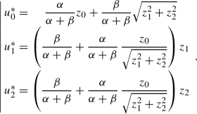
We now go back to the necessary and sufficient conditions (17). These now read as (\(u^{*}=({u_0}^{*},{u_1}^{*},{u_2}^{*})=({u_0}^{*},\overline{u^{*}})\))
Setting \(z_0=\dfrac{\dfrac{1}{\tau }\,u_0+\mu \,b_0}{\alpha }\) and \({\bar{z}}=\dfrac{\dfrac{1}{\tau }\,{\bar{u}}+\mu \,{\bar{b}}}{\beta }\) with \(\alpha =\dfrac{1}{\tau }+\mu \) and \(\beta =\dfrac{1}{\tau }+\dfrac{\mu }{2}\), these conditions amount to
We distinguish two cases:
-
Case for which \(\underline{\lambda =0:}\) Then \(\left\{ \begin{array}{c} u_0^{*}=z_0\\ \overline{u^{*}}={\bar{z}} \end{array}\right. \), with \(z_0\ge \Vert {\bar{z}}\Vert _{{\mathbb {R}}^2}\).
-
Case for which \(\underline{\lambda >0:}\)
-
Subcase \(\mathbf {z_0\ge 0}\): \(u_0^{*}=\Vert \overline{u^{*}}\Vert _{{\mathbb {R}}^2}\). \(u_0^{*}\ne 0\) otherwise \(\lambda \) would be negative. Thus, \(\overline{u^{*}}\ne 0_{{\mathbb {R}}^2}\) so that the second KKT condition in (19) reads \(\overline{u^{*}}+\frac{\lambda }{\beta }\,\frac{\overline{u^{*}}}{\Vert \overline{u^{*}}\Vert _{{\mathbb {R}}^2}}={\bar{z}}\) expressing the fact that \(\overline{u^{*}}\) and \({\bar{z}}\) are colinear with a positive coefficient. Straightforward computations give \(\overline{u^{*}}=\left( 1-\frac{\lambda }{\beta \,\Vert {\bar{z}}\Vert _{{\mathbb {R}}^2}}\right) \,{\bar{z}}\) with \(\lambda < \beta \,\Vert {\bar{z}}\Vert _{{\mathbb {R}}^2}\). At last, the first condition of (19) combined with the slackness condition (third equation of (19)) leads to
$$\begin{aligned} \lambda =\dfrac{\alpha \beta }{\alpha +\beta }\,\left( \Vert {\bar{z}}\Vert _{{\mathbb {R}}^2}-z_0\right) \end{aligned}$$with \(z_0 <\Vert {\bar{z}}\Vert _{{\mathbb {R}}^2}\) (\(\lambda < \beta \,\Vert {\bar{z}}\Vert _{{\mathbb {R}}^2}\) is ensured). Thus,
$$\begin{aligned} \left\{ \begin{array}{ccc} u_0^{*}&{}=&{}\dfrac{\alpha }{\alpha +\beta }z_0+\dfrac{\beta }{\alpha +\beta }\,\Vert {\bar{z}}\Vert _{{\mathbb {R}}^2},\\ \overline{u^{*}}&{}=&{}\left( \dfrac{\beta }{\alpha +\beta }+\dfrac{\alpha }{\alpha +\beta }\,\dfrac{z_0}{\Vert {\bar{z}}\Vert _{{\mathbb {R}}^2}}\right) {\bar{z}}. \end{array}\right. \end{aligned}$$ -
Subcase \(\mathbf {z_0< 0}:\) \(u_0^{*}=\Vert \overline{u^{*}}\Vert _{{\mathbb {R}}^2}\).
If \(\overline{u^{*}}=0_{{\mathbb {R}}^2}\), then \(u_0^{*}=0\) and \(\lambda =-\alpha \,z_0\). The second KKT condition in (19) gives \(\beta \,\Vert {\bar{z}}\Vert _{{\mathbb {R}}^2}\le -\alpha \,z_0\).
If \(\overline{u^{*}}\ne 0_{{\mathbb {R}}^2}\), again the second KKT condition in (19) shows that \(\overline{u^{*}}\) and \({\bar{z}}\) are colinear with positive coefficient \(\left( 1-\frac{\lambda }{\beta \,\Vert {\bar{z}}\Vert _{{\mathbb {R}}^2}}\right) \) so \(\lambda < \beta \,\Vert {\bar{z}}\Vert _{{\mathbb {R}}^2}\). The first condition of (19) combined with the slackness condition (third equation of (19)) leads to
$$\begin{aligned} \lambda =\dfrac{\alpha \beta }{\alpha +\beta }\,\left( \Vert {\bar{z}}\Vert _{{\mathbb {R}}^2}-z_0\right) \end{aligned}$$(\(\lambda >0\) is automatically satisfied), the constraint \(\lambda < \beta \,\Vert {\bar{z}}\Vert _{{\mathbb {R}}^2}\) reads equivalently \(\beta \,\Vert {\bar{z}}\Vert _{{\mathbb {R}}^2}>-\alpha \,z_0\) and in the end,
$$\begin{aligned} \left\{ \begin{array}{ccc} u_0^{*}&{}=&{}\dfrac{\alpha }{\alpha +\beta }z_0+\dfrac{\beta }{\alpha +\beta }\,\Vert {\bar{z}}\Vert _{{\mathbb {R}}^2},\\ \overline{u^{*}}&{}=&{}\left( \dfrac{\beta }{\alpha +\beta }+\dfrac{\alpha }{\alpha +\beta }\,\dfrac{z_0}{\Vert {\bar{z}}\Vert _{{\mathbb {R}}^2}}\right) {\bar{z}}. \end{array}\right. \end{aligned}$$
To summarize, it can be checked that:
-
If \(z_0\ge 0\)
-
(i)
If \(\Vert {\bar{z}}\Vert _{{\mathbb {R}}^2}\le z_0\), \({\text{ prox }}_{\tau \,g}(u)=(z_0,{\bar{z}})\);
-
(ii)
If \(\Vert {\bar{z}}\Vert _{{\mathbb {R}}^2}>z_0\),
$$\begin{aligned}{} & {} {\text{ prox }}_{\tau \,g}(u)=\left( \dfrac{\alpha }{\alpha +\beta }z_0 \right. \\{} & {} \quad \left. +\dfrac{\beta }{\alpha +\beta }\,\Vert {\bar{z}}\Vert _{{\mathbb {R}}^2},\left( \dfrac{\beta }{\alpha +\beta }+\dfrac{\alpha }{\alpha +\beta }\,\dfrac{z_0}{\Vert {\bar{z}}\Vert _{{\mathbb {R}}^2}}\right) {\bar{z}}\right) ; \end{aligned}$$
-
(i)
-
If \(z_0< 0\)
-
(i)
If \(\beta \,\Vert {\bar{z}}\Vert _{{\mathbb {R}}^2}\le -\alpha \,z_0\), \({\text{ prox }}_{\tau \,g}(u)=(0,0_{{\mathbb {R}}^2})\);
-
(ii)
If \(\beta \,\Vert {\bar{z}}\Vert _{{\mathbb {R}}^2}>-\alpha \,z_0\),
$$\begin{aligned}{} & {} {\text{ prox }}_{\tau \,g}(u)=\left( \dfrac{\alpha }{\alpha +\beta }z_0 \right. \\{} & {} \quad \left. +\dfrac{\beta }{\alpha +\beta }\,\Vert {\bar{z}}\Vert _{{\mathbb {R}}^2},\left( \dfrac{\beta }{\alpha +\beta }+\dfrac{\alpha }{\alpha +\beta }\,\dfrac{z_0}{\Vert {\bar{z}}\Vert _{{\mathbb {R}}^2}}\right) {\bar{z}}\right) . \end{aligned}$$
-
(i)
Remark 3
An alternative technique based on the orthogonal projection onto epigraphs can be provided to obtain the expression of \({\text{ prox }}_{\tau \,g}(u)\). This can be found in Appendix C.
According to Remark 2, convergence is ensured if \(\theta =1\) and \(\tau \sigma \Vert \nabla \Vert ^2< 1\). Since \(\Vert {\text{ div }}\Vert =\Vert \nabla \Vert \) ([26, Chapter IV, Sect. 5, Theorem 6]) and due to the previous estimate on \(\Vert {\text{ div }}\Vert \), convergence is thus guaranteed as soon as \(\tau \sigma <\frac{1}{8}\).
5 Validation
5.1 Experimental Results
To achieve the validation of the proposed theory on real Stokes images, experiments are conducted on intensity images acquired from a polarimetric camera. Note that the data that support the findings of this study are not openly available but are available from the corresponding author upon reasonable request. In our experiments, the trioptics polar4D camera is used, providing four images \(I_{0}, I_{45}, I_{90}\) and \(I_{135}\). The Stokes images are calculated both with the classical least square method (LS) and with the proposed one. The question of assessing the validity of the proposed model over the classical least square-based one encompasses several levels of discussion. Indeed, the presented experiments are intended to quantify both the relevancy of the regularization and the compliance of the recovered Stokes vectors with the physical admissibility criterion as well as sensitivity to noise. To achieve this goal and in addition to visual inspection, two metrics that encode those aspects are assessed: on the one hand, the monitoring of the DOLP for the physical admissibility verification, and on the other hand, the control of the AOLP for the physical consistency of the scene. As previously stressed, the DOLP lies between zero and one, whilst the AOLP should be homogeneous on objects made of the same material. The Stokes images calculated with the least square method as usually done in the literature are compared to those computed using the proposed solution. More precisely, to demonstrate the validity/relevance of the regularization and its influence on the AOLP over the classical least square method (LS), three configurations are considered when relevant: (i) the pure geometrical model without regularization named Geometrical Model Alone (GMA) in which the TV regularization has been removed, thus consisting of the classical \(L^2\)-penalization coupled with the geometrical constraints, (ii) the model with decoupled regularization on each channel referred to as Decoupled Model (DM) in which total variation regularization is applied independently on each channel, and (iii) our Coupled Model (CM). By saying ‘when relevant’, we mean when LS produces DOLP values strictly greater than 1, otherwise we restrict ourselves to a mere comparison between LS and CM since in this case, the physical admissibility constraints will not be active in GMA.
Extensive experiments conducted to discriminate between DM and CM show the preeminence of CM over DM, both in terms of quantitative criteria such as the AOLP and DOLP, and qualitative assessment (spatial regularization/coherency, more refined details). Thus in the presentation, we limit ourselves to the comparisons of the LS method, GMA and CM, the latter model being the one detailed in the paper. The best solution is the one achieving a DOLP between 0 and 1, while exhibiting a piecewise homogeneous AOLP. The first condition related to the DOLP (\({{S_0}} \ge \sqrt{{{S_1}}^2+{{S_2}}^2}\)) reflects the fact that the total energy of the light wave \({{S_0}} ^2\) is always greater than the energy of the deterministic part of that wave, \({{S_1}} ^2 +{{S_2}} ^2\), whereas the condition on AOLP translates the fact that two spatially close identical objects should mainly reflect the light in the same direction. The experiments are split into two sets of images: simple indoor images containing object/background and real outdoor images with non-controlled light.

First row: synthetic clean radiance images, from left to right \(I_0^{gt},I_{90}^{gt},I_{45}^{gt},I_{135}^{gt}\). Second row: their counterpart degraded by a white additive Gaussian noise with \(\sigma ^2=0.02\). Third row: recovered radiance images \(I^{*}\) obtained by computing \(AS^{*}\). The PSNR between the noise-free radiance images \(I^{gt}\) and the estimated ones \(I^{*}\) is 37.36
5.1.1 Experiments on Synthetic Data and Indoor Images
In order to substantiate the relevancy of the proposed approach, simulations on synthetic data for which ground truth is known have been performed. The artificial data have been generated based on an earlier code by Dr. Sylvain Faisan (ICube - MIV, Université de Strasbourg) dedicated to the reconstruction of full Stokes vectors [10] and that we adapted to our setting. We synthesized a 256\(\times \)256 pixel Stokes image \(S^{gt}=[S_0^{gt},S_1^{gt},S_2^{gt}]\) composed of two distinct regions: (i) a background with a uniform polarization signature \(S^{gt}=[1,\frac{1}{\sqrt{2}},\frac{1}{\sqrt{2}}]\) (totally polarized light), and (ii) a circle of radius 100 pixels with a smoothly varying partially polarized Stokes signature. The associated radiance images \(I^{gt}=[I_0^{gt},I_{90}^{gt},I_{45}^{gt},I_{135}^{gt}]\) are computed (\(I^{gt}=AS^{gt}\)) and are then degraded by an additive white Gaussian noise of variance \(\sigma ^2=0.02\). These are depicted in Fig. 3 (both clean radiance images and degraded counterparts). The initial set of data is shown in Fig. 3 second row, while the reconstructed Stokes vectors are displayed in Fig. 4 second row, the tuning parameters being set, respectively, to \(\sigma =0.3\) (Chambolle–Pock algorithm), \(\gamma =1\), \(\theta =0.5\) and \(\mu =1.5\). Visually, the reconstruction is smooth and spatially consistent, emphasizing the benefit of total variation regularization and obeys the admissibility constraint criterion, the DOLP being an element of [0, 1] (see Fig. 5). As the ground truth is known, these elements can be corroborated by the accuracy assessment, by comparing the estimated values \(S^{*}\) with the original ones \(S^{gt}\) through the formula (see again [10])
with P the number of pixels and \(\Vert \cdot \Vert \) denoting the Euclidean norm in \({\mathbb {R}}^3\). In our experiment, the Stokes vector estimation error is \({\mathcal {E}}(S^{gt},S^{*})=2.79\). Note that if the Total Variation regularization proves to be relevant in removing noise while preserving sharp edges, one of its limitations is the contrast loss (see [27]). To circumvent this issue in future works, several lines of research could be considered among which: sequential pipelines with a posteriori contrast enhancement while still preserving the physical admissibility constraint (histogram equalization, gray-scale transformation algorithms, PDE-based methods, etc.) or joint frameworks including new fidelity terms.

First row: ground truth Stokes vector \(S^{gt}=[S_0^{gt},S_1^{gt},S_2^{gt}]\). Second row: estimated Stokes vector \(S^{*}\)

Left: ground truth DOLP computed from \(S^{gt}\). Right: DOLP computed from the estimated Stokes vector \(S^{*}\)
In a second configuration, experiments are conducted on real indoor images with a few objects on a unified background. In order to avoid strong reflections focused on areas where the light source is shining, acquisitions are carried out under uniform illumination, during the day and without any artificial illumination. The protocol is illustrated on an acquisition example in Fig. 6.
The objective of this first cohort of experiments is to demonstrate, on simple object images, the quality of the recovered AOLP without any parasitic incident illumination as well as the homogeneity of the Stokes components. The media of the pot as well as the plant are not reflective, which avoids any disturbing specular reflection. Figure 7 displays the three polarization channels \({{S_0}}\), \({{S_1}}\) and \({{S_2}}\) of a plant in its pot obtained, respectively, with CM constrained by \(\sigma =0.1\) (Chambolle–Pock algorithm), \(\gamma =1\), \(\theta =0.5\) and \(\mu =20\), LS and GMA, while Fig. 8 depicts the AOLP and DOLP metrics in each case. Components \(S_1\) and \(S_2\) produced by CM are smoother than those obtained with LS and GMA, highlighting the benefit of TV regularization whilst preserving significant information. As for the DOLP, although visually similar, the ranges are not the same and in particular, the DOLP exceeds 1 at some pixels with the LS method. Those pixels having a \({\text{ DOLP }}>1\) are not physically admissible. In comparison, the DOLP calculated with the proposed method, with or without (CM/GMA) regularization, is always between 0 and 1 for each pixel, due to the exact geometrical constraint enforcement. It is worth reminding the reader that the non-compliance of some pixels with the physical constraint leads gradually to an erroneous reflection from the pixel and then to an irrelevant estimation of the object surface properties represented by the corresponding Stokes vectors. In that case, there is even no guarantee that the estimated Stokes vectors of pixels fulfilling the physical admissibility criterion are pertinent. This way of calculating the Stokes vectors is potentially wrong, showing the superiority of the proposed solution that not only respects the physical constraints of the polarization formalism but ensures homogeneity of the AOLP as will be seen next.

The experimental protocol

Row 1: three-dimensional Stokes images \({{S_0}}\), \({{S_1}}\), \({{S_2}}\) of a plant in its pot reconstructed with CM. Row 2: three-dimensional Stokes images \({{S_0}}\), \({{S_1}}\), \({{S_2}}\) of a plant in its pot reconstructed with LS. Row 3: three-dimensional Stokes images \({{S_0}}\), \({{S_1}}\), \({{S_2}}\) of a plant in its pot reconstructed with GMA

Row 1: DOLP according to LS method (left), GMA (middle) and CM (right) with colorbar. Row 2: AOLP according to LS method (left), GMA (middle) and CM (right) with colorbar

Corrupted radiance images
The second metric that has been considered here is the AOLP. When the classical least square-based method is applied, the AOLP seems to be corrupted by randomly distributed points, whereas it should be comparable for an object made of the same material. This issue is always present in the AOLP estimation and is, most of the time, a direct consequence of the non-compliance of some pixels with the physical admissibility constraint, even if it affects only a few of them. The AOLP is better represented with the proposed CM model. In this case, the AOLP is smoother, more homogeneous for an area made of the same material, especially in the regions where the incident light is uniform.
In order to substantiate even better the interest of the proposed model that handles both the issue of physical admissibility and spatial consistency, the acquired raw images from the polarimetric camera are degraded by an additive white Gaussian noise of zero mean and with variance \(\sigma ^2=0.25\). Without loss of generality and to evaluate the sensitivity of the LS method, this perturbation is applied only on one of the intensity channels arbitrarily chosen to be \(I_{45}\) in that case, that is then normalized between 0 and 1. These are displayed in Fig. 9, while the reconstructed Stokes components \(S_{0}\), \(S_{1}\), \(S_{2}\) with CM constrained by \(\sigma =0.3\) (Chambolle–Pock algorithm), \(\gamma =1\), \(\theta =0.5\) and \(\mu =4\) are depicted in Fig. 10, jointly with those obtained by LS and GMA.

Row 1: three-dimensional Stokes images \({{S_0}}\), \({{S_1}}\), \({{S_2}}\) from corrupted radiance data reconstructed with CM. Row 2: three-dimensional Stokes images \({{S_0}}\), \({{S_1}}\), \({{S_2}}\) from corrupted radiance data reconstructed with LS. Row 3: three-dimensional Stokes images \({{S_0}}\), \({{S_1}}\), \({{S_2}}\) from corrupted radiance data reconstructed with GMA

Row 1: DOLP according to LS method (left), GMA (middle) and CM (right). Row 2: AOLP according to LS method (left), GMA (middle) and CM (right)
The DOLP and AOLP are illustrated in Fig. 11 for each method. Table 1 lists the DOLP mean of the noise-free images and the one of the degraded images, together with the respective standard deviations to measure the amount of dispersion. The different figure contents correlated with the table elements express clearly the relevance of the proposed method to preserve the admissibility of polarimetric images even in noisy acquisitions and in rendering a smooth AOLP map. Moreover, when considering the DOLP calculated with the three methods, it is clear that CM is the one giving the smoother one, emphasizing the ability of the model to handle data corrupted by noise. Slightly smaller standard deviations are obtained in the case of the CM method (noisy and noise-free frameworks), reflecting a smaller dispersion of the DOLP. The significance of the proposed method is also corroborated by the images of the AOLP. Once again, the AOLP of CM is more homogeneous and is more successful in highlighting the homogeneous reflections when dealing with the same material. This analysis is finally substantiated by the recovered radiance components \(I=AS\) with S the recovered Stokes vectors by CM (Fig. 12), with in particular an estimated \(I_{45}\) component that exhibits less noise.
5.1.2 Experiments on Outdoor Polarimetric Images
For the second part of our experiments, the proposed method is evaluated on outdoor scenes with highly reflective objects, uncontrolled heterogeneous incident lights and several objects of different nature. Figure 13 displays the reconstructed Stokes components with CM constrained by \(\sigma =0.1\) (Chambolle–Pock algorithm), \(\gamma =1\), \(\theta =0.5\) and \(\mu =35\), while Fig. 14 emphasizes the results obtained for the DOLP and AOLP with the three methods.
Again, the DOLP with the proposed solution is physically admissible for the whole pixels of the image while for the least square-based model, it is greater than 1 for around \(5\%\) of the pixels. As for the AOLP, the proposed method clearly outperforms the classical one, providing a smooth consistent map. For the least square-based method, the map is corrupted by points, meaning that the reflection is strong for these pixels. This phenomenon is physically irrelevant since neighbouring pixels lying on a same material should almost have the same reflection, i.e. the same AOLP. As in indoor scenes, this issue occurs because of the non-physical admissibility of the Stokes vectors of some pixels. This problem is amplified for the AOLP estimation. In the coupled regularization model, the AOLP is much better. The reflection in homogeneous areas is roughly the same. Nevertheless, some areas exhibit a high AOLP which indicates a strong reflection: this occurs in regions where the sun is directly shining. As these areas are localized and not largely spread in the image unlike the least square-based solution, an idea to overcome this problem would be to combine the proposed solution with methods aiming to mitigate specular reflection as presented in [28] or with solutions relying on inpainting to recover the lost part of the AOLP [29]. This is, however, beyond the scope of the proposed work, the problem being independent of the physical admissibility of the Stokes vectors.

Reconstructed radiance images by CM

Row 1: three-dimensional Stokes images \({{S_0}}\), \({{S_1}}\), \({{S_2}}\) of an outdoor scene reconstructed with CM. Row 2: three-dimensional Stokes images \({{S_0}}\), \({{S_1}}\), \({{S_2}}\) of an outdoor scene reconstructed with LS. Row 3: three-dimensional Stokes images \({{S_0}}\), \({{S_1}}\), \({{S_2}}\) of an outdoor scene reconstructed with GMA

Row 1: DOLP according to LS method (left), GMA (middle) and CM (right) for the outdoor scene. Row 2: AOLP according to LS method (left), GMA (middle) and CM (right) for the outdoor scene
The last but not least experiment focuses on complicated outdoor scenes with reduced visibility and poor weather conditions such as heavy fog or snow (see Fig. 15). Recent researches claim that an excellent alternative solution for analysing such complicated images is polarimetric vision, where classical RGB images fail to overcome the drawback of low visibility, resulting in a drop of performances. This can be explained by the fact that an object reflects light even when the visibility is altered. The results of the estimated Stokes vectors with CM constrained by \(\sigma =0.1\) (Chambolle–Pock algorithm), \(\gamma =1\), \(\theta =0.5\) and \(\mu =55\) as well as the polarization characteristics are shown in Figs. 16 and 17, respectively. Note that the LS method produces DOLP values that are lower than 1 so we restrict ourselves to a strict comparison between CM and LS. This experiment thus aims to support again the fact that coupled TV regularization improves the results. As in all the previous cases, the proposed CM outperforms the classical LS. The AOLP is still not perfect in that case, but one can see much better reflection from distant objects, meaning that the estimated Stokes vectors are more representative of the physical content of the scene (see for instance [30]).

Image of a road scene under heavy fog
6 Discussion and Conclusion
This paper shows that a unique solution to the polarization optimization problem can be designed, encoding both the compliance with the physical admissibility constraints and homogeneity/regularity properties, and overcoming thus the limits of the classical least square-based method that is prone to errors. In this latter case, even if these miscalculations might only affect a small amount of pixels, they lead to an inaccurate physical representation and interpretation of the scene.
Polarization modality is able to characterize an object by multiple physical properties including its intensity, its reflection, its surface nature and roughness, and other induced physical properties such as the DOLP and the AOLP which reflect the magnitude and the direction of the reflection. As most computer vision applications rely on the quantity of information extracted from a scene, it makes polarization modality the best alternative for applications where the classical RGB modality fails. The relevance of the information given by polarization relies first on the correctness of the computed Stokes vectors, crux point of the interpretation of the scene physical content.

Row 1: three-dimensional Stokes images \({{S_0}}\), \({{S_1}}\), \({{S_2}}\) of an outdoor scene under heavy fog reconstructed with CM. Row 2: three-dimensional Stokes images \({{S_0}}\), \({{S_1}}\), \({{S_2}}\) of an outdoor scene under heavy fog reconstructed with LS

Row 1: DOLP according to LS method (left) and CM (right) for the outdoor scene under heavy fog. Row 2: AOLP according to LS method (left) and CM (right) for the outdoor scene under heavy fog
We emphasize that the correctness and suitability of the computed Stokes vectors is the primary contribution of our work. Even if the AOLP is still not perfect in the presence of noise, namely in Fig. 11 where noise is deliberately added or in Fig. 17 in the presence of heavy fog and snow, we are nevertheless ensured that, with the proposed solution, the issue does not stem from the non-respect of the physical admissibility constraint, which is essential when dealing with polarization modality. This problem could be addressed in the future by including some pre-processing steps in the pipeline to mitigate the noise affecting acquisitions or to enhance the visibility in the intensity channels before transforming them into Stokes channels. Thus, the restoration phase would be upstream, on the radiance images, and not a posteriori as in the proposed work.. These first results are cornerstone steps for further processing tasks such as segmentation, classification, detection or more generally, applications requiring a metric or a distance computed directly on Stokes images. So far, for such applications, only the intensity images \((I_0, I_{90}, I_{45}, I_{135}) \) have been utilized as complementary information when dealing with polarization-encoded images. Some works, taking advantage of the AOLP and DOLP metrics, are emerging, e.g. shape from polarization [31], transparent object normal estimation [5], showing that this field of research is thriving, enclosing a lot of interesting scientific trails, in particular in computation imaging and graphical display community. Yet, generally, Stokes vectors as well as AOLP and DOLP are most often used to visualize details difficult to see in classical images, such as transparent objects or objects exhibiting specular reflection caused by frontal sunlight. Polarization is also used for scene enhancing, where classical modality fails, such as image dehazing, depth estimation [32, 33] or to characterize the dependency of the scene on the illumination conditions [30]. We believe that the proposed work could pave the way to more involved analyses of the Stokes vectors. Indeed, up to now in the literature, no quantitative study entailing the Stokes vectors or a physical combination of them has been introduced. The main reason comes from the mathematical shape of the Stokes vectors: they do not lie in a vector space owing to the physical admissibility constraint. It is therefore inaccurate to use the Euclidean distance to compare pixels represented by two Stokes vectors. Also, two spatially close pixels may lie on different materials. The problem of comparing Stokes vectors is an ill-posed one in polarization formalism and represents a real disability to leverage the pure physical part of the polarization (Stokes vectors, AOLP, DOLP). This is a line of research we will investigate in future works by, for instance, projecting the Stokes vectors into the Minkowski space or the Krein space. However, before dealing with this pointed issue, a correct estimation of the Stokes parameters is paramount and this is what we have accomplished in this paper.
References
Wolff, L.B., Andreou, A.G.: Polarization camera sensors. Image Vis. Comput. 13(6), 497–510 (1995)
Berger, K., Voorhies, R., Matthies, L.H.: Depth from stereo polarization in specular scenes for urban robotics. In: 2017 IEEE International Conference on Robotics and Automation (ICRA), pp. 1966–1973 (2017)
Zhu, D., Smith, W.A.P.: Depth From a Polarisation + RGB Stereo Pair. In: 2019 IEEE/CVF Conference on Computer Vision and Pattern Recognition (CVPR), pp. 7578–7587 (2019)
Morel, O., Stolz, C., Meriaudeau, F., Gorria, P.: Active lighting applied to three-dimensional reconstruction of specular metallic surfaces by polarization imaging. Appl. Opt. 45(17), 4062–4068 (2006)
Miyazaki, D., Saito, M., Sato, Y., Ikeuchi, K.: Determining surface orientations of transparent objects based on polarization degrees in visible and infrared wavelengths. J. Opt. Soc. Am. A 19(4), 687–694 (2002)
Rehbinder, J., Haddad, H., Deby, S., Teig, B., Nazac, A., Novikova, T., Pierangelo, A., Moreau, F.: Ex vivo Mueller polarimetric imaging of the uterine cervix: a first statistical evaluation. J. Biomed. Opt. 21(7), 1–8 (2016)
Wang, F., Ainouz, S., Meriaudeau, F., Bensrhair, A.: Polarization-based car detection. In: 2018 25th IEEE International Conference on Image Processing (ICIP), pp. 3069–3073 (2018)
Aycock, T.M., Chenault, D.B., Hanks, J.B., Harchanko, J.S.: Polarization-based mapping and perception method and system. Google Patents. US Patent 9,589,195 (2017)
Blin, R., Ainouz, S., Canu, S., Meriaudeau, F.: Road scenes analysis in adverse weather conditions by polarization-encoded images and adapted deep learning. In: 2019 IEEE Intelligent Transportation Systems Conference (ITSC), pp. 27–32 (2019)
Faisan, S., Heinrich, C., Rousseau, F., Lallement, A., Zallat, J.: Joint filtering estimation of Stokes vector images based on a nonlocal means approach. J. Opt. Soc. Am. A 29(9), 2028–2037 (2012)
Zallat, J., Heinrich, C.: Polarimetric data reduction: a Bayesian approach. Opt. Express 15(1), 83–96 (2007)
Zallat, J., Heinrich, C., Petremand, M.: A Bayesian approach for polarimetric data reduction: the Mueller imaging case. Opt. Express 16(10), 7119–7133 (2008)
Valenzuela, J.R., Fessler, J.A.: Joint reconstruction of Stokes images from polarimetric measurements. J. Opt. Soc. Am. A 26(4), 962–968 (2009)
Chambolle, A., Pock, T.: A first-order primal-dual algorithm for convex problems with applications to imaging. J. Math. Imaging Vis. 40(1), 120–145 (2011)
Bass, M., Van Stryland, E.W., Williams, D.R., Wolfe, W.L.: Handbook of Optics, Third Edition Volume II: Design, Fabrication and Testing, Sources and Detectors, Radiometry and Photometry, 3rd edn. McGraw-Hill, Inc., New York (2009)
Terrier, P., Devlaminck, V.: Robust and accurate estimate of the orientation of partially polarized light from a camera sensor. Appl. Opt. 40(29), 5233–5239 (2001)
Ainouz, S., Morel, O., Fofi, D., Mosaddegh, S., Bensrhair, A.: Adaptive processing of catadioptric images using polarization imaging: towards a pola-catadioptric model. Opt. Eng. 52(3), 1–9 (2013)
Zubko, E., Chornaya, E.: On the ambiguous definition of the degree of linear polarization. Res. Notes AAS 3(3), 45 (2019)
Wang, Z., Zheng, Y., Chuang, Y.-Y.: Polarimetric camera calibration using an LCD monitor. In: 2019 IEEE/CVF Conference on Computer Vision and Pattern Recognition (CVPR), pp. 3738–3747 (2019)
Chambolle, A.: An algorithm for total variation minimization and applications. J. Math. Imaging Vis. 20(1), 89–97 (2004)
Pierre, F., Aujol, J.-F., Bugeau, A., Papadakis, N., Ta, V.-T.: Luminance-chrominance model for image colorization. SIAM J. Imaging Sci. 8(1), 536–563 (2015)
Azé, D.: Éléments d’analyse convexe et variationnelle. Mathématiques pour le \(2^{{\grave{{\rm e}}{{\rm me}}}}\) cycle. Ellipses, Paris (1997)
Ekeland, I., Témam, R.: Convex Analysis and Variational Problems. Society for Industrial and Applied Mathematics, Philadelphia (1999)
Moreau, J.-J.: Fonctions convexes duales et points proximaux dans un espace hilbertien. C. R. Acad. Sci. 255, 2897–2899 (1962)
Combettes, P.L., Pesquet, J.-C.: Proximal splitting methods in signal processing. In: Bauschke, H.H., Burachik, R.S., Combettes, P.L., Elser, V., Luke, D.R., Wolkowicz, H. (eds.) Fixed-Point Algorithms for Inverse Problems in Science and Engineering, pp. 185–212. Springer, New York (2011)
Kolmogorov, A., Fomine, S.: Éléments de la Théorie des Fonctions et de l’Analyse Fonctionnelle, 2nd edn. Mir, Moscow (1977)
Tang, L., Fang, Z.: Edge and contrast preserving in total variation image denoising. EURASIP J. Adv. Signal Process. 2016, 1–21 (2016)
Wang, F., Ainouz, S., Petitjean, C., Bensrhair, A.: Specularity removal: a global energy minimization approach based on polarization imaging. Comput. Vis. Image Underst. 158, 31–39 (2017)
Wang, Y., Jiang, Z., Shi, J.: Highlight area inpainting guided by illumination model. In: Fifth International Conference on Graphic and Image Processing (ICGIP 2013), vol. 9069, p. 90691 (2014). International Society for Optics and Photonics
Kupinski, M.K., Bradley, C.L., Diner, D.J., Xu, F., Chipman, R.A.: Angle of linear polarization images of outdoor scenes. Opt. Eng. 58(8), 082419 (2019)
Baek, S.-H., Jeon, D.S., Tong, X., Kim, M.H.: Simultaneous acquisition of polarimetric SVBRDF and normals. ACM Trans. Graph. 37(6) (2018)
Schechner, Y.Y., Narasimhan, S.G., Nayar, S.K.: Polarization-based vision through haze. Appl. Opt. 42(3), 511–525 (2003)
Sarafraz, A., Negahdaripour, S., Schechner, Y.Y.: Enhancing images in scattering media utilizing stereovision and polarization. In: 2009 Workshop on Applications of Computer Vision (WACV), pp. 1–8 (2009). IEEE
Beck, A.: First-Order Methods in Optimization. Society for Industrial and Applied Mathematics, Philadelphia (2017)
Acknowledgements
This project was co-financed by the European Union with the European regional development fund (ERDF, 18P03390/ 18E01750/18P02733), by the Haute-Normandie Régional Council via the M2SINUM project and by the French Research National Agency ANR via ICUB project ANR 17-CE 22-0011-01. The authors would like to thank Dr Sylvain Faisan (ICube - MIV, Université de Strasbourg) for providing us with the code to generate artificial data in the full Stokes recovery case.
Author information
Authors and Affiliations
Corresponding author
Additional information
Publisher's Note
Springer Nature remains neutral with regard to jurisdictional claims in published maps and institutional affiliations.
Appendices
Appendix A: Pointwise Infimum of Concave Functions
Let us denote by \(f(p)=\displaystyle {\inf _{S\in {\mathcal {K}}}}\,{\mathcal {L}}(S,p)=\displaystyle {\inf _{S\in {\mathcal {K}}}}\,{\mathcal {L}}_S(p)\). In our case, for each p the infimum is reached so that we could write equivalently \(f(p)=\displaystyle {\min _{S\in {\mathcal {K}}}}\,{\mathcal {L}}_{S}(p)\). Let us prove that f is concave.
We recall a preliminary result.
Theorem 3
Let X be a set and let \(f : X \rightarrow \bar{{\mathbb {R}}}\). The hypograph of f is defined by
A function \(f: X \rightarrow \bar{{\mathbb {R}}}\) is concave if and only if its hypograph is convex.
Coming back to our problem,
which is convex as the intersection of convex sets.
Appendix B: Pointwise Infimum of Continuous Functions
Theorem 4
Let \((X,\tau )\) be a topological space and let \(f : X \rightarrow \bar{{\mathbb {R}}}\) be a function. Function f is upper semi-continuous if \(\forall \alpha \in {\mathbb {R}}\), the set \(\left\{ x\in X\,\mid \,f(x)<\alpha \right\} \) is open.
Let us prove that \(f : p \in {\mathcal {B}} \mapsto \displaystyle {\inf _{S\in {\mathcal {K}}}}\,{\mathcal {L}}(S,p)\) is upper semi-continuous. Let \(\alpha \in {\mathbb {R}}\). Let \(p\in f^{-1}((-\infty ,\alpha ))\). Then, \(\displaystyle {\inf _{S\in {\mathcal {K}}}}\,{\mathcal {L}}(S,p)<\alpha \) and there exists \({\bar{S}}_p\in {\mathcal {K}}\) such that \({\mathcal {L}}({\bar{S}}_p,p)={\mathcal {L}}_{{\bar{S}}_p}(p)<\alpha \). This implies that
which is open as the union of open sets.
Appendix C: Alternative Proof to Get the Proximal Operator of \(\tau \, g\)
Consider the three-dimensional optimization problem
Using the identity
and the fact that \(A^TA=\begin{pmatrix}1&{}0&{}0\\ 0&{}\frac{1}{2}&{}0\\ 0&{}0&{}\frac{1}{2} \end{pmatrix}\), the minimization problem can be equivalently restated as:
with \(\left\{ \begin{array}{cccc} \alpha &{}=&{}\frac{1}{2\tau }+\frac{\mu }{2}\\ \beta &{}=&{}\frac{1}{2\tau }+\frac{\mu }{4} \end{array}\right. \), and \(z_0=\frac{\frac{1}{2\tau }u_0+\frac{\mu }{2}b_0}{\alpha }\), \(z_1=\frac{\frac{1}{2\tau }u_1+\frac{\mu }{2}b_1}{\beta }\) and \(z_2=\frac{\frac{1}{2\tau }u_2+\frac{\mu }{2}b_2}{\beta }\).
We then set \(\left\{ \begin{array}{ccc}{\bar{u}}_0&{}=&{}\sqrt{\alpha }\,{\tilde{u}}_0\\ {\bar{u}}_1&{}=&{}\sqrt{\beta }\,{\tilde{u}}_1\\ {\bar{u}}_2&{}=&{}\sqrt{\beta }\,{\tilde{u}}_2 \end{array}\right. \), \(\left\{ \begin{array}{ccc}{\bar{z}}_0&{}=&{}\sqrt{\alpha }\,z_0\\ {\bar{z}}_1&{}=&{}\sqrt{\beta }\,z_1\\ {\bar{z}}_2&{}=&{}\sqrt{\beta }\,z_2 \end{array}\right. \) and \(\overline{{\mathcal {C}}}\) the closed convex set defined by
and consider the auxiliary problem related to (C1)
which thus amounts to computing the projection of \({\bar{z}}=({\bar{z}}_0,{\bar{z}}_1,{\bar{z}}_2)\) onto \(\overline{{\mathcal {C}}}\). Once the (unique) solution of (C2) is obtained, it suffices to use the previous change of variable to recover the \(u^{*}_i\)’s.
Let us now recall the following result dedicated to orthogonal projection onto epigraphs.
Theorem 5
Orthogonal projection onto epigraphs, taken from [34, Chapter 6, Theorem 6.36] with \({\mathbb {E}}\) a Euclidean space, let
where \(g : {\mathbb {E}} \rightarrow {\mathbb {R}}\) is convex. Then,
where \(\lambda ^{*}\) is any positive root of the function
In addition, \(\Psi \) is nonincreasing.
We invoke the previous theorem with \(g(\cdot )=\sqrt{\frac{\alpha }{\beta }}\,\Vert \cdot \Vert _{{\mathbb {R}}^2}\) to obtain the formula and follow the arguments of Beck ([34, Chapter 6]) (we respect the same order in the arguments of \(P_{\overline{{\mathcal {C}}}}(\cdot )\) as in [34])
where \(\lambda ^{*}\) is any positive root of the function \(\Psi (\lambda )=\sqrt{\frac{\alpha }{\beta }}\,\Vert {\text{ prox }}_{\lambda \,\sqrt{\frac{\alpha }{\beta }}\Vert \cdot \Vert _{{\mathbb {R}}^2}}({\hat{z}})\Vert _{{\mathbb {R}}^2}-\lambda -{\bar{z}}_0\).
Let \(({\hat{z}},\bar{z_0})\) be such that \({\bar{z}}_0 <\sqrt{\frac{\alpha }{\beta }}\,\Vert {\hat{z}}\Vert _{{\mathbb {R}}^2}\).
Recall that
Plugging the above into the expression of \(\Psi \) leads to
The unique positive root \(\lambda ^{*}\) of the piecewise linear function \(\Psi \) is
resulting in

If we summarize the whole results, coming back to the initial variables, we see that we recover the results obtained with the necessary and sufficient KKT condition. Indeed,
-
If \({\bar{z}}_0 \ge \sqrt{\frac{\alpha }{\beta }}\,\Vert {\hat{z}}\Vert _{{\mathbb {R}}^2}\) or equivalently, \(z_0\ge \sqrt{z_1^2+z_2^2}\),
$$\begin{aligned}&\left( \sqrt{\alpha }u^{*}_0,\sqrt{\beta }u^{*}_1,\sqrt{\beta }u^{*}_2 \right) =({\bar{z}}_0,{\bar{z}}_1,{\bar{z}}_2)\\&\quad =\left( \sqrt{\alpha }z_0,\sqrt{\beta }z_1,\sqrt{\beta }z_2\right) , \end{aligned}$$yielding
$$\begin{aligned} \left( u^{*}_0,u^{*}_1,u^{*}_2 \right) =(z_0,z_1,z_2). \end{aligned}$$ -
If \({\bar{z}}_0 <\sqrt{\frac{\alpha }{\beta }}\,\Vert {\hat{z}}\Vert _{{\mathbb {R}}^2}\) or equivalently, \(z_0< \sqrt{z_1^2+z_2^2}\),
-
(i)
If \({\bar{z}}_0 \ge 0\) (or equivalently \(z_0\ge 0\)), then \(\Vert {\hat{z}}\Vert _{{\mathbb {R}}^2}\ge -{\bar{z}}_0\sqrt{\frac{\alpha }{\beta }}\) or equivalently \(\beta \,\sqrt{z_1^2+z_2^2}\ge -\alpha \,z_0\), and intermediate computations lead to
-
(ii)
If \({\bar{z}}_0<0\) (or equivalently, \(z_0<0\)) and \(\Vert {\hat{z}}\Vert _{{\mathbb {R}}^2}<-{\bar{z}}_0\sqrt{\frac{\alpha }{\beta }}\) or equivalently \(\beta \,\sqrt{z_1^2+z_2^2}< -\alpha \,z_0\), then
$$\begin{aligned} \left( u^{*}_0,u^{*}_1,u^{*}_2 \right) =(0,0,0). \end{aligned}$$ -
(iii)
If \({\bar{z}}_0<0\) (or equivalently, \(z_0<0\)) and \(\Vert {\hat{z}}\Vert _{{\mathbb {R}}^2}\ge -{\bar{z}}_0\sqrt{\frac{\alpha }{\beta }}\) or equivalently \(\beta \,\sqrt{z_1^2+z_2^2}\ge -\alpha \,z_0\), then intermediate computations lead to


Rights and permissions
Springer Nature or its licensor (e.g. a society or other partner) holds exclusive rights to this article under a publishing agreement with the author(s) or other rightsholder(s); author self-archiving of the accepted manuscript version of this article is solely governed by the terms of such publishing agreement and applicable law.
About this article

Cite this article
Le Guyader, C., Ainouz, S. & Canu, S. A Physically Admissible Stokes Vector Reconstruction in Linear Polarimetric Imaging. J Math Imaging Vis 65, 592–617 (2023). https://doi.org/10.1007/s10851-022-01139-2
Received:
Accepted:
Published:
Issue Date:
DOI: https://doi.org/10.1007/s10851-022-01139-2