
Abstract
Cooper storage is a widespread technique for associating sentences with their meanings, used (sometimes implicitly) in diverse linguistic and computational linguistic traditions. This paper encodes the data structures and operations of cooper storage in the simply typed linear \(\lambda \)-calculus, revealing the rich categorical structure of a graded applicative functor. In the case of finite cooper storage, which corresponds to ideas in current transformational approaches to syntax, the semantic interpretation function can be given as a linear homomorphism acting on a regular set of trees, and thus generation can be done in polynomial time.
1 Introduction
Since Montague (1973), a guiding principle in the semantics of natural language has been to map sentences to meanings homomorphically based on their syntactic structure. The proper treatment of quantification has been challenging from the outset, as quantifier denoting expressions seem in general to be structurally embedded inside of the expressions whose meanings they should take as their arguments. The strategy of Montague (1973), adopted by much of the subsequent linguistic literature, is to change the structures of syntax so as to have the quantificational elements in as transparent a position as possible for semantic interpretation.
Cooper storage (Cooper 1983) is a technique for interpreting sentences with quantificational elements based on structures where these elements are not in the positions which straightforwardly correspond to their semantic scopes. It involves assigning to each node of a syntax tree, in a non-deterministic recursive bottom-up manner, a pair consisting of an expression in some logical language with variables which will here be called the main expression, and a data structure, called the store, containing pairs of a free variable and a logical expression. The main expression associated with a node indicates the intended meaning of the syntax tree rooted at that node, whereas the store contains expressions representing the meanings of parts of the syntax tree rooted at that node whose relative scope with respect to the entire syntax tree have yet to be determined.
The main formal problem surrounding cooper storage is that it requires some mechanism for avoiding accidental variable capture (Sect. 1.2), and thus, among other things, this means that the map from parse tree to meaning cannot be represented as a \(\lambda \)-homomorphism (de Groote 2001a). This makes difficult an understanding of the complexity of the form-meaning relation expressed by grammars making use of cooper storage.
This paper
-
provides a general characterization of cooper storage in terms of graded applicative functors. This characterization has as special cases the variations on the cooper storage theme present in the literature.
-
provides a sequent notation for cooper storage. As this notation is very close to that of Cooper (1983), it can be viewed as putting this latter on solid logical ground.
-
interprets cooper storage in the linear lambda calculus. This makes available access to general complexity theoretic results in particular on parsing and generation (Kanazawa 2017).
From a type-logical perspective, cooper storage seems like the mirror image of hypothetical reasoning; instead of using hypotheses to saturate predicates, and only introducing quantified expressions in their scope positions, predicates are directly saturated with quantified expressions. This situation, while logically somewhat backwards, allows the otherwise higher order proof structures to be simulated with simpler second order terms (i.e. trees).
From a transformational, LF-interpretation based, perspective, it is intuitive to think of the main expression as the meaning of the LF-tree rooted in that node, with variables for traces, and of the store as containing the meanings of the quantifiers which have not yet reached their final landing site (Larson 1985). Indeed, recent proposals about compositional semantics in minimalist grammars (Kobele 2006, 2012; Hunter 2010) implement quantifier-raising using cooper storage. These approaches exploit the ‘logical backwardness’ (as described above) of cooper storage to account for empirical constraints on scope possibilities in natural language.
1.1 Examples
Two case studies in cooper storage are developed here which will be returned to throughout this paper. The first (in Sect. 1.1.1) is an instance of a traditional perspective on cooper storage; cooper storage is used to interpret a context-free grammar for a naıve fragment of English. It is included here to fix notation, as well as to provide intuitions for the rationale of cooper storage. The second (in Sect. 1.1.2) uses cooper storage to interpret movement (and reconstruction), as in the literature on minimalist syntax and semantics (Kobele 2006). It is included so as to provide a nonstandard use of cooper storage, which the resulting formalism should be able to account for.
The case studies make use of grammar formalisms of different formal power [context-free grammars, and multiple context-free grammars (Seki et al. 1991)]. In order to minimize the notational distance between the examples, I will make use of the formalism of (second order) abstract categorial grammars (ACGs) (de Groote 2001a), in particular the bottom-up Horn clause notation of Kanazawa (2009). A second order ACG consists of a context-free grammar specifying well-formed derivation trees, along with a means of homomorphically interpreting these structures.
A context-free production of the form \(X \rightarrow Y_1 \dots Y_n\) is written instead as  . The left hand side of such a clause is called the head of the clause,Footnote 1 and the right hand side of a clause is called its body. In general, a clause is of the form
  , where \(y_1,\dots ,y_n\) are variables, and M is a term whose free variables are among \(y_1,\dots ,y_n\). Clauses are naturally read in a bottom-up manner, with the interpretation that expressions \(y_1,\dots ,y_n\), of categories \(Y_1,\dots ,Y_n\) respectively, can be used to construct an expression of category X by combining them in the way specified. This can be presented succinctly in terms of an inference system, deriving judgments of the form \(\vdash X(M)\), asserting that M is an object of type X. The rules of such an inference system are given by the clauses, with the atoms in the body as antecedents, and the head as conclusion:
where \(M[y_1:= N_1,\ldots ,y_n:= N_n]\) represents the simultaneous substitution of each variable \(y_i\) in M with the term \(N_i\), for \(1 \le i \le n\).
Clauses can be multiply annotated, so that atoms are of the form \(\text {X}(x)(x')\). In this case, the grammar can be thought of as constructing multiple objects in parallel, e.g. a pronounced form in tandem with a semantic form.
1.1.1 Traditional Cooper Storage
Consider a linguist analysing a language (English), who for various reasons has decided to analyze the syntactic structure of a sentence like 1 as in Fig. 1.
-
1.
The reporter will praise the senator from the city.
The linguist has come up with a compositional semantic interpretation for this analysis, and the clauses are annotated with both a pronounced and a semantic component. As an example, consider the clause for \({\text {IP}}\) in the figure;  . This clause can be read as saying that an I’ pronounced t with meaning i and a DP pronounced s with meaning d can be combined to make an IP pronounced \(s^\frown t\) with meaning \(\textsc {fa}\ i\ d\) (i.e. the result of applying i to d). There is a general X-bar theoretic clause schema, allowing for unary branching (an XP can be constructed from an X’, and an X’ from an X), which is intended to stand for a larger (but finite) set of clauses, one for each category used in the grammar. The clause schema
  is intended to be read as saying that a word w has its lexically specified meaning w (and is of a lexically specified category X); a clause without any right hand side functions as a lexical item; it allows for the construction of an expression without any inputs.

A grammar and syntactic analysis of sentence 1
In Fig. 1, the expressions of category DP have been analysed as being of type e, that is, as denoting individuals.Footnote 2 While this is not an unreasonable analytical decision in this case (where the can be taken as denoting a choice function), it is untenable in the general case. Consider the linguist’s reaction upon discovering sentence 2, and concluding that determiners are in fact of type (et)(et)t (i.e. that they denote relations between sets).
-
2.
No reporter will praise a senator from every city.
The immediate problem is that the clauses constructing expressions out of DPs (those with heads \(\text {P'}(s^\frown t)(\textsc {fa}\ p\ d)\), \(\text {V'}(s^\frown t)(\textsc {fa}\ v\ d)\), and \(\text {IP}(s^\frown t)(\textsc {fa}\ i\ d)\)) are no longer well-typed; the variable d now has type (et)t and not e. While in the clause with head \(\text {IP}(s^\frown t)(\textsc {fa}\ i\ d)\) this could be remedied simply by switching the order of arguments to \(\textsc {fa}\), there is no such simple solution for the others, where the coargument is of type eet.Footnote 3

Preserving syntactic structure via cooper storage
The linguist might first investigate solutions to this problem that preserve the syntactic analysis. One diagnosis of the problem is that whereas the syntax was set up to deal with DPs of type e, they are now of type (et)t. A solution is to allow them to behave locally as though they were of type e by adding an operation (storage) which allows an expression of type (et)t to be converted into one which behaves like something of type e. This is shown in Fig. 2. This notion of ‘behaving like something’ of another type is central to this paper, and will be developed formally in Sect. 3. For now, note that the linguist’s strategy was to globally enrich meanings to include a set (a quantifier store) containing some number of variables paired with quantificational expressions. An expression now denotes a pair of the form \(\langle x,X\rangle \), where the first component, x, is of the same type as the denotation of that same expression in the grammar of Fig. 1. Inspecting the clauses in Fig. 2, one sees that all but the two labeled storage or retrieval correspond to the clauses in the previous figure. Indeed, restricting attention to just the first component of the meanings in these clauses, they are identical to those in the previous figure. The second component of an expression’s denotation is called a store, as it stores higher typed meanings until they can be appropriately integrated with a first component. An expression with meaning \(\langle x,X\rangle \) can, via the storage rule, become something with the meaning \(\langle \textsf {y},\{\langle \textsf {y},x\rangle \}\cup X\rangle \); here its original meaning, x : (et)t, has been replaced with a variable \(\textsf {y} : e\), and has been pushed into the second components of the expression’s meaning. The retrieval rule allows for a pair \(\langle \textsf {y},x\rangle \) in the second meaning component to be taken out, resulting in the generalized quantifier representation x to take as argument a function created by abstracting over the variable \(\textsf {y}\).Footnote 4 Note that, while the syntactic structure is now different, as there are multiple unary branches at the root (one for each quantifier retrieved from storage), this difference is not of the kind that syntactic argumentation is usually sensitive to. Thus, this plausibly preserves the syntactic insights of our linguist.
This example will be revisited in Figs. 13 and 14.
It is worth noting some formal aspects of this grammar which are easily overlooked. First, the syntactic grammar itself generates infinitely many structures (the rule involving retrieve is a context-free production of the form \({\text {IP}} \rightarrow {\text {IP}}\)). Most of these will not have a semantic interpretation, as retrieve is partial: one cannot retrieve from an empty store. Thus, in the general case, using cooper storage in this way to interpret even a context free grammar will result in a properly non-regular set of parse trees being semantically well-formed: if all retrieval steps are deferred to the end of the derivation (as they are in this example), then the semantically interpretable parse trees will be those which begin with a prefix of unary branches of length no more than k, where k is the number of elements which have been stored in the tree. Second, we are primarily interested in those expressions with empty stores. As expressions of indefinitely many types may be used in a given grammar, this cannot be given a finite state characterization. Finally, the retrieve operation as given is inherently non-deterministic. This non-determinism could be pushed instead into the syntax, given a more refined set of semantic operations, as will be done in the next example.
1.1.2 Movement via Cooper Storage
The previous section presented cooper storage in its traditional guise; quantificational expressions can be interpreted higher, but not lower, than the position they are pronounced in. More importantly, in the traditional presentation of cooper storage, the quantifiers in the store are completely dissociated from the syntax. Much work in linguistic semantics (particularly in the tradition of transformational generative grammar) attempts to identify constraints on the scope-taking possibilities of quantificational expressions in terms of their syntactic properties [see, e.g. Johnson (2000)]. In this tradition, nominal phrases (among others) are typically syntactically dependent on multiple positions (their deep, surface, and logical positions).
A linguist might, in order to have a simple syntactic characterization of selectional restrictions across sentences like 3 and 4, analyze there as being a single structural configuration in which the selectional restrictions between subject and verb obtain, which is present in both sentences.
-
3.
A dog must bark.
-
4.
A dog must seem to bark.
Figure 3 again uses a Horn-clause like notation, and a production has the form  . The \(\mathbf {y_i}\) on the right hand side of such a rule are finite sequences of pairwise distinct variables, and the \(\mathbf {x}\) on the left is a finite sequence consisting of exactly the variables used on the right. Instead of deriving a set of strings, a non-terminal derives a set of finite sequences of strings. Categories will in this example consist of either pairs or singletons of what are called in the transformational syntax literature feature bundles, and heavy use of polymorphism will be made (the polymorphic category \([f\alpha ,\beta ]\) is unifiable with any instantiated category of the form [fg, h], for any g and h).Footnote 5 The basic intuition behind the analysis in Fig. 3 is that a noun phrase (a dog) is first combined syntactically with its predicate (bark), and is then put into its pronounced position when this becomes available.

A transformational grammar and analysis of sentences 3 and 4

Interpreting deep structures
A straightforward semantic interpretation scheme simply maps the derivation tree homomorphically to a meaning representation, with binary branching rules corresponding to (either forward or backward) function application, and unary branching rules to the identity function, as shown in Fig. 4. Here the literals are of the form \(X(\mathbf {x})(x')\), where X and \(\mathbf {x}\) are as before, and \(x'\) is a meaning representation (on the left \(x'\) is a term, and on the right a variable). This allows the linguist to assign the meaning in 5 to sentence 3.
-
5.
It must be the case that a dog barks.


However, sentence 3 is ambiguous; another reading of this sentence is as in 6.
-
6.
There is a dog which must bark.


The linguist might be tantalized by the fact that the currently underivable reading 6 fits naturally with the surface word order, and indeed, in the derivation of sentence 3 in Fig. 3, the string a dog, although introduced before must, is prepended to it in the last step. To allow the quantificational aspect of a dog to remain active as long as its phonetic aspect is, the linguist extends meanings with a finite store, whose elements are in correspondence with the derived string parts of the expression, as shown in Fig. 5. Here the literals are of the form \(X(\mathbf {x})(\mathbf {x}')\), where the meaning component \(\mathbf {x}'\) is a sequence of meaning representations. The two readings (5 and 6) of sentence 3 are shown in Fig. 6. (Just the meaning components are shown, as the strings are identical.)

Additional rules for surface scope interpretation

Two readings of 3
This example will be revisited in Figs. 15 and 16.
In contrast to the previous example, here the size of the cooper store is finitely bounded (at 1). This means that the set of syntactically and semantically well-formed derivations is regular; only finitely many semantic types are used in this grammar, and these can be (and have been) encoded into the syntactic category information of the grammar.
1.2 Making it Compositional
As presented above, the data structures involved in cooper storage are not semantic; the objects of the theory are syntactic representations of semantic objects: free variables (or indices of variables) are used to maintain a link between the objects in the store and the semantic arguments they should bind in the main expression. It is of course possible to ‘semanticize’ variables by reifying assignment functions [as is done explicitly in the textbook of Kreisel and Krivine (1967)], and to reconceptualize variables as functions from assignment functions to individuals. Indeed, both Cooper (1983) and (much later) Kobele (2006) assign the same denotation to objects in the store. Letting g be the type of assignment functions, the representation \(\langle x_i, \left[ \left[ NP \right] \right] \rangle \) is viewed as a model-theoretic object of type (gt)gt mapping over sentence denotations dependent on a variable assignments in the following way:Footnote 6
The deeper problem is that there is no mechanism to ensure freshness of variables; each time the storage rule is used a globally unique variable name should be produced. Kobele (2006), exploiting the fact that variable names can be uniquely associated with nodes in the derivation tree (the point at which the storage rule is used), uses combinators to encode pairs of assignment functions as single assignment functions in a way that allows stored elements to correctly identify the variable they should ‘bind’. This convoluted move requires variable binding operators to be simulated via model theoretic objects (of type e.g. (gt)egt). When it seems one is reinventing well-understood machinery, it is reasonable to try to recast the problem being addressed so as to take advantage of what already exists.
The problem is that free variables are being used (either syntactically or semantically), and these necessitate a complicated sort of bookkeeping. In particular, 1. free variables appear in the main expression, and 2. stored items are paired with free variables. Given the intended use of these free variables, which is that the variable paired with a stored item be abstracted over in the main expression when this stored item is retrieved, the resolution to both of these problems is simple and in retrospect obvious: this lambda abstraction takes place immediately, and is not deferred to some later point in time. Eliminating free variables then obviates the need for fresh variables. The basic idea of this paper is:
An expression of the form \(M, \{ \langle x_1,N_1\rangle ,\ldots ,\langle x_k,N_k\rangle \}\) should instead be replaced by one of the form \(\langle \lambda x_1,\ldots ,x_k.M, N_1,\ldots ,N_k\rangle \).
Crucially, the M and \(N_i\)s in the first expression are syntactic objects (formulae in some logical language), while in the second expression they are semantic objects (whatever those may be). The intent of Cooper’s store is to have all and only those variables free in M which are paired with some expression in the store; pairing a variable with an expression in the store is simply a means to keep track of which argument position this latter expression should be binding. Thus there is a systematic relation between the type of the expressions in the original cooper store and the type of their reformulation here; roughly, if \(M,\langle x_1,N_1\rangle ,\dots ,\langle x_k,N_k\rangle \) is such that \(M : \alpha \), and for all \(1 \le i \le k\) \(x_i : \beta _i\) and \(N_i : \gamma _i\), then \(\lambda x_1,\dots ,x_k.M\) has type \(\beta _1 \mathrel {\rightarrow } \cdots \mathrel {\rightarrow } \beta _k \mathrel {\rightarrow } \alpha \), and the objects \(N'_i\) in the store have type \(\gamma _i\). Generally, there will be some systematic relation between \(\beta _i\) and \(\gamma _i\); typically \(\gamma _i\) is the type of a function taking a continuation of something of type \(\beta _i\); \(\gamma _i = (\beta _i \mathrel {\rightarrow } \eta ) \mathrel {\rightarrow } \eta \). I will call \(\beta \) the trace type of \(\gamma \), and write \(\mathtt {t}_\gamma := \beta \). The intent behind the introduction of the terminology of trace types is to abstract away from the precise relation between the type of a stored expression and the type of the variable associated with it.
All relevant information about the type of an expression cum store is therefore given by the list of types \(p := \gamma _1,\dots ,\gamma _k\) of expressions in the store, together with the result type \(\alpha \) of the main expression. The type  is the type of the main expression, and
  is the type associated with expressions cum stores with list of stored expression types p and main expression type \(\alpha \) (this will be revised in a later section).Footnote 7

While I will show that the cooper store data structure can be encoded in the lambda calculus in the above way, the crucial contribution of this paper is to observe that this type theoretic encoding reveals a non-trivial structure, that of a graded applicative functor. Thus all of the operations usually performed on cooper storage expressions are also definable in the simply typed lambda calculus, and moreover the fact that expressions with attached stores behave for most intents and purposes as though they had the type \(\alpha \) (as opposed to  ), is a consequence of this structure.
1.3 Related Work
de Groote (2001b) presents linguistic applications of the \(\lambda \mu \)-calculus of Parigot (1992).Footnote 8 In particular, the \(\lambda \mu \)-term \(\lambda P.\mu \alpha .{\texttt {every}}(P)(\lambda x.\alpha x)\), proposed as the meaning representation of the word every, has type (et)e. He notes that cooper storage can be thought of in these terms; here storage is built in to lexical meaning representations using \(\mu \)-abstraction, and the reductions for \(\mu \) behave like retrieval. In order to account for scope ambiguities, de Groote proposes to use a non-confluent reduction strategy. Crucially, \(\mu \)-reduction is completely divorced from syntactic structure [just as is retrieval in Cooper (1983)]. This means that alternative versions of cooper storage which enforce a tighter connection between syntactic operations and stored elements, as Sect. 1.1.2, are not straightforwardly implementable using the \(\lambda \mu \)-calculus.
A recent type-logical presentation of cooper storage is given in Pollard (2011). There a sequent is of the form \(\varGamma \vdash M : \alpha \dashv \varDelta \), where \(\varGamma \) is a variable context, \(\varDelta \) is a set of pairs of the form \(\langle x,N\rangle \), where x is a variable, and M and N are what Pollard calls rc-terms with free variables among those in \(\varGamma \) and \(\varDelta \) (rc-terms are not quite \(\lambda \)-terms, but are straightforwardly interpretable as such). Here, \(\varDelta \) is simply a quantifier store, exactly as in Cooper (1983); indeed Pollard (2011) is explicitly trying to give a direct type-logical implementation of cooper storage. There are two substantive differences between Pollard’s proposal and the one in this paper. First, in Pollard (2011), stored elements may contain free variables. From a more categorical perspective, an RC-sequent of the form \(\varGamma \vdash M : \alpha \dashv \varDelta \) can be thought of (being somewhat loose with notation) as a term of type  , where
  are the types of the free variables in M from \(\varDelta \). Thus a rule of hypothetical reasoning would be invalid (as variables in either of \(\varGamma \) or
  may occur in \(\varDelta \)). Indeed, no rule for implication elimination from \(\varGamma \) is proposed in Pollard (2011), and the corresponding rule for \(\varDelta \) is restricted so as to be applicable only in case the variable does not occur in any terms in \(\varDelta \). The lack of such a rule is noted in de Groote et al. (2011). The presentation here simply rebrackets so as to obtain
  . Second, Pollard uses variables to coordinate the stored expressions with the positions they should ultimately bind into. The proposal here takes advantage of the additional structure in this problem made explicit in the above categorical presentation of types to eschew variables. Namely, the expressions in the store are in a bijective correspondance with the positions they are intended to bind into, which allows this coordination to be achieved by introducing and enforcing an order invariant between the abstractions
  and the store \(\varDelta \).
These differences notwithstanding, the present paper (especially given the sequent presentation of cooper storage in Sect. 4.3) can be thought of as a continuation of the logical approach to cooper storage initiated in Pollard (2011), offering in particular an embedding of the cooper-storage proof system into the linear lambda calculus, as well as a formal specification of the underlying algebraic structures involved.
1.4 Structure of the Paper
The remainder of the paper is structured as follows. In the next section are formal preliminaries. The following section introduces the relevant category theoretic notion of applicative functors (but without category theory), defines their graded variants, and proves that they enjoy familiar formal properties. Then it is shown that the data structure underlying cooper storage is in fact a graded applicative functor, which supports the operations particular to the use of cooper storage in semantics (in particular, retrieval and storage). Various instantiations of the general cooper-storage scheme are presented, which allow for the recasting of the examples in Sects. 1.1.1 and 1.1.2 in these terms.
2 Formal Preliminaries
2.1 Partial Functions and Algebras
Given a set A, let \(\bot {}\) be a symbol not in A and define \(A_{\bot {}} = A \cup \{\bot {}\}\). A partial function with domain A and codomain B is here identified with a total function \(f : A \rightarrow B_{\bot {}}\) where f is said to be undefined on \(a \in A\) if \(f(a) = \bot {}\). I write \({\textsf {def}}(f) = f^{-1}(B)\) for the subset of elements in its domain on which f is defined, and \(\left[ A \hookrightarrow B\right] \) for the set of all partial functions from A to B. Given \(A \subseteq B\), a partial function \(f : A \hookrightarrow C\) can be coerced to one with domain B by setting \(f(b) = \bot {}\) for all \(b \in B - A\). Note that this preserves \({\textsf {def}}(f)\). The empty function is undefined on all objects in its domain. (Equivalently, it is (a coercion of) the unique map with domain \(\emptyset \).) Two partial functions \(f,g : A \hookrightarrow B\) are compatible iff \({\textsf {def}}(f) \cap {\textsf {def}}(g) = \emptyset \). Given compatible f and g, their superposition is defined to be \(f \oplus g : A \hookrightarrow B\) where \((f\oplus g)(a) = \mathbf{if }a \in {\textsf {def}}(f) \mathbf{ then }f(a)\mathbf{ else }g(a)\). Note that \(f\oplus g\) is just the set theoretic union of f and g viewed as sets of pairs.
I assume familiarity with basic notions of algebra. A monoid  consists of a set M together with a designated element
  and an associative operation
  for which
  is an identity. A monoid homomorphism between M and \(M'\) is a function \(h : M \rightarrow M'\) such that
  and
and  . A partial monoid is a monoid which contains an absorbing element \(\bot {}\) such that
  . Often the absorbing element will be left implicit (i.e. the carrier set of the partial monoid will be given as M instead of as \(M_\bot \)). Homomorphisms between partial monoids are required to in addition map absorbing elements to absorbing elements. A monoid is abelian iff
  is commutative.
Note that for any sets A, B, the set \(\left[ A\hookrightarrow B\right] \) together with \(\oplus \) and the empty function forms a partial abelian monoid.
2.2 \(\lambda \)-Calculus and Types
Here I briefly recall the simply typed \(\lambda \)-calculus (Barendregt et al. 2013). I will write typed terms in the Curry style, but will, if convenient, indicate the type of a variable in a binding construct with a superscript (e.g. \(\lambda x^\alpha .M\)).
Given a finite set A of atomic types, the set \(\mathcal {T}_A\) of (simple) types over A is the smallest superset of A such that \(\alpha ,\beta \in \mathcal {T}_A\) implies that \((\alpha \mathrel {\rightarrow } \beta )\in \mathcal {T}_A\).
As is common, parentheses are omitted whenever possible, writing \(\alpha \mathrel {\rightarrow } \beta \) for \((\alpha \mathrel {\rightarrow } \beta )\). Implication (i.e. the operator \( \mathrel {\rightarrow } \)) associates to the right; thus \(\alpha \mathrel {\rightarrow } \beta \mathrel {\rightarrow } \gamma \) stands for \(\alpha \mathrel {\rightarrow } (\beta \mathrel {\rightarrow } \gamma )\).
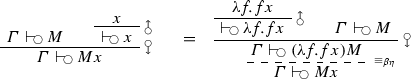
Given a countably infinite set X of variables, the set \(\varLambda \) of \(\lambda \)-terms is the smallest set containing X which is closed under application and abstraction
Parentheses are omitted under the convention that application associates to the left, i.e. MNO is ((MN)O), and multiple abstractions are written as one, i.e. \(\lambda x,y.M\) is \(\lambda x.(\lambda y.M)\). The simultaneous capture avoiding substitution of \(N_1,\dots ,N_k\) for \(x_1,\dots ,x_k\) in M is written \(M[x_1:=N_1,\dots ,x_k:=N_k]\). Terms are identified up to renaming of bound variables. The standard notions of \(\beta \) reduction and \(\eta \) expansion are as follows: \((\lambda x.M) N \Rightarrow _\beta M[x:=N]\) and, provided x is not free in M, \(M \Rightarrow _\eta \lambda x.M x\). A term M is equivalent to N, written \(M \equiv _{\beta \eta } N\) just in case M and N can be reduced to the same term O in some finite number of \(\beta \) or \(\eta \) steps. By the Church–Rosser theorem, this notion of equivalence is in fact an equivalence relation (Barendregt et al. 2013).
A term is linear just in case every \(\lambda \) abstraction binds exactly one variable (i.e. in every subterm of the form \(\lambda x.M\), x occurs free exactly once in M). An important property of linear terms (up to equivalence) is that they are uniquely determined by their principal (most general) type (Babaev and Soloviev 1982). A linear \(\lambda \)-term M has a type \(\alpha \) (when its free variables are assigned types as per a variable context \(\varGamma \)) just in case the sequent \(\varGamma \vdash M : \alpha \) can be derived using the inference rules in Fig. 7 (in the \(\rightarrow E\) rule it is assumed that the domains of \(\varGamma \) and \(\varDelta \) are disjoint, see the text below for the definition of the comma notation). A (variable) context \(\varGamma : X \hookrightarrow \mathcal {T}_A\) is a partial function such that \(\left| {\textsf {def}}(\varGamma )\right| \in \mathbb {N}\); it is defined only on a finite subset of X. A context \(\varGamma \) will be sometimes represented as a list \(x_1 : \alpha _1,\dots ,x_n : \alpha _n\), which is to be understood as indicating that \(\varGamma \) is defined only on \(x_1,\dots ,x_n\) and maps each \(x_i\) to \(\alpha _i\). If contexts \(\varGamma \) and \(\varDelta \) are compatible, I write \(\varGamma ,\varDelta \) instead of \(\varGamma \oplus \varDelta \).

Linear typing rules
3 (Graded) Applicative Functors
A fundamental intuition behind cooper storage is that the meaning of a parse tree node, while complex (of high type), behaves as though it were far simpler (of lower type). For example, whereas a predicate might intuitively denote a function of type \(e \rightarrow t\), this is only the denotation of the main expression, which comes together with a store.
Our setting can be recast in the following way. We see an object of some type \(\alpha \) (the main expression), which is somehow embedded in an object of some richer type \(\bigcirc \alpha \), for some function \(\bigcirc : \mathcal {T}_A \rightarrow \mathcal {T}_A\) over types. Part of our intuitions about this embedding come from the fact that (some of) our semantic operations are stated over these simpler types, yet are given as input more complicated objects—we would like our grammatical operations to be (by and large) insensitive to the contents of the stores; they should be systematically derived from simpler operations acting on the main expressions. The notion of an applicative functor will allow us to do exactly this.
\(\bigcirc :\mathcal {T}_A \rightarrow \mathcal {T}_A\) is an applicative functor (McBride and Paterson 2008) if there are operations  and
and  such that
  turns objects of type \(\alpha \) into ones of type \(\bigcirc {\alpha }\), for every type \(\alpha \), and
  allows expressions of type
  to be treated as functions from \(\bigcirc \alpha \) to \(\bigcirc \beta \), for every pair of types \(\alpha ,\beta \), subject to the conditions in Fig. 8.Footnote 9

Applicative functors: operations (above) and laws (below)
While an applicative functor does not permit a function  to be applied directly to an \(\alpha \)-container \(a : \bigcirc \alpha \) to yield a \(\beta \)-container \(b : \bigcirc \beta \), it does allow f to be turned into an
  -container
  , which can be combined with a via
  :
:

This basic structure, where a simple function is lifted into a container type, and then combined with containers of its arguments one by one, is described by McBride and Paterson (2008) as the ‘essence of applicative programming,’ and is abbreviated as  . In general,
  is abbreviated as
  ; as a special case,
  . Making use of this abbreviation, the applicative functor laws from Fig. 8 can be succinctly given as in Fig. 9.

Applicative functors: abbreviated laws
An important property of applicative functors is that they are closed under composition.
Theorem 1
(McBride and Paterson 2008) If  are applicative functors, then so too is
  .
.
Figure 10 provides a list of notation that shall be used in the remainder of this paper.

Notation for applicative functors and associated operators.  will be used exclusively as a metavariable ranging over applicative functors
3.1 Parameters
We would like to view cooper storage in terms of applicative functors. To do this, there should be a type mapping \(\bigcirc : \mathcal {T}_A \rightarrow \mathcal {T}_A\) such that \(\bigcirc \alpha \) is a cooper store with main expression of type \(\alpha \). However, the type of a cooper store must depend not only on the type of the main expression, but also on the types of the stored expressions. Thus for each possible store type p, we need a possibly different type mapping  ; the type
  is the type of a cooper storage expression with main expression type \(\alpha \) and store type p. With this intended interpretation of the
  , we see that none of these are applicative functors on their own; in particular, the only reasonable way to inject an expression of type \(\alpha \) into the world of cooper storage is to associate it with an empty store. Thus we would like the operation
  to map an expression of type \(\alpha \) to one of type
  . Similarly, if two expressions with their own stores are somehow combined, the store of the resulting expression includes the stores of both. Thus the desired operation
  must relate the family of type mappings
  to one another in the following way:

The necessary generalization of applicative functors can be dubbed graded applicative functors, after the graded monads of Melliès (2017).Footnote 10 Given a monoid (of parameters)  , a graded applicative functor is a function \(\bigcirc : P \rightarrow \mathcal {T}_A \rightarrow \mathcal {T}_A\) together with maps
  and
and  for every \(\alpha ,\beta \in \mathcal {T}_A\) and \(p,q\in P\) such that
  is defined satisfying the equations in Fig. 11.Footnote 11 These equations are the same as those in Fig. 8, though their types are different. These equations require that
  is an identity for
  , and that
  is associative; in other words, that \(\mathbf {P}\) is in fact a monoid.Footnote 12 In our present context, the elements of P represent the possible types of stores, with
  the type of the empty store, and
  the function describing the behaviour of the mode of store combination at the type level.

Graded applicative functors: operations (above) and laws (below)
Note that it it not necessary that a graded applicative functor \(\bigcirc : P \rightarrow \mathcal {T}_A \rightarrow \mathcal {T}_A\) be such that, for some \(p \in P\),  is an applicative functor in its own right (although each
  is a (graded) functor). Non-graded applicative functors are the special case of graded applicative functors where the parameters are ignored (i.e. the applicative functor is a constant mapping from P into \(\mathcal {T}_A \rightarrow \mathcal {T}_A\)).
New graded applicative functors can be constructed out of old ones in various regular ways. In particular, parameters may be pulled back along a homomorphism, and functors may be composed.
Theorem 2
Let \(\mathbf {P}, \mathbf {Q}\) be monoids, and let \(h : Q \rightarrow P\) be a monoid homomorphism. Then for any graded applicative functor \(\bigcirc : P \rightarrow \mathcal {T}_A \rightarrow \mathcal {T}_A\), \(\bigcirc \circ h : Q \rightarrow \mathcal {T}_A \rightarrow \mathcal {T}_A\) is a graded applicative functor.
Proof
This follows from the fact that h is a monoid homomorphism by a simple inspection of the parameters in the laws in Fig. 11. \(\square \)
Graded applicative functors are closed under composition.
Theorem 3
Let \(\mathbf {P}\) be a monoid, and let  be graded applicative functors. Then \(\bigcirc \) is a graded applicative functor, where
  , with

The proof of Theorem 3 follows from tedious algebraic manipulation and has been deferred to the appendix.
Note that the definitions of the applicative operations  and
and  given in Theorem 3 are just the graded versions of the ones given by McBride and Paterson (2008) in their construction for the composition of two non-graded applicative functors.
3.2 Why Monoids?
It may seem strange that the parameters should be monoidal. This is made more natural when we consider an alternative presentation of applicative functors in terms of monoidal functors, presented in McBride and Paterson (2008), and explored in greater detail in Paterson (2012). This makes specific reference to the fact that the space of types and terms is itself monoidal with respect the standard cartesian operations (product \(\times \) and unit \(\mathbf {1}\)). In addition to a map \(\bigcirc : (A \rightarrow B) \rightarrow \bigcirc A \rightarrow \bigcirc B\) which is part of every functor, a monoidal functor \(\bigcirc \) also has the following operations.
-
\(0 : \bigcirc \mathbf {1}\)
-
\(\mathop {+} : \bigcirc A \rightarrow \bigcirc B \rightarrow \bigcirc ({A} \times {B})\)
The laws which 0 and \(\mathop {+}\) must satisfy require \(\mathbf {1}\) to be a unit for \(\mathop {\times }\). Paterson (2012) shows the equivalence between the presentation given previously [based on McBride and Paterson (2008)] and this one.Footnote 13 Of course, the benefit of the applicative functor presentation is that it requires only implication.
Graded applicative functors then give rise to the following operations.


Here one sees immediately that the behaviour of the parameters exactly mirrors the behaviour of the types—in 0, the parameter is the unit, as is the type, and in \(\mathop {+}\) the parameters are multiplied together just as are the types. Indeed, the product of two monoids is itself a monoid (with operations defined pointwise), and so a graded monoidal functor can be viewed simply as a (non-graded) monoidal functor whose domain is a product monoid.
4 Implementing Cooper Storage
Cooper storage is here reconceptualized in terms of graded applicative functors, with parameters representing the types of the contents of the store. Section 4.1, begins with the case of unbounded cooper storage (where there is no a priori size limit on how large a store can be), which is followed in Sect. 4.2 by nested cooper storage (Keller 1988), and in Sect. 4.6 by finite cooper storage. Section 4.3 presents a useful sequent calculus notation for cooper storage.
4.1 Basic Cooper Storage
I define here two maps  , where P is the free monoid over types, \(P = \mathcal {T}_A^*\), together with the associated applicative functions. The map
  , for \(w \in P\), is intended to represent the type of an expression of type \(\alpha \), which contains \(\left| w\right| \) free variables of types \(w_1,\ldots ,w_{\left| w\right| }\), intended to be bound by elements in the cooper store.
Definition 1

It is convenient to represent terms of applicative functor type in a uniform way, one which facilitates both the visualization of the relevant manipulations of these terms, as well as comparison to more traditional cooper-storage notation; this will be explored in more depth in Sect. 4.3. I will write  as a representation of the term
  .
.
Definition 2

Note that for \(M : \alpha \),  , and that, leaving parameters implicit,
  .
.
Theorem 4
 is a graded applicative functor.
The map  , for \(w \in P\), is intended to represent the type of an expression which is associated with a store containing \(\left| w\right| \) elements of types \(w_1,\ldots ,w_{\left| w\right| }\). One way of implementing this idea (suggested in the introduction) is to encode a store as an n-tuple of expressions, \(\langle M_1,\dots ,M_n\rangle \). Instead, I will encode products using implication in the standard way, using continuations; a pair \(\langle M,N\rangle \) is encoded as the term \(\lambda k.kM N\). When \(M : \alpha \) and \(N : \beta \),
  for some type o.
Definition 3

Something of type  is a term of type
  . Again, as a convenient notation,
  represents the term
  .
.
Definition 4

Note that, once again, for \(M : \alpha \),  , and that, leaving parameters implicit,
  .
.
Theorem 5
 is a graded applicative functor.
Let  be arbitrary. The type
  , to be read as “the trace type of \(\alpha \)”, is intended to represent the type of a variable which is to be bound by an expression in the store of type \(\alpha \). Let \({\textsf {map}}\) extend functions over a set X homomorphically over \(X^*\). By Theorems 2 and 4,
  is a graded applicative functor. The desired structure is the composition of
  and
and  .
.
Definition 5

An expression of type  has type
  . While the sequent-like notation suggested previously would yield
  , it is more convenient to write instead the following, which takes advantage of the fact that the parameters are shared across the two composands of
  :
:

Then for \(M : \alpha \),  , and, still leaving parameters implicit,
  .
.
Corollary 1
 is a graded applicative functor.
Corollary 1 demonstrates that expressions of type  can be manipulated as though they were of type \(\alpha \). This is only half of the point of cooper storage. The other half is that the store must be manipulable; expressions should be able to be put into (storage) and taken out of (retrieval) the store.
Formulating these operations at first in terms of the sequent representation is more congenial to intuition. First, with retrieval, given an expression  , the goal is to combine M with \(\lambda x.N\) to obtain a sequent of the form
  , where
  is some antecedently given way of combining expressions M and \(\lambda x.N\). In the canonical case, \(\alpha = (e\rightarrow t)\rightarrow t\),
  , \(\beta = t\), and f is function application.Footnote 14
Definition 6

An expression which cannot be interpreted in its surface position must be put into the store, until such time as it can be retrieved. In the sequent-style notation,  is mapped to
  ; an expression of type
  can be turned into one of type
  simply by putting the expression itself into the store.
Definition 7

This is not faithful to Cooper’s original proposal, as here only expressions associated with empty stores are allowed to be stored. Cooper’s original proposal simply copies the main expression of type \(\alpha \) directly over to the store. From the perspective advocated for here, this cannot be done simply because there is no closed term of type \(\alpha \) in an expression of type  ;Footnote 15 only closed terms of type
  and of type \(w_i\), for \(1 \le i \le \left| w\right| \), are guaranteed to exist.Footnote 16 This is taken up again in the next section.
4.2 Nested Stores
Cooper’s original proposal, in which syntactic objects with free variables were manipulated, suffered from the predictable difficulty that occasionally variables remained free even when the store was emptied. In addition to being artificial (interpreting terms with free variables requires making semantically unnatural distinctions), this is problematic because the intent behind the particular use of free variables in cooper storage is that they should ultimately be bound by the expression connected to them in the store.
Keller (1988) observed that Cooper’s two-step generate-and-test semantic construction process could be replaced by a direct one if the store data type was changed from a list of expressions to a forest of expressions. An expression was stored by making it the root of a tree whose daughters were the trees on its original store. Thus if an expression in the store contained free variables, they were intended to be bound by expressions it dominated. An expression could only be retrieved if it were at the root of a tree. These restrictions together ensured that no expression with free variables could be associated with an empty store.
From the present type-theoretic perspective, the structure of the store must be encoded in terms of types. The monoid of parameters is still based on sequences (with the empty sequence being the identity element of the monoid), except that now the elements of these sequences are not types, but trees of types.Footnote 17 The operation \({\texttt {rt}}\) maps a tree to (the label of) its root, and \({\texttt {dtrs}}\) maps a tree to the sequence of its daughters. Given a tree \(t = a(t_1,\dots ,t_n)\), \({\texttt {rt}}\ t = a\), and \({\texttt {dtrs}}\ t =t_1,\dots ,t_n\).
Note the following about nested stores. First, all and only the roots of the trees in the store bind variables in the main expression. Second, for each tree in the store, the expression at any node in that tree may bind a variable only in the expressions at nodes dominating it. These observations motivate the following type definitions.
As the type of the main expression is determined by the types of the traces of the roots of the trees in the sequence only, the type function  can be defined in terms of
  in the previous section, and is by Theorem 2 itself a graded applicative functor.
Definition 8

In contrast to the previous, non-nested setting, an expression in the store may very well be an expression with an associated store (and so on). This is reflected in terms of the set of parameters having a recursive structure. Accordingly, the type function for stores  is defined in terms of the type function for (nested) cooper storage (
 ), which is, just as before, the composition of
  and
and  .
.
Definition 9

Given a parameter \(w=w_1 \cdots w_k\), where \(w_i = a_i(t_1^i,\dots ,t_{n_i}^i)\) for each \(1 \le i \le k\),

As before, a sequent-style notation aids the understanding; observe that sequents for nested stores have as antecedents sequents for nested stores! A sequent  represents an expression
  , and a sequent
  represents an expression
  .
.
The type function  is a graded applicative functor; indeed, modulo the types, its applicative functor operations are the same as those of
  .
.
In the nested context, storage is straightforward, and fully general; it should simply map an expression  to
to  . Indeed, this is just
  at every parameter value:
Definition 10

Retrieval should, given a mode of combination  , turn an expression
  into
into  .
.
Definition 11

4.3 Sequent Notation for Cooper Storage
The cooper storage idiom is succinctly manipulated using the sequent notation, as presented in Fig. 12. It is easy to see that basic cooper storage (Sect. 4.1) is the special case of nested cooper storage (Sect. 4.2) where the store rule requires that \(\varGamma \) be empty. Somewhat perversely, the usual natural deduction proof system for minimal (implicational) logic can be viewed as the special case of the system in figure 12, where 1.  , 2. the axiom rule at a type \(\alpha \) is simulated by first injecting the identity function at type \(\alpha \) using
  , and then using the store rule, and 3. implication introduction is simulated by the rule of retrieval, constrained in such a manner as to always use the Church encoding of zero as its first argument (i.e. \(M = \lambda x,y.y\)). Alternatively, the cooper storage system is just the usual natural deduction system where assumptions are associated with closed terms, and upon discharge of an assumption its associated term is applied to the resulting term.

A sequent notation for cooper storage
Moving away from the implementation of these abstract operations in the previous sections, observe that a sequent  corresponds to an expression of a particular type in the following way.

In other words, the monoid of parameters of the expression is determined by the types of the elements in the antecedent, and the comma (, ) connective in the antecedent corresponds to the  operation in the monoid of parameters, with the empty antecedent corresponding to the monoidal
  .
.
The sequent representation facilitates proving a type function \(\bigcirc \) to be a graded applicative functor.
Definition 12
Given a monoid P, a sequent representation is determined by a set \(\varPhi \) of possible antecedent formulae and a function \({\textsf {ty}} : \varPhi \rightarrow P\). The extension of \({\textsf {ty}}\) over sequences of elements of \(\varPhi \) is also written \({\textsf {ty}}\).
As an example, the set  of possible antecedent formulae for the function
  is \(X\times \mathcal {T}_A\), and \({\textsf {ty}}(\langle x,\alpha \rangle ) = \alpha \). In the case of
  ,
,  , and \({\textsf {ty}}(\langle M,\alpha \rangle ) = \alpha \).
Definition 13
Given a monoid P, an interpretation of a sequent representation determined by \(\varPhi \) is a map \(\phi : \varPhi ^* \times \varLambda \rightarrow \varLambda \).
In the case of  ,
,  . For the case of
  , \(\phi _\Box (\langle N_1,\alpha _1\rangle ,\dots ,\langle N_n,\alpha _n\rangle ,M) = \lambda k. k N_1 \dots N_n M\).
Definition 14
Given a map \(\bigcirc : P \rightarrow \mathcal {T}_A \rightarrow \mathcal {T}_A\) and an associated sequent representation, an interpretation \(\phi \) respects \(\bigcirc \) just in case for any sequent \(\varGamma \vdash M : \alpha \),  . An interpretation \(\phi \) is full for \(\bigcirc \) just in case for all parameters p and types \(\alpha \), for every
  , there is some sequent \(\varGamma \vdash N : \alpha \) such that \(\phi (\varGamma ,N) \equiv _{\beta \eta } M\). An interpretation is complete for \(\bigcirc \) just in case it respects \(\bigcirc \) and is full for \(\bigcirc \).
It is straightforward to see that  and
and  are complete for
  and
and  respectively. Respect is immediate. Fullness follows from the fact that the sequence representations can be viewed (via
  and
and  ) as manipulating \(\eta \)-long forms: given a term of type
  , its \(\eta \)-long form has the shape \(\lambda x_1,\dots ,x_n.N\), and similarly, for a term of type
  , its \(\eta \)-long form has the shape \(\lambda k. k N_1\dots N_n N\). (Recall that these are linear terms, whence k does not occur free in any \(N_1,\dots ,N_n,N\).) Both long forms are the images under
  (resp.
  ) of the sequent \(\psi _1,\dots ,\psi _n \vdash N\), where \(\psi _i\) is \(\langle x_i,\alpha _i\rangle \) (resp. \(\langle N_i,\alpha _i\rangle \)).
Given a sequent representation, operations  and
and  can be defined as per Fig. 12. Provided the sequent representation is complete, these operations induce an applicative functor.
Theorem 6
Given a complete sequent representation for \(\bigcirc \), if  whenever \(M \equiv _{\beta \eta } N\), then \(\bigcirc \) is an applicative functor with operations
  and
and  .
.
Proof
As the sequent representation is complete for \(\bigcirc \), expressions of type  can be converted back and forth to sequents of the form \(\varGamma \vdash M : \alpha \), where \({\textsf {ty}}(\varGamma ) = p\).
Thus, by inspection of Fig. 12, and making implicit use of conversions between expressions and sequents, observe that  , and that
  .
.
I now show that the four applicative functor equations are satisifed. I assume function extensionality (that \(f = g\) iff for all x, \(f x = g x\)), and convert implicitly between terms and sequents. In particular, sequent derivation trees are to be understood as standing for the sequent at their roots; an equality with a sequent derivation tree on one or both sides is asserting that the term that the sequent at the root of the tree is interpreted as is equal to some other term. The types of expressions in the sequent representation is suppressed for concision.
-
identity:


-
composition:


-
homomorphism:


-
interchange:


\(\square \)

Revisiting the grammar of Fig 2 with nested cooper storage
4.4 An Example with Nesting
The motivating example in Sect. 1.1.1 can be recast using the type theoretical machinery of this section as in Fig. 13.Footnote 18 The parse tree in the figure represents the derivation in which storage takes place at each DP. The interesting aspect of the derivation of this sentence lies in the application of the storage rule to the object DP a judge from every city. The types of expressions in the sequent notation is suppressed for legibility. The denotation of the D’ is

After applying  , the denotation of the DP is

The denotation of the lowest IP is given below.

There are exactly two possibilities for retrieval:Footnote 19 1. the subject, or 2. the object. Crucially, the embedded prepositional argument (every city) to the object is not able to be retrieved at this step. Retrieving the object first, the denotation of the next IP node is the below.

There are again two possibilities for retrieval. Retrieving the subject first, the denotation of the penultimate IP node is as follows.

Finally, the denotation of the entire parse tree is below.

This is claimed in the linguistic literature not to be a possible reading of this sentence, as quantificational elements from the same nested sequent (cities and judges) are separated by an intervening quantificational element from a different nested sequent (reporter). Section 4.5 takes this up again.
4.5 Avoiding Nesting via Composition
Keller (1988) proposes the use of nested stores in particular in the context of noun phrases embedded within noun phrases, as in the example sentences below.
-
7.
An agent of every company arrived.
-
8.
They disqualified a player belonging to every team.
-
9.
Every attempt to find a unicorn has failed miserably.
This sort of configuration is widely acknowledged in the linguistic literature as a scope island; the scope of a quantified NP external to another cannot intervene between the scope of this other quantified NP and the scope of a quantified contained within it (May and Bale 2005). In unpublished work, Larson (1985) proposes a version of nested stores which enforces this restriction; upon retrieval of something containing a nested store, all of its sub-stores are recursively also immediately retrieved.
These ideas can be implemented without using nested stores at all, if certain restrictions on types are imposed. First note that the canonical type of expression on stores is \((\alpha \rightarrow t) \rightarrow t\), for some type \(\alpha \), and designated type t, and that the canonical value of  is \(\alpha \). Assume for the remainder of this section that all elements in stores have a type of this form, and that
  is as just described. For convenience, I will write
  for \((a \rightarrow t) \rightarrow t\).
Now consider an expression of type  with a simple (i.e. non-nested) store; assume as well
  for each \(1 \le i \le \left| u\right| = n\). This will be represented as a sequent
  . In order to put the main expression into storage using
  , the current store must first be emptied out (
 requires that \(\varGamma = \emptyset \)). In order to use
  , some operation
  must be supplied which allows the retrieved element to be combined with the main expression. As the resulting type should be something which can be stored,
  for some b; as the type of an expression in the context of cooper storage should be the same regardless of what it may have in the store, \(b = a\). Given the present assumptions about \(u_i\) and
  , the desired operation has type
  . Unpacking abbreviations, expressions of type \((a_i\rightarrow t) \rightarrow t\) and \(a_i \rightarrow (a\rightarrow t) \rightarrow t\) should be combined in such a manner as to obtain an expression of type \((a\rightarrow t) \rightarrow t\). The obvious mode of combination involves composing the first expression with the second with its arguments exchanged (and so of type \((a \rightarrow t) \rightarrow a_i \rightarrow t\)); using combinators \(\mathbb {B}xyz := x(yz)\) and \(\mathbb {C}xyz := xzy\), the desired term is \(\lambda x,y.\mathbb {B}x(\mathbb {C}y)\). This is familiar in the programming language theory literature as the bind operation of the continuation monad (Moggi 1991), and in the linguistic literature as argument saturation (Büring 2004). I will write it here as the infix operator
  .
.
This procedure can be iterated until the store is empty, and an expression of type  remains. The
  operation can then be applied to this expression. Clearly, the order in which the elements of the store are retrieved is irrelevant to this procedure, although it will of course give rise to different functions (corresponding to different scope-taking behaviours of the stored QNPs).

Eliminating the need for nested cooper storage
This is illustrated in Fig. 14. The grammar of the figure differs from that of Fig. 13 by the addition of the rule allowing D’ to be immediately derived from a D’, which in turn allows for the recursive retrieval of any elements in storage before an expression can be stored. Recall that  . The interesting aspect of this derivation centers around the matrix object a judge from every city. The meaning of the lower of the two successive nodes labeled D’, of type
  , is given below.

Then retrieval applies, giving rise to the following meaning of the higher D’ node, which is of type  .
.

The denotation of the object DP involves simply putting the above meaning into storage.

4.6 Finite Stores
Many restrictive grammar formalisms can be viewed as manipulating not strings but rather finite sequences of strings (Vijay-Shanker et al. 1987). In these cases, there is an a priori upper bound on the maximal number of components of the tuples. It is natural to attempt to connect the tuples of strings manipulated by the grammar to tuples of semantic values,Footnote 20 which then allows the interpretation of the elements on the store to be shifted from one where they are simply being held until they should be interpreted, to one where they are the meanings of particular strings in the string tuple. Now the position of an element in the store becomes relevant; it is the formal link between semantics and syntax. Accordingly, this information should be encoded in the monoid of store types. What is relevant in a store is twofold: 1. what positions are available, and 2. what is in each position.
The positions available are indexed by a set I of names. The type of a store is given by specifying the type of element at each store position (or that there is no element at a particular position). This is modeled as a partial function  , where \(f(i) = \alpha \) iff there is an expression at position i of type \(\alpha \). Such a function f is occupied at i if \(i \in {\texttt {def}}(f)\), and thus two compatible functions are never occupied at the same positions.
Intuitively, stores can be combined only if their elements are in complementary positions. In this case, combination is via superposition. The empty store has nothing at any position; its behaviour is given by the everywhere undefined function  .
.
In order to represent finite cooper storage using \(\lambda \)-terms, a linear order must be imposed on the index set I. For convenience, I will be identified with an initial subset of the positive integers with the usual ordering; \([n] = \{1,\dots ,n\}\). Then  is identified with the sequence \(\langle f(1),\ldots ,f(n)\rangle \in (\mathcal {T}_A \cup \{\bot \})^n\) (where if f(i) is undefined, then \(\bot \) is in the \(i\mathrm{th}\) position in the sequence). In this notation, two functions
  are compatible just in case for every position i at least one of f and g has \(\bot \) at that position.
Fix \(I = [n]\). For any \(S \subseteq I\), and  , let
, let  such that \({\textsf {def}}(\overline{g}) = {\textsf {def}}(g)\) and for all \(i \in S\), \(\overline{g}(i) = g(i)\). For any sets X, Y and any \(x\in X\), \(y\in Y\), define \([x \mapsto y] : \{x\} \rightarrow Y\) to be the function that maps x to y. Given
  , clearly
  (note that for some \(i \in I\), f(i) might be \(\bot \)).
The following type functions are not based on a free monoid of parameters, and thus the easy correlation between left hand sides of sequents and parameters breaks down in this setting. The obvious way to associate a sequent with left hand side \(\psi _1,\dots ,\psi _n\) with a parameter is to treat each \(\psi _i\) as representing the function \(\overline{[i \mapsto {\textsf {ty}}(\psi _i)]}\); in other words, the linear order of the left hand side elements indicates the index they are associated with. To represent the function where some index \(i \le n\) is undefined, the set \(\varPhi \) of possible antecedent formulae must include an element \(\bot \) representing undefinedness, with \({\textsf {ty}}(\bot ) = \bot \). There will be then many ways to represent the everywhere undefined function as a sequence of antecedent formulae; to show fullness of the sequent interpretation, the canonical sequent will not have \(\bot \) as its right most antecedent formula (and so the everywhere undefined function will have as canonical sequent the one with an empty left hand side).
The definitions of the graded applicative functors and associated operations are changed slightly to reflect the different partial monoid of parameters. The symbols  and
and  are reused (with a different meaning!) in this new setting. For any applicative functor
  ,
,  is only defined when
  is.
is.
Definition 15

The set of antecedent formulae are  , with \({\textsf {ty}}(\langle x,\alpha \rangle ) = \alpha \) and \({\textsf {ty}}(\bot ) = \bot \). The sequent
  represents the term
  of type
  , where \(f = \bigoplus _{i = 1}^n \overline{[i\mapsto {\textsf {ty}}(\psi _i)]}\). Here, as before,
  and
and  , while
  . It is straightforward to see that
  respects
  . Fullness again depends on long forms.
Corollary 2
 is a graded applicative functor.
Proof
By Theorem 6. \(\square \)
Definition 16

The set of antecedent formulae are  , with \({\textsf {ty}}(\langle M,\alpha \rangle ) = \alpha \) and \({\textsf {ty}}(\bot ) = \bot \). The sequent
  represents the term
  of type
  , where \(f = \bigoplus _{i = 1}^n \overline{[i\mapsto {\textsf {ty}}(\psi _i)]}\). Here the last argument of \(\phi '\) plays the role of an accumulator, and so \(\phi '(M,N) = N M\), \(\phi '(\bot ,\psi _1,\dots ,\psi _n,M,N) = \phi '(\psi _1,\dots ,\psi _n,M,N)\), and \(\phi '(\langle O,\alpha \rangle ,\psi _1,\dots ,\psi _n,M,N) = \phi '(\psi _1,\dots ,\psi _n,M,N O)\). It is again straightforward to see that
  respects
  . Fullness depends again on long forms.
Corollary 3
 is a graded applicative functor.
Proof
By Theorem 6. \(\square \)
Definition 17

Corollary 4
 is a graded applicative functor.

Recasting the grammar of Fig. 5 in terms of finite storage

Cooper storage on strings and meanings
The grammar of Fig. 5 can be expressed more naturally in terms of finite storage, as illustrated in Fig. 15. There is still a deal of unnecessary clutter in this figure, which can be rectified, however, once the strings manipulated by the grammar are recast in type theoretic terms [following de Groote (2001a) and others]. A string  is viewed as a \(\lambda \)-term of type \(\mathbf{str } := s\rightarrow s\): \(\lambda x^s.a(b(c\ s))\). The empty string
  , and concatenation is function composition:
  . Define
  , and define
  such that
  . Then cooper storage can be used on strings (based on
  ). In particular,
  . Using cooper storage on the string side as well in Fig. 15 allows for a simpler presentation of the grammar, and is shown in Fig. 16. In the figure, it can be seen that there is a deep symmetry between the operations on the strings and those on the meanings, which is broken in two instances. The reason for the broken symmetry stems from the fact that meanings, in this grammar, are designed to have a wider distribution than strings; a quantifier can be interpreted either in its surface position (corresponding to its position in the string), or in its deep position (corresponding to its position in the derivation tree). Strings, of course, are only pronounced in their surface positions; this is implemented by the operation
  , which uniformly puts the string w in its upper, ‘surface’, position, and the empty string
  in the lower, ‘deep’, position.
The two readings (5 and 6) of sentence 3 are shown in at the top of Fig. 17. Both derivations give rise to the same pronunciation, the incremental construction of which is shown at the bottom of the figure.

Two readings of 3 (top) and their common pronunciation (bot.)
5 Conclusion
I have shown that cooper storage, in many variations, can be given a simple treatment in the linear \(\lambda \)-calculus. Working within the simply typed \(\lambda \)-calculus has forced us to confront and address problems plaguing more traditional presentations involving free variables, which allow for the (undesired) generation of ill-formed meaning representations. One of the interests of linearity lies in the fact that linear \(\lambda \)-homomorphisms (acting on trees) are particularly well-behaved for the purposes of parsing and generation (Kanazawa 2007).
This work allows a straightforward and directly compositional semantics for frameworks utilizing finite cooper storage, such as the minimalist grammar semantics of Kobele (2012). While finite cooper storage may seem somewhat arbitrary, it is here that the type theoretic approach really pays off. By limiting in advance the size of the store,Footnote 21 the parameter information can be encoded in the syntactic category. This allows for a truly homomorphic interpretation scheme for tree-like syntactic structures. In contrast, full cooper storage requires a richer, polymorphic, type theory in order to have a finitely presented homomorphic interpretation scheme.
Notes
This has nothing to do with endocentricity, or the headedness of syntactic phrases.
Our linguist is using the atomic types e and t [which correspond to the \(\iota \) and o of Church (1940)]. The complex type \(\alpha \beta \) is elsewhere written as \(\alpha \rightarrow \beta \), and juxtaposition is right associative; \(\alpha \beta \gamma \) is \(\alpha (\beta \gamma )\).
The obvious minimal solution, namely, allowing a operation which combines a term of type (et)t with one of type eet (for example \(\lambda m,f,k.m(\lambda x.fxk)\)), will not extend to an account of the ambiguity of sentences with quantifiers.
What exactly this means is discussed in Sect. 1.2.
The retrieval operation is redefined so: \(\text {XP}(\textsc {fa}\ q\ x,X)\mathrel {\hbox {:-}}\mathrm{X}{^{\prime }}({x,\{q\}\cup X})\).
These types can be viewed as right folds over the list p. In particular,
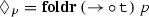 , and
, and  , where
  .
.de Groote (1994) presents a translation of the \(\lambda \mu \)-calculus into the \(\lambda \)-calculus, using a continuation passing style transform. From this perspective, continuation-based proposals (developed extensively in Barker and Shan (2014), although there the focus is on delimited continuations) can be viewed as related to the \(\lambda \mu \)-calculus, and thus to cooper-storage.
Notation has been changed from McBride and Paterson (2008). The operator
 (there called pure) lifts a value into a functor type. This is reflected notationally by having the arrow point up. The operator
  (there written as a binary infix operator
  and known as apply) lowers its argument from a function-container to a function over containers, and so the arrow points down. Viewing \(\bigcirc \) as a necessity operator, the type of
  is familiar as the K axiom, and viewing it as a possibility operator, the type of
  is the axiom T. Lax logic (Fairtlough and Mendler 1997) is the (intuitionistic) modal logic which to the axioms above adds \(\bigcirc \bigcirc \alpha \rightarrow \bigcirc \alpha \) and corresponds via the Curry–Howard correspondance to monads (Moggi 1991; Benton et al. 1998), which are applicative functors enriched with an operation \({\textit{join}} : \bigcirc \bigcirc \alpha \rightarrow \bigcirc \alpha \) satisfying certain conditions.
The parameter arguments will sometimes be suppressed for readability; it is always possible to reconstruct them from the context.
Rather, the equations require only that
 and that
 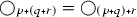 . This is automatic if P is in fact a monoid, but would also be satisfied if, for example, \(\bigcirc \) were the constant function from P into \(\mathcal {T}_A \rightarrow \mathcal {T}_A\).
The applicative functor operations are interdefinable with these, as follows (\(\mathbb {K} = \lambda x,y.x\), \((,) = \lambda x,y.\langle x,y\rangle \), \({\textsf {uncurry}} = \lambda f,x.f (\pi _1 x) (\pi _2 x)\), \({\textsf {app}} = \lambda x,y.xy\), and
 is the empty tuple—the monoidal unit for the product operation).
While the operations and types involving cooper storage are linear, there is no such guarantee about the objects being so manipulated. A natural way to think about this involves treating the types being manipulated as abstract types [as in abstract categorial grammars de Groote (2001a)], the internal details of which are irrelevant to the storage mechanisms.
Except in the uninteresting case where \(w_i = \alpha \) for some i.
A misguided attempt to generalize the current proposal to arbitrary stores is, when attempting to store something of type
 , to put the entire expression of type
  into the store (Kobele 2006). This would yield an alternative storage operator
  . (The given
  would correspond to
  .) While such a generalization is logically possible, it is problematic in the sense that there is no obvious way for the other elements in the store to bind what should intuitively be their arguments, which have been abstracted over in the newly stored expression.
More precisely,
 is a forest of unranked trees. For
  , \(\epsilon \), \(a(\epsilon )\), and \(a(b(\epsilon ),c(\epsilon )),d(\epsilon )\) are elements of P. The term \(a(\epsilon )\) will be written as a, and so these elements of P will be represented rather as \(\epsilon \), a, and a(b, c), d.
The rules in the figure are only annotated with a semantic component, the pronounced components remain the same as in Fig. 1.
As in example 2, the rule for retrieve is non-deterministic.
Where size is measured in terms of the sum of the sizes of the types is the store; this bounds as well the maximal size of stored types.
A short Coq development of this proof is available at https://github.com/gkobele/cooper-storage.
 , and
, and  , where
  .
. (there called
  (there written as a binary infix operator
  and known as
  is familiar as the K axiom, and viewing it as a possibility operator, the type of
  is the axiom T. Lax logic (Fairtlough and Mendler
  and that
  . This is automatic if P is in fact a monoid, but would also be satisfied if, for example,
  is the empty tuple—the monoidal unit for the product operation).
 , to put the entire expression of type
  into the store (Kobele
  . (The given
  would correspond to
  .) While such a generalization is logically possible, it is problematic in the sense that there is no obvious way for the other elements in the store to bind what should intuitively be their arguments, which have been abstracted over in the newly stored expression.
 is a forest of unranked trees. For
  ,
, References
Atkey, R. (2009). Parameterized notions of computation. Journal of Functional Programming, 19(3–4), 335–376.
Babaev, A. A., & Soloviev, S. V. (1982). A coherence theorem for canonical morphisms in cartesian closed categories. Journal of Soviet Mathematics, 20, 2263–2279.
Barendregt, H., Dekkers, W., & Statman, R. (2013). Lambda calculus with types. Cambridge: Cambridge University Press.
Barker, C., & Shan, C. (2014). Continuations and natural language, Oxford studies in theoretical linguistics (Vol. 53). Oxford: Oxford University Press.
Benton, P. N., Bierman, G. M., & de Paiva, V. (1998). Computational types from a logical perspective. Journal of Functional Programming, 8(2), 177–193.
Büring, D. (2004). Crossover situations. Natural Language Semantics, 12(1), 23–62.
Church, A. (1940). A formulation of the simple theory of types. Journal of Symbolic Logic, 5(2), 56–68.
Cooper, R. (1983). Quantification and syntactic theory. Dordrecht: D. Reidel.
de Groote, P. (1994). A CPS-translation of the \(\lambda \mu \)-calculus. In S. Tison (Ed.), Proceedings of the colloquium on trees in algebra and programming—CAAP’94, lecture notes in computer science (Vol. 787, pp. 85–99). Berlin: Springer.
de Groote, P. (2001a). Towards abstract categorial grammars. In Association for computational linguistics, 39th annual meeting and 10th conference of the European chapter, proceedings of the conference (pp. 148–155).
de Groote, P. (2001b). Type raising, continuations, and classical logic. In R. van Rooy, & M. Stokhof (Eds.), Proceedings of the thirteenth amsterdam colloquium (pp. 97–101). Amsterdam: University of Amsterdam.
de Groote, P., Pogodalla, S., & Pollard, C. (2011). About parallel and syntactocentric formalisms: A perspective from the encoding of convergent grammar into abstract categorial grammar. Fundamenta Informaticae, 106(2–4), 211–231.
Fairtlough, M., & Mendler, M. (1997). Propositional lax logic. Information and Computation, 137(1), 1–33.
Hunter, T. (2010). Relating movement and adjunction in syntax and semantics. Ph.D. thesis, University of Maryland.
Johnson, K. (2000). How far will quantifiers go? In R. Martin, D. Michaels, & J. Uriagereka (Eds.), Step by step: essays on minimalist syntax in honor of Howard Lasnik, chap 5 (pp. 187–210). Cambridge, MA: MIT Press.
Kanazawa, M. (2007). Parsing and generation as datalog queries. In Proceedings of the 45th annual meeting of the association of computational linguistics (ACL) (pp. 176–183). Prague: Association for Computational Linguistics.
Kanazawa, M. (2009). The pumping lemma for well-nested multiple context-free languages. In V. Diekert & D. Nowotka (Eds.), Developments in language theory, lecture notes in computer science (Vol. 5583, pp. 312–325). Berlin: Springer.
Kanazawa, M. (2017). Parsing and generation as Datalog query evaluation. The IfCoLog Journal of Logics and their Applications, 4(4), 1103–1211.
Keller, W. R. (1988). Nested cooper storage: The proper treatment of quantification in ordinary noun phrases. In U. Reyle & C. Rohrer (Eds.), Natural language parsing and linguistic theories, number 35 in studies in linguistics and philosophy (pp. 432–447). Dordrecht: D. Reidel.
Kobele, G. M. (2006). Generating copies: An investigation into structural identity in language and grammar. Ph.D. thesis, University of California, Los Angeles.
Kobele, G. M. (2012). Importing montagovian dynamics into minimalism. In D. Béchet & A. Dikovsky (Eds.), Logical aspects of computational linguistics, lecture notes in computer science (Vol. 7351, pp. 103–118). Berlin: Springer.
Kreisel, G., & Krivine, J. L. (1967). Elements of mathematical logic (model theory). Amsterdam: North-Holland.
Larson, R. K. (1985). Quantifying into NP. http://semlab5.sbs.sunysb.edu/~rlarson/qnp.pdf.
May, R., & Bale, A. (2005). Inverse linking. In M. Everaert & H. van Riemsdijk (Eds.), The Blackwell companion to syntax, chap 36 (Vol. 2, pp. 639–667). Oxford: Blackwell.
McBride, C., & Paterson, R. (2008). Applicative programming with effects. Journal of Functional Programming, 18(1), 1–13.
Melliès, P. A. (2017). The parametric continuation monad. Mathematical Structures in Computer Science, 27(5), 651–683.
Michaelis, J. (2001). On formal properties of minimalist grammars. Ph.D. thesis, Universität Potsdam.
Moggi, E. (1991). Notions of computation and monads. Information and Computation, 93(1), 55–92.
Montague, R. (1973). The proper treatment of quantification in ordinary English. In J. Hintikka, J. Moravcsik, & P. Suppes (Eds.), Approaches to natural language (pp. 221–242). Dordrecht: D. Reidel.
Parigot, M. (1992). \(\lambda \mu \)-calculus: An algorithmic interpretation of classical natural deduction. In A. Voronkov (Ed.), Logic programming and automated reasoning, lecture notes in computer science (Vol. 624, pp. 190–201). Berlin: Springer.
Paterson, R. (2012). Constructing applicative functors. In J. Gibbons & P. Nogueira (Eds.), Mathematics of program construction, lecture notes in computer science (Vol. 7342, pp. 300–323). Berlin: Springer.
Pollard, C. (2011). Covert movement in logical grammar. In S. Pogodalla, M. Quatrini, & C. Retoré (Eds.), Logic and grammar: Essays dedicated to Alain Lecomte on the occasion of his 60th birthday, lecture notes in artificial intelligence (Vol. 6700, pp. 17–40). Berlin: Springer.
Seki, H., Matsumura, T., Fujii, M., & Kasami, T. (1991). On multiple context-free grammars. Theoretical Computer Science, 88, 191–229.
Stabler, E. P. (1997). Derivational minimalism. In C. Retoré (Ed.), Logical aspects of computational linguistics, lecture notes in computer science (Vol. 1328, pp. 68–95). Berlin: Springer.
Stabler, E. P., & Keenan, E. L. (2003). Structural similarity within and among languages. Theoretical Computer Science, 293, 345–363.
Vijay-Shanker, K., Weir, D., & Joshi, A. (1987). Characterizing structural descriptions produced by various grammatical formalisms. In Proceedings of the 25th meeting of the association for computational linguistics (pp. 104–111).
Acknowledgements
My thanks to Chris Barker, Dylan Bumford, Simon Charlow, Itamar Francez, Philippe de Groote, and Carl Pollard for their feedback.
Author information
Authors and Affiliations
Corresponding author
Proofs
Proofs
The purpose of this section is to provide a proof of Theorem 3, that graded applicative functors are closed under composition.Footnote 22 It is helpful to first prove a lemma that, for any applicative functor  ,
,  distributes over composition.
Lemma 1
If  is a graded applicative functor, then for any \(p \in P\), \(g : \beta \rightarrow \gamma \) and \(f : \alpha \rightarrow \beta \),
Proof

\(\square \)
Theorem 3 is repeated below.
Theorem 7
Let \(\mathbf {P}\) be a monoid, and let  be graded applicative functors. Then \(\bigcirc \) is a graded applicative functor, where
  , with

The following lemma identifies a useful equality.
Lemma 2

Proof

\(\square \)
Proof
(Proof of Theorem 3) Note first that  , and that
  , as can be seen by inspection of the definitions.
identity

composition

homomorphism

interchange

\(\square \)
Rights and permissions
About this article

Cite this article
Kobele, G.M. The Cooper Storage Idiom. J of Log Lang and Inf 27, 95–131 (2018). https://doi.org/10.1007/s10849-017-9263-1
Published:
Issue Date:
DOI: https://doi.org/10.1007/s10849-017-9263-1