
Abstract
Super-peer networks refer to a class of peer-to-peer networks in which some peers called super-peers are in charge of managing the network. A group of super-peer selection algorithms use the capacity of the peers for the purpose of super-peer selection where the capacity of a peer is defined as a general concept that can be calculated by some properties, such as bandwidth and computational capabilities of that peer. One of the drawbacks of these algorithms is that they do not take into consideration the dynamic nature of peer-to-peer networks in the process of selecting super-peers. In this paper, an adaptive super-peer selection algorithm considering peers capacity based on an asynchronous dynamic cellular learning automaton has been proposed. The proposed cellular learning automaton uses the model of fungal growth as it happens in nature to adjust the attributes of the cells of the cellular learning automaton in order to take into consideration the dynamicity that exists in peer-to-peer networks in the process of super-peers selection. Several computer simulations have been conducted to compare the performance of the proposed super-peer selection algorithm with the performance of existing algorithms with respect to the number of super-peers, and capacity utilization. Simulation results have shown the superiority of the proposed super-peer selection algorithm over the existing algorithms.
1 Introduction
Peer-to-peer networks are large scale computer networks in which each peer simultaneously plays two roles: “client” and “server”. These networks can be extremely dynamic because the peers freely join and leave the network. In these networks, peers can be very different from each other in their properties (such as size of storage, and computational power). Peer-to-peer networks can be classified into two classes [1]: pure peer-to-peer networks and super-peer networks. In pure peer-to-peer networks, the network management algorithms are distributed among all peers. In super-peer networks, some peers are selected to manage the network. In these networks, each super-peer manages a set of peers. Reported algorithms for super-peer selection can be categorized into two categories as described below.
-
Non-adaptive super-peer selection algorithms: In these algorithms, the selection is performed locally at each peer without considering conditions of peers of the network. Because of simplicity, some of peer-to-peer networks such as those reported in [2,3,4,5,6,7] utilize non-adaptive super-peer selection algorithms. In real applications of peer-to-peer network, non-adaptive super-peer selection algorithms suffer from several drawbacks; lack of scalability and lack of robustness to the changes that occur in the network.
-
Adaptive super-peer selection algorithms: In these algorithms such as those reported in [8,9,10,11,12,13,14,15], the super-peer selection algorithms select super-peers based on information about conditions of peers such as number of peers, computational power of peers, or current load on super-peers in a self-organized manner. A group of adaptive super-peer selection algorithms such as those reported in [8, 11, 15, 16] uses the capacity of the peers where the capacity of a peer is computed based on properties such as bandwidth and computational capabilities of that peer.
An approach for designing management algorithms in peer-to-peer networks is based on biologically inspired self-organized models such as models of fungal growth and growing neural gas because they have attractive characteristics such as self-healing, which leads to resilience to changes in the network [11, 14, 17,18,19,20,21,22]. In real applications of peer-to-peer networks, the management algorithms should be resilient to changes in the network because of high rate of changes in the network caused by joining or leaving peers. In order to solve the super-peer selection problem considering peers capacity based on biologically inspired self-organized model, Myconet algorithm was reported in [11]. Myconet algorithm utilizes a self-organized model inspired from a model of growth pattern of fungi to manage the growth and maintenance of the super-peer network.
A problem of Myconet is that its self-organized model has no adaptive mechanism to adjust its rules and parameters with the dynamic conditions of the peer-to-peer networks and also avoid local optima. Therefore, the network dynamicity caused by catastrophic failures and joining (or leaving) peers may conduct the super-peer network to rapidly converge to local optima.
Cellular learning automata(CLAs) are obtained from combination of cellular automata and learning automata [23]. CLAs inherit the distributed computation from the CAs and learning in unknown environments from the LAs. Because of distributed adaptation capability of the CLAs, they have found application in computer networks [24,25,26,27]. These models have been also used in areas such as social networks [28], Petri nets [29], and evolutionary computing [30] to mention a few. Recently, dynamic models of CLAs (DCLAs) have been reported in [24, 31], and [32].
In this paper, an adaptive super-peer selection algorithm considering peers capacity based on an asynchronous dynamic cellular learning automaton will be proposed. The proposed cellular learning automaton uses the model of fungal growth to adjust the attributes of the cells of the cellular learning automaton in order to take into consideration the dynamicity that exists in peer-to-peer networks in the process of super-peers selection. The proposed CLA in which a model of fungal growth is used to adjust the attributes of its cells will be used as a mechanism for selection of the super-peers in peer-to-peer networks. The difference between the super-peer selection algorithm proposed in this paper and Myconet algorithm [11] which also uses a model of fungal growth is that 1.) the fungal growth model is fused with a dynamic CLA used for the purpose of super peer selection and 2.) the fungal growth model fused with CLA is different from the one used in Myconet algorithm. The fusion of fungal growth model with CLA brings together adaptive and distributed computation characteristics in unknown environments from CLA and resilience to changes in the environment from fungal growth model. In contrast to Myconet which uses a simple fungal growth model and it is not able to escape from local optima solutions, this fusion enables the fungal growth model to escape from local optima solutions because of distributed adaptation capability of the CLA. In order to study the performance of this model, two metrics: entropy and potential energy will be introduced. Computer experimentations have been conducted to study the performance of the proposed super-peer selection algorithm. The results of experiments show that the proposed CLA based super selection algorithm outperforms the existing algorithms with respect to the number of super-peers, and capacity utilization. The remainder of the paper is organized as follows. The problem statement is given in Section 2. In Section 3, related works are briefly described. Section 4 is dedicated to some preliminaries used in this paper. In Section 5, an adaptive algorithm for super-peer selection has been proposed. The results of simulations are reported in Sections 6 and 7 is the conclusion.
2 Problem statement
Consider n peers which are connected to each other through a peer-to-peer network. The topology of the peer-to-peer network can be represented by each graph such as G = (V, E) in which V = {p e e r 1,p e e r 2,...,p e e r n } is a set of peers and E ⊆ V × V is a set of links connecting the peers in the network. In super-peer networks, some peers must be selected as super-peers. The peers which are not selected as super-peers are called as ordinary-peers. The topology of the super-peers network can be represented by a graph G s = (V s,E s) in which V s ⊆ V is a set of super-peers and E s ⊆ V × V is a set of links connecting the super-peers in the super-peer network. In a super-peer network, each super-peer in V s is mapped to several ordinary-peers in V according to an one-to-many function H : V s → V. Figure 1 shows an example of a peer-to-peer network which uses three super-peers. In this example, peer m , peer j , and peer q are three super-peers.

An example of super-peer network with three super-peers
In the super-peer networks, the network management responsibilities are handled by the super-peers. In these networks, the network communications are done among super-peers. A super-peer network with a large number of super-peers imposes a large overhead to the network with respect to control messages generated by the management algorithms of the super-peers. Therefore the existing algorithms such as those reported [8, 11, 15, 16] try to adaptively select a small set of super-peers considering some metrics such as peers capacity in distributed fashion.
In [33], different types of the super-peer selection problems has been compared with classic problems such as dominating set, p-centers, and leader election. In super-peer networks such as those reported in [8, 11, 15, 16], variable c i (called capacity) to save the number of peers that can be handled by peer i if peer i is selected as super-peer in the network is defined. The value of variable c i is determined when peer i joins the network and it remains constant throughout the operation of the network. Since, the goal of super-peer selection considering peers capacity sounds a lot like capacitated minimum vertex cover algorithms, some required definitions about capacitated minimum vertex cover are given as below.
Definition 1
A vertex cover V c of graph is a subset of V such that (u, v) ∈ E → u ∈ V c or v ∈ V c. Such a set is said to vertex cover of G [34].
Definition 2
A minimum vertex cover is a vertex cover which it has the smallest possible size. The problem of finding a minimum vertex cover is an NP-hard problem [34].
Definition 3
A capacitated minimum vertex cover is a minimum vertex cover in which there is a limit to the number of edges that a vertex can cover [35].
According to the mathematical formulation of capacitated vertex cover problem reported in [35], In order to solve the super-peer selection problem considering peers capacity the following problem should be solved.
In (1), the values of x v correspond to cost of selecting a peer peer v as a super-peer for a super-peer network. In (2), y e v = 1 if and only if the link corresponding to edge e ∈ E is connected to peer peer v . Constraint (2) says that every peer must be connected to one super-peer. For any peer peer v , let E(v) denote the set of links peer v . In (3), c v denotes the capacity of peer peer v (we assume that c v is an integer). Constraint (3) guarantees that the number of links of a peer peer v cannot be more than its capacity. Constraint (4) guarantees that ordinary-peers cannot connect to another ordinary-peer.
Since no global knowledge about the network exists and the conditions of the network are highly dynamic, minimizing (1) subject to (3)–(6) by the super-peer selection algorithm leading to a challenging problem. Therefore the existing algorithms such as those reported [8, 11, 15, 16] try to adaptively select a small set of super-peers considering capacity of the peers.
3 Related work
In the review of the relevant literature, we focus on adaptive super-peer selection algorithms. In adaptive super-peer selection algorithms, the selection algorithms use local information (such as lifetime and capacity of peers) or global information (such as end-to-end delay or lifetime) about peers.
In [10], Dynamic Layer Management (DLM) which is a layered management mechanism is reported for file sharing applications. DLM tries to select super-peers using information about age and capacity of peers adaptively. In DLM, capacity is defined as the ability of a peer to process and relay queries and age is defined as the length of time during which the peer participates in the network since it joined the network. In [36], DLM is improved by particle swarm optimization algorithm. In [37], a weighted metric based on content similarity is used to select super-peers for file sharing applications. In [38], an algorithm for super-peer selection is proposed which uses upload capacity of the peers in its super-peer selection algorithm. This algorithm is specific for video streaming system. In [39,40,41,42], semantic similarity of peers is used to create super-peer network. The peers that share the same interest are connected to the same super-peers. These algorithms are designed to improve the search efficiency rather than the efficiency of creating super-peer network. In [43], the online time of peers is used to construct a super-peer network. This algorithm is appropriate for live streaming systems. A main problem of [10, 36,37,38,39,40,41,42,43], is that these algorithms are specific to file-sharing and video streaming applications and we cannot easily extend them to other type of peer-to-peer applications.
In [13, 44,45,46], gradient topologies are reported. In gradient topologies, the super-peer selection algorithm utilizes a function called utility function, which can be defined based on every computable metric in the peer. A problem of gradient topologies is that they do not consider the proximity among peers in its super-peer selection algorithm. In [14], a super-peer selection algorithm based on growing neural gas model is presented. This algorithm considers the proximity among peers in its super-peer selection algorithm in order to decrease the communication delay between peers. This algorithm does not consider the capacities of the peers. In SG-1 [8], the super-peer selection algorithm uses a general concept called capacity in its selection algorithm. Capacity is defined as a general metric that can be calculated by some properties such as bandwidth and size of storage and computational power. The goal of SG-1 is to adaptively select super-peers considering peer capacities. SG-1 does not consider several important factors such as proximity of peers which affects communication delay among peers. To solve this problem, SG-2 is reported in [9]. SG-2 is an extension to SG-1 which uses information about proximity of peers in selecting super-peers. SG-2 tries to localize the super-peer selection algorithm of SG-1, but many problems are still remaining. A problem of SG-1 is that its convergence speed is low. This is because each peer in SG-1 uses limited information about the network. To solve this problem SPS was proposed in [16]. SPS uses the structure of SG-1 and utilizes local search operations to provide enough information for each peer which leads to improving the speed of convergence of the algorithm. Since providing information for the peers of the network by the search operations results in generating many messages, the overhead of the SPS is higher than SG-1. One of the problems of both SG-1 and SG-2 is that they are not able to adapt themselves to dynamic conditions of peer-to-peer networks. In [15], SG-LA which is an adaptive version of SG-1 is reported. SG-LA improves the super-peer selection algorithm of SG-1 with learning capability of learning automata.
All SG-1, SG-LA, and SPS algorithms suffer from lack of a self-organizing mechanism which is resilient to the changes that occur in the network. This problem is solved by Myconet algorithm which is a biologically inspired super-peer selection algorithm [11]. In this algorithm, a model of growth pattern of fungi is used as a self-organizing model in the super-peer selection algorithm in order to improve the self-healing capability of the super-peer network. A problem of Myconet is that its self-organizing model has no adaptive mechanism to escape from local optima solutions and also adapt with dynamic conditions in peer-to-peer networks. This problem affects the efficiency of the super-peer selection algorithm of Myconet. In [12], a super-peer selection algorithm based on peer’s capacity and online time was given which is able to select appropriate stable peers. Note that the online time was not used in SG-1, SG-2, Myconet and SG-LA.
Table 1 summarizes the related works with respect to requirements on management algorithms in peer-to-peer network such as scalability, self-organization, and robustness. In addition, other specifications explicitly mentioned in the literature such as application dependency and extra information usages are also reported in this table.
In this paper, an adaptive algorithm utilizing a new model of CLAs for super-peer selection will be proposed. The algorithm proposed in this paper similar to SG-1, SG-2, SG-LA, SPS and Myconet algorithms use capacities of the peers and similar to Myconet algorithm is inspired from growth pattern of fungi. The difference between the super selection algorithm proposed in this paper and Myconet algorithm [11] which also uses a model of fungal growth is that 1. The fungal growth model is fused with a dynamic CLA used for the purpose of super peer selection and 2. The fungal growth model fused with CLA is different from the one used in Myconet algorithm.
4 Preliminaries
In this section, in order to provide basic information for the remainder of the paper, we present a brief overview of cellular learning automata and growth pattern of fungi reported.
4.1 Cellular learning automata
In this section, cellular automata, learning automata and cellular learning automata are reviewed.
Cellular Automata (CAs)
CAs are computational models which are composed of independent and identical cells. In these models, the cells are arranged into a lattice. In aCA, each cell selects a state from a finite set of states. A cell uses the previous states of a set of cells, including the cell itself, and its neighbors and then updates its state using a rule called local rule. CAs evolves in discrete time steps [47, 48]. CAs can be also classified as static CAs or dynamic CAs. In static CAs, the structure of the cells remains fixed during the evolution of the CA whereas In dynamic CAs, the structure of the cells or the local rule changes during the evolution of the CA [49, 50] and [51]. CAs can be classified as synchronous CAs or asynchronous CAs. In synchronous CAs the states of all cells in different cells are updated synchronously whereas in asynchronous CAs the states in different cells are updated asynchronously. Different types of cell activation methods for asynchronous CAs have been described in the literature [52,53,54] some of which are described below:
-
The random independent: in this method, a cell is randomly selected at each time step and then activated.
-
The random order: in this method, a random order of cells is determined at each time step. This order is used to activate the cells during that time step. A new random order of cells will be used for cells activation for the next time step.
-
Cyclic: in this method, at each time step, a node is chosen according to a fixed activation order which is part of the definition of the CA.
-
Clocked: in this method, each cell has an independent timer. The timer is initialized to a random period. When the period has expired, the cell is activated and then the timer is reset.
CAs depending on their structure can be also classified as regular CAs or irregular CAs. In Irregular CAs, the structure regularity assumption has been relaxed [55]. The irregular CAs and CAs with structural dynamism, can be generalized and obtain models which are known as automata networks in the literature. An automata network is a mathematical system consisting of a network of nodes that evolves over time according to a predetermined rules [56, 57]. Since the definition of automata networks has fewer restrictions on the network of nodes and also evolution of the structure of the automata than the CAs, the automata networks are considered as a general model for CAs.
Learning Automata (LAs)
LAs are models for adaptive decision making in random environments. The relationship between an LA and its environment is shown in Fig. 2. A set of actions has been defined for this model. Each action has a probability which is unknown for the LA for getting rewarded by the environment. This model tries to find an appropriate action through repeated interaction with the environment. The appropriate action is an action with the highest probability of getting reward by the environment. Each time the LA interacts with its environment, it randomly selects an action based on a probability vector. According to the response of the environment (reward or penalty) to the selected action, the LA updates its action probability vector and then the procedure is repeated. The updating algorithm for the action probability vector is called the reinforcement scheme or the learning algorithm. If the learning algorithm is chosen properly, then the iterative process of interacting with the environment can be set up to result in selection of the optimal action. The interaction between LA and the environment is shown in.

Learning Automaton (LA)
Learning automata can be classified into two main families, fixed and variable structure learning automata [58, 59]. Variable structure learning automata which are used in this paper is represented by sextuple < β, ϕ, α, P, G, T>, where β is a set of inputs actions (called response or reinforcement signal), \(\underline {\upphi }\) is a set of internal states, \(\underline {\upalpha }\) is a set of outputs, P denotes the state probability vector governing the choice of the state at each stage k, G is the output mapping, and T is learning algorithm. The learning algorithm is a recurrence relation and is used to modify the state probability vector.
It is evident that the crucial factor affecting the performance of the variable structure learning automata is the learning algorithm for updating the action probabilities. Let αi ∈{α1,α2,…,αr} be the action chosen at time k as a sample realization from distribution p(k). The linear reward-penalty algorithm (L RP) is one of the earliest schemes. In an L RP scheme the recurrence equation for updating probability vector p is defined by (7) for favorable responses (β = 1), and (8) for unfavorable response (β = 0).
The parameters a and b represent reward and penalty parameters, respectively. The parameter a(b) determines the amount of increase (decreases) of the action probabilities. Learning automata have found applications in many areas such as sensor networks [24, 30], stochastic graphs [60], peer-to-peer networks [15, 61,62,63,64], channel assignment [65], mobile cloud computing [66] to mention a few.
Cellular Learning Automata (CLAs)
[23] A CLA is a CA in which a LA is assigned to each cell (Fig. 3). The LA residing in a particular cell determines its state (action) according to its action probability vector. This model is superior to CA because of its ability to learn and is also superior to single LA because it consists of a collection of LA s interacting with each other. Like CA, there is a local rule that the CLA operates under. The local rule of the CLA and the actions selected by the neighboring LA s of any particular LA determine the reinforcement signal to that LA. The neighboring LA s (cells) of any particular LA (cell) constitute the local environment of that LA (cell).

A cellular learning automaton [23]
Several models of CLAs are reported in the literature. The reported models can be classified into two main classes as described below.
-
Static CLAs (SCLAs) : In a SCLA, the structure of the cells remains fixed during the evolution of the SCLA [28, 67,68,69,70,71]. SCLAs can be either closed or open. In closed SCLAs, the states of neighboring cells of each cell called local environment affects on the action select ion process of the LA of that cell whereas in open SCLAs, the local environment of each cell, a global environment, and an exclusive environment effects on the action selection process of the LA of that cell. In an open SCLA, each cell has its own exclusive environment and one global environment defined for the whole SCLA. SCLAs can be further classified as either synchronous or asynchronous. In a synchronous SCLA, all cells perform their local rules at the same time [67]. This model assumes that there is an external clock which triggers synchronous events for the cells. In asynchronous SCLA, at a given time only some cells are activated and the state of the rest of cells remains unchanged [68]. In [69], a model of SCLA with multiple LAs in each cell was reported. In this model, the set of LAs of a cell remains fixed during the evolution of the SCLA. SCLA depending on its structure can be also classified as regular [23] or irregular [70]. In Irregular SCLA, the structure regularity assumption is removed.
-
Dynamic CLAs(DCLAs): In a DCLA, one of its aspects such as structure, local rule, attributes or neighborhood radius may change over time. DCLAs can be classified as either closed DCLAs [24, 31, 32, 72] or open DCLAs. DCLAs can also be also classified as synchronous DCLAs or asynchronous DCLAs. In synchronous DCLAs, all LAs in different cells are activated synchronously whereas in asynchronous DCLA s the LAs in different cells are activated asynchronously. Asynchronous DCLAs can be either time-driven or step- driven [31]. In time-driven asynchronous DCLAs, each cell is assumed to have an internal clock which wakes up the LA associated to that cell while in step-driven asynchronous DCLAs, a cell is selected in fixed or random sequence. Note that, the problem of the definition of asynchronous DCLAs is application dependent. All the reported DCLAs are closed and asynchronous [24, 31, 32, 72]. DCLAs can be also classified as interest based DCLAs [24, 31] or attribute based DCLAs [32]. In interest based DCLAs, a set of interests is defined for describing the dynamicity of the CLA and in attribute based DCLAs, a set of attributes is defined for describing the dynamicity of the CLA. A main drawback of both interest based DCLAs and attribute based DCLAs is that there is no formal definitions for the rules which determine the changes in the attributes or interests of the cells. Therefore the existing models of DCLAs are unable to support dynamicity in a wide range of application with changing attributes or interests. In this paper, this problem will be solved by suggesting a dynamic model of the CLA with changing attributes.
4.2 A brief description about the growth pattern of fungi
In nature, fungi reproduce by extending filamentous strands through a growth medium such as the soil (Fig. 4). The filamentous strands are called Hyphae. A Hypha (plural Hyphae) is a long, branching filamentous structure of a fungus. Fungi follow an interesting pattern of growth. They do not follow a fixed evolutionary pathway. The growth pattern of a fungus is very flexible because all cells of a Hyphae may initiate a colony. The mechanism used for formation of colonies of fungi is determined by the water and nutrients of the soil of the environment. Hypha cells are able to sense reproductive cells from distance, and grow towards them. In order to find new resources, Hypha cells are also able to penetrate to the permeable surfaces during reproduction. Different classifications considering the cell, structure, and growth pattern of fungi are reported in the literature [73, 74].

An example for growth pattern of fungi [74]
5 Proposed algorithm
In this section, we first present a state machine inspired from growth pattern of fungi, then suggest a new model of CLAs, and finally outline the proposed super-peer selection algorithm.
5.1 A state machine inspired from growth pattern of fungi
The state machine is described as follows (Fig. 5). Each cell takes one of three types: Unattached-Cell, Attached-Cell, and Colony-Manager. The initial type of all cells is set to Unattached-Cell. Each Unattached-Cell cell tries to find a Colony-Manager cell from its neighbors. In Unattached-Cell cell i , after finding a Colony-Manager cell j , cell i changes its type to Attached-Cell (Transition 1). If cell i couldn’t find any Colony-Manager cell then it changes its type to Colony-Manager (Transition 2). If a Colony-Manager cell i is connected to a Colony-Manager cell j which the capacity of cell j is greater than the capaci ty of cell i , then cell i changes its type to Attached-Cell (Transition 3). If an Attached-Cell cell i is connected to Colony-Manager cell j and the capacity of cell i is greater than the capacity of cell j , and all Attached-Cell cells that are connected to the cell j then cell i changes its type to Colony-Manager (Transition 4).

The state machine inspired from growth pattern of fungi
Each Colony-Manager cell takes one of two states: Colony-Extender, and Colony-Immobilizer. If the state of a cell is equal to Colony-Extender, the cell can be connected to Colony-Extender, and Colony-Immobilizer cells. If the state of a cell is equal to Colony-Immobilizer, the cell can be connected to Colony-Immobilizer cells. A Colony-Immobilizer cell is able to absorb the Attached-Cell cells of other Colony-Immobilizer and Colony Extender cells. A Colony-Extender cell is able to absorb the Attached-Cell cells of other Colony-Extender cells.
Since, this state machine is merged into the ADCLA, the mechanisms used for selecting the state of a cell, and changing the connections among the cell will be described in more details later in the proposed algorithm.
5.2 Asynchronous dynamic cellular learning automaton with changing attribute (ADCLA-CH)
An ADCLA-CH is a network of cells whose structure and the attributes of the cells change with time. This model can be formally defined by a 10-tuple A D C L A − C H = (G, A, N,Φ,Ψ,F 1,F 2,F 3,F 4,F 5), where:
-
G = (V, E) is an undirected graph which determines the structure of ADCLA-CH where
V = {c e l l 1,c e l l 2,…,c e l l n } is the set of vertices and E is the set of edges.
-
A = {L A 1,L A 2,…,L A n } is a set of LAs each of which is assigned to one cell of ADCLA-CH. The set of actions of automaton for a cell is the same as the set of states for that cell.
-
N = {N1,N2,…,N n } where N i = {c e l l j ∈V | d i s t(c e l l i ,c e l l j ) < 𝜃 i} where 𝜃 i is the neighborhood radius of c e l l i and d i s t(c e l l i ,c e l l j ) is the length of the shortest path between c e l l i and c e l l j in G. \({N_{i}^{1}}\) determines the immediate neighbors of cell i which constitute its local environment.
-
Ψ = {Ψ1,Ψ2,…,Ψ n } where Ψi = {(j, X j) | c e l l j ∈ N i } denotes the attribute of cell j where X j ⊆{x 1,x 2,…,x s }. {x 1,x 2,…,x s } is the set of allowable attributes. \({{\Psi }_{i}^{1}} \) determines the attribute of cell i when 𝜃 i = 1.
-
Φ = {Φ1,Φ2,…,Φ n } where Φi = {(j, α l )| c e l l j ∈ N i and action α l has been chosen by L A j } denotes the state of cell i . \({\Phi }_{i}^{1}\) determines the state of cell i when 𝜃 i = 1.
-
\(F_{1}:\left ({\underline {\Psi }} \right )\to (\underline {\zeta })\) is the restructuring function. In each cell, the restructuring function computes the restructuring signal based on the attributes of the cell and its neighboring cells. For example, in cell i , the restructuring function takes <Ψ i > and then returns a value from the closed interval [0,1] for \(\zeta _{i}^{1}\) which is the restructuring signal of cell i . we define \(\zeta _{i}=\left \{ \left (j,\zeta _{j}^{1} \right )\vert \ {cell}_{j}\in N_{i}\right \}\) to be the set of restructuring signals of neighbors of cell i . In a cell, depending on the application, the value of the restructuring signal determines whether the neighbors of that cell should be changed or not. If the \(\zeta _{i}^{1}\) is equal to zero (one) this means that the neighbors of cell i are appropriate (not appropriate).
-
\(F_{2}:\left (\underline {N}, \underline {\Psi },\underline {\zeta } \right )\to (\underline {N}^{1})\) is the structure updating rule. In each cell, the structure updating rule finds the immediate neighbors of the cell based on the restructuring signal computed by the cell, the attributes of the neighbors of the cell, and the neighbors of the cell. For example, in cell i , < N i ,Ψ i ,ζ i ,> and returns \(<N_{i}^{1}>\).
-
\(F_{3}:\left (\underline {\zeta }\right )\to (\underline {\nu })\) is the automaton trigger function. Upon activation of a cell, automaton trigger function is called to determine whether the learning automata residing in that cell are to be triggered or not. If the automaton trigger function returns true, then the learning automata of the cell will be triggered. The automaton trigger function in cell i takes < ζ i > and returns a value from {true, false} for ν i where ν i is called automaton trigger signal. In a cell, since the value of the restructuring signal affects the changes in the composition of the neighboring cells of that cell, the value of the restructuring signal is used to determine the value of the automaton trigger signal. In cell i , if the ν i is equal to true (false), then the learning automata of cell i are triggered (not triggered).
-
\(F_{4}:\left (\underline {\Phi },\underline {\Psi }\right )\to \left (\underline {\beta }\right )\) is the local rule of ADCLA-CH. In each cell, the local rule computes the reinforcement signal for the learning automata of that cell based on the states and the attributes of that cell and its neighboring cells. For example, in cell i , local rule takes <Φ i ,Ψ i > and then computes the reinforcement signal < β i > for the learning automata of cell i .
-
\(\mathrm {F}_{5}:(\underline {\Psi })\to (\underline {\Psi }) \) is the attribute transition rule. In each cell, the attribute transition rule computes the attribute of the cell. For example, in cell i , attribute transition rule takes <Ψ i > and returns set Ψ i as the set of attributes of cell i .
The application determines which cell must be activated. Upon the activation of a cell, the cell performs a process which has three phases: preparation, structure updating and state updating. These three phases are described below.
- 1) Preparation phase: :
-
In this phase, a cell performs the following steps.
-
Step.1
: The cell computes its attribute using the attribute transition rule (F 5).
-
Step.2
: The cell and its neighboring cells compute their restructuring signals using the restructuring function (F 1).
-
Step.1
- 2) Structure updating phase: :
-
In this phase, a cell performs the following steps.
-
Step.1
: The neighborhood structure of the cell is updated using the structure updating rule (F 2) if the value of the restructuring signal of that cell is 1.
-
Step.2
: The automata trigger function (F 3) depending on the restructuring signal determines whether the set of LAs of the cell must be triggered or not.
-
Step.3
: If the LAs are triggered then the cell goes to the state updating phase
-
Step.4
: If the set of LAs of the cell are not triggered then the activation process terminates.
-
Step.1
- 3) State updating phase: :
-
In this phase, a cell performs the following steps.
-
Step.1
: Each LA of the cell selects one of its actions. The set of actions selected by the set of LAs in the cell determines the new state for that cell.
-
Step.2
: The local rule (F 4) is applied and a reinforcement signal is generated according to which the action probability vectors of the LAs of the cell are updated.
-
Step.1
The internal structure of cell i and its interaction with local environments is shown in Fig. 6. In this model, each cell has a LA and four components: attribute updater, restructuring signal generator, structure updater, and automata trigger function as explained below.
-
1.
Attribute updater: this unit computes the attribute using the attribute transition rule.
-
2.
Restructuring signal generator: this unit computes the restructuring signal using the restructuring function.
-
3.
Structure updater: this unit updates the set of neighboring cells of the cell according to the restructuring signal and structure updating rule.
-
4.
Automata trigger function: this unit determines whether the set of LAs of the cell to be triggered or not according to the value of the restructuring signal.

Internal structure of cell i and its interaction with the local environment
5.3 Proposed algorithm: X-NET
Initially, an ADCLA-CH isomorphic to the peer-to-peer network is created which involves defining the initial structure, local rule, structure updating rule, automata trigger function, restructuring function, and local environments (Fig. 7). each peer peer i corresponds to the cell cell i in ADCLA-CH. Each peer may play one of three roles: unattached, ordinary or super. Each peer uses its corresponding cell to set its role and execute appropriate management operation. Each cell may have one of two states: Colony-Extender, and Colony- Immobilizer. Each cell is equipped with a LA which has two actions: Colony-Extender, andColony- Immobilizer to determine the state of the cell. The attribute of cell i consists of two parts: capacity c i and type t i . For a cell, capacity is defined as maximum number of cells which can connect to the cell simultaneously. A cell may take one of three types: Unattached-Cell, Attached-Cell, and Colony-Manager. In each peer, the role of the peer is determined by the type of its corresponding cell (will be described in more details later). The remaining parts of the ADCLA-CH are described later in the rest of this section.

Asynchronous Dynamic Cellular Learning Automata and Peer-to-peer network
Once the ADCLA-CH is created, the proposed algorithm utilizes it to manage the roles of the peers. The process executed by each peer peer i when joining to the network consists of three phases: initialization Phase, construction phase, and maintenance phase. These phases are briefly described as below.
-
Initialization phase: During this phase performed by a peer, the peer establishes its connections to other peers of the network, and initializes its corresponding cell. Then the cell goes to construction phase. During the initialization of the cell, the following settings are used.
-
◦ The initial state of the cell is set to Colony-Extender.
-
◦ The initial type of the cell is set to Unattached-Cell.
-
◦ The neighborhood radius of the cell is set to 2.
-
◦ The value of capacity is determined.
-
-
Construction phase: During this phase performed by a peer, the peer determines its role using its corresponding cell In this phase, the peer activates its corresponding cell. After executing the activation procedure of cell i , peer i sets its role using the type of cell i and goes to maintenance phase. peer i sets its role to super if the type of cell i is equal to Colony-Manager. peer i sets its role to ordinary if the type of cell i is Attached-Cell. peer i sets its role to unattached if the type of cell i is Unattached-Cell.
-
Maintenance phase: In this phase, an ever going process is executed to handle events occurs for the peer or the neighbors.
Now, we complete the description of the algorithm by describing the 1) Attribute updater, 2) Restructuring signal generator, 3) Automata trigger function, 4) Local rule and 5) Structure updater for the ADCLA-CH used by activation procedure in the proposed algorithm.
- 1) Attribute updater: :
-
The input and output of this unit are shown in Fig. 8. This unit applies the attribute transition rule which is described as below.
Fig. 8 
Input and output of the attribute transition rule of cell i
-
1.
Attribute transition rule: In order to change the attribute of the cells, the Attribute transition rule will use the state machine that has been suggested before for growth pattern of fungi. It should be noted that, this state machine is used to change the type of the cells.
-
1.
- 2) Restructuring signal generator: :
-
The input and output of this unit are shown in Fig. 9. Based on the restructuring function, this unit takes information about neighbors of a cell as input and returns a restructuring signal. The restructuring function is described as below.
Fig. 9 
Input and output of the restructuring signal generator of cell i
-
Restructuring function: In a cell, the restructuring signal is set to 1 if the type of that cell is equal to Colony-Manager and 0 otherwise.
-
- 3) Automata Trigger Function: :
-
The input and output of this unit are shown Fig. 10. Based on the automata trigger function, this unit takes the restructuring signal of a cell as input and then returns true or false which determines the learning automata of the cell are activated or not. The automata function is described as below.
Fig. 10 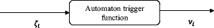
Input and output of the automaton trigger function of cell i
-
Automaton trigger function: In a cell, the automaton trigger function returns true if the restructuring signal of that cell is equal to 1 and false otherwise.
-
- 4) Local environment: :
-
The input and output of this unit are shown in Fig. 11. In this environment, the reinforcement signal β i is computed by applying the local rule. The local rule is described as below.
Fig. 11 
Input and output of the local environment of cell i
-
Local rule: The local rule of cell i returns 1 in three cases described as follows. In the first case, the capacity of the cell i is lower than the capacity of majority of neighboring cells, and the state of cell i is equal to Colony-Extender. In the second case, the capacity of the cell i is higher than the capacity of majority of neighboring cells, and the state of cell i and the majority of states of immediate neighboring cells are equal to Colony-Immobilizer. In the third case, the unused capacity of the cell i is equal to zero, and the state of cell i is equal to Colony-Extender. In other cases, the local rule returns 0.
-
- 5) Structure updater: :
-
The input and output of this unit are shown in Fig. 12. This unit applies the structure updating rule to find the immediate neighbors which determine the local environment. This unit is described as below.
Fig. 12 
Input and output of the structure updater of cell i
-
Structure updating rule: Structure updating rule is implemented using an operator called Absorb operator. Figure 13 shows an example of usage of Absorb operator. In this figure, if the restructuring signal of cell i is equal to 1, and cell i has unused capacity then the structure updating rule selects cell j using a function called candidate-selector() and then randomly chose some of the neighbors of cell j and uses the Absorb operator to transfer the chosen neighbors to cell i for filling the unused capacity of cell i . Function candidate-selector() is described as follows. This function takes information about the neighbors of a cell and then returns one of the neighbors of that cell as output. If the state of a cell is Colony-Immobilizer, then function candidate-selector() randomly selects one of neighboring cell which its state is equal to Colony-Immobilizer, or Colony-Extender, and then returns it. If the type of a cell is Colony-Extender then function candidate-selector() randomly selects one of neighboring cell which its type is equal to Colony-Extender, and then returns it. If function candidate-selector() couldn’t select any cell, the neighbors of cell i remains unchanged.
Fig. 13 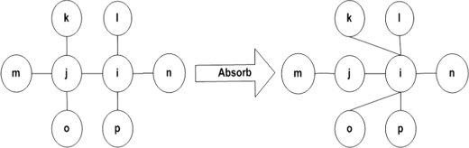
An example for Absorb operation
-


Now, we give the detailed descriptions of the proposed algorithm. The pseudo code of the process executed by a peer i when joining to the network is given in Fig. 14. This process consists of three phases: initialization Phase, construction phase, and maintenance phase. The detailed descriptions of these phases are given in the rest of this section.

Pseudo code of the proposed algorithm
During initialization phase, peer i establishes its connections to other peers of the network, and initializes its corresponding cell cell i . In the initialization phase, peer i finds some peers using Newscast protocol [75] to connect the network. Note that the Newscast protocol is also used in SG-LA, SG-1, and Myconet for establishing initial connections. After establishing the initial connections, peer i initializes its corresponding cell cell i . During initializing cell i , the capacity of cell i is computed and the type of cell i is set to Unattached-Cell. Then peer i goes to construction phase.
During construction phase, peer i determines its role. In the construction phase, peer i executes the activation procedure of its corresponding cell that is cell i . Figure 15 shows the pseudo code of the procedure which each cell of CLA executes after activation. After executing the activation procedure of cell i , peer i sets its role using the type of cell i and goes to maintenance phase. peer i sets its role to super-peer if the type of cell i is equal to Colony-Manager. peer i sets its role to ordinary-peer if the type of cell i is Attached-Cell. peer i sets its role to unattached-peer if the type of cell i is Unattached-Cell.

Pseudo code of the procedure which each cell executes after activation
During the maintenance phase, which is an ever going process, peer i continually waits for one of the events leaving a peer, joining a peer, request for execution of Absorb operation, and request for exchanging information.
If peer i has detected that it has no neighboring peers, it goes to initialization phase. If peer i has detected that join, leave , Absorb operation, or cellular operation has occurred in its neighborhood, it performs appropriate management operation. The management operations are described as below:
-
If peer i has received a request for joining peer from peer j , peer i connects to peer j .
-
If peer i has detected that one of its neighboring peers has left, peer i removes information about that neighbors form the list of its neighbors.
-
If peer i has been activated by a peer j to execute Absorb operation then peer i executes Absorb operation with peer j .
-
If peer i has been activated by a peer j to execute a cellular operation (such as computing restructuring signal, gathering attributes and etc) then peer i executes appropriate operation with peer j .
After executing the management operation, peer i refines the list of its neighbors considering the effects of the management operations and then goes to the construction phase. If peer i has been activated to exchange information with its neighbors, then peer i exchanges information with its neighbors and then restarts the maintenance phase.
6 Experimental results
All simulations have been implemented using OverSim [76]. OverSim is an overlay network simulation framework for peer-to-peer networks which is based on OMNeT + +. The performance of the proposed algorithm which we call itX-NET is compared with four different algorithms Myconet [11], SG-1 [8], SPS [16], and SG-LA [15] among which SG-1 is a well-known super-peer selection algorithm. The reason for selecting these algorithms is that the concept of peer capacity used in these algorithms is similar to the concept of peer capacity used in X-NET.
In order to evaluate the performance of the X-NET, we used two groups of metrics. In the first group, four metrics: Number of Super-Peer (NSP), Peer Transfer Overhead (PTO), Control Message Overhead (CMO), and Capacity Utilization (CU) are used to compare the performance of the X-NET with other super-peer selection algorithms. The definitions of these metrics are given below.
-
NSP is the sum of number of super-peers of the network (z in (1)). The super-peer selection algorithms try to decrease NSP. Higher value of NSP leading to a large set of super-peers which is not appropriate. This metric is used in [8, 11, 15, 16].
-
PTO is the number of peers which are transferred between super-peers. This metric implicitly shows the changes which were made by the operators (such as Absorb operator) of the management algorithms. PTO can be used to study the changes occur in the conf iguration of the super-peer network. Higher value of PTO indicates higher changes in the configuration of the network which is bad. This metric is used in [15, 16].
-
CMO is the number of extra control messages generated by the management algorithm. This metric is used in [15, 16]. Higher value of CMO indicates higher traffic in the network.
-
CU is the ratio of current number of attached clients to total capacity provided by super-peer as given in (9). In (9), let S denote the number of selected super-peers. This metric is used in [11, 15]. If the value of CU becomes one, then the capacity of all super-peers is used. High value for CU is preferred.
In the second group of metrics we have two metrics Entropy and Potential Energy. Theses metrics which are defined below are used to study the performance of ADCLA-CH of the X-NET.
-
Entropy of ADCLA-CH is measured using (10). In the (10), n is the number of LAs of the ADCLA-CH. r k is the number of actions of the LA k . p k l (t) is the probability of selecting action α l of the LA k at iteration t of the ADCLA-CH. Entropy of the ADCLA-CH can be used to study the changes that occur in the states of the cells of ADCLA-CH. The value of zero for H(t) means that the LAs of the cells no longer change their action. Higher values of H(t) mean higher rates of changes in the actions selected by LAs residing in the cells of the ADCLA-CH [24, 31].
-
Potential Energy of ADCLA-CH is measured using (11). \(\zeta _{i}^{1}\ \text {(t)}\) is the restructuring signal of cell i at iteration t. The value of A(t) is used to study the changes in the structure of ADCLA-CH. Potential energy can be used to study the changes in the structure of ADCLA-CH as it interacts with the environment. If the value of A(t) becomes zero then no further change needs to be made to the structure. Higher value of A(t) indicates higher disorder in the structure of ADCLA-CH.
Results reported are averages over 50 different runs. For both X-NET and SG-LA, each peer is equipped with a variable structure learning automaton of type L R P . The reward parameter a and penalty parameter b for L R P are set to 0.25 and 0.25, respectively. To generate the capacities of peers Pareto distribution and Uniform distribution are used. For Pareto distribution the maximum capacity is set to 100 and the parameter \({\mathcal {D}}\) is set to 2, and for Uniform distribution the maximum capacity is set to 100.
Experiment 1 is conducted to study the performance of X-NET with respect to NSP, PTO, CMO, CU, Entropy and Potential Energy. In experiment 2 to experiment 5, X-NET is compared with SG-1, SG-LA, Myconet, and SPS algorithms with respect to NSP, CMO, PTO, and CU. In order to study the performance of X-NET in long run, experiment 1 is perf ormed for 1000 rounds. Other experiments are performed for 100 rounds
- Experiment 1: :
-
This experiment is conducted to study the performance of the proposed algorithm with respect to NSP, PTO, CMO, CU, Entropy and Potential Energy. In this experiment, the network size is 10000 and the power-law distribution is used to generate the capacities of peers. The results of this experiment are given in Figs. 16–21. According to the results of this experiment, we may conclude the following.
-
Figure 16 plots the Entropy versus round during the execution of the algorithm. This figure shows that the value of Entropy is high at early rounds and gradually decreases. This means that the changes in the role taken by a peer frequently occur during the early rounds and becomes less frequent in the later rounds.
-
Figure 17 plots the Potential Energy versus round. This figure shows that the value of Potential Energy is high during the early rounds and gradually decreases which indicates that the network approaching a fixed structure.
-
Figure 18 plots NSP versus round during the execution of the algorithm. This figure shows that the value of NSP is high at initial rounds but gradually decreases. Lower NSP means smaller set of super-peers selected by the algorithm.
-
Figures 19 and 20 show the value of CMO and PTO per round. At the early rounds, both CMO and PTO are high. Each CMO or PTO eventually reaches a fixed value.
-
Figure 21 show the plot of CU versus round for proposed algorithm. This figure indicates that the value of CU approaches one which means that if the proposed algorithm is used as super-peers selection algorithm, then every super-peer will eventually reaches its full capacity.
Fig. 16 
Entropy of the proposed algorithm
Fig. 17 
Potential Energy of the proposed algorithm
Fig. 18 
NSP of the proposed algorithm
Fig. 19 
PTO of the proposed algorithm
Fig. 20 
CMO of the proposed algorithm
Fig. 21 
CU of the proposed algorithm
-
- Experiment 2: :
-
This experiment is conducted to study the impact of network size on the performance of the proposed algorithm when the capacity of the peers is generated by power-law distribution. The network sizes used in this experiment are 1000, 10000, and 100000. The results obtained are compared with the results obtained for SG-1, SG-LA, SPS, and Myconet algorithms with respect to NSP, PTO, CMO, and CU. According to the results of this experiment which are shown in Figs. 22, 23, 24, 25, 26, 27, 28, 29, 30, 31, 32 and 33 one may conclude that X-NET algorithm performs better than other algorithms with respect to NSP and CU. It can be noted from the results, that as the time passes the performance of the proposed algorithm in terms of PTO, and CMO improves. Low performance of the proposed algorithm in the early rounds of the simulation is caused by inappropriate configuration of super-peers in overlay network at the early stages of operation of the network.
Fig. 22 
Comparison of different algorithms with X-NET with respect to NSP when network size is 1000
Fig. 23 
Comparison of different algorithms with X-NET with respect to PTO when network size is 1000
Fig. 24 
Comparison of different algorithms with X-NET with respect to CMO when network size is 1000
Fig. 25 
Comparison of different algorithms with X-NET with respect to CU when network size is 1000
Fig. 26 
Comparison of different algorithms with X-NET with respect to NSP when network size is 10000
Fig. 27 
Comparison of different algorithms with X-NET with respect to PTO when network size is 10000
Fig. 28 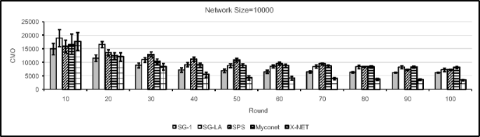
Comparison of different algorithms with X-NET with respect to CMO when network size is 10000
Fig. 29 
Comparison of different algorithms with X-NET with respect to CU when network size is 10000
Fig. 30 
Comparison of different algorithms with X-NET with respect to NSP when network size is 100000
Fig. 31 
Comparison of different algorithms with X-NET with respect to PTO when network size is 100000
Fig. 32 
Comparison of different algorithms with X-NET with respect to CMO when network size is 100000
Fig. 33 
Comparison of different algorithms with X-NET with respect to CU when network size is 100000
- Experiment 3: :
-
This experiment is conducted to study the performance of the proposed algorithm when the distribution of capacities is a uniform distribution. In this experiment the network size is 10000. The results obtained are compared with the results obtained for SG-1, SG-LA, SPS, and Myconet algorithms with respect to NSP, PTO, CMO, and CU. From the results of this experiment given in Figs. 34, 35, 36 and 37 we may conclude that under uniform distribution, the proposed algorithm performs better than other algorithms in terms of NSP and CU.
Fig. 34 
Comparison of different algorithms with X-NET with respect to NSP when uniform distribution is used to generate peers capacities
Fig. 35 
Comparison of different algorithms with X-NET with respect to PTO when uniform distribution is used to generate peers capacities
Fig. 36 
Comparison of different algorithms with X-NET with respect to CMO when uniform distribution is used to generate peers capacities
Fig. 37 
Comparison of different algorithms with X-NET with respect to CU when uniform distribution is used to generate peers capacities
- Experiment 4: :
-
This experiment is conducted to study the impact of catastrophic failure on the performance of the proposed algorithm. For this purpose, we removed different percentages (30 and 60) of super-peers from the network at the beginning of round 30 of the simulation. It should be noted that, the removed peers were added (at the same time of removing peers) to the network as unattached-peers. In this experiment, the network size is 10000 and the power-law distribution is used to generate the capacities of peers. The results obtained are compared with the results obtained for SG-1, SG-LA, SPS, and Myconet algorithms with respect to NSP, PTO, CMO, and CU. From the result of this experiment given in Figs. 38, 39, 40, 41, 42, 43, 44 and 45, we may conclude the following:
-
In terms of NSP and CU, the proposed algorithm performs better than other algorithms under catastrophic failure. The results also have shown, the number of rounds required by the proposed algorithm in order to reach a appropriate configuration after a catastrophic failure is fewer as compared to other algorithms.
Fig. 38 
Comparison of different algorithms with X-NET with respect to NSP when 30 percent of peers are removed
Fig. 39 
Comparison of different algorithms with X-NET with respect to PTO when 30 percent of peers are removed
Fig. 40 
Comparison of different algorithms with X-NET with respect to CMO when 30 percent of peers are removed
Fig. 41 
Comparison of different algorithms with X-NET with respect to CU when 30 percent of peers are removed
Fig. 42 
Comparison of different algorithms with X-NET with respect to NSP when 60 percent of peers are removed
Fig. 43 
Comparison of different algorithms with X-NET with respect to PTO when 60 percent of peers are removed
Fig. 44 
Comparison of different algorithms with X-NET with respect to CMO when 60 percent of peers are removed
Fig. 45 
Comparison of different algorithms with X-NET with respect to CU when 60 percent of peers are removed
-
- Experiment 5: :
-
This experiment is conducted to study the impact of different churn models on the performance of the proposed algorithm. In this experiment, the network size is 10000 and the power-law distribution is used to generate the capacities of the peers. The churn models used in this experiment are described as below.
-
Random churn.1 is designated based on Random churn model reported in [76]. Random churn model has two parameters: joining _probability and leaving _probability. In Random churn.1, joining _probability and leaving _probability parameters are set to 0.7 and 0.3 respectively.
-
Pareto churn.1 is designated based on Pareto churn model reported in [76]. Pareto churn model has two parameters: LifetimeMean and DeadtimeMean. In Pareto churn.1, LifetimeMean and DeadtimeMean parameters are set to 50sec and 20sec respectively.
The results obtained are compared with the results obtained for SG-1, SG-LA, SPS, and Myconet algorithms with respect to NSP, PTO, CMO, and CU. From the result of this experiment given in Figs. 46, 47, 48, 49, 50, 51, 52 and 53, we may conclude the following:
-
In terms of NSP and CU the proposed algorithm performs better than other algorithms.
Fig. 46 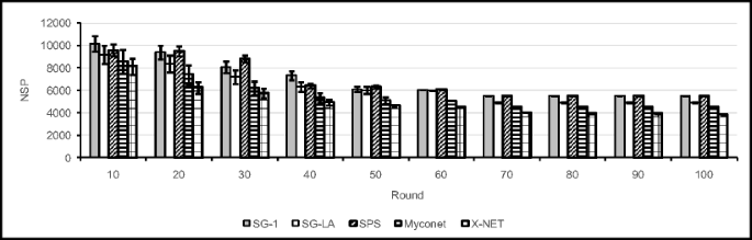
Comparison of different algorithms with X-NET with respect to NSP when Random churn.1 is used
Fig. 47 
Comparison of different algorithms with X-NET with respect to PTO when Random churn.1 is used
Fig. 48 
Comparison of different algorithms with X-NET with respect to CMO when Random churn.1 is used
Fig. 49 
Comparison of different algorithms with X-NET with respect to CU when Random churn.1 is used
Fig. 50 
Comparison of different algorithms with X-NET with respect to NSP when Pareto churn.1 is used
Fig. 51 
Comparison of different algorithms with X-NET with respect to PTO when Pareto churn.1 is used
Fig. 52 
Comparison of different algorithms with X-NET with respect to CMO when Pareto churn.1 is used
Fig. 53 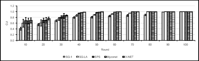
Comparison of different algorithms with X-NET with respect to CU when Pareto churn.1 is used
-
The values CMO and PTO are high at early rounds of operation of the network during which the peers try to gather information about each other for the purpose of searching an appropriate configuration. Higher values for CMO and PTO throughout the operation of the network especially at the early rounds is the price that we need to pay if we want to find a configuration for which NSP attains it lowest possible value and CU attains its highest possible value.
-


7 Conclusion
In this paper, a new dynamic model of CLAs was utilized to design an adaptive algorithm for super-peer selection considering peers capacity. The proposed CLA in which a model of fungal growth is used to adjust the attributes of its cells was used as a mechanism for selection of the super peers in peer-to-peer networks. The proposed super-peer selection algorithm is able to adaptively select super-peers during the operation of the network. To evaluate the proposed algorithm several experiments have been conducted using OverSim simulator. The results of simulation have shown the superiority of the proposed algorithm over the existing algorithms with respect to capacity utilization and number of super-peers.
The proposed algorithm is superior to SG-1, SG-LA, and SPS because it inherits capabilities such as flexibility and resiliency to changes in the environment from fungal growth model. It is also superior to Myconet because it is able to escape from local optima solutions by distributed adaptation capability of the CLA. Note that, Myconet uses a simple fungal growth model and it is not able to escape from local optima solutions. Customizing the proposed super-peer selection algorithm for mobile peer-to-peer networks, designing new algorithms based on the proposed model of CLA for problems such as those reported in [77, 78] may be considered as some of the research lines that can be pursued.
References
Kwok YK (2011) Computing, Peer-to-Peer: Applications, Architecture, Protocols, and challenges. CRC Press, United States
Liang J, Kumar R, Ross K (2004) The kazaa overlay: A measurement study. In: Proceedings of the 19th IEEE annual computer communications workshop, Bonita Springs, Florida, pp 17–20
Kubiatowicz J et al (2000) Oceanstore: An architecture for global-scale persistent storage. In: Proceedings of the ninth international conference on architectural support for programming languages and operating systems, NY, USA, pp 190– 201
Rhea SC, Eaton PR, Geels D, Weatherspoon H, Zhao BY, Kubiatowicz J (2003) Pond: The oceanstore prototype. In: Proceedings of the 2nd USENIX conference on file and storage technologies, CA, USA, vol 3, pp 1–14
Beverly Yang B, Garcia-Molina H (2003) Designing a super-peer network. In: 19th international conference on data engineering, Bangalore, India, pp 49–60
Xu Z, Hu Y (2003) SBARC: A supernode based peer-to-peer file sharing system. In: Proceedings of eighth IEEE international symposium on computers and communication, Antalya, Turkey, pp 1053–1058
Gong L (2001) JXTA: A network programming environment. IEEE Internet Comput 5(3):88–95
Montresor A (2004) A robust protocol for building superpeer overlay topologies. In: Proceedings of the 4th international conference on peer-to-peer computing, Zurich, Switzerland, pp 202–209
Jesi GP, Montresor A, Babaoglu Ö (2006) Proximity-aware superpeer overlay topologies. In: 2nd IEEE international workshop on self-managed networks, systems, and services, Dublin, Ireland, pp 41–50
Xiao L, Zhuang Z, Liu Y (2005) Dynamic layer management in superpeer architectures. IEEE Trans Parallel Distrib Syst 16(11):1078–1091
Snyder PL, Greenstadt R, Valetto G (2009) Myconet: A fungi-inspired model for superpeer-based peer-to-peer overlay topologies. In: Third IEEE international conference on self-adaptive and self-organizing systems, San Francisco, CA, pp 40–50
Gao Z, Gu Z, Wang W (2012) SPSI: A hybrid super-node election method based on information theory. In: 14th international conference on advanced communication technology, Pyeong Chang, pp 1076–1081
Sacha J, Dowling J (2005) A gradient topology for master-slave replication in peer-to-peer environments. In: Proceedings of the international conference on databases, information systems, and peer-to-peer computing, Trondheim, Norway, pp 86–97
Dumitrescu M, Andonie R (2012) Clustering superpeers in p2p networks by growing neural gas. In: 20th euromicro international conference on parallel, distributed and network-based processing, Munich, Germany, pp 311–318
Gholami S, Meybodi M, Saghiri AM (2014) A learning automata-based version of SG-1 protocol for super-Peer selection in peer-to-peer networks. In: Proceedings of the 10th international conference on computing and information technology, Phuket, Thailand, pp 189–201
Liu M, Harjula E, Ylianttila M (2013) An efficient selection algorithm for building a super-peer overlay. J Internet Serv Appl 4(1):1–12
Forestiero A, Mastroianni C, Meo M (2009) Self-Chord: A bio-inspired algorithm for structured P2P systems. In: IEEE/ACM international symposium on cluster computing and the grid, Shanghai, China, pp 44–51
Babaoglu O, Meling H, Montresor A (2002) Anthill: a framework for the development of agent-based peer-to-peer systems. In: 22nd international conference on distributed computing systems, Vienna, Austria, pp 15–22
Ganguly N, Deutsch A (2004) A cellular automata model for immune based search algorithm. In: 6th international conference on cellular automata for research and industry, Amsterdam, Netherlands, pp 142–150
Sharifkhani F, Pakravan MR (2014) Bacterial foraging search in unstructured P2P networks. In: 27th canadian conference on electrical and computer engineering, Toronto, ON, pp 1–8
Singh A, Haahr M (2007) Decentralized clustering in pure p2p overlay networks using schelling’s model. In: IEEE international conference on communications, Glasgow, Scotland, pp 1860–1866
Snyder PL, Giuseppe V (2015) SODAP: Self-organized topology protection for superpeer P2P networks. Scalable Comput: Pract Exper 16(3):271–288
Beigy H, Meybodi M (2004) A mathematical framework for cellular learning automata. Adv Compl Syst 3(4):295–319
Esnaashari M, Meybodi M (2011) A cellular learning automata-based deployment strategy for mobile wireless sensor networks. J Parallel Distrib Comput 71(5):988–1001
Esnaashari M, Meybodi M (2008) A cellular learning automata based clustering algorithm for wireless sensor networks. Sensor Lett 6(5):723–735
Beigy H, Meybodi M (2003) A self-organizing channel assignment algorithm: A cellular learning automata approach. Intell Data Eng Autom Learn 14:119–126
Asnaashari M, Meybodi M (2007) Irregular Cellular Learning Automata and Its Application to Clustering in Sensor Networks. In: Proceedings of 15th conference on electrical engineering, Tehran, Iran, pp 21–28
Zhao Y, Jiang W, Li S, Ma Y, Su G, Lin X (2015) A cellular learning automata based algorithm for detecting community structure in complex networks. Neurocomputing 151:1216–1226
Vahidipour M, Meybodi M, Esnaashari M (2016) Adaptive petri net based on irregular cellular learning automata and its application in vertex coloring problem systems with unknown parameters. Applied Intelligence
Rastegar R, Meybodi M, Hariri A (2006) A new fine-grained evolutionary algorithm based on cellular learning automata. Int J Hybrid Intell Syst 3(2):83–98
Esnaashari M, Meybodi M (2013) Deployment of a mobile wireless sensor network with k-coverage constraint: A cellular learning automata approach. Wirel Netw 19(5):945–968
Saghiri AM, Meybodi M (2016) An approach for designing cognitive engines in cognitive peer-to-peer networks. J Netw Comput Appl 70:17–40
Lo V, Zhou D, Liu Y, GauthierDickey C, Li J (2005) Scalable supernode selection in peer-to-peer overlay networks. In: Hot topics in peer-to-peer systems, DC, USA, 18–25
Irit D, Safra S (2005) On the hardness of approximating minimum vertex cover. Ann Math 162(1):439–485
Rajiv G, Halperin E, Khuller S, Kortsarz G, Srinivasan A (2006) An improved approximation algorithm for vertex cover with hard capacities. J Comput Syst Sci 72(1):16–33
Sachez-Artigas M, Garcia-Lopez P, Skarmeta AFG (2008) On the feasibility of dynamic superpeer ratio maintenance. In: Eighth international conference on peer-to-peer computing, Germany, Aachen, pp 333–342
Min S-H, Holliday J, Cho D-S (2006) Optimal super-peer selection for large-scale p2p system. In: International conference on hybrid information technology, Jeju Island, Korea, vol 2, pp 588–593
Chen J, Wang R-M, Li L, Zhang Z-H, Dong X-S (2013) A distributed dynamic super peer selection method based on evolutionary game for heterogeneous P2P streaming systems. Math Probl Eng 2013
Paweł G, Epema DHJ, Van Steen M (2010) The design and evaluation of a selforganizing superpeer network. IEEE Trans Comput 59(3):317–331
Alexander L, Naumann F, Siberski W, Nejdl W, Thaden U (2004) Semantic overlay clusters within super-peer networks. In: Databases, information systems, and peer-to-peer computing, Berlin, Heidelberg, 33–47
Nejdl W, Wolpers M, Siberski W, Schmitz C, Schlosser M, Brunkhorst I, Löser A (2004) Super-peer-based routing and clustering strategies for RDF-based peer-to-peer networks. Web Semant: Sci, Serv Agents World Wide Web 1(2):177–186
Garbacki P, Epema DHJ, Van Steen M (2007) Optimizing Peer Relationships in a Super-Peer Network. In: 27th international conference on distributed computing systems, Toronto, ON, pp 31–41
Feng W, Liu J, Xiong Y (2008) Stable peers, existence, importance, and application in Peer-To-Peer live video streaming. presented at the the 27th conference on computer communications, AZ, USA, 1364–1372
Sacha J, Dowling J, Cunningham R, Meier R (2006) Using aggregation for adaptive super-peer discovery on the gradient topology. In: Second IEEE international conference on self-managed networks, systems, and services, Dublin, Ireland, pp 73–86
Payberah AH, Dowling J, Haridi S (2011) Glive: The gradient overlay as a market maker for mesh-based p2p live streaming. In: 10th international symposium on parallel and distributed computing. Cluj Napoca, pp 153–162
Fathipour S, Saghiri AM, Meybodi M (2016) An Adaptive Algorithm for Managing Gradient Topology in Peer-to-Peer networks. In: The eight international conference on information and knowledge technology (IKT 2016), Hamedan, Iran
Wolfram S (1986) Theory and applications of cellular automata. World Scientific Publication
Kroc J, Sloot PMA, Georgius Hoekstra A (2010) Simulating complex systems by cellular automata. Understanding Complex Systems. Springer
Somarakis C, Papavassilopoulos G, Udwadia F (2008) A dynamic rule in cellular automata. In: 22nd european conference on modelling and simulation, Nicosia, Cyprus, pp 164–170
Dantchev S (2011) Dynamic neighbourhood cellular automata. Comput J 54(1):26–32
Ilachinski A, Halpern P (1987) Structurally dynamic cellular automata. Complex Syst 1(3):503–527
Cornforth D, Green DG, Newth D (2005) Ordered asynchronous processes in multi-agent systems. Phys D 204:70–82
Bandini S, Bonomi A, Vizzari G (2012) An analysis of different types and effects of asynchronicity in cellular automata update schemes. Nat Comput 11:277–287
Fatès N (2014) Guided tour of asynchronous cellular automata. J Cellular Autom 9:387–416
Barreira-Gonzalez P, Barros J (2016) Configuring the neighbourhood effect in irregular cellular automata based models. Int J Geogr Inf Sci: 1–20
Goles E, Martínez S (2013) Neural and Automata Networks Dynamical Behavior and Applications. Springer Science and Business Media
Li R, Hong Y (2015) On observability of automata networks via computational algebra. In: International conference on language and automata theory and applications, pp 249–262
Narendra KS, Thathachar MAL (1989) Learning automata: An introduction. Prentice-Hall, Englewood Cliffs, NJ
Thathachar M, Sastry PS (2004) Networks of learning automata: Techniques for online stochastic optimization. Kluwer Academic Publishers, Dordrecht, Netherlands
Rezvanian AR, Meybodi M (2015) Finding maximum clique in stochastic graphs using distributed learning automata. Int J Uncertain, Fuzziness Knowl-Based Syst 23(1):1–31
Ghorbani M, Meybodi M, Saghiri AM (2013) A new version of k-random walks algorithm in peer-to-peer networks utilizing learning automata. In: 5th conference on information and knowledge technology, Shiraz, Iran, pp 1–6
Ghorbani M, Meybodi M, Saghiri AM (2013) A novel self-adaptive search algorithm for unstructured peer-to-peer networks utilizing learning automata. In: 3rd joint conference of ai andamp; robotics and 5th robocup iran open international symposium, Qazvin, Iran, pp 1–6
Saghiri AM, Meybodi M (2015) A distributed adaptive landmark clustering algorithm based on mOverlay and learning automata for topology mismatch problem in unstructured peer-to-peer networks. Int J Commun Syst
Saghiri AM, Meybodi M (2015) A self-adaptive algorithm for topology matching in unstructured peer-to-peer networks. J Netw Syst Manag
Beigy H, Meybodi M (2015) A learning Automata-based adaptive uniform fractional guard channel algorithm. J. Supercomput 71(3):871–893
Venkata Krishna P, Misra S, Nagaraju D, Saritha V, Obaidat MS (2016) Learning automata based decision making algorithm for task offloading in mobile cloud. In: International conference on computer, information and telecommunication systems (CITS), Kunming, China, pp 1–6
Beigy H, Meybodi M (2007) Open synchronous cellular learning automata. Adv Complex Syst 10(4):527–556
Beigy H, Meybodi M (2008) Asynchronous cellular learning automata. Automatica 44(5):1350–1357
Beigy H, Meybodi M (2010) Cellular learning automata with multiple learning automata in each cell and its applications. IEEE Trans Syst, Man, Cybern, Part B: Cybern 40(1):54–65
Esnaashari M, Meybodi M (2014) Irregular cellular learning automata. IEEE Trans Cybern 99:1
Mozafari M, Shiri ME, Beigy H (2015) A cooperative learning method based on cellular learning automata and its application in optimization problems. Journal of Computational Science
Saghiri AM, Meybodi M (2017) A closed asynchronous dynamic model of cellular learning automata and its application to peer-to-peer networks. Genet Program Evolvable Mach: 1–37
Robson G, Van West P, Gadd G Exploitation of Fungi. Cambridge University Press
Meškauskas A, Fricker MD, Moore D (2004) Simulating colonial growth of fungi with the Neighbour-Sensing model of hyphal growth. Mycol Res 108(11):1241–1256
Jelasity M, Kowalczyk W, Van Steen M (2003) Newscast computing. Vrije Universiteit Amsterdam, Department of Computer Science, Amsterdam, Netherlands Technical Report IR-CS-006
Baumgart I, Heep B, Krause S (2009) OverSim: A scalable and flexible overlay framework for simulation and real network applications. In: Peer-to-peer computing, Washington, USA, pp 87–88
Villatoro D, Sabater-Mir J, Sen S (2013) Robust convention emergence in social networks through self-reinforcing structures dissolution. ACM Trans Auton Adapt Syst 8(1)
Henri Collet J, Fanchon J (2015) Crystallization and tile separation in the multi-agent systems. Phys A 436:405–417
Author information
Authors and Affiliations
Corresponding author
Rights and permissions
About this article

Cite this article
Saghiri, A.M., Meybodi, M.R. An adaptive super-peer selection algorithm considering peers capacity utilizing asynchronous dynamic cellular learning automata. Appl Intell 48, 271–299 (2018). https://doi.org/10.1007/s10489-017-0946-8
Published:
Issue Date:
DOI: https://doi.org/10.1007/s10489-017-0946-8