Fast convergence to non-isolated minima: four equivalent conditions for ${\textrm{C}^{2}}$ functions

Abstract

Optimization algorithms can see their local convergence rates deteriorate when the Hessian at the optimum is singular. These singularities are inescapable when the optima are non-isolated. Yet, under the right circumstances, several algorithms preserve their favorable rates even when optima form a continuum (e.g., due to over-parameterization). This has been explained under various structural assumptions, including the Polyak–Łojasiewicz condition, Quadratic Growth and the Error Bound. We show that, for cost functions which are twice continuously differentiable ($\textrm{C}^2$), those three (local) properties are equivalent. Moreover, we show they are equivalent to the Morse–Bott property, that is, local minima form differentiable submanifolds, and the Hessian of the cost function is positive definite along its normal directions. We leverage this insight to improve local convergence guarantees for safe-guarded Newton-type methods under any (hence all) of the above assumptions. First, for adaptive cubic regularization, we secure quadratic convergence even with inexact subproblem solvers. Second, for trust-region methods, we argue capture can fail with an exact subproblem solver, then proceed to show linear convergence with an inexact one (Cauchy steps).

1 Introduction

We consider local convergence of algorithms for unconstrained optimization problems

$$\begin{aligned} \min _{x \in \mathcal {M}} f(x), \end{aligned}$$

where $\mathcal {M}$ is a Riemannian manifold¹ and $f:\mathcal {M}\rightarrow {\mathbb R}$ is at least ${\textrm{C}^{1}}$ (continuously differentiable).

When $f$ is ${\textrm{C}^{2}}$ (twice continuously differentiable), the most classical local convergence results ensure favorable rates for standard algorithms provided they converge to a non-singular local minimum $\bar{x}$, that is, one such that the Hessian $\nabla ^2f(\bar{x})$ is positive definite. And indeed, those rates can degrade if the Hessian is merely positive semidefinite. For example, with $f(x) = x^4$, gradient descent (with an appropriate step-size) converges only sublinearly to the minimum, and Newton’s method converges only linearly.

This is problematic if the minimizers of $f$ are not isolated, because in that case the Hessian cannot be positive definite there. This situation arises commonly in applications for structural reasons such as over-parameterization, redundant parameterizations and symmetry—see Sect. 1.2.

Notwithstanding, algorithms often exhibit good local behavior near non-isolated minimizers. As early as the 1960s, this has prompted investigations into properties that such cost functions may satisfy and which lead to fast local rates despite singular Hessians. We study four such properties.

In all that follows, we are concerned with the behavior of algorithms in the vicinity of its local minima. Since we do not assume that they are isolated, rather than selecting one local minimum $\bar{x}$, we select all local minima of the same value. Formally, given a local minimum $\bar{x}$, let

$$\begin{aligned} \mathcal {S}&= \{x \in \mathcal {M}: x {\text { is a local minimum of }} f{\text { and }} f(x) = f_{\mathcal {S}}\} \end{aligned}$$

(1)

denote the set of all local minima with a given value $f_{\mathcal {S}}= f(\bar{x})$.

For $f$ of class ${\textrm{C}^{2}}$, it is particularly favorable if $\mathcal {S}$ is a differentiable submanifold of $\mathcal {M}$ around $\bar{x}$. In that case the set $\mathcal {S}$ has a tangent space $\textrm{T}_{\bar{x}}\mathcal {S}$ at $\bar{x}$. It is easy to see that each vector $v \in \textrm{T}_{\bar{x}}\mathcal {S}$ must be in the kernel of the Hessian $\nabla ^2f$ at $\bar{x}$ because the gradient $\nabla f$ is constant (zero) on $\mathcal {S}$. Thus, $\textrm{T}_{\bar{x}}\mathcal {S}\subseteq \ker \nabla ^2f(\bar{x})$. Since $\bar{x}$ is a local minimum, we also know that $\nabla ^2f(\bar{x})$ is positive semidefinite. Then, in the spirit of asking the Hessian to be “as positive definite as possible”, the best we can hope for is that the kernel of $\nabla ^2f(\bar{x})$ is exactly $\textrm{T}_{\bar{x}}\mathcal {S}$, in which case the restriction of $\nabla ^2f(\bar{x})$ to the normal space $\textrm{N}_{\bar{x}}\mathcal {S}$, that is, the orthogonal complement of $\textrm{T}_{\bar{x}}\mathcal {S}$ in $\textrm{T}_{\bar{x}}\mathcal {M}$, is positive definite.

We call this the Morse–Bott property (MB), and we write $\mu$-MB to indicate that the positive eigenvalues are at least $\mu > 0$. The definition requires $f$ to be twice differentiable.

Definition 1.1

Let $\bar{x}$ be a local minimum of $f$ with associated set $\mathcal {S}$ (1). We say $f$ satisfies the Morse–Bott property at $\bar{x}$ if

If also $\langle v, \nabla ^2f(\bar{x})[v]\rangle \ge \mu \Vert v\Vert ^2$ for some $\mu > 0$ and all $v \in \textrm{N}_{\bar{x}}\mathcal {S}$ then we say $f$ satisfies $\mu$-MB at $\bar{x}$.

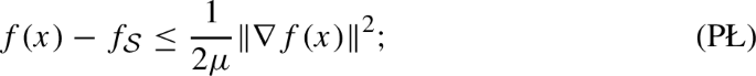
At first, a reasonable objection to the above is that one may not want to assume that $\mathcal {S}$ is a submanifold. Perhaps for that reason, it is far more common to encounter other assumptions in the optimization literature. We focus on three: Polyak–Łojasiewicz (PŁ), error bound (EB) and quadratic growth (QG). The first goes back to the 1960s [81]. The latter two go back at least to the 1990s [22, 70].

Below, the first two definitions (as stated) require $f$ to be differentiable. The distance to a set is defined as usual: ${{\,\textrm{dist}\,}}(x, \mathcal {S}) = \inf _{y\in \mathcal {S}} {{\,\textrm{dist}\,}}(x, y)$ where ${{\,\textrm{dist}\,}}(x, y)$ is the Riemannian distance on $\mathcal {M}$.

Definition 1.2

Let $\bar{x}$ be a local minimum of $f$ with associated set $\mathcal {S}$ (1). We say $f$ satisfies

• the Polyak–Łojasiewicz condition with constant $\mu > 0$ ($\mu$-PŁ) around $\bar{x}$ if

  

• the error bound with constant $\mu > 0$ ($\mu$-EB) around $\bar{x}$ if

  

• quadratic growth with constant $\mu > 0$ ($\mu$-QG) around $\bar{x}$ if

  

all understood to hold for all x in some neighborhood of $\bar{x}$.

Note that all the definitions are local around a point $\bar{x}$. Two observations are immediate: (i) QG implies that $\bar{x}$ is a strict minimum relatively to $\mathcal {S}$ (1), meaning that $f(x) > f_{\mathcal {S}}$ for all $x \notin \mathcal {S}$ close enough to $\bar{x}$, and (ii) both EB and PŁ imply that critical points and $\mathcal {S}$ coincide around $\bar{x}$. Thus, both EB and PŁ rule out existence of saddle points near $\bar{x}$. By extension, we say that $f$ satisfies any of these four properties around a set of local minima if it holds around each point of that set.

1.1 Contributions

A number of relationships between PŁ, EB and QG are well known already for $f$ of class ${\textrm{C}^{1}}$: see Table 1 and Sect. 1.3. Our first main contribution in this paper is to show that:

If f is of class ${\textrm{C}^{2}}$, then PŁ, EB, QG and MB are essentially equivalent.

Here, “essentially” means that the constant $\mu$ may degrade (arbitrarily little) and the neighborhoods where properties hold may shrink. Notably, we show that if f is ${\textrm{C}^{p}}$ with $p \ge 2$, then PŁ, EB and QG all imply that the set of local minima $\mathcal {S}$ is locally smooth (at least ${\textrm{C}^{p - 1}}$). We also give counter-examples when $f$ is only ${\textrm{C}^{1}}$. Explicitly, in Sect. 2 we summarize known results for $f$ of class ${\textrm{C}^{1}}$ and we contribute the following:

Table 1 Summary of implications

• Theorem 2.16 shows PŁ around $\bar{x}$ implies $\mathcal {S}$ is a ${\textrm{C}^{p - 1}}$ submanifold around $\bar{x}$ if f is ${\textrm{C}^{p}}$ with $p \ge 2$. Remark 2.19 provides counter-examples if $f$ is only ${\textrm{C}^{1}}$. If $f$ is analytic, so is $\mathcal {S}$, as already shown by Feehan [44].

• Lemma 2.14 is instrumental to prove Theorem 2.16 and to analyze algorithms. It states that under PŁ the gradient locally aligns with the dominant eigenvectors of the Hessian.

• Corollary 2.17 deduces that $\mu$-PŁ implies $\mu$-MB if $f$ is ${\textrm{C}^{2}}$.

• Proposition 2.8 shows $\mu$-QG implies $\mu '$-EB with $\mu '<\mu$ arbitrarily close if $f$ is ${\textrm{C}^{2}}$. Remark 2.9 provides a counter-example if $f$ is only ${\textrm{C}^{1}}$.

• Proposition 2.4 shows $\mu$-EB implies $\mu '$-PŁ with $\mu '<\mu$ arbitrarily close if $f$ is ${\textrm{C}^{2}}$. If $f$ is only ${\textrm{C}^{1}}$ with L-Lipschitz continuous $\nabla f$, Karimi et al. [52] showed the same with $\mu ' = \mu ^2/L$.

In Sect. 4, we study the classical globalized versions of Newton’s method. We strengthen their local convergence guarantees when minimizers are not isolated but the ${\textrm{C}^{2}}$ cost function satisfies any (hence all) of the above. The key observation that enables those improvements is the fact that we may use all four conditions in the analysis without loss of generality. Specifically:

• Cubic regularization enjoys superlinear convergence under PŁ, as shown by Nesterov and Polyak [76]. Yue et al. [97] further showed quadratic convergence under EB. Both references assume an exact subproblem solver. Leveraging our results above, we show that quadratic convergence still holds with inexact subproblem solvers (Theorem 4.1).

• For the trust-region method with exact subproblem solver, we were surprised to find that even basic capture-type convergence properties can fail in the presence of non-isolated local minima (Sect. 4.2). Notwithstanding, common implementations of the trust-region method use a truncated conjugate gradient (tCG) subproblem solver, and those do, empirically, exhibit superlinear convergence under the favorable conditions discussed above. We discuss this further in Remark 4.14, and we show a partial result in Theorem 4.9, namely, that using the Cauchy step (i.e., the first iterate of tCG) yields linear convergence.

As is classical, to prove the latter results, we rely on capture theorems and Lyapunov stability. Those hold under assumptions of vanishing step-sizes and bounded path length. In Sect. 3, we state those building blocks succinctly, adapted to accommodate non-isolated local minima.

1.2 Non-isolated minima in applications

We now illustrate how optimization problems with continuous sets of minima occur in applications.

Fig. 1

Optimization through the map $\varphi$

In all three scenarios below, we can cast the cost function $f:\mathcal {M}\rightarrow {\mathbb R}$ as a composition of some other function $g:\mathcal {N}\rightarrow {\mathbb R}$ through a map $\varphi :\mathcal {M}\rightarrow \mathcal {N}$, where $\mathcal {N}$ is a smooth manifold (see Fig. 1 and [60]). If $g$ and $\varphi$ are twice differentiable, then the Morse–Bott property (MB) for $f= g\circ \varphi$ can come about as follows. Consider a local minimum ${\bar{y}}$ for $g$. The set $\mathfrak {X}= \varphi ^{-1}({\bar{y}})$ consists of local minima for $f$. Pick a point $\bar{x}\in \mathfrak {X}$. Assume $x \mapsto {{\,\textrm{rank}\,}}\textrm{D}\varphi (x)$ is constant in a neighborhood of $\bar{x}$. Then, the set $\mathfrak {X}$ is an embedded submanifold of $\mathcal {M}$ around $\bar{x}$ with tangent space $\ker \textrm{D}\varphi (\bar{x})$. Moreover, the Hessians of $f$ and $g$ at $\bar{x}$ are related by

$$\begin{aligned} \nabla ^2f(\bar{x}) = \textrm{D}\varphi (\bar{x})^* \circ \nabla ^2g(\varphi (\bar{x})) \circ \textrm{D}\varphi (\bar{x}). \end{aligned}$$

(2)

Therefore, if $\nabla ^2g(\varphi (\bar{x}))$ is positive definite, then $\ker \nabla ^2f(\bar{x}) = \textrm{T}_{\bar{x}}\mathfrak {X}$ and $\nabla ^2f(\bar{x})$ is positive definite along the orthogonal complement. In other words: $f$ satisfies the Morse–Bott property (MB) at $\bar{x}$. We present below a few concrete examples of optimization problems where this can happen.

Over-parameterization and nonlinear regression. Consider minimizing $f(x) = \frac{1}{2} \Vert F(x) - b\Vert ^2$ with $F :{\mathbb R}^m \rightarrow {\mathbb R}^n$ a ${\textrm{C}^{2}}$ function. We cast this as above with $g(y) = \frac{1}{2} \Vert y - b\Vert ^2$ and $\varphi = F$. Suppose $\mathfrak {X}= \varphi ^{-1}(b) = \{x: F(x) = b\}$ is non-empty (interpolation regime), which is typical in deep learning. This is the set of global minimizers of f. If ${{\,\textrm{rank}\,}}\textrm{D}F(x)$ is equal to a constant r in a neighborhood of $\mathfrak {X}$, then $\mathfrak {X}$ is a smooth submanifold of ${\mathbb R}^m$ of dimension $m - r$. If additionally the problem is over-parameterized, that is, $m > n \ge r$, then $\mathfrak {X}$ has positive dimension (see Fig. 2 for an illustration). The discussion above immediately implies that $f$ satisfies MB on $\mathfrak {X}$. See also Nesterov and Polyak [76, §4.2] who argue that PŁ holds in this setting.

Fig. 2

(Left) Submanifold of minima where MB holds. (Middle) A ${\textrm{C}^{1}}$ function that satisfies QG but not PŁ nor EB. (Right) A ${\textrm{C}^{1}}$ function that satisfies PŁ, yet whose set of minima is a cross

Redundant parameterizations and submersions. Say we want to minimize $g:\mathcal {N}\rightarrow {\mathbb R}$ constrained to ${\mathcal {C}} \subseteq \mathcal {N}$. If ${\mathcal {C}}$ is complicated, and if we have access to a parameterization $\varphi$ for that set (so that $\varphi (\mathcal {M}) = {\mathcal {C}}$), it may be advantageous to minimize $f= g\circ \varphi$ instead. If the parameterization is redundant, this can cause $f$ to have non-isolated minima, even if the minima of $g$ are isolated.

As an example, consider minimizing $g:{\mathbb R}^{m \times n} \rightarrow {\mathbb R}$ over the bounded-rank matrices ${\mathcal {C}} = \{Y \in {\mathbb R}^{m \times n}: {{\,\textrm{rank}\,}}Y \le r\}$. A popular approach consists in lifting the search space to $\mathcal {M}= {\mathbb R}^{m \times r} \times {\mathbb R}^{n \times r}$ and minimizing $f= g\circ \varphi$, where $\varphi :\mathcal {M}\rightarrow \mathcal {N}$ is defined as $\varphi (L, R) = LR^\top$. The parameterization is redundant because $\varphi (LJ^{-1}, RJ^{\top }) = \varphi (L, R)$ for all invertible J. In particular, given a local minimum $Y \in {\mathcal {C}}$ of $g$, the fiber $\varphi ^{-1}(Y)$ is unbounded, which hinders convergence analyses (see [59]). However, if Y is of maximal rank r then $\textrm{D}\varphi$ has constant rank in a neighborhood of $\varphi ^{-1}(Y)$. From the discussion above, it follows that $f$ satisfies MB on $\varphi ^{-1}(Y)$ if the (Riemannian) Hessian of g (restricted to the manifold of rank-r matrices) is positive definite.

Similarly, Burer and Monteiro [25, 26] introduced a popular approach to minimize a function $g$ over the set of positive semidefinite matrices of bounded rank through the map $\varphi :Y \mapsto YY^\top$. The resulting function $f= g\circ \varphi$ can have non-isolated minima. However, the same arguments as above ensure that MB holds at minimizers of maximal rank when $g$ is strongly convex (this setting is for example considered in [103]). This further extends to tensors [63].

Symmetries and quotients. Some optimization problems have intrinsic symmetries. For example, in estimation problems, if the measurements are invariant under particular transformations of the signal, then the signal can only be retrieved up to those transformations. The likelihood function then has symmetries, and possibly a continuous set of optima as a result. Sometimes, factoring these symmetries out (that is, passing to the quotient) yields a quotient manifold, and we can investigate optimization on that manifold [4]. In the notation of our general framework above, $\varphi$ is then the quotient map. In particular, $\varphi$ is a submersion, so that if ${\bar{y}} \in \mathcal {N}$ is a non-singular minimum of $g$ then $f$ satisfies MB on $\varphi ^{-1}({\bar{y}})$ (which is a submanifold of dimension $\dim \mathcal {M}- \dim \mathcal {N}$). See also [24, §9.9] for the case where $\mathcal {N}$ is a Riemannian quotient of $\mathcal {M}$.

1.3 Related work

Historical note. Discussions about convergence to singular minima appear in the literature at least as early as [82, §6.1]. Luo and Tseng [70] introduced the EB condition explicitly to study gradient methods around singular minima. The QG property is arguably as old as optimization, though the earliest work we could locate is by Bonnans and Ioffe [22]. They employed QG to understand complicated landscapes with non-isolated minima. Łojasiewicz [68, 69] introduced his inequalities and used them subsequently to analyze gradient flow trajectories. Specifically, he proved that for analytic functions the trajectories either converge to a point or diverge. Concurrently, Polyak [81] introduced what became known as the Polyak–Łojasiewicz (PŁ) variant (also “gradient dominance”) to study both gradient flows and discrete gradient methods. Later, Kurdyka [55] developed generalizations now known as Kurdyka–Łojasiewicz (KŁ) inequalities. They are satisfied by most functions encountered in practice, as discussed in [9, §4]. In contrast, the Morse–Bott property has received little attention in the optimization literature. Early work by Shapiro [87] analyzes perturbations of optimization problems assuming a property similar to MB. There is also a mention of gradient flow under MB in [49, Prop. 12.3].

Relationships between properties. Several articles have explored the interplay between MB, PŁ, EB and QG in the last decades. The implication PŁ $\Rightarrow$ QG has a rich history. It can be obtained as a corollary from [50, Basic lemma] (based on Ekeland’s variational principle; see also [41, Lem. 2.5]). It also follows from Łojasiewicz-type arguments that consist in bounding the length of gradient flow trajectories [79, Prop. 1]. Likewise, Bolte et al. [19] study growth under KŁ inequalities, with PŁ $\Rightarrow$ QG as a special case. For lower-semicontinuous functions, Corvellec and Motreanu [35, Thm. 4.2] show that $\mu$-EB $\Rightarrow$ $\mu$-QG. They also find that $\mu$-QG $\Rightarrow$ $\frac{\mu }{2}$-EB for convex functions [35, Prop. 5.3]. In a somewhat different setting, Drusvyatskiy et al. [40, Cor. 3.2] prove that $\mu$-EB $\Rightarrow$ $\mu '$-QG with arbitrary $\mu ' < \mu$. With extra assumptions, they also show $\mu$-QG $\Rightarrow$ $\mu '$-EB but without control of $\mu '$. Later, Bolte et al. [21] proved an equivalence between KŁ inequalities and function growth for convex and potentially non-smooth functions. Their results seem to generalize to semi-convex functions. See also [100] and [39] for equivalences between EB and QG. Karimi et al. [52] established implications between several properties encountered in the optimization literature. In particular, they also show that PŁ and EB are equivalent, and that they both imply QG. Liao et al. [65] extended this to a non-smooth and weakly convex setting. Li and Pong [62] showed that EB implies PŁ for non-smooth functions under a level set separation assumption, though with no control on the PŁ constant. Implications between PŁ and EB are also reported in [42, Thm. 3.7, Prop. 3.8] for non-smooth functions under broad conditions. In the context of functional analysis, Feehan [44] proved that MB and PŁ are equivalent for analytic functions defined on Banach spaces. The work of [94, Ex. 2.9] also mentions that MB implies PŁ for ${\textrm{C}^{2}}$ functions. A more general implication is given by Arbel and Mairal [8, Prop. 1] for parameterized optimization problems. Previously, Bonnans and Ioffe [22] had exhibited sufficient conditions (similar to MB) for QG to hold. As a side note, Marteau-Ferey et al. [71] proved that MB is a sufficient condition to ensure that a non-negative function is globally decomposable as a sum of squares of smooth functions.

Convergence guarantees. The error bound approach of Luo and Tseng [70] has proven to be fruitful as multiple analyses based on this condition followed. Notably, Tseng [91] proved local superlinear convergence rates for some Newton-type methods applied to systems of nonlinear equations. They relied specifically on EB and did not assume isolated minima. Later, Yamashita and Fukushima [96] employed EB to establish capture theorems and quadratic convergence rates for the Levenberg–Marquardt method. Fan and Yuan [43], Behling et al. [12] and Boos et al. [23] generalized their results (in particular to solutions with a non-zero residual). More recently, Bellavia and Morini [14] found that two adaptive regularized methods converge quadratically for nonlinear least-squares problems (assuming that EB holds).

An early work of Anitescu [6] combines the QG property with other conditions to ensure isolated minima in constrained optimization, then deducing convergence results. Later, QG has found applications mainly in the context of convex optimization: see [67] for coordinate descent, [75] for various gradient methods, and [39] for the proximal gradient method. It is also worth mentioning that the definition of QG does not require differentiability of the function. For this reason, QG is valuable to study algorithms in non-smooth optimization too [36, 61].

The literature about convergence results based on Łojasiewicz inequalities is vast, and we touch here on some particularly relevant references. Absil et al. [2] discretized the arguments from [69] and obtained capture results for a broad class of optimization algorithms. Lageman [56, 57] provided generalizations to broader classes of functions. Later, such arguments have been used in many contexts to prove algorithmic convergence guarantees, among which [9, 20] are particularly influential works. Moreover, Attouch et al. [10] proposed a general abstract framework based on KŁ to derive capture results and convergence rates, and Frankel et al. [46] extended their statements. See also [74] for a framework that encompasses higher-order methods. Li and Pong [62] studied the preservation of Łojasiewicz inequalities under function transformations (such as sums and compositions). See also [11, 90] for the preservation of PŁ through function compositions. Interestingly, the PŁ condition is known to be a necessary condition for gradient descent to converge linearly [1, Thm. 5]. Recently, Yue et al. [98] proved that acceleration is impossible to minimize globally PŁ functions: gradient descent is optimal absent further structure. Assuming PŁ, Stonyakin et al. [88] formulated stopping criteria for gradient methods when the gradient is corrupted with noise. Using KŁ inequalities, Noll and Rondepierre [78] and Khanh et al. [53] analyzed the convergence of line-search gradient descent and trust-region methods. Łojasiewicz inequalities have also proved relevant for the study of second-order algorithms and superlinear convergence rates. A prominent example is the regularized Newton algorithm that converges superlinearly when PŁ holds, as shown in [76]. More recently, Zhou et al. [105], Yue et al. [97] provided finer analyses of this algorithm, respectively assuming Łojasiewicz inequalities and EB. Qian and Pan [84] extended the abstract framework of Attouch et al. [10] to establish superlinear convergence rates.

Stochastic algorithms have also been extensively studied through Łojasiewicz inequalities, and we briefly mention a few references here. Dereich and Kassing [37, 38] analyzed stochastic gradient descent (SGD) in the presence of non-isolated minima, using Łojasiewicz inequalities among other things. Local analyses of SGD using PŁ inequalities are given by Li et al. [64] and Wojtowytsch [94]. Ko and Li [54] studied the local stability and convergence of SGD in the presence of a compact set of minima with a condition that is weaker than PŁ. As for second-order algorithms, Masiha et al. [72] proved that a stochastic version of regularized Newton has fast convergence under PŁ.

Łojasiewicz inequalities are also particularly suited to analyze the convergence of flows. Notably, Łojasiewicz [69] bounded the path length of gradient flow trajectories and Polyak [81] derived linear convergence of flows assuming PŁ. Related results for flows but under MB are claimed in [49, Prop. 12.3]. More recently, Apidopoulos et al. [7] considered the Heavy-Ball differential equation and deduced convergence guarantees from PŁ. Wojtowytsch [95] studied a continuous model for SGD and the impact of the noise on the trajectory.

Finally, we found only few convergence results based on MB in the optimization literature. Fehrman et al. [45] derive capture theorems and asymptotic sublinear convergence rates for gradient descent assuming that MB holds on the set of minima. They also provide probabilistic bounds for stochastic variants. Usevich et al. [92] consider optimization problems over unitary matrices. They propose sufficient conditions for MB to hold at a local optimum and then exploit the induced PŁ condition to obtain convergence rates. In order to solve systems of nonlinear equations, Zeng [99] proposes a Newton-type method that is robust to non-isolated solutions. It enjoys local quadratic convergence assuming a MB-type property. The algorithm requires the knowledge of the dimension of the set of solutions.

Applications. Non-isolated minima arise in all sorts of optimization problems. It is common for non-convex inverse problems to have continuous symmetries, hence non-isolated minima (see [104]). In the context of deep learning, Cooper [34] proved that the set of global minima of a sufficiently over-parameterized neural network is a smooth manifold. In the last decade, there has been a renewed interest in Łojasiewicz inequalities because they are compatible with these complicated non-convex landscapes. In particular, a whole line of research exploits them to understand deep learning problems specifically. As an example, Oymak and Soltanolkotabi [80] employed PŁ to analyze the path taken by (stochastic) gradient descent in the vicinity of minimizers. Several other works suggested that non-convex machine learning loss landscapes can be understood in over-parameterized regimes through the lens of Łojasiewicz inequalities [11, 13, 66, 90]. Specifically, they argue that PŁ holds on a significant part of the search space and analyze (stochastic) gradient methods. Chatterjee [30] also establishes local convergence results for a large class of neural networks with PŁ inequalities.

1.4 Notation and geometric preliminaries

Table 2 Simplifications in the case where $\mathcal {M}$ is a Euclidean space

This section anchors notation and some basic geometric facts. In the important case where $\mathcal {M}= {\mathbb R}^n$, several objects reduce as summarized in Table 2.

We let $\langle \cdot , \cdot \rangle$ denote the inner product on $\textrm{T}_x\mathcal {M}$—it may depend on $x \in \mathcal {M}$, but the base point is always clear from context. The associated norm is $\Vert v\Vert = \sqrt{\langle v, v\rangle }$. The map ${{\,\textrm{dist}\,}}:\mathcal {M}\times \mathcal {M}\rightarrow {\mathbb R}_+$ is the Riemannian distance on $\mathcal {M}$. We let $\textrm{B}(x, \delta )$ denote the open ball of radius $\delta$ around $x \in \mathcal {M}$. The tangent bundle is $\textrm{T}\mathcal {M}= \{ (x, v): x \in \mathcal {M}\text { and } v \in \textrm{T}_x\mathcal {M}\}$.

Moving away from $x \in \mathcal {M}$ along the geodesic with (sufficiently small) initial velocity $v \in \textrm{T}_x\mathcal {M}$ for unit time produces the point $\textrm{Exp}_x(v) \in \mathcal {M}$ (Riemannian exponential). The injectivity radius at x is $\textrm{inj}(x) > 0$. It is defined such that, given $y \in \textrm{B}(x, \textrm{inj}(x))$, there exists a unique smallest vector $v \in \textrm{T}_x\mathcal {M}$ for which $\textrm{Exp}_x(v) = y$. We denote this v by $\textrm{Log}_x(y)$ (Riemannian logarithm). Additionally, given $x \in \mathcal {M}$ and $y \in \textrm{B}(x, \textrm{inj}(x))$, we let $\Gamma _{x}^{y} :\textrm{T}_x\mathcal {M}\rightarrow \textrm{T}_y\mathcal {M}$ denote parallel transport along the unique minimizing geodesic between x and y. If $v = \textrm{Log}_x(y)$, we also let $\Gamma _{v} = \Gamma _{x}^{y}$.

Let $\mathfrak {X}$ be a subset of $\mathcal {M}$. We need the notions of tangent and normal cones to $\mathfrak {X}$, defined below.

Definition 1.3

The tangent cone to a set $\mathfrak {X}$ at $x \in \mathfrak {X}$ is the closed set

$$\begin{aligned} \textrm{T}_x\mathfrak {X}= \left\{ \lim _{k \rightarrow +\infty }\frac{1}{t_k}\textrm{Log}_x(x_k) \,\Big |\, x_k \in \mathfrak {X}, t_k > 0 {\text { for all }}k, x_k \rightarrow x, t_k \rightarrow 0 \right\} . \end{aligned}$$

We also let $\textrm{N}_x\mathfrak {X}= \big \{w \in \textrm{T}_x\mathcal {M}: \langle w, v\rangle \le 0 {\text { for all }}v \in \textrm{T}_x\mathfrak {X}\big \}$ denote the normal cone to $\mathfrak {X}$ at x.

When $\mathfrak {X}$ is a submanifold of $\mathcal {M}$ around x, the cones $\textrm{T}_x\mathfrak {X}$ and $\textrm{N}_x\mathfrak {X}$ reduce to the tangent and normal spaces of $\mathfrak {X}$ at x. (By “submanifold”, we always mean embedded submanifold.)

Given $x \in \mathcal {M}$, we let ${{\,\textrm{dist}\,}}(x, \mathfrak {X}) = \inf _{y \in \mathfrak {X}} {{\,\textrm{dist}\,}}(x, y)$ denote the distance of x to $\mathfrak {X}$. We further let ${{\,\textrm{proj}\,}}_\mathfrak {X}(x)$ denote the set of minima of the optimization problem $\min _{y \in \mathfrak {X}} \,{{\,\textrm{dist}\,}}(x, y)$. If this set is non-empty (which is the case in particular if $\mathfrak {X}$ is closed), then we have:

$$\begin{aligned} \forall \bar{x}\in \mathfrak {X}, y \in {{\,\textrm{proj}\,}}_\mathfrak {X}(x), & {{\,\textrm{dist}\,}}(y, \bar{x}) \le 2 {{\,\textrm{dist}\,}}(x, \bar{x}). \end{aligned}$$

(3)

Indeed, the triangle inequality yields ${{\,\textrm{dist}\,}}(y, \bar{x}) \le {{\,\textrm{dist}\,}}(x, y) + {{\,\textrm{dist}\,}}(x, \bar{x})$, and ${{\,\textrm{dist}\,}}(x, y) = {{\,\textrm{dist}\,}}(x, \mathfrak {X}) \le {{\,\textrm{dist}\,}}(x, \bar{x})$. Moreover, if $y \in {{\,\textrm{proj}\,}}_\mathfrak {X}(x)$ with ${{\,\textrm{dist}\,}}(x, y) < \textrm{inj}(y)$ then $\textrm{Log}_y(x) \in \textrm{N}_y\mathfrak {X}$.

The set of local minima $\mathcal {S}$ defined in (1) may not be closed: consider for example the function $f(x) = \textrm{sgn}(x)\exp (-\frac{1}{x^2})(1 + \sin (\frac{1}{x^2}))$ with $f_{\mathcal {S}}= 0$. It follows that the projection onto $\mathcal {S}$ may be empty. Notwithstanding, the following holds:

Lemma 1.4

Around each $\bar{x}\in \mathcal {S}$ there exists a neighborhood in which ${{\,\textrm{proj}\,}}_\mathcal {S}$ is non-empty.

Proof

Let ${\mathcal {U}}$ be an open neighborhood of $\bar{x}$ such that $f(x) \ge f_{\mathcal {S}}$ for all $x \in {\mathcal {U}}$. Let ${\mathcal {V}}_1, {\mathcal {V}}_2 \subset {\mathcal {U}}$ be two closed balls around $\bar{x}$ of radii $\delta > 0$ and $\frac{1}{4}\delta$ respectively. Then $\mathcal {S}\cap {\mathcal {V}}_1 = f^{-1}(f_{\mathcal {S}}) \cap {\mathcal {V}}_1$, showing that $\mathcal {S}\cap {\mathcal {V}}_1$ is closed and the projection onto this set is non-empty. Let $x \in {\mathcal {V}}_2$ and $y \in {{\,\textrm{proj}\,}}_{\mathcal {S}\cap {\mathcal {V}}_1}(x)$. Then ${{\,\textrm{dist}\,}}(x, y) \le \frac{1}{4}\delta$. Moreover, for all $y' \in \mathcal {S}{\setminus } {\mathcal {V}}_1$ we have ${{\,\textrm{dist}\,}}(x, y') \ge \frac{3}{4}\delta$. It follows that ${{\,\textrm{proj}\,}}_{\mathcal {S}}(x) = {{\,\textrm{proj}\,}}_{\mathcal {S}\cap {\mathcal {V}}_1}(x)$, and this is non-empty. $\square$

From these considerations we deduce that the projection onto $\mathcal {S}$ is always locally well behaved.

Lemma 1.5

Let $\bar{x}\in \mathcal {S}$. There exists a neighborhood ${\mathcal {U}}$ of $\bar{x}$ such that for all $x \in {\mathcal {U}}$ the set ${{\,\textrm{proj}\,}}_{\mathcal {S}}(x)$ is non-empty, and for all $y \in {{\,\textrm{proj}\,}}_{\mathcal {S}}(x)$ we have ${{\,\textrm{dist}\,}}(x, y) < \textrm{inj}(y)$. In particular, $v = \textrm{Log}_y(x)$ is well defined and $v \in \textrm{N}_y\mathcal {S}$.

Proof

Let ${\mathcal {U}}$ be a neighborhood of $\bar{x}$ where ${{\,\textrm{proj}\,}}_{\mathcal {S}}$ is non-empty (given by Lemma 1.4). Given ${\bar{\delta }} < \textrm{inj}(\bar{x})$, the ball ${\bar{\textrm{B}}}(\bar{x}, \delta )$ is compact for all $\delta < {\bar{\delta }}$. Define $h(\delta ) = \inf _{x \in {\bar{\textrm{B}}}(\bar{x}, 2\delta )} \textrm{inj}(x)$ on the interval . The function h is continuous with $h(0) = \textrm{inj}(\bar{x}) > 0$ so we can pick $\delta > 0$ such that $\delta \le h(\delta )$. Let $x \in \textrm{B}(\bar{x}, \delta ) \cap {\mathcal {U}}$ and $y \in {{\,\textrm{proj}\,}}_\mathcal {S}(x)$. By definition of the projection we have ${{\,\textrm{dist}\,}}(x, y) \le {{\,\textrm{dist}\,}}(x, \bar{x}) < \delta$. Moreover, inequality (3) yields ${{\,\textrm{dist}\,}}(y, \bar{x}) \le 2 {{\,\textrm{dist}\,}}(x, \bar{x}) \le 2\delta$ so $h(\delta ) \le \textrm{inj}(y)$. It follows that ${{\,\textrm{dist}\,}}(x, y) < \delta \le h(\delta ) \le \textrm{inj}(y)$ and $v = \textrm{Log}_{y}(x)$ is well defined. The fact that v is in the normal cone follows from optimality conditions of projections. $\square$

Given a self-adjoint linear map H, we let $\lambda _i(H)$ denote the ith largest eigenvalue of H, and $\lambda _{\min }(H)$ and $\lambda _{\max }(H)$ denote the minimum and maximum eigenvalues respectively.

2 Four equivalent properties

In this section, we establish that MB, PŁ, EB and QG (see Definitions 1.1 and 1.2) are equivalent around a local minimum $\bar{x}$ when $f$ is ${\textrm{C}^{2}}$. Specifically, we show the implication graph in Fig. 3.

Fig. 3

Implication graph when $f$ is ${\textrm{C}^{2}}$. The main missing pieces were PŁ $\Rightarrow$ MB and QG $\Rightarrow$ EB, both secured with the right constants and under the right regularity assumptions

It is well known that PŁ implies QG around minima: see references in Sect. 1.3. Perhaps the most popular argument relies on the bounded length of gradient flow trajectories under the more general Łojasiewicz inequality [2, 19, 68, 69, 79].

Definition 2.1

Let $\bar{x}$ be a local minimum of $f$ with associated set $\mathcal {S}$ (1). We say $f$ satisfies the Łojasiewicz inequality with constants and $\mu > 0$ around $\bar{x}$ if

for all x in some neighborhood of $\bar{x}$.

Notice that if $f$ is Łojasiewicz with exponent $\theta$ then it is Łojasiewicz with exponent $\theta '$ for all $\theta \le \theta ' < 1$ (though possibly in a different neighborhood). The case $\theta = \frac{1}{2}$ is exactly the (PŁ) condition.

Proposition 2.2

(${\text {P}{\L } }\Rightarrow {\text {QG}}$) Suppose that $f$ satisfies (Ł) around $\bar{x}\in \mathcal {S}$. Then $f$ satisfies

$$\begin{aligned} f(x) - f_{\mathcal {S}}\ge \big ((1 - \theta )\sqrt{2\mu }\big )^{\frac{1}{1 - \theta }}{{\,\textrm{dist}\,}}(x, \mathcal {S})^{\frac{1}{1 - \theta }} \end{aligned}$$

for all x sufficiently close to $\bar{x}$. In particular, if $\theta = \frac{1}{2}$, this shows $\mu$-(PŁ) $\Rightarrow$ $\mu$-(QG).

We include a classical proof in Appendix A for completeness, with care regarding neighborhoods.

2.1 Two straightforward implications

In this section we show that ${\text {MB}} \Rightarrow {\text {QG}}$ and ${\text {EB}}\Rightarrow {\text {P}{\L } }$. These implications are known and direct. We give succinct proofs for completeness. The first one follows immediately from a Taylor expansion.

Proposition 2.3

(${\text {MB}} \Rightarrow {\text {QG}}$) Suppose that $f$ is ${\textrm{C}^{2}}$ and satisfies $\mu$-(MB) at $\bar{x}\in \mathcal {S}$. Then $f$ satisfies $\mu '$-(QG) around $\bar{x}$ for all $\mu ' < \mu$.

Proof

Let ${\mathcal {U}}$ be a neighborhood of $\bar{x}$ as in Lemma 1.5. Let $d$ be the codimension of $\mathcal {S}$ (around $\bar{x}$). Given $\mu ' < \mu$, pick and shrink ${\mathcal {U}}$ so that for all $x \in {\mathcal {U}}$ and $y \in {{\,\textrm{proj}\,}}_\mathcal {S}(x)$ we have $\lambda _{d}(\nabla ^2f(y)) \ge \mu ' + \varepsilon$. Given $x \in {\mathcal {U}}$ and $y \in {{\,\textrm{proj}\,}}_\mathcal {S}(x)$, a Taylor expansion around y gives

$$\begin{aligned} f(x) - f_{\mathcal {S}}= \frac{1}{2}\langle v, \nabla ^2f(y)[v]\rangle + o(\Vert v\Vert ^2) \ge \frac{\mu ' + \varepsilon }{2} {{\,\textrm{dist}\,}}(x, \mathcal {S})^2 + o({{\,\textrm{dist}\,}}(x, \mathcal {S})^2), \end{aligned}$$

where $v = \textrm{Log}_y(x)$ is normal to $\mathcal {S}$. We get the inequality $\mu '$-(QG) for all x sufficiently close to $\bar{x}$. $\square$

Proposition 2.4

(${\text {EB}} \Rightarrow {\text {P}{\L } }$) Suppose that $f$ is ${\textrm{C}^{2}}$ and satisfies $\mu$-(EB) around $\bar{x}\in \mathcal {S}$. Then $f$ satisfies $\mu '$-(PŁ) around $\bar{x}$ for all $\mu ' < \mu$.

Proof

Let ${\mathcal {U}}$ be the intersection of two neighborhoods of $\bar{x}$: one where $\mu$-(EB) holds, and the other provided by Lemma 1.5. Given $x \in {\mathcal {U}}$ and $y \in {{\,\textrm{proj}\,}}_{\mathcal {S}}(x)$, a Taylor expansion around y yields

$$\begin{aligned} f(x) - f_{\mathcal {S}}= \frac{1}{2}\langle v, \nabla ^2f(y)[v]\rangle + o(\Vert v\Vert ^2) & {\text {and}} & \nabla f(x) = \Gamma _{v} \nabla ^2f(y)[v] + o(\Vert v\Vert ), \end{aligned}$$

where $v = \textrm{Log}_y(x)$. Using the Cauchy–Schwarz inequality and the triangle inequality, it follows that

$$\begin{aligned} f(x) - f_{\mathcal {S}}\le \frac{1}{2}\Vert v\Vert \Vert \nabla ^2f(y)[v]\Vert + o(\Vert v\Vert ^2) \le \frac{1}{2}\Vert v\Vert \Vert \nabla f(x)\Vert + o(\Vert v\Vert ^2). \end{aligned}$$

Finally, EB gives that $\Vert v\Vert \le \frac{1}{\mu } \Vert \nabla f(x)\Vert$ so $f(x) - f_{\mathcal {S}}\le \frac{1}{2\mu }\Vert \nabla f(x)\Vert ^2 + o(\Vert \nabla f(x)\Vert ^2)$. We get the inequality $\mu '$-(PŁ) for all x sufficiently close to $\bar{x}$. $\square$

Remark 2.5

Suppose that $f$ is only ${\textrm{C}^{1}}$ and $\nabla f$ is locally L-Lipschitz continuous around $\bar{x}$. If $\mu$-EB holds around $\bar{x}$ then $f$ satisfies PŁ with constant $\frac{\mu ^2}{L}$ around $\bar{x}$ [52, Thm. 2]. (This still holds locally on manifolds with the same proof.) The constant worsens but that is inevitable: see the example in Remark 2.19.

2.2 Quadratic growth implies error bound

In this section, we show that QG implies EB for ${\textrm{C}^{2}}$ functions. Other works proving this implication either assume that $f$ is convex (see [35, Prop. 5.3], [52], and [39, Cor. 3.6]) or do not provide control on the constants (see [40, Cor. 3.2]). For this, we first characterize a distance growth rate when we move from $\mathcal {S}$ in a normal direction (see Definition 1.3). Recall that for now $\mathcal {S}$ is not necessarily smooth, and therefore $\textrm{N}_{\bar{x}} \mathcal {S}$ is a priori only a cone.

Lemma 2.6

Let $\bar{x}\in \mathcal {S}$ and $v \in \textrm{N}_{\bar{x}}\mathcal {S}$ unitary. Then ${{\,\textrm{dist}\,}}(\textrm{Exp}_{\bar{x}}(tv), \mathcal {S}) = t + o(t)$ as $t \rightarrow 0$, $t \ge 0$.

Proof

Let ${\mathcal {U}}$ be a neighborhood of $\bar{x}$ as in Lemma 1.5. Shrink ${\mathcal {U}}$ so that for all $x \in {\mathcal {U}}$ and $y \in {{\,\textrm{proj}\,}}_{\mathcal {S}}(x)$ we have ${{\,\textrm{dist}\,}}(y, \bar{x}) < \textrm{inj}(\bar{x})$. Given a small parameter $t > 0$, define $x(t) = \textrm{Exp}_{\bar{x}}(tv)$ and let $y(t) \in {{\,\textrm{proj}\,}}_{\mathcal {S}}(x(t))$. From (3) we have ${{\,\textrm{dist}\,}}(y(t), \bar{x}) \le 2t$, and it follows that $y(t) \rightarrow \bar{x}$ as $t \rightarrow 0$. Define $u(t) = \textrm{Log}_{y(t)}(x(t))$ and $w(t) = \textrm{Log}_{\bar{x}}(y(t))$. Then

$$\begin{aligned} {{\,\textrm{dist}\,}}(x(t), \mathcal {S})^2 = \Vert u(t)\Vert ^2 = \Vert tv - w(t) + \Gamma _{y(t)}^{\bar{x}}u(t) - tv + w(t)\Vert ^2 = \Vert tv - w(t)\Vert ^2 + o(t^2) \end{aligned}$$

as $t \rightarrow 0$ because $\Vert \Gamma _{y(t)}^{\bar{x}}u(t) - tv + w(t)\Vert = o(t)$ as $t \rightarrow 0$ [89, Eq. (6)]. In particular, for all t sufficiently small we have

$$\begin{aligned} {{\,\textrm{dist}\,}}(x(t), \mathcal {S})^2 = t^2 - 2t\langle w(t), v\rangle + \Vert w(t)\Vert ^2 + o(t^2) \ge t^2 - 2t\langle w(t), v\rangle + o(t^2). \end{aligned}$$

Let $I \subseteq {\mathbb R}_{> 0}$ be the times when $y(t) \ne \bar{x}$. If $\inf I > 0$ then the final claim holds because $y(t) = \bar{x}$ for small enough t. Suppose now that $\inf I = 0$. Define $r(t) = \frac{w(t)}{\Vert w(t)\Vert }$ on I, and let ${\mathcal {A}}$ be the set of accumulation points of r(t) as $t \rightarrow 0$, $t \in I$. Then ${\mathcal {A}}$ is included in the unit sphere and ${\mathcal {A}} \subseteq \textrm{T}_{\bar{x}}\mathcal {S}$ by definition. Given $a \in {\mathcal {A}}$ and $t \in I$, we can use $\langle a, v\rangle \le 0$ to find that

$$\begin{aligned} {{\,\textrm{dist}\,}}(x(t), \mathcal {S})^2 \ge t^2 - 2 t \Vert w(t)\Vert \langle r(t) - a + a, v\rangle + o(t^2) \ge t^2 - 4 t^2 \Vert r(t) - a\Vert + o(t^2). \end{aligned}$$

It follows that ${{\,\textrm{dist}\,}}(x(t), \mathcal {S})^2 \ge t^2 - 4 t^2 {{\,\textrm{dist}\,}}(r(t), {\mathcal {A}}) + o(t^2) = t^2 + o(t^2)$ because ${{\,\textrm{dist}\,}}(r(t), {\mathcal {A}}) \rightarrow 0$ as $t \rightarrow 0$. $\square$

Using this rate, we now find that QG implies the following bounds for $\nabla ^2f$ in the normal cones of $\mathcal {S}$. Note that the following proposition does not yet show QG $\Rightarrow$ MB, because to establish MB we still need to argue that $\mathcal {S}$ is a smooth set.

Proposition 2.7

Suppose $f$ is ${\textrm{C}^{2}}$ and satisfies (QG) with constant $\mu$ around $\bar{x}\in \mathcal {S}$. Then for all $y \in \mathcal {S}$ sufficiently close to $\bar{x}$ and all $v \in \textrm{N}_{y}\mathcal {S}$ we have

$$\begin{aligned} \langle v, \nabla ^2f(y)[v]\rangle \ge \mu \Vert v\Vert ^2 & {\text {and}} & \Vert \nabla ^2f(y)[v]\Vert \ge \mu \Vert v\Vert . \end{aligned}$$

Proof

Let ${\mathcal {U}}$ be an open neighborhood of $\bar{x}$ where $\mu$-QG holds. Let $y \in \mathcal {S}\cap {\mathcal {U}}$ and $v \in \textrm{N}_{y}\mathcal {S}$. For all small enough $t > 0$, we obtain from a Taylor expansion that

$$\begin{aligned} f(\textrm{Exp}_y(tv)) - f_{\mathcal {S}}&= \frac{t^2}{2}\langle v, \nabla ^2f(y)[v]\rangle + o(t^2) \ge \frac{\mu }{2} {{\,\textrm{dist}\,}}(\textrm{Exp}_y(tv), \mathcal {S})^2 \\&= \frac{\mu }{2}t^2\Vert v\Vert ^2 + o(t^2), \end{aligned}$$

where the inequality comes from QG and the following equality comes from Lemma 2.6. Take $t \rightarrow 0$ to get the first inequality. The other inequality follows by Cauchy–Schwarz. $\square$

We deduce from this that, under QG, the gradient norm is locally bounded from below and from above by the distance to $\mathcal {S}$, up to some constant factors. This notably secures EB.

Proposition 2.8

(${\text {QG}} \Rightarrow {\text {EB}}$) Suppose $f$ is ${\textrm{C}^{2}}$ and satisfies $\mu$-(QG) around $\bar{x}\in \mathcal {S}$. For all $\mu ^\flat < \mu$ and $\lambda ^\sharp > \lambda _{\max }(\nabla ^2f(\bar{x}))$ there exists a neighborhood ${\mathcal {U}}$ of $\bar{x}$ such that for all $x \in {\mathcal {U}}$ we have

$$\begin{aligned} \mu ^\flat {{\,\textrm{dist}\,}}(x, \mathcal {S}) \le \Vert \nabla f(x)\Vert \le \lambda ^\sharp {{\,\textrm{dist}\,}}(x, \mathcal {S}). \end{aligned}$$

Proof

Let ${\mathcal {U}}$ be a neighborhood of $\bar{x}$ as in Lemma 1.5. Shrink ${\mathcal {U}}$ so that for all $x \in {\mathcal {U}}$ and $y \in {{\,\textrm{proj}\,}}_\mathcal {S}(x)$ the inequalities of Proposition 2.7 hold. Now let $x \in {\mathcal {U}}$ and $y \in {{\,\textrm{proj}\,}}_\mathcal {S}(x)$. Define $v = \textrm{Log}_y(x)$ and $\gamma (t) = \textrm{Exp}_y(tv)$, so that $y = \gamma (0)$ and $x = \gamma (1)$. Then a Taylor expansion of $\nabla f$ around y yields

$$\begin{aligned}&\quad \Gamma _{v}^{-1} \nabla f(x) = \nabla ^2f(y)[v] + r(x) {\text {where}}\\&\quad r(x) = \int _0^1 \Big ( \Gamma _{\tau v}^{-1} \circ \nabla ^2f(\gamma (\tau )) \circ \Gamma _{\tau v} - \nabla ^2f(y) \Big )[v] \textrm{d}\tau . \end{aligned}$$

The Hessian is continuous so $r(x) = o(\Vert v\Vert )$ as $x \rightarrow \bar{x}$. Moreover, Proposition 2.7 provides that $\Vert \nabla ^2f(y)[v]\Vert \ge \mu \Vert v\Vert$ so using the triangle inequality and the reverse triangle inequality we get

$$\begin{aligned} \Vert v\Vert \big (\mu - o(1)\big ) \le \Vert \nabla f(x)\Vert \le \Vert v\Vert \big (\lambda _{\max }(\nabla ^2f(y)) + o(1)\big ) \end{aligned}$$

as $x \rightarrow \bar{x}$. We get the result if we choose x close enough to $\bar{x}$. $\square$

The first inequality in the previous proposition is exactly EB. In Proposition 2.4 we showed that EB implies PŁ when $f$ is ${\textrm{C}^{2}}$. Thus, it also holds that QG implies PŁ.

Remark 2.9

When $f$ is only ${\textrm{C}^{1}}$ it is not true that QG implies EB or PŁ. To see this, consider the function $f(x) = 2x^2 + x^2\sin (1/\sqrt{|x|})$ (see Fig. 2). It is ${\textrm{C}^{1}}$ and satisfies QG around the minimum $\bar{x}= 0$ because $f(x) \ge x^2$. However, there are other local minima arbitrarily close to ${{\bar{x}}}$. Those are critical points with function value strictly larger than $f(\bar{x})$, which disqualifies EB and PŁ around $\bar{x}$.

Remark 2.10

Combining Propositions 2.2 and 2.8 ($\mu$-PŁ $\Rightarrow$ $\mu$-QG and $\mu$-QG $\Rightarrow$ $\mu '$-EB), one finds that $\mu$-PŁ implies $\mu '$-EB for ${\textrm{C}^{2}}$ functions. In fact, Karimi et al. [52] show that $\mu$-PŁ implies $\mu$-EB for ${\textrm{C}^{1}}$ functions, globally so if PŁ holds globally. Indeed, for x sufficiently close to $\bar{x}$, we have

$$\begin{aligned} \frac{\mu }{2}{{\,\textrm{dist}\,}}(x, \mathcal {S})^2 \le f(x) - f_{\mathcal {S}}\le \frac{1}{2\mu }\Vert \nabla f(x)\Vert ^2, \end{aligned}$$

where the second inequality comes from PŁ, and the first inequality is QG (implied by PŁ).

Combining all previous implications, we obtain that MB implies PŁ. This is also straightforward from Taylor expansion arguments.

Corollary 2.11

(${\text {MB}} \Rightarrow {\text {P}{\L } }$) Suppose that $f$ is ${\textrm{C}^{2}}$ and satisfies $\mu$-(MB) at $\bar{x}\in \mathcal {S}$. Let $0< \mu ' < \mu$. Then $f$ satisfies $\mu '$-(PŁ) around $\bar{x}$.

As a consequence, if $f$ is $\mu$-MB on any subset of $\mathcal {S}$ then for all $\mu ' < \mu$ there exists a neighborhood of that subset where $f$ is $\mu '$-PŁ. When $f$ is ${\textrm{C}^{3}}$ the size of the neighborhood where PŁ holds can be controlled (to some extent) with the third derivative. A version of this corollary appears in [94, Ex. 2.9] with a different trade-off between control of the neighborhood and the constant $\mu '$. Feehan [44, Thm. 6] shows a similar result in Banach spaces assuming that the function is ${\textrm{C}^{3}}$.

2.3 PL implies a smooth set of minima and MB

The MB property is explicitly strong because it presupposes a smooth set of minima, and it clearly implies PŁ, EB, and QG. It raises a natural question: do the latter also enforce some structure on the set of minima? In this section we show that the answer is yes for ${\textrm{C}^{2}}$ functions: if PŁ (or EB or QG) holds around $\bar{x}\in \mathcal {S}$ then $\mathcal {S}$ must be a submanifold around $\bar{x}$.

To get a sense of why $\mathcal {S}$ cannot have singularities, suppose that $\mathcal {M}= {\mathbb R}^2$ and that around $\bar{x}$ the set of minima is the union of two orthogonal lines (a cross) that intersect at $\bar{x}$. Then it must be that $\nabla ^2f(\bar{x}) = 0$ because the gradient is zero along both lines. However, if we assume PŁ then the spectrum of $\nabla ^2f(x)$ must contain at least one positive eigenvalue bigger than $\mu$ for all points $x \in \mathcal {S}{\setminus } \{\bar{x}\}$ close to $\bar{x}$, owing to the QG property. We obtain a contradiction because the eigenvalues of $\nabla ^2f$ are continuous.

To generalize this intuition, we first show that PŁ induces a lower-bound on the positive eigenvalues of $\nabla ^2f$.

Proposition 2.12

Suppose $f$ is ${\textrm{C}^{2}}$ and $\mu$-(PŁ) around $\bar{x}\in \mathcal {S}$. If $\lambda$ is a non-zero eigenvalue of $\nabla ^2f(\bar{x})$ then $\lambda \ge \mu$.

Proof

Let $\lambda > 0$ be an eigenvalue of $\nabla ^2f(\bar{x})$ with associated unit eigenvector v. Then

$$\begin{aligned} f(\textrm{Exp}_{\bar{x}}(tv)) - f_{\mathcal {S}}= \frac{\lambda }{2}t^2 + o(t^2) & {\text {and}} & \nabla f(\textrm{Exp}_{\bar{x}}(tv)) = \lambda t \Gamma _{tv} v + o(t). \end{aligned}$$

The PŁ condition implies $\frac{\lambda }{2}t^2 + o(t^2) \le \frac{1}{2\mu }{\lambda ^2 t^2 + o(t^2)}$, which gives the result as $t \rightarrow 0$. $\square$

The latter argument is inconclusive when $\lambda = 0$. Still, we do get control of the Hessian’s rank.

Corollary 2.13

Suppose $f$ is ${\textrm{C}^{2}}$ and $\mu$-(PŁ) around $\bar{x}\in \mathcal {S}$. Then ${{\,\textrm{rank}\,}}(\nabla ^2f(x)) = {{\,\textrm{rank}\,}}(\nabla ^2f(\bar{x}))$ for all $x \in \mathcal {S}$ close enough to $\bar{x}$.

Proof

Since $f$ is ${\textrm{C}^{2}}$ the eigenvalues of $\nabla ^2f$ are continuous and the map $x \mapsto {{\,\textrm{rank}\,}}(\nabla ^2f(x))$ is lower semi-continuous, that is, if $x \in \mathcal {M}$ is close enough to $\bar{x}$ then ${{\,\textrm{rank}\,}}\nabla ^2f(x) \ge d$, where $d= {{\,\textrm{rank}\,}}\nabla ^2f(\bar{x})$. Furthermore, if $y \in \mathcal {S}$ is sufficiently close to $\bar{x}$ then $\lambda _{d+ 1}(\nabla ^2f(y)) < \mu$ by continuity of eigenvalues, and Proposition 2.12 then implies $\lambda _{d+ 1}(\nabla ^2f(y)) = 0$. $\square$

This allows us to show that $\nabla f$ aligns locally in a special way with the eigenspaces of $\nabla ^2f$. This alignment will be particularly valuable to analyze second-order algorithms in Sect. 4.

Lemma 2.14

Suppose $f$ is ${\textrm{C}^{2}}$ and satisfies (PŁ) around $\bar{x}\in \mathcal {S}$. Let $d= {{\,\textrm{rank}\,}}(\nabla ^2f(\bar{x}))$. Then the orthogonal projector P(x) onto the top $d$ eigenspace of $\nabla ^2f(x)$ is well defined when x is sufficiently close to $\bar{x}$, and (with I denoting identity)

$$\begin{aligned} \Vert (I - P(x)) \nabla f(x)\Vert = o({{\,\textrm{dist}\,}}(x, \mathcal {S})) = o(\Vert \nabla f(x)\Vert ) \end{aligned}$$

as $x \rightarrow \bar{x}$. Additionally, if $\nabla ^2f$ is locally Lipschitz continuous around $\bar{x}$ then $\Vert (I - P(x)) \nabla f(x)\Vert = O({{\,\textrm{dist}\,}}(x, \mathcal {S})^2) = O(\Vert \nabla f(x)\Vert ^2)$ as $x \rightarrow \bar{x}$.

Proof

Given a point $x \in \mathcal {M}$, let $P(x) :\textrm{T}_x\mathcal {M}\rightarrow \textrm{T}_x\mathcal {M}$ denote the orthogonal projector onto the top $d$ eigenspace of $\nabla ^2f(x)$. This is well defined provided $\lambda _{d}(\nabla ^2f(x)) > \lambda _{d+1}(\nabla ^2f(x))$. Let ${\mathcal {U}}$ be a neighborhood of $\bar{x}$ as in Lemma 1.5. By continuity of the eigenvalues of $\nabla ^2f$, we can shrink ${\mathcal {U}}$ so that for all $x \in {\mathcal {U}}$ and $y \in {{\,\textrm{proj}\,}}_\mathcal {S}(x)$ the projectors P(x) and P(y) are well defined. Given $x \in {\mathcal {U}}$, we let $y \in {{\,\textrm{proj}\,}}_\mathcal {S}(x)$ and $v = \textrm{Log}_{y}(x)$. Now define $\gamma (t) = \textrm{Exp}_y(tv)$. A Taylor expansion of the gradient around y gives that

$$\begin{aligned} \nabla f(x)&= \Gamma _{v} \big (\nabla ^2f(y)[v] + r(x)\big ) {\text {where}} r(x) \\&= \int _0^1 \big ( \Gamma _{\tau v}^{-1} \circ \nabla ^2f(\gamma (\tau )) \circ \Gamma _{\tau v} - \nabla ^2f(y) \big )[v] \textrm{d}\tau . \end{aligned}$$

By Corollary 2.13, the rank of $\nabla ^2f$ is locally constant on $\mathcal {S}$ (equal to $d$) so $\nabla ^2f(y) = P(y) \nabla ^2f(y)$ whenever x is sufficiently close to $\bar{x}$ (using the bound ${{\,\textrm{dist}\,}}(y, \bar{x}) \le 2 {{\,\textrm{dist}\,}}(x, \bar{x})$ from (3)). It follows that

$$\begin{aligned} (I - P(x)) \nabla f(x)&= (I - P(x)) \Gamma _{v} \big (P(y) \nabla ^2f(y)[v] + r(x)\big ). \end{aligned}$$

Notice that $\Gamma _{v} \rightarrow I$ as $x \rightarrow \bar{x}$ and $P(y) \rightarrow P(\bar{x})$ as $x \rightarrow \bar{x}$ so $(I - P(x))\Gamma _{v} P(y) \rightarrow 0$ as $x \rightarrow \bar{x}$. It follows that $(I - P(x)) \nabla f(x) = o(\Vert v\Vert )$ as $x \rightarrow \bar{x}$. The claim follows by noting that $\Vert v\Vert = {{\,\textrm{dist}\,}}(x, \mathcal {S})$ and the fact that ${{\,\textrm{dist}\,}}(x, \mathcal {S})$ is commensurate $\Vert \nabla f(x)\Vert$ (as shown in Proposition 2.8).

Suppose now that $\nabla ^2f$ is locally Lipschitz continuous around $\bar{x}$. Then P is also locally Lipschitz continuous around $\bar{x}$ [93, Thm. 1] and $(I - P(x)) \Gamma _{v} P(y) = (I - P(x)) \Gamma _{v} (P(y) - \Gamma _{v}^{-1} P(x)) = O(\Vert v\Vert )$. Moreover, we have $r(x) = O(\Vert v\Vert ^2)$ so it follows that $(I - P(x)) \nabla f(x) = O(\Vert v\Vert ^2)$ as $x \rightarrow \bar{x}$. We conclude again with Proposition 2.8. $\square$

The lemma below exhibits a submanifold $\mathcal {Z}$ that contains $\bar{x}$. It need not coincide with the set of minima $\mathcal {S}$. However, they do coincide if we assume that PŁ holds. This is the main argument to show that $\mathcal {S}$ is locally a submanifold whenever $f$ is PŁ and sufficiently regular.

Lemma 2.15

Suppose $f$ is ${\textrm{C}^{p}}$ with $p \ge 2$. Let $\bar{x}\in \mathcal {S}$ and define ${\mathcal {U}} = \{x \in \mathcal {M}: {{\,\textrm{dist}\,}}(x, \bar{x}) < \textrm{inj}(\bar{x})\}$. Let $P(\bar{x})$ denote the orthogonal projector onto the image of $\nabla ^2f(\bar{x})$. Then the set

$$\begin{aligned} \mathcal {Z}= \{x \in {\mathcal {U}} : P(\bar{x}) \Gamma _{x}^{\bar{x}} \nabla f(x) = 0\} \end{aligned}$$

is a ${\textrm{C}^{p - 1}}$ embedded submanifold locally around $\bar{x}$. If $f$ is analytic then $\mathcal {Z}$ is also analytic.

Proof

We build a local defining function for $\mathcal {Z}$. Let $d$ be the rank of $\nabla ^2f(\bar{x})$ and $u_1, \ldots , u_d$ be a set of orthonormal eigenvectors of $\nabla ^2f(\bar{x})$ with associated eigenvalues $\lambda _1, \ldots , \lambda _d> 0$. We define $h :{\mathcal {U}} \rightarrow {\mathbb R}^d$ as $h_i(x) = \langle u_i, \Gamma _{x}^{\bar{x}} \nabla f(x)\rangle$. Clearly, $h(x) = 0$ if and only if $x \in \mathcal {Z}$. The function h is ${\textrm{C}^{p - 1}}$ if $f$ is ${\textrm{C}^{p}}$, and analytic if $f$ is analytic. For all $\dot{x} \in \textrm{T}_{\bar{x}}\mathcal {M}$ we have

$$\begin{aligned} \textrm{D}h_i(\bar{x})[\dot{x}] = \langle u_i, \nabla ^2f(\bar{x})[\dot{x}]\rangle = \langle \nabla ^2f(\bar{x})[u_i], \dot{x}\rangle = \lambda _i\langle u_i, \dot{x}\rangle . \end{aligned}$$

It follows that $\textrm{D}h(\bar{x})$ has full rank. Thus, $\mathcal {Z}$ is a submanifold around $\bar{x}$ with the stated regularity. $\square$

A result similar to Lemma 2.15 is presented in [31, Lem. 1] for Banach spaces. We are now ready for one of our main theorems, regarding the regularity of the set of local minimizers $\mathcal {S}$ (1).

Theorem 2.16

Suppose $f$ is ${\textrm{C}^{p}}$ with $p \ge 2$ and satisfies (PŁ) around $\bar{x}\in \mathcal {S}$. Then $\mathcal {S}$ is a ${\textrm{C}^{p - 1}}$ submanifold of $\mathcal {M}$ locally around $\bar{x}$. If $f$ is analytic then $\mathcal {S}$ is also analytic.

Proof

We let $d$ denote the rank of $\nabla ^2f(\bar{x})$. By Corollary 2.13, ${{\,\textrm{rank}\,}}\nabla ^2f(y) = d$ for all $y \in \mathcal {S}$ sufficiently close to $\bar{x}$. We let ${\mathcal {U}} \subseteq \textrm{B}(\bar{x}, \textrm{inj}(\bar{x}))$ be a neighborhood of $\bar{x}$ such that for all $x \in {\mathcal {U}}$ the orthogonal projector $P(x) :\textrm{T}_x\mathcal {M}\rightarrow \textrm{T}_x\mathcal {M}$ onto the top $d$ eigenspace of $\nabla ^2f(x)$ is well defined (it exists because eigenvalues of $\nabla ^2f$ are continuous). Lemma 2.15 ensures that

$$\begin{aligned} \mathcal {Z}= \{x \in {\mathcal {U}} : P(\bar{x}) \Gamma _{x}^{\bar{x}} \nabla f(x) = 0\} \end{aligned}$$

is a submanifold around $\bar{x}$. Clearly, $\mathcal {S}\cap {\mathcal {U}} \subseteq \mathcal {Z}$ holds. We now show the other inclusion to obtain that $\mathcal {S}$ and $\mathcal {Z}$ coincide around $\bar{x}$. From Lemma 2.14 we have $\Vert \nabla f(x)\Vert \le \Vert P(x) \nabla f(x)\Vert + o(\Vert \nabla f(x)\Vert )$ as $x \rightarrow \bar{x}$. Moreover, the triangle inequality gives $\Vert P(x) \nabla f(x)\Vert \le \Vert (P(x) - \Gamma _{\bar{x}}^{x} P(\bar{x}) \Gamma _{x}^{\bar{x}}) \nabla f(x)\Vert + \Vert P(\bar{x}) \Gamma _{x}^{\bar{x}} \nabla f(x)\Vert$. By continuity of P we have $P(x) - \Gamma _{\bar{x}}^{x} P(\bar{x}) \Gamma _{x}^{\bar{x}} = o(1)$ as $x \rightarrow \bar{x}$ so it follows that

$$\begin{aligned} \Vert \nabla f(x)\Vert \le \Vert P(\bar{x}) \Gamma _{x}^{\bar{x}} \nabla f(x)\Vert + o(\Vert \nabla f(x)\Vert ) \end{aligned}$$

as $x \rightarrow \bar{x}$. We conclude that $P(\bar{x}) \Gamma _{x}^{\bar{x}} \nabla f(x) = 0$ implies $\nabla f(x) = 0$ for all x sufficiently close to $\bar{x}$. This confirms that $\mathcal {Z}\subseteq \mathcal {S}\cap {\mathcal {U}}$ around $\bar{x}$ because all critical points near $\bar{x}$ are in $\mathcal {S}$ by PŁ. $\square$

The codimension of $\mathcal {S}$ is equal to the rank of $\nabla ^2f$ on $\mathcal {S}$, as expected. A similar result holds for Banach spaces when the function is assumed analytic [44, Thm. 1]. Around $\bar{x}$, the set of all minima of $f$ and $\mathcal {S}$ coincide when PŁ holds. Hence, Theorem 2.16 implies that the set of minima of $f$ is a submanifold around $\bar{x}$. Using the QG property we now deduce that PŁ implies MB.

Corollary 2.17

If $f$ is ${\textrm{C}^{2}}$ and $\mu$-(PŁ) around $\bar{x}\in \mathcal {S}$ then it satisfies $\mu$-(MB) at $\bar{x}$. The same holds if $f$ is $\mu$-(EB) or $\mu$-(QG) rather than $\mu$-(PŁ).

Proof

Apply Theorem 2.16 to get that $\mathcal {S}$ is locally a ${\textrm{C}^{1}}$ submanifold around $\bar{x}$. Proposition 2.2 gives (QG) around $\bar{x}$. Finally apply Proposition 2.7 to normal eigenvectors of $\nabla ^2f(\bar{x})$. This yields that the normal eigenvalues are at least $\mu$. We obtain the same result if we suppose $\mu$-EB or $\mu$-QG instead of $\mu$-PŁ. This is because they both imply $\mu '$-PŁ for $\mu ' < \mu$ arbitrarily close to $\mu$. Taking the limit $\mu ' \rightarrow \mu$ gives $\mu$-MB. $\square$

Remark 2.18

(Connections to the distance function) Given a closed set $\mathfrak {X}\subseteq \mathcal {M}$, the function $f(x) = \frac{1}{2}{{\,\textrm{dist}\,}}_{\mathfrak {X}}(x)^2$ clearly satisfies QG. If $f$ is ${\textrm{C}^{p}}$ with $p \ge 2$ in a neighborhood of $\mathfrak {X}$ then Theorem 2.16 applies, revealing that $\mathfrak {X}$ is a ${\textrm{C}^{p-1}}$ submanifold. This question is of independent interest, see for example [15] for a proof when assuming $p \ge 3$.

Remark 2.19

(Structure when $f$ is only ${\textrm{C}^{1}}$) Theorem 2.16 requires $f$ to be ${\textrm{C}^{2}}$. And indeed, if $f$ is only ${\textrm{C}^{1}}$ the set of minima may not be a submanifold. We provide two examples.

The function $f(x, y) = \frac{x^2y^2}{x^2 + y^2}$ is ${\textrm{C}^{1}}$ and PŁ around the origin, yet its minimizers form a cross (see Fig. 2).² Incidentally, f is $\frac{1}{\sqrt{2}}$-EB but only $\frac{1}{2}$-PŁ around the origin, confirming that the constant worsens for the implication ${\text {EB}} \Rightarrow {\text {P}{\L } }$ when $f$ is only ${\textrm{C}^{1}}$.

Additionally, let $\mathfrak {X}\subseteq \mathcal {M}$ be a closed set and suppose that the distance function ${{\,\textrm{dist}\,}}_{\mathfrak {X}}$ is ${\textrm{C}^{1}}$ around $\mathfrak {X}$ (such a set is called proximally smooth [32]). For $f(x) = \frac{1}{2}{{\,\textrm{dist}\,}}_\mathfrak {X}(x)^2$, we find that $\nabla f(x) = x - {{\,\textrm{proj}\,}}_\mathfrak {X}(x)$, meaning that $f$ is PŁ around $\mathfrak {X}$ with constant $\mu = 1$. This holds in particular for all closed convex sets, yet many such sets fail to be ${\textrm{C}^{0}}$ submanifolds (e.g., consider a closed square in $\mathcal {M}= {\mathbb R}^2$). This provides further examples of ${\textrm{C}^{1}}$ functions satisfying PŁ yet for which the set of minima is not ${\textrm{C}^{0}}$.

Remark 2.20

(Restricted secant inequality) It is possible to show equivalences with even more properties. For example, as in [101], we say $f$ satisfies the restricted secant inequality (RSI) with constant $\mu$ around $\bar{x}\in \mathcal {S}$ if $\langle \nabla f(x), v\rangle \ge \mu {{\,\textrm{dist}\,}}(x, \mathcal {S})^2$ for all x in a neighborhood of $\bar{x}$, where $v = -\textrm{Log}_x(y)$ and $y \in {{\,\textrm{proj}\,}}_\mathcal {S}(x)$. From simple Taylor expansion arguments, we find that $\mu$-MB implies $\mu '$-RSI for all $\mu ' < \mu$. By Cauchy–Schwarz, we also find that $\mu$-RSI implies $\mu$-EB for ${\textrm{C}^{1}}$ functions (see [52]). It follows that for ${\textrm{C}^{2}}$ functions RSI is also equivalent to the four properties that we consider.

Remark 2.21

(Other Łojasiewicz exponents) The PŁ condition is exactly (Ł) with exponent $\theta = \frac{1}{2}$. We comment here about other values of $\theta$. First, suppose $f$ is ${\textrm{C}^{1}}$ and $\nabla f$ locally Lipschitz continuous. If $f$ is non-constant around $\bar{x}\in \mathcal {S}$ then it cannot satisfy (Ł) with an exponent $\theta < \frac{1}{2}$ around $\bar{x}$. This is because these assumptions are incompatible with the growth property from Proposition 2.2. See also [1, Thm. 4] for an algorithmic perspective on this. Now suppose $f$ is ${\textrm{C}^{2}}$ and satisfies (Ł) with exponent $\theta$ around $\bar{x}\in \mathcal {S}$. If and $\nabla ^2f$ is Lipschitz continuous around $\bar{x}$ then PŁ holds around $\bar{x}$. Furthermore, if $\theta = \frac{2}{3}$ and $f$ is additionally ${\textrm{C}^{3}}$ then PŁ also holds around $\bar{x}$. We include a proof of these observations in Appendix B.

3 Stability of minima and linear rates

In this section, we consider two types of algorithmic questions: the stability of minima and standard local convergence rates. We review some necessary classical arguments, taking this opportunity to generalize some of them to accommodate non-isolated minima. This will serve us well to analyze algorithms in Sect. 4.

3.1 Capture for sets of non-isolated minima

Typically, global convergence analyses of optimization algorithms merely guarantee that iterates accumulate only at critical points. The set of accumulation points may be empty (when the iterates diverge). Worse, it may even be infinite when minima are not isolated. See [2, §3.2.1] and [18, §5.3] for examples of pathological functions for which reasonable algorithms (such as gradient descent) produce iterates with continuous sets of accumulation points. The latter issue cannot occur when minima are isolated.

What kind of stability results still hold when minima are not isolated? Consider an algorithm generating iterates as $x_{k + 1} = F_k(x_k, \ldots , x_0)$, where $F_k$ is a descent mapping: it satisfies $f(F_k(x_k, \ldots , x_0)) \le f(x_k)$ for all $x_k, \ldots , x_0 \in \mathcal {M}$. Many deterministic algorithms fall in this category, including gradient descent and trust-region methods under suitable hypotheses. The standard capture theorem asserts that if the iterates generated by such descent mappings get sufficiently close to an isolated local minimum then the sequence eventually converges to it (under a few weak assumptions) [16, Prop. 1.2.5], [4, Thm. 4.4.2]. The result can be easily extended to a compact set of non-isolated local minima that satisfies several properties that we define now.

Definition 3.1

We say $\mathfrak {X}\subseteq \mathcal {M}$ is isolated from critical points if there exists a neighborhood ${\mathcal {U}}$ of $\mathfrak {X}$ such that $x \in {\mathcal {U}}$ and $\nabla f(x) = 0$ imply $x \in \mathfrak {X}$.

Note that the points in $\mathfrak {X}$ do not need to be isolated: the set $\mathfrak {X}$ may be a continuum of critical points. It is clear that if $\mathfrak {X}\subseteq \mathcal {S}$ (1) is isolated from critical points then there exists a neighborhood ${\mathcal {U}}$ of $\mathfrak {X}$ such that $f(x) > f_{\mathcal {S}}$ for all $x \in {\mathcal {U}} {\setminus } \mathfrak {X}$, where $f_{\mathcal {S}}$ is the value of $f$ on $\mathfrak {X}$. The capture result below, based on [4, Thm. 4.4.2], states that if the set of minima $\mathfrak {X}\subseteq \mathcal {S}$ is both compact and isolated from critical points then it traps the iterates generated by all reasonable descent algorithms. A key hypothesis is that the steps have to be small around local minima: that is typically the case.

Definition 3.2

An algorithm which generates sequences on $\mathcal {M}$ has the vanishing steps property on a set $\mathfrak {X}\subseteq \mathcal {M}$ if there exists a neighborhood ${\mathcal {U}}$ of $\mathfrak {X}$ and a continuous function $\eta :\mathcal {M}\rightarrow {\mathbb R}_+$ with $\eta (\mathfrak {X}) = 0$ such that, if $x_k$ is an iterate in ${\mathcal {U}}$, then the next iterate $x_{k + 1}$ satisfies

We say that the algorithm has the (VS) property at a point $\bar{x}\in \mathcal {S}$ if it holds on the set $\{\bar{x}\}$.

Proposition 3.3

(Capture of iterates) Let $\mathfrak {X}$ be a compact subset of $\mathcal {S}$ isolated from critical points. Consider an algorithm that produces iterates as $x_{k + 1} = F_k(x_k, \ldots , x_0)$, where $F_k$ is a descent mapping. Assume that it satisfies the (VS) property on $\mathfrak {X}$. Also suppose that the sequences generated by this algorithm accumulate only at critical points of $f$. Then there exists a neighborhood ${\mathcal {U}}$ of $\mathfrak {X}$ such that if a sequence enters ${\mathcal {U}}$ then all subsequent iterates are in ${\mathcal {U}}$ and ${{\,\textrm{dist}\,}}(x_k, \mathfrak {X}) \rightarrow 0$.

Proof

There exists a compact neighborhood ${\mathcal {V}}$ of $\mathfrak {X}$ such that ${\mathcal {V}} \setminus \mathfrak {X}$ does not contain any critical point and $f(x) > f_{\mathcal {S}}$ for all $x \in {\mathcal {V}} {\setminus } \mathfrak {X}$. The (VS) property implies that there exists an open neighborhood ${\mathcal {W}}$ of $\mathfrak {X}$ included in ${\mathcal {V}}$ such that for all $k \in {\mathbb N}$, $x_k \in {\mathcal {W}}$ and $x_{k - 1}, \ldots , x_0 \in \mathcal {M}$ we have $F_k(x_k, \ldots , x_0) \in {\mathcal {V}}$. The set ${\mathcal {V}} {\setminus } {\mathcal {W}}$ is compact, and we let $\alpha > f_{\mathcal {S}}$ denote the minimum of $f$ on this set. We define ${\mathcal {U}} = \{x \in {\mathcal {V}}: f(x) < \alpha \}$, which is included in ${\mathcal {W}}$ by minimality of $\alpha$. Now let $K \in {\mathbb N}$, $x_K \in {\mathcal {U}}$ and $x_{K - 1}, \ldots , x_0 \in \mathcal {M}$. Then we have $F_K(x_K, \ldots , x_0) \in {\mathcal {V}}$ by definition of ${\mathcal {W}}$. Moreover, $F_K$ is a descent mapping so $f(F_K(x_K, \ldots , x_0)) < \alpha$, and it implies that $F_K(x_K, \ldots , x_0) \in {\mathcal {U}}$. It follows that $x_{K + 1}$ is in ${\mathcal {U}}$ and all subsequent iterates are also in ${\mathcal {U}}$. Now we show that $\{x_k\}$ converges to $\mathfrak {X}$. The sequence $\{x_k\}$ eventually stays in a compact set (because $x_k \in {\mathcal {U}} \subseteq {\mathcal {V}}$ for all $k \ge K$) so it has a non-empty and compact set of accumulation points that we denote by ${\mathcal {A}}$. Then ${\mathcal {A}} \subseteq \mathfrak {X}$ because ${\mathcal {A}} \subseteq {\mathcal {V}}$ and the only critical points in ${\mathcal {V}}$ are in $\mathfrak {X}$. The set of accumulation points of $\{{{\,\textrm{dist}\,}}(x_k, {\mathcal {A}})\}$ is $\{0\}$ (because $\{x_k\}$ is bounded). So we deduce that $\lim _{k \rightarrow +\infty } {{\,\textrm{dist}\,}}(x_k, \mathfrak {X}) \le \lim _{k \rightarrow +\infty } {{\,\textrm{dist}\,}}(x_k, {\mathcal {A}}) = 0$. $\square$

This statement does not guarantee that the iterates converge to a specific point, but merely that ${{\,\textrm{dist}\,}}(x_k, \mathfrak {X}) \rightarrow 0$. Notice that we do not require any particular structure for $\mathfrak {X}$ nor any form of function growth. The assumptions on the mappings $F_k$ are also mild.

However, we need $\mathfrak {X}$ to be compact and this cannot be relaxed. Indeed, consider the function $f:{\mathbb R}^2 \rightarrow {\mathbb R}$ defined as $f(x, y) = \exp (x)y^2$. The set of global minima is $\mathfrak {X}= \{(x, y) \in {\mathbb R}^2: y = 0\}$, and it contains all the critical points of $f$. Consider the update rule $(x_{k + 1}, y_{k + 1}) = (x_k - y_k^2, y_k)$. It satisfies the descent condition because $f(x_{k + 1}, y_{k + 1}) = \exp (-y_k^2)f(x_k, y_k)$ for all k. The distance assumption (VS) also holds because ${{\,\textrm{dist}\,}}((x_{k + 1}, y_{k + 1}), (x_k, y_k)) = {{\,\textrm{dist}\,}}((x_k - y_k^2, y_k), (x_k, y_k)) = y_k^2$. However, the sequence $\{{{\,\textrm{dist}\,}}((x_k, y_k), \mathfrak {X})\}$ is constant (and not converging to zero) even if we initialize the algorithm arbitrarily close to $\mathfrak {X}$ (but not exactly on $\mathfrak {X}$).

The vanishing steps property is a reasonable assumption. When $\mathcal {M}= {\mathbb R}^n$, many optimization algorithms have an update rule of the form $x_{k + 1} = x_k + s_k$ and the vector $s_k$ is small if $x_k$ is close to a local minimum (e.g., $s_k = -\alpha _k \nabla f(x_k)$ with bounded $\alpha _k$). For a general manifold $\mathcal {M}$, algorithms produce iterates as $x_{k + 1} = \textrm{R}_{x_k}(s_k)$, where $\textrm{R}:\textrm{T}\mathcal {M}\rightarrow \mathcal {M}:(x, s) \mapsto \textrm{R}_x(s)$ is a retraction [24, Def. 3.47]. Specifically, for all $(x, s) \in \textrm{T}\mathcal {M}$ the curve $c(t) = \textrm{R}_x(ts)$ satisfies $c(0) = x$ and $c'(0) = s$.

To ensure vanishing steps, we must control the distance traveled by retractions. We let $c_{\textrm{r}}\ge 1$ be such that

for all $(x, s) \in \textrm{T}\mathcal {M}$ where $\Vert s\Vert$ is smaller than some fixed positive radius. For $\textrm{R}= \textrm{Exp}$ (including the Euclidean case) the choice $c_{\textrm{r}}= 1$ is valid for all s. More generally, $c_{\textrm{r}}$ can be set arbitrarily close to 1 for all retractions as long as the radius is sufficiently small [86, Lem. 6].

3.2 Lyapunov stability and convergence to a single point

Pathological behavior such as a continuous set of accumulation points can be ruled out assuming Łojasiewicz inequalities. In this case, local minima are stable for a variety of algorithms, even without compactness hypothesis (in contrast to Proposition 3.3). This in turn ensures that the iterates converge to a single point. In this section, we review arguments from [2], [10, Lem. 2.6], [21, Thm. 14] and [81, Thm. 4].

A central property to obtain convergence to a single point is a bound on the path length of the iterates. We make this precise in the following definition.

Definition 3.4

An algorithm which generates sequences on $\mathcal {M}$ has the bounded path length property on a set $\mathfrak {X}\subseteq \mathcal {M}$ if the following is true. There exist a neighborhood ${\mathcal {U}}$ of $\mathfrak {X}$ and a continuous function $\gamma :\mathcal {M}\rightarrow {\mathbb R}_+$ with $\gamma (\mathfrak {X}) = 0$ such that, if $x_L, \ldots , x_K \in \mathcal {M}$ are consecutive points generated by the algorithm and which are all in ${\mathcal {U}}$, then

We say that the algorithm has the (BPL) property at a point $\bar{x}\in \mathcal {M}$ if it does so on the set $\{\bar{x}\}$.

Here we think of the algorithm as an optimization method with some fixed hyper-parameters. The definition is given for a generic set $\mathfrak {X}$ but the bounded path length property is usually only satisfied around local minima. Combined with the vanishing steps property, bounded path length ensures stability of local minima. For comparison, Absil et al. [2] and Attouch et al. [10] deduce (BPL) from a function decrease condition. Here, we factor out (BPL) to enable analysis of algorithms that do not satisfy that decrease condition.

Proposition 3.5

(Lyapunov stability) Suppose that an algorithm satisfies the (VS) and (BPL) properties at $\bar{x}\in \mathcal {M}$. Given a neighborhood ${\mathcal {U}}$ of $\bar{x}$, there exists a neighborhood ${\mathcal {V}}$ of $\bar{x}$ such that if a sequence generated by this algorithm enters ${\mathcal {V}}$ then all subsequent iterates stay in ${\mathcal {U}}$.

Proof

The set ${\mathcal {U}}$ contains an open ball of radius $\delta _u > 0$ around $\bar{x}$ in which the (BPL) and (VS) properties are satisfied with some functions $\gamma$ and $\eta$. By continuity of $\eta$ there exists an open ball ${\mathcal {W}}$ centered on $\bar{x}$ of radius $\delta _w$ that satisfies $\delta _w + \eta (x) < \delta _u$ for all $x \in {\mathcal {W}}$. Likewise, by continuity of $\gamma$, there exists an open ball ${\mathcal {V}} \subset {\mathcal {W}}$ of radius $\delta _v > 0$ around $\bar{x}$ such that for all $x \in {\mathcal {V}}$ we have $\delta _v + \gamma (x) < \delta _w$. Suppose that an iterate $x_L$ is in ${\mathcal {V}}$. For contradiction, let $K \ge L$ be the first index such that $x_{K + 1} \notin \textrm{B}(\bar{x}, \delta _u)$. We deduce from the triangle inequality and the (BPL) property that

$$\begin{aligned} {{\,\textrm{dist}\,}}(x_K, \bar{x}) \le {{\,\textrm{dist}\,}}(x_L, \bar{x}) + \sum _{k = L}^{K - 1} {{\,\textrm{dist}\,}}(x_k, x_{k + 1}) \le \delta _v + \gamma (x_L) < \delta _w. \end{aligned}$$

It follows that $x_K \in {\mathcal {W}}$. Using again the triangle inequality we find ${{\,\textrm{dist}\,}}(x_{K + 1}, \bar{x}) \le {{\,\textrm{dist}\,}}(x_K, \bar{x}) + {{\,\textrm{dist}\,}}(x_K, x_{K + 1}) \le \delta _w + \eta (x_K) < \delta _u$. This implies that $x_{K + 1}$ is in $\textrm{B}(\bar{x}, \delta _u)$: a contradiction. $\square$

In particular, this excludes that the iterates diverge. We can also guarantee that accumulation points are actually limit points.

Corollary 3.6

Suppose that an algorithm satisfies the (VS) and (BPL) properties at $\bar{x}\in \mathcal {M}$. If it generates a sequence that accumulates at $\bar{x}$ then the sequence converges to $\bar{x}$.

Proof

Let ${\mathcal {U}}$ be a neighborhood of $\bar{x}$. From Proposition 3.5 there is a neighborhood ${\mathcal {V}}$ such that if an iterate is in ${\mathcal {V}}$ then all subsequent iterates are in ${\mathcal {U}}$. Since $\bar{x}$ is an accumulation point we know that such an iterate exists. Repeat with a sequence of smaller and smaller neighborhoods of $\bar{x}$. $\square$

Many optimization algorithms generate sequences that accumulate only at critical points. In that scenario, we can deduce that the sequence converges to a point, provided that it gets close enough to a set where (VS) and (BPL) hold.

Corollary 3.7

Consider an algorithm that satisfies the (VS) and (BPL) properties on a set $\mathfrak {X}\subseteq \mathcal {M}$ and let $\bar{x}\in \mathfrak {X}$. Let ${\mathcal {U}}$ be a neighborhood of $\bar{x}$ such that if a sequence generated by this algorithm accumulates at a point $x_\infty \in {\mathcal {U}}$ then $x_\infty$ is in $\mathfrak {X}$. There exists a neighborhood ${\mathcal {V}}$ of $\bar{x}$ such that if a sequence enters ${\mathcal {V}}$ then all subsequent iterates stay in ${\mathcal {U}}$ and converge to some $x_\infty \in {\mathcal {U}} \cap \mathfrak {X}$.

Proof

The set ${\mathcal {U}}$ contains a compact neighborhood ${\mathcal {B}}$ of $\bar{x}$ such that the (VS) and (BPL) properties hold on ${\mathcal {B}} \cap \mathfrak {X}$. From Proposition 3.5 there exists a neighborhood ${\mathcal {V}}$ of $\bar{x}$ such that if $\{x_k\}$ enters ${\mathcal {V}}$ then it stays in ${\mathcal {B}}$. The set ${\mathcal {B}}$ is compact so $\{x_k\}$ has at least one accumulation point $x_\infty \in {\mathcal {B}}$. Our hypotheses ensure that $x_\infty$ must be in $\mathfrak {X}$ since ${\mathcal {B}} \subseteq {\mathcal {U}}$. We conclude with Corollary 3.6. $\square$

The conclusions of Corollary 3.7 are similar to the ones in [2, Prop. 3.3] and [10, Thm. 2.10].³

We describe below the argument that Absil et al. [2] used to show that many gradient descent algorithms satisfy (BPL) around points where $f$ is Łojasiewicz. We say that the sequence $\{x_k\}$ satisfies the strong decrease property around $\bar{x}\in \mathcal {M}$ if there exists $\sigma > 0$ such that

$$\begin{aligned} f(x_k) - f(x_{k + 1}) \ge \sigma \Vert \nabla f(x_k)\Vert {{\,\textrm{dist}\,}}(x_k, x_{k + 1}) & {\text {and}} & x_k \in \mathcal {S}\;\Rightarrow \; x_{k + 1} = x_k \end{aligned}$$

(4)

whenever $x_k$ is sufficiently close to $\bar{x}$, as introduced by Absil et al. [2].

Lemma 3.8

Suppose that $f$ satisfies (Ł) around $\bar{x}\in \mathcal {S}$ with constants $\theta$ and $\mu$. If an algorithm generates sequences $\{x_k\}$ that satisfy (4) around $\bar{x}$ then it satisfies the (BPL) property at $\bar{x}$ with

$$\begin{aligned} \gamma (x) = \frac{1}{\sigma (1 - \theta ) \sqrt{2\mu }} |f(x) - f_{\mathcal {S}}|^{1 - \theta }. \end{aligned}$$

We include a proof of this statement in Appendix C for completeness. In fact, the algorithm would still satisfy the (BPL) property under the more general Kurdyka–Łojasiewicz assumption (see [2, §3.2.3]). In practice, many first-order algorithms (including gradient descent with constant step-sizes or with line-search) generate sequences with the strong decrease condition (4), as shown in [2, §4].

3.3 Asymptotic convergence rate

To conclude this section, we briefly review classical linear convergence results for gradient methods under the PŁ assumption, as needed for Sect. 4. Proofs are in Appendix D for completeness. It is well known that gradient descent with appropriate step-sizes converges linearly to a minimum when $f$ satisfies PŁ globally and has a Lipschitz continuous gradient [81]. The same arguments lead to an asymptotic linear convergence rate when PŁ holds only locally. We say that the sequence $\{x_k\}$ satisfies the sufficient decrease property with constant $\omega > 0$ if

$$\begin{aligned} f(x_k) - f(x_{k + 1}) \ge \omega \Vert \nabla f(x_k)\Vert ^2. \end{aligned}$$

(5)

whenever $x_k$ is sufficiently close to a point $\bar{x}$. The classical result below follows from that inequality [81].

Proposition 3.9

Let $\{x_k\}$ be a sequence of iterates converging to some $\bar{x}\in \mathcal {S}$ and satisfying (5). Suppose $f$ satisfies (PŁ) around $\bar{x}$ with constant $\mu > 0$. Then the sequence $\{f(x_k)\}$ converges linearly to $f_{\mathcal {S}}$ with rate $1 - 2 \omega \mu$. Moreover, $\{\Vert \nabla f(x_k)\Vert \}$ and $\{{{\,\textrm{dist}\,}}(x_k, \mathcal {S})\}$ converge linearly to zero with rate $\sqrt{1 - 2 \omega \mu } \le 1 - \omega \mu$.

In the case where $\mathcal {M}$ is a Euclidean space and $\textrm{R}_x(s) = x + s$, it is well known that the sufficient decrease condition (5) holds for many first-order algorithms when $\nabla f$ is Lipschitz continuous. This is also true for a general manifold $\mathcal {M}$ and retraction $\textrm{R}$ as we briefly describe now. We say that $f$ and the retraction $\textrm{R}$ locally satisfy a Lipschitz-type property around $\bar{x}\in \mathcal {S}$ if there exists $L> 0$ such that

$$\begin{aligned} f(\textrm{R}_x(s)) \le f(x) + \langle \nabla f(x), s\rangle + \frac{L}{2}\Vert s\Vert ^2 \end{aligned}$$

(6)

for all x close enough to $\bar{x}$ and s small enough. Note that if $f\circ \textrm{R}$ is ${\textrm{C}^{2}}$ then the inequality (6) is always (locally) satisfied. It is a classical result that (6) implies sufficient decrease for gradient descent with constant step-sizes. This yields the following statement.

Proposition 3.10

Suppose $f$ satisfies $\mu$-(PŁ) around $\bar{x}\in \mathcal {S}$. Also assume that (6) holds around $\bar{x}$. Let $\{x_k\}$ be a sequence of iterates generated by gradient descent with constant step-size , that is, $x_{k + 1} = \textrm{R}_{x_k}(-\gamma \nabla f(x_k))$. Given a neighborhood ${\mathcal {U}}$ of $\bar{x}$, there exists a neighborhood ${\mathcal {V}}$ of $\bar{x}$ such that if an iterate enters ${\mathcal {V}}$ then the sequence converges linearly to some $x_\infty \in {\mathcal {U}} \cap \mathcal {S}$ with rate $\sqrt{1 - 2\mu (\gamma - \frac{L}{2}\gamma ^2)}$.

4 Aiming for superlinear convergence

Under fairly general assumptions, the PŁ condition (which is compatible with non-isolated minima) ensures stability of minima and linear convergence for first-order methods, as recalled in the previous section. We now assume $f$ is ${\textrm{C}^{2}}$ and investigate superlinear convergence to non-isolated minima.

A natural starting point is Newton’s method which, in spite of terrible global behavior [51], enjoys quadratic convergence to a non-singular minimum, provided the method is initialized sufficiently close. Unfortunately, this does not extend to non-isolated minima.

We exhibit here an example showing that the MB property is in general not sufficient to ensure such a strong convergence behavior. The update rule is $x_{k + 1} = x_k -\nabla ^2f(x_k)^{-1}[\nabla f(x_k)]$ (we may use the pseudo-inverse instead). Consider the cost function $f(x, y) = \frac{1}{2}(x^2 + 1)y^2$, whose set of minima is the line $\mathcal {S}= \{(x, y) \in {\mathbb R}^2: y = 0\}$. The gradient and Hessian of $f$ are

$$\begin{aligned} \nabla f(x, y) = \begin{bmatrix} xy^2\\ (x^2 + 1)y \end{bmatrix} \qquad {\text {and}}\qquad \nabla ^2f(x, y) = \begin{bmatrix} y^2 & 2xy\\ 2xy & x^2 + 1 \end{bmatrix}. \end{aligned}$$

One can check that $f$ satisfies (MB). To see how Newton’s method behaves on $f$, notice that

$$\begin{aligned} \nabla ^2f(x, y)^{-1} \nabla f(x, y) = \frac{1}{3x^2 - 1} \begin{bmatrix} x^3 + x\\ (x^2 - 1)y \end{bmatrix} \end{aligned}$$

whenever $3x^2 \ne 1$. Let $x(t) = \sqrt{\frac{1 - t}{3}}$ and $y(t) = \sqrt{t}$. We can choose as small as desired to make the point (x(t), y(t)) arbitrarily close to $\mathcal {S}$. Yet computing the Newton step at (x(t), y(t)) results in a new point at a distance $\frac{2}{3}\frac{1 - t}{\sqrt{t}}$ from the optimal set $\mathcal {S}$: that is arbitrarily far away. The failure of Newton’s method stems from a misalignment between the gradient and some eigenspaces of the Hessian.

The usual fix for Newton’s method is to regularize it. This yields two classes of algorithms in particular: regularized Newton with cubics and trust-region methods. We will show that cubic regularization enjoys satisfying local convergence properties, even in the presence of non-isolated minima. In contrast, the picture is less clear for trust-region methods.

Throughout, we make several local assumptions around a point $\bar{x}\in \mathcal {S}$ as stated below. The first two are Lipschitz-type properties.

A1

The Hessian $\nabla ^2f$ is locally $L_H$-Lipschitz continuous around $\bar{x}$ for some $L_H\ge 0$.

A2

There exists a constant $L_H'\ge 0$ such that the Lipschitz-type inequality

$$\begin{aligned} f(\textrm{R}_{x}(s)) - f(x) - \langle s, \nabla f(x)\rangle - \frac{1}{2}\langle s, \nabla ^2f(x)[s]\rangle \le \frac{L_H'}{6}\Vert s\Vert ^3 \end{aligned}$$

holds for all x close enough to $\bar{x}$ and all s small enough.

These assumptions typically hold (locally). For the retraction $\textrm{R}= \textrm{Exp}$, the first implies the other (with the same constant). This is true in particular when $\mathcal {M}$ is a Euclidean space and $\textrm{R}_x(s) = x + s$. The third assumption concerns the two classes of algorithms we consider. At every iterate $x_k$, they build a local model of the cost function around $x_k$ based on a linear map $H_k$. We require it to be close to the Hessian $\nabla ^2f(x_k)$. That holds in particular if $H_k = \nabla ^2f(x_k)$.

A3

For all k the map $H_k$ is linear, symmetric, and there is a constant $\beta _H\ge 0$ such that

$$\begin{aligned} \Vert H_k - \nabla ^2f(x_k)\Vert \le \beta _H\Vert \nabla f(x_k)\Vert \end{aligned}$$

whenever the iterate $x_k$ is close enough to $\bar{x}$.

Finally, we let $c_{\textrm{r}}\ge 1$ be such that the retraction satisfies (RD) for sufficiently small tangent vectors (which is enough for the local analyses below).

4.1 Adaptive regularized Newton

The regularized Newton method using cubics was introduced by Griewank [48] and later revisited by Nesterov and Polyak [76]. An adaptive version of this algorithm was proposed by Cartis et al. [27, 28], with extensions to manifolds by Qi [83], Zhang and Zhang [102] and Agarwal et al. [5]. The adaptive variants update the penalty weight automatically: they are called ARC. We consider those variants, and more specifically an algorithm that generates sequences $\{(x_k, \varsigma _k)\}$, where $x_k$ is the current iterate and $\varsigma _k$ is the cubic penalty weight. The update rule is $x_{k + 1} = \textrm{R}_{x_k}(s_k)$ for some step $s_k$. At each iteration k, we define a linear operator $H_k :\textrm{T}_{x_k}\mathcal {M}\rightarrow \textrm{T}_{x_k}\mathcal {M}$ and the step $s_k$ is chosen to approximately minimize the regularized second-order model

$$\begin{aligned} m_k(s) = f(x_k) + \langle s, \nabla f(x_k)\rangle + \frac{1}{2}\langle s, H_k[s]\rangle + \frac{\varsigma _k}{3} \Vert s\Vert ^3 \end{aligned}$$

(7)

in a way that we make precise below. We require $H_k$ to be close to $\nabla ^2f(x_k)$ as prescribed in A.

In the literature, there are a number of superlinear (but non-quadratic) convergence results for such algorithms. Assuming the PŁ condition, Nesterov and Polyak [76] showed that regularized Newton generates sequences that converge superlinearly, with exponent 4/3. Later, assuming a Łojasiewicz inequality with exponent , Zhou et al. [105] characterized the convergence speed of regularized Newton depending on $\theta$. In particular, they also show that the PŁ condition implies superlinear convergence.⁴ More recently, Qian and Pan [84] developed an abstract framework that encompasses these superlinear convergence results, and Cartis et al. [29, §5.3] reviewed superlinear convergence rates of ARC under Łojasiewicz inequalities.

There is also a quadratic convergence result: Yue et al. [97] employed a local error bound assumption to show quadratic convergence for the regularized Newton method. As discussed in Sect. 2, this assumption is equivalent to local PŁ, making their result an improvement over the superlinear rates from the aforementioned references. This underlines one of the benefits of recognizing the equivalence of the four conditions MB, PŁ, EB and QG, as some may more readily lead to a sharp analysis than others.

Note that the results in [97] assume that the subproblem is solved exactly, meaning that $s_k \in {{\,\mathrm{arg\,min}\,}}_s m_k(s)$. Several authors proposed weaker conditions on $s_k$ (only requiring an approximate solution to the subproblem) to ensure convergence guarantees: this is important because we cannot find an exact solution in practice. Agarwal et al. [5] for example, following Birgin et al. [17], establish global convergence guarantees assuming only that $m_k(s_k) \le m_k(0)$ and $\Vert \nabla m_k(s_k)\Vert \le \kappa \Vert s_k\Vert ^2$ for some $\kappa \ge 0$. For their results to hold, they require $H_k = \nabla ^2\hat{f}_k(0)$, where $\hat{f}_k = f\circ \textrm{R}_x$ is the pullback of $f$ at x. This choice of $H_k$ is compatible with A for retractions with bounded initial acceleration (which is typical).

We revisit the results of Yue et al. [97] to obtain an asymptotic quadratic convergence rate for ARC under the PŁ assumption, even with approximate solutions to the subproblem. Specifically, throughout this section we suppose that the steps $s_k$ satisfy

$$\begin{aligned} m_k(s_k) \le m_k(0) & {\text {and}} & \Vert \nabla m_k(s_k)\Vert \le \kappa \Vert s_k\Vert \Vert \nabla f(x_k)\Vert \end{aligned}$$

(8)

for some $\kappa \ge 0$. At each iteration k, we define the ratio

$$\begin{aligned} \varrho _k = \frac{f(x_k) - f(\textrm{R}_{x_k}(s_k))}{m_k(0) - m_k(s_k) + \frac{\varsigma _k}{3}\Vert s_k\Vert ^3} \end{aligned}$$

(9)

(as do Birgin et al. [17]), which measures the adequacy of the local model. Iteration k is said to be successful when $\varrho _k$ is larger than some fixed parameter . In this case, we set $x_{k + 1} = \textrm{R}_{x_k}(s_k)$ and decrease the penalty weight so that $\varsigma _{k + 1} \le \varsigma _k$. The update mechanism ensures that $\varsigma _k \ge \varsigma _{\min }$ for all k, where $\varsigma _{\min } > 0$ is a fixed parameter. Conversely, the step is unsuccessful when $\varrho _k < \varrho _c$: we set $x_{k + 1} = x_k$ and increase the penalty so that $\varsigma _{k + 1} > \varsigma _k$. The explicit updates for $\varsigma _{k + 1}$ are stated in [5]. We prove the following result for this algorithm.

Theorem 4.1

Suppose A, A, A and (PŁ) hold around $\bar{x}\in \mathcal {S}$. We run ARC with inexact subproblem solver satisfying (8). Given any neighborhood ${\mathcal {U}}$ of $\bar{x}$, there exists a neighborhood ${\mathcal {V}}$ of $\bar{x}$ such that if an iterate enters ${\mathcal {V}}$ then the sequence converges quadratically to some $x_\infty \in {\mathcal {U}} \cap \mathcal {S}$.

We first adapt an argument from [5, Lem. 6] to show that ARC satisfies the vanishing steps property (VS) defined in Sect. 3.1.

Lemma 4.2

Suppose A holds around a point $\bar{x}$. There exists a neighborhood ${\mathcal {U}}$ of $\bar{x}$ such that if an iterate $x_k$ is in ${\mathcal {U}}$ then the step-size has norm bounded as $\Vert s_k\Vert \le {\tilde{\eta }}(x_k, \varsigma _k) \le \tilde{\eta }(x_k, \varsigma _{\min })$, where

$$\begin{aligned} {\tilde{\eta }}(x, \varsigma )&= \sqrt{\frac{3\Vert \nabla f(x)\Vert }{\varsigma }} + \frac{3}{2\varsigma }\Lambda (x) \\ \quad {\text {and }}\Lambda (x)&= \max \!\Big (0, \beta _H\Vert \nabla f(x)\Vert - \lambda _{\min }(\nabla ^2f(x))\Big ). \end{aligned}$$

In particular, ARC has the (VS) property around second-order critical points with $\eta (x) = c_{\textrm{r}}{\tilde{\eta }}(x, \varsigma _{\min })$, where $c_{\textrm{r}}$ controls possible retraction distortion as in (RD).

Proof

The model decrease in (8) and the model accuracy A ensure

$$\begin{aligned} \varsigma _k\Vert s_k\Vert ^3&\le -3 \Big \langle s_k, \nabla f(x_k) + \frac{1}{2}\nabla ^2f(x_k)[s_k] + \frac{1}{2}(H_k - \nabla ^2f(x_k))[s_k]\Big \rangle \\&\le 3 \Vert s_k\Vert \Big (\Vert \nabla f(x_k)\Vert + \frac{1}{2}\Lambda (x_k)\Vert s_k\Vert \Big ). \end{aligned}$$

Divide by $\Vert s_k\Vert$ and solve the quadratic inequality for $\Vert s_k\Vert$ to get the result, recalling $\varsigma _{k} \ge \varsigma _{\min }$. $\square$

The function $\eta$ is indeed continuous with value zero on $\mathcal {S}$, as required in (VS). To obtain the vanishing steps property we only relied on the decrease requirement $m_k(s_k) \le m_k(0)$. Assuming a PŁ condition and a locally Lipschitz continuous Hessian, we now derive sharper bounds for the steps. We rely on the fact that the gradient of the model $m_k$ (7)

$$\begin{aligned} \nabla m_k(s_k) = \nabla f(x_k) + H_k[s_k] + \varsigma _k \Vert s_k\Vert s_k \end{aligned}$$

(10)

is small. We will exploit the particular alignment of $\nabla f$ given in Lemma 2.14. In the following statements, given a point $\bar{x}\in \mathcal {S}$ and $d= {{\,\textrm{rank}\,}}(\nabla ^2f(\bar{x}))$, we let $P(x) :\textrm{T}_x\mathcal {M}\rightarrow \textrm{T}_x\mathcal {M}$ denote the orthogonal projector onto the top d eigenspace of $\nabla ^2f(x)$. This is always well defined in a neighborhood of $\bar{x}$ by continuity of eigenvalues. Additionally, we let $Q(x) = I - P(x)$ be the projector onto the orthogonal complement.

Lemma 4.3

Suppose that A, A and $\mu$-(PŁ) hold around $\bar{x}\in \mathcal {S}$. Given $\varepsilon > 0$, $\mu ^\flat < \mu$ and $\lambda ^\sharp > \lambda _{\max }(\nabla ^2f(\bar{x}))$, there exists a neighborhood ${\mathcal {U}}$ of $\bar{x}$ and a constant $L_q\ge 0$ such that if $x_k$ is an iterate in ${\mathcal {U}}$ and $s_k$ is a step satisfying (8) then

$$\begin{aligned} (1 - \varepsilon )\frac{\Vert \nabla f(x_k)\Vert }{\lambda ^\sharp + \varsigma _k\Vert s_k\Vert } \le \Vert P(x_k)s_k\Vert \le (1 + \varepsilon )\frac{\Vert \nabla f(x_k)\Vert }{\mu ^\flat + \varsigma _k\Vert s_k\Vert } \qquad {\text {and}} \end{aligned}$$

(11)

$$\begin{aligned} \Vert Q(x_k)s_k\Vert \le \frac{1}{\varsigma _k}\Big ((\kappa + \beta _H)\Vert \nabla f(x_k)\Vert + (L_H+ L_q\sqrt{\varsigma _k}){{\,\textrm{dist}\,}}(x_k, \mathcal {S})\Big ). \end{aligned}$$

(12)

Proof

Let ${\mathcal {U}}$ be a neighborhood of $\bar{x}$ where the orthogonal projector P(x) is well defined for all $x \in {\mathcal {U}}$. Let $x_k \in {\mathcal {U}}$ and $s_k$ be a step that satisfies (8). We first bound the term $P(x_k)s_k$. Multiply (10) by $P(x_k)$ and use commutativity of $P(x_k)$ and $\nabla ^2f(x_k)$ to get

$$\begin{aligned} (\nabla ^2f(x_k) + \varsigma _k \Vert s_k\Vert I)P(x_k) s_k = P(x_k) \Big (- \nabla f(x_k) + \nabla m_k(s_k) - (H_k - \nabla ^2f(x_k))[s_k]\Big ). \end{aligned}$$

If we apply A and (8), we find that $\Vert \nabla m_k(s_k) - (H_k - \nabla ^2f(x_k))[s_k]\Vert \le (\kappa + \beta _H)\Vert \nabla f(x_k)\Vert \Vert s_k\Vert$ when $x_k$ is close enough to $\bar{x}$ (shrink ${\mathcal {U}}$ as needed). Consequently, the previous equality yields

$$\begin{aligned}&\frac{\Vert P(x_k)\nabla f(x_k)\Vert - (\kappa + \beta _H)\Vert \nabla f(x_k)\Vert \Vert s_k\Vert }{\lambda _1(\nabla ^2f(x_k)) + \varsigma _k\Vert s_k\Vert } \le \Vert P(x_k)s_k\Vert \\&\quad \le \frac{\Vert P(x_k)\nabla f(x_k)\Vert + (\kappa + \beta _H)\Vert \nabla f(x_k)\Vert \Vert s_k\Vert }{\lambda _d(\nabla ^2f(x_k)) + \varsigma _k\Vert s_k\Vert }. \end{aligned}$$

Lemma 2.14 gives that $\Vert P(x)\nabla f(x)\Vert = \Vert \nabla f(x)\Vert + o(\Vert \nabla f(x)\Vert )$ as $x \rightarrow \bar{x}$. Moreover, the steps $s_k$ vanish (as shown in Lemma 4.2), so we obtain the bound (11) when $x_k$ is sufficiently close to $\bar{x}$. We now let $Q(x) = I - P(x)$ and consider the term $Q(x_k)s_k$. Multiply (10) by $Q(x_k)$ to obtain

$$\begin{aligned} Q(x_k) \nabla m_k(s_k)&= Q(x_k) \nabla f(x_k) + \nabla ^2f(x_k) Q(x_k) s_k + Q(x_k)(H_k - \nabla ^2f(x_k))[s_k]\\&\quad + \varsigma _k \Vert s_k\Vert Q(x_k) s_k. \end{aligned}$$

Taking the inner product of this expression with $Q(x_k)s_k$, applying the Cauchy–Schwarz inequality, dividing by $\Vert s_k\Vert$, and using A yields

$$\begin{aligned} \varsigma _k \Vert Q(x_k)s_k\Vert ^2 \le \Vert Q(x_k)\nabla f(x_k)\Vert + \Big (\kappa \Vert \nabla f(x_k)\Vert + \Lambda (x_k)\Big ) \Vert Q(x_k)s_k\Vert , \end{aligned}$$

where $\Lambda$ is as in Lemma 4.2. Solving the quadratic inequality gives

$$\begin{aligned} \Vert Q(x_k)s_k\Vert \le \frac{1}{\varsigma _k}\Big (\sqrt{\varsigma _k\Vert Q(x_k)\nabla f(x_k)\Vert } + \kappa \Vert \nabla f(x_k)\Vert + \Lambda (x_k)\Big ). \end{aligned}$$

Local Lipschitz continuity of $\nabla ^2f$ provides $\Lambda (x_k) \le \beta _H\Vert \nabla f(x_k)\Vert + L_H{{\,\textrm{dist}\,}}(x_k, \mathcal {S})$ when $x_k$ is close to $\bar{x}$. Via Lemma 2.14, it also provides a constant $L_q\ge 0$ such that $\sqrt{\Vert Q(x_k)\nabla f(x_k)\Vert } \le L_q{{\,\textrm{dist}\,}}(x_k, \mathcal {S})$ when $x_k$ is sufficiently close to $\bar{x}$. This is enough to secure (12). $\square$

Using these bounds, we now show that $\Vert P(x_k)s_k\Vert$ cannot be too small compared to $\Vert s_k\Vert$ when $x_k$ is close to a minimum where PŁ holds.

Lemma 4.4

Suppose that A, A and $\mu$-(PŁ) hold around $\bar{x}\in \mathcal {S}$. Given $\varepsilon > 0$ and $\lambda ^\sharp > \lambda _{\max }(\nabla ^2f(\bar{x}))$, there exists a neighborhood ${\mathcal {U}}$ of $\bar{x}$ and a constant $L_q\ge 0$ such that if $x_k$ is an iterate in ${\mathcal {U}}$ and $s_k$ is a step satisfying (8) then $\Vert P(x_k)s_k\Vert \ge r\Vert s_k\Vert$ where $r> 0$ is the constant

$$\begin{aligned} r= \sqrt{1 - \frac{1}{1 + {\tilde{r}}^2}} & {\text {with}} & {\tilde{r}} = \frac{(1 - \varepsilon )\varsigma _{\min }}{\big (\lambda ^\sharp + \varepsilon (1 + \sqrt{\varsigma _{\min }})\big )\big (\kappa + \beta _H+ \frac{L_H+ L_q\sqrt{\varsigma _{\min }}}{\mu }\big )}. \end{aligned}$$

Proof

Assume $x_k$ is sufficiently close to $\bar{x}$ for the projectors $P(x_k)$ and $Q(x_k)$ to be well defined. Define $\nu _p = \Vert P(x_k)s_k\Vert$, $\nu _q = \Vert Q(x_k)s_k\Vert$ and $\xi = \frac{\nu _p}{\nu _q}$ (consider $\nu _q \ne 0$ as otherwise the claim is clear). We compute that $\nu _p^2 = \big (1 - \frac{1}{1 + \xi ^2}\big )\Vert s_k\Vert ^2$ and find a lower-bound for $\xi$. Remark 2.10 gives that ${{\,\textrm{dist}\,}}(x_k, \mathcal {S}) \le \frac{1}{\mu }\Vert \nabla f(x_k)\Vert$ when $x_k$ is sufficiently close to $\bar{x}$. Together with the bound on $\nu _q$ in Lemma 4.3, this gives

$$\begin{aligned} \nu _q \le \frac{\Vert \nabla f(x_k)\Vert }{\varsigma _k}\Big (\kappa + \beta _H+ \frac{L_H+ L_q\sqrt{\varsigma _k}}{\mu }\Big ) \end{aligned}$$

Combining this with the lower-bound on $\nu _p$ in Lemma 4.3, we find

$$\begin{aligned} \xi \ge \frac{(1 - \varepsilon )\varsigma _k}{(\lambda ^\sharp + \varsigma _k\Vert s_k\Vert )\big (\kappa + \beta _H+ \frac{L_H+ L_q\sqrt{\varsigma _k}}{\mu }\big )}. \end{aligned}$$

With Lemma 4.2 we can upper-bound $\varsigma _k\Vert s_k\Vert \le \sqrt{3\varsigma _k\Vert \nabla f(x_k)\Vert } + \frac{3}{2}\Lambda (x_k)$, and consequently, $\varsigma _k\Vert s_k\Vert \le \varepsilon (1 + \sqrt{\varsigma _k})$ whenever $x_k$ is sufficiently close to $\bar{x}$. We finally notice that the resulting lower-bound on $\xi$ is an increasing function of $\varsigma _k$. Therefore, we get the desired inequality by using $\varsigma _k \ge \varsigma _{\min }$. $\square$

From this we deduce a lower-bound on the quadratic term of the model.

Lemma 4.5

Suppose that A, A and $\mu$-(PŁ) hold around $\bar{x}\in \mathcal {S}$. Given $\mu ^\flat < \mu$, there exists a constant $r> 0$ (provided by Lemma 4.4) and a neighborhood ${\mathcal {U}}$ of $\bar{x}$ such that if $x_k \in {\mathcal {U}}$ then the step satisfies

$$\begin{aligned} \langle s_k, \nabla ^2f(x_k)[s_k]\rangle \ge \mu ^\flat r^2 \Vert s_k\Vert ^2. \end{aligned}$$

Proof

Let $r> 0$ be a constant and ${\mathcal {U}}$ a neighborhood of $\bar{x}$ as in Lemma 4.4. Shrink ${\mathcal {U}}$ for the projectors P and Q to be well defined in ${\mathcal {U}}$. If $x_k$ is in ${\mathcal {U}}$ we compute

$$\begin{aligned} \langle s_k, \nabla ^2f(x_k)[s_k]\rangle&= \langle P(x_k)s_k, \nabla ^2f(x_k)[P(x_k)s_k]\rangle + \langle Q(x_k)s_k, \nabla ^2f(x_k)[Q(x_k)s_k]\rangle \\&\ge \lambda _d(\nabla ^2f(x_k))r^2\Vert s_k\Vert ^2 + \lambda _{\min }(\nabla ^2f(x_k))\Vert Q(x_k)s_k\Vert ^2, \end{aligned}$$

where we used $\Vert P(x_k)s_k\Vert \ge r\Vert s_k\Vert$. We obtain the result by noticing that the second term is lower-bounded by $\max \!\big (0, -\lambda _{\min }(\nabla ^2f(x_k))\big )\Vert s_k\Vert ^2$. $\square$

We now show that the ratio $\varrho _k$ is large when $x_k$ is close to a local minimum where PŁ holds. The upshot is that iterations near $\mathcal {S}$ are successful.

Lemma 4.6

Suppose that A, A, A and $\mu$-(PŁ) hold around $\bar{x}\in \mathcal {S}$. For all $\varepsilon > 0$ there exists a neighborhood ${\mathcal {U}}$ of $\bar{x}$ such that if $x_k \in {\mathcal {U}}$ then $\varrho _k \ge 1 - \varepsilon$.

Proof

Let $\tau _k(s) = f(x_k) + \langle s, \nabla f(x)\rangle + \frac{1}{2}\langle s, H_k[s]\rangle$ be the second-order component of the model $m_k$. Then,

$$\begin{aligned} 1 - \varrho _k = \frac{f(\textrm{R}_{x_k}(s_k)) - \tau _k(s_k)}{\tau _k(0) - \tau _k(s_k)} \le \frac{1}{6} \frac{L_H'\Vert s_k\Vert ^3 + 3\beta _H\Vert s_k\Vert ^2\Vert \nabla f(x_k)\Vert }{\tau _k(0) - \tau _k(s_k)}, \end{aligned}$$

where the bound on the numerator comes from A and A. The denominator is given by

$$\begin{aligned} \tau _k(0) - \tau _k(s_k)&= -\langle s_k, \nabla f(x_k)\rangle - \frac{1}{2}\langle s_k, H_k[s_k]\rangle \\&= -\langle s_k, \nabla m_k(s_k)\rangle + \frac{1}{2}\langle s_k, (H_k - \nabla ^2f(x_k))[s_k]\rangle + \frac{1}{2}\langle s_k, \nabla ^2f(x_k)[s_k]\rangle \\&\quad + \varsigma _k\Vert s_k\Vert ^3, \end{aligned}$$

where we used identity (10) for the second equality. With the Cauchy–Schwarz inequality, A and (8), we bound the two first terms as

$$\begin{aligned}&|\langle s_k, \nabla m_k(s_k)\rangle | \le \kappa \Vert \nabla f(x_k)\Vert \Vert s_k\Vert ^2 {\text { and}} \\&\quad |\langle s_k, (H_k - \nabla ^2f(x_k))[s_k]\rangle | \le \beta _H\Vert \nabla f(x_k)\Vert \Vert s_k\Vert ^2. \end{aligned}$$

If we combine these bounds with Lemma 4.5, we find that given $\mu ^\flat < \mu$, there exists $r> 0$ and a neighborhood ${\mathcal {U}}$ of the local minimum $\bar{x}$ such that

$$\begin{aligned} x_k \in {\mathcal {U}} \;\;\Rightarrow \;\; \tau _k(0) - \tau _k(s_k) \ge \mu ^\flat r^2 \Vert s_k\Vert ^2, \end{aligned}$$

and therefore $1 - \varrho _k \le \frac{L_H'\Vert s_k\Vert + 3\beta _H\Vert \nabla f(x_k)\Vert }{6 \mu ^\flat r^2}$. Owing to Lemma 4.2 the steps $s_k$ vanish around second-order critical points so we can guarantee $1 - \varrho _k$ becomes as small as desired. $\square$

We can now show that the iterates produced by ARC satisfy the strong decrease property (4) around minima where PŁ holds.

Proposition 4.7

Suppose that A, A, A and $\mu$-(PŁ) hold around $\bar{x}\in \mathcal {S}$. Given $\mu ^\flat < \mu$ and $\lambda ^\sharp > \lambda _{\max }(\nabla ^2f(\bar{x}))$, there exists a neighborhood of $\bar{x}$ where ARC satisfies the strong decrease property (4) with constant $\sigma = \frac{r\mu ^\flat }{2c_{\textrm{r}}\lambda ^\sharp }$, where $c_{\textrm{r}}$ is defined in (RD) and $r> 0$ is provided by Lemma 4.4.

Proof

From Lemma 4.6, there exists a neighborhood ${\mathcal {U}}$ of $\bar{x}$ in which all the steps are successful. Given an iterate $x_k$ in ${\mathcal {U}}$, success implies $x_{k+1} = \textrm{R}_{x_k}(s_k)$ and therefore, by definition of $\varrho _k$ (9),

$$\begin{aligned}&f(x_k) - f(x_{k + 1}) \\&= \varrho _k\Big (m_k(0) - m_k(s_k) + \frac{\varsigma _k}{3}\Vert s_k\Vert ^3\Big ) = -\varrho _k\Big (\langle s_k, \nabla f(x_k)\rangle + \frac{1}{2}\big \langle s_k, H_k[s_k]\big \rangle \Big ). \end{aligned}$$

Also, taking the inner product of (10) with $s_k$ and using (8) yields

$$\begin{aligned} \langle s_k, H_k[s_k]\rangle \le -\langle s_k, \nabla f(x_k)\rangle + \kappa \Vert \nabla f(x_k)\Vert \Vert s_k\Vert ^2. \end{aligned}$$

Multiply the latter by $-\frac{\varrho _k}{2}$ and plug into the former to deduce

$$\begin{aligned} f(x_k) - f(x_{k + 1}) \ge -\frac{\varrho _k}{2}\Big (\langle s_k, \nabla f(x_k)\rangle + \kappa \Vert \nabla f(x_k)\Vert \Vert s_k\Vert ^2\Big ). \end{aligned}$$

(13)

We now bound the inner product $\langle s_k, \nabla f(x_k)\rangle$. Let $d= {{\,\textrm{rank}\,}}\nabla ^2f(\bar{x})$ and restrict the neighborhood ${\mathcal {U}}$ if need be to ensure $\lambda _{d}(\nabla ^2f(x_k)) > 0$ and $\lambda _{d}(\nabla ^2f(x_k)) > \lambda _{d+1}(\nabla ^2f(x_k))$. In particular, the orthogonal projector $P(x_k)$ onto the top $d$ eigenspace of $\nabla ^2f(x_k)$ is well defined. Let $Q(x_k) = I - P(x_k)$. Decompose $s_k = P(x_k)s_k + Q(x_k)s_k$ and apply the Cauchy–Schwarz inequality to obtain

$$\begin{aligned} \langle s_k, \nabla f(x_k)\rangle \le \langle P(x_k)s_k, \nabla f(x_k)\rangle + \Vert Q(x_k)\nabla f(x_k)\Vert \Vert s_k\Vert . \end{aligned}$$

(14)

The second term is small owing to Lemma 2.14. Let us focus on the first term. To this end, multiply (10) by $P(x_k)$ to verify the following (recall that $\nabla ^2f(x_k)$ and $P(x_k)$ commute):

$$\begin{aligned} P(x_k) \nabla f(x_k)&= -\nabla ^2f(x_k)P(x_k)s_k + P(x_k)\nabla m_k(s_k) - P(x_k)(H_k - \nabla ^2f(x_k))s_k \\&\quad - \varsigma _k \Vert s_k\Vert P(x_k) s_k. \end{aligned}$$

On the one hand, we can use it with A and (8) to lower-bound the norm of $P(x_k)s_k$, through:

$$\begin{aligned} \Vert P(x_k) \nabla f(x_k)\Vert&\le \left( \lambda _1(\nabla ^2f(x_k)) + \varsigma _k \Vert s_k\Vert \right) \Vert P(x_k)s_k\Vert + (\kappa + \beta _H) \Vert \nabla f(x_k)\Vert \Vert s_k\Vert . \end{aligned}$$

On the other hand, we can use it to upper-bound $\langle s_k, P(x_k)\nabla f(x_k)\rangle$, also with A and (8) and using the fact that $P(x_k)s_k$ lives in the top-$d$ eigenspace of $\nabla ^2f(x_k)$, like so:

$$\begin{aligned}&\langle s_k, P(x_k)\nabla f(x_k)\rangle \\&\quad \le -\left( \lambda _{d}(\nabla ^2f(x_k)) + \varsigma _k \Vert s_k\Vert \right) \Vert P(x_k)s_k\Vert ^2 + (\kappa + \beta _H) \Vert \nabla f(x_k)\Vert \Vert s_k\Vert \Vert P(x_k)s_k\Vert . \end{aligned}$$

Combine the two inequalities above as follows: use the former to upper-bound one of the first factors $\Vert P(x_k)s_k\Vert$ in the latter. Also using $\frac{\lambda _{d}(\nabla ^2f(x_k))}{\lambda _{1}(\nabla ^2f(x_k))} \le \frac{\lambda _{d}(\nabla ^2f(x_k)) + \varsigma _k \Vert s_k\Vert }{\lambda _{1}(\nabla ^2f(x_k)) + \varsigma _k \Vert s_k\Vert } \le 1$, this yields:

$$\begin{aligned} \langle s_k, P(x_k)\nabla f(x_k)\rangle \le - \frac{\lambda _{d}(\nabla ^2f(x_k))}{\lambda _{1}(\nabla ^2f(x_k))}&\Vert P(x_k) \nabla f(x_k)\Vert \Vert P(x_k)s_k\Vert \nonumber \\&+ 2 (\kappa + \beta _H) \Vert \nabla f(x_k)\Vert \Vert s_k\Vert \Vert P(x_k)s_k\Vert . \end{aligned}$$

(15)

We now plug this back into (14). Using Lemma 2.14 for its second term and also Lemma 4.2 which asserts $\Vert s_k\Vert$ is arbitrarily small for $x_k$ near $\bar{x}$, we find that for all $\varepsilon > 0$ we can restrict the neighborhood ${\mathcal {U}}$ in order to secure

$$\begin{aligned} \langle s_k, \nabla f(x_k)\rangle \le - \frac{\lambda _{d}(\nabla ^2f(x_k))}{\lambda _{1}(\nabla ^2f(x_k))} \Vert P(x_k) \nabla f(x_k)\Vert \Vert P(x_k)s_k\Vert + \varepsilon \Vert \nabla f(x_k)\Vert \Vert s_k\Vert . \end{aligned}$$

(16)

Lemma 4.4 provides a (possibly smaller) neighborhood and a positive r such that $\Vert P(x_k)s_k\Vert \ge r \Vert s_k\Vert$. Also, for any $\delta > 0$, Lemma 2.14 ensures $\Vert P(x_k) \nabla f(x_k)\Vert \ge (1-\delta ) \Vert \nabla f(x_k)\Vert$ upon appropriate neighborhood restriction. Thus,

$$\begin{aligned} \langle s_k, \nabla f(x_k)\rangle \le - \left( \frac{\lambda _{d}(\nabla ^2f(x_k))}{\lambda _{1}(\nabla ^2f(x_k))} (1-\delta ) r - \varepsilon \right) \Vert \nabla f(x_k)\Vert \Vert s_k\Vert . \end{aligned}$$

(17)

Now plugging back into (13) and possibly restricting the neighborhood again,

$$\begin{aligned} f(x_k) - f(x_{k + 1})&\ge \frac{\varrho _k}{2} \left( \frac{\lambda _{d}(\nabla ^2f(x_k))}{\lambda _{1}(\nabla ^2f(x_k))} (1-\delta ) r - \varepsilon - \kappa \Vert s_k\Vert \right) \Vert \nabla f(x_k)\Vert \Vert s_k\Vert . \end{aligned}$$

(18)

The result now follows since we can arrange to make $\varepsilon , \delta$ and $\Vert s_k\Vert$ arbitrarily small; to make $\lambda _{d}(\nabla ^2f(x_k))$ and $\lambda _{1}(\nabla ^2f(x_k))$ arbitrarily close to $\mu$ and $\lambda _{\max }(\nabla ^2f(\bar{x}))$ (respectively); and to make $\varrho _k$ larger than a number arbitrarily close to 1 (Lemma 4.6). The final step is to account for potential distortion due to a retraction (RD): this adds the factor $c_{\textrm{r}}$. $\square$

If we combine this result with Lemma 3.8 we obtain that ARC satisfies the bounded path length property (BPL). In Lemma 4.2 we found that it also satisfies the vanishing steps property (VS). Moreover, if the iterates of ARC stay in a compact region then they accumulate only at critical points [27, Cor. 2.6]. As a result, Corollary 3.7 applies to ARC: if an iterate gets close enough to a point where PŁ holds then the sequence has a limit. We conclude this section with the quadratic convergence rate of ARC.

Proposition 4.8

Suppose that $\{x_k\}$ converges to some $\bar{x}\in \mathcal {S}$ and that $f$ is (PŁ) around $\bar{x}$. Also assume that A, A and A hold around $\bar{x}$. Then $\{{{\,\textrm{dist}\,}}(x_k, \mathcal {S})\}$ converges quadratically to zero.

Proof

From Lemma 4.6 all the steps are eventually successful. In particular, the penalty weights eventually stop increasing: there exists $\varsigma _{\max } > 0$ such that $\varsigma _k \le \varsigma _{\max }$ for all k. Let $\mu ^\flat < \mu$ (where $\mu$ is the PŁ constant) and $\lambda ^\sharp > \lambda _{\max }(\nabla ^2f(\bar{x}))$. We first apply the Pythagorean theorem with the upper-bounds from Lemma 4.3. Together with the upper-bound in Proposition 2.8, it implies for all large enough k that

$$\begin{aligned} \Vert s_k\Vert ^2 \le c_1^2 {{\,\textrm{dist}\,}}(x_k, \mathcal {S})^2&\text { where } c_1^2&= \left( \frac{\lambda ^\sharp }{\mu ^\flat }\right) ^2 + \frac{1}{\varsigma _{\min }^2}\!\left( (\kappa + \beta _H)\lambda ^\sharp + L_H+ L_q\sqrt{\varsigma _{\min }}\right) ^2. \end{aligned}$$

(19)

We now let $v_k = s_k - \textrm{Log}_{x_k}(x_{k + 1})$, which is always well defined for large enough k. Using EB (given by Remark 2.10), we obtain that for all large enough k we have

$$\begin{aligned} {{\,\textrm{dist}\,}}(x_{k + 1}, \mathcal {S})&\le \frac{1}{\mu } \Vert \nabla f(x_{k + 1})\Vert \\&= \frac{1}{\mu } \big \Vert \Gamma _{x_{k + 1}}^{x_k}\nabla f(x_{k + 1}) - \nabla f(x_k) - \nabla ^2f(x_k)[\textrm{Log}_{x_k}(x_{k + 1})]\\&\qquad \qquad \qquad - \nabla ^2f(x_k)[v_k] - \big (H_k - \nabla ^2f(x_k)\big )[s_k] - \varsigma _k\Vert s_k\Vert s_k + \nabla m_k(s_k)\big \Vert , \end{aligned}$$

where we used identity (10) for $\nabla m_k$. Now the triangle inequality, A and (8) give

$$\begin{aligned} {{\,\textrm{dist}\,}}(x_{k + 1}, \mathcal {S}) \le \frac{1}{\mu }\Big (\frac{L_H}{2}{{\,\textrm{dist}\,}}(x_k, x_{k + 1})^2 + \lambda ^\sharp \Vert v_k\Vert + \varsigma _k\Vert s_k\Vert ^2 + (\kappa + \beta _H)\Vert \nabla f(x_k)\Vert \Vert s_k\Vert \Big ). \end{aligned}$$

(20)

Notice that ${{\,\textrm{dist}\,}}(x_k, x_{k + 1}) \le c_{\textrm{r}}\Vert s_k\Vert$ using (RD). We now bound the quantity $\Vert v_k\Vert$. For all $x \in \mathcal {M}$, since $\textrm{D}\textrm{R}_x(0) = I$, the inverse function theorem implies that $\textrm{R}_x$ is locally invertible and $\textrm{D}\textrm{R}_x^{-1}(x) = I$. It follows that there exists a neighborhood ${\mathcal {U}} \subseteq \textrm{B}(\bar{x}, \textrm{inj}(\bar{x}))$ of $\bar{x}$ such that for all $x, y \in {\mathcal {U}}$ the quantity $\textrm{R}_x^{-1}(y)$ is well defined and satisfies

$$\begin{aligned} \textrm{R}_x^{-1}(y) = \textrm{R}_x^{-1}(x) + \textrm{D}\textrm{R}_x^{-1}(x)[\textrm{Log}_x(y)] + O({{\,\textrm{dist}\,}}(x, y)^2) = \textrm{Log}_x(y) + O({{\,\textrm{dist}\,}}(x, y)^2). \end{aligned}$$

In particular, using the identity $s_k = \textrm{R}_{x_k}^{-1}(x_{k + 1})$, we find that there exists a constant $c_2$ such that $\Vert v_k\Vert \le c_2{{\,\textrm{dist}\,}}(x_k, x_{k + 1})^2$ holds for large enough k. Combining this with (20), we obtain

$$\begin{aligned} {{\,\textrm{dist}\,}}(x_{k + 1}, \mathcal {S}) \le \frac{1}{\mu }\bigg (\Big (\frac{L_H}{2}c_{\textrm{r}}^2 + \lambda ^\sharp c_2 c_{\textrm{r}}^2 + \varsigma _k\Big )\Vert s_k\Vert ^2 + (\kappa + \beta _H) \Vert \nabla f(x_k)\Vert \Vert s_k\Vert \bigg ). \end{aligned}$$

Finally, using (19) and the upper-bound from Proposition 2.8, we conclude that

$$\begin{aligned} {{\,\textrm{dist}\,}}(x_{k + 1}, \mathcal {S})&\le c_q{{\,\textrm{dist}\,}}(x_k, \mathcal {S})^2 ~~\text { where }~~ c_q= \frac{c_1^2}{\mu } \Big (\frac{L_H}{2}c_{\textrm{r}}^2 + \lambda ^\sharp c_2 c_{\textrm{r}}^2+ \varsigma _{\max }\Big ) \\&\quad + \frac{\lambda ^\sharp }{\mu }(\kappa + \beta _H)c_1.&\end{aligned}$$

$\square$

The quadratic convergence rates of the sequences $\{f(x_k)\}$ and $\{\Vert \nabla f(x_k)\Vert \}$ follow immediately by QG and EB. Theorem 4.1 is a direct consequence of Corollary 3.7 and Proposition 4.8.

4.2 Trust-region algorithms

In this section we analyze Riemannian trust-region algorithms (TR), which embed Newton iterations in safeguards to ensure global convergence guarantees [3]. They produce sequences $\{(x_k, \Delta _k)\}$, where $x_k$ is the current iterate and $\Delta _k$ is the trust-region radius. At iteration k, we define the trust-region model as

$$\begin{aligned} m_k(s) = f(x_k) + \langle s, \nabla f(x_k)\rangle + \frac{1}{2}\langle s, H_k[s]\rangle , \end{aligned}$$

(21)

where $H_k :\textrm{T}_{x_k}\mathcal {M}\rightarrow \textrm{T}_{x_k}\mathcal {M}$ is a linear map close to $\nabla ^2f(x_k)$, satisfying A. The step $s_k$ is chosen by (usually approximately) solving the trust-region subproblem

The point $x_k$ and radius $\Delta _k$ are then updated depending on how good the model is, as measured by the ratio

$$\begin{aligned} \rho _k = \frac{f(x_k) - f(\textrm{R}_{x_k}(s_k))}{m_k(0) - m_k(s_k)}. \end{aligned}$$

(If the denominator is zero, we let $\rho _k = 1$.) Specifically, given parameters and ${\bar{\Delta }} > 0$, the update rules for the state are

$$\begin{aligned} x_{k + 1} = {\left\{ \begin{array}{ll} \textrm{R}_{x_k}(s_k) & {\text {if }}\rho _k> \rho ',\\ x_k & {\text {otherwise}}, \end{array}\right. } \qquad \quad \Delta _{k + 1} = {\left\{ \begin{array}{ll} \frac{1}{4}\Delta _k & {\text {if }}\rho _k < \frac{1}{4},\\ \min (2\Delta _k, {\bar{\Delta }}) & {\text {if }}\rho _k > \frac{3}{4}{\text { and }}\Vert s_k\Vert = \Delta _k,\\ \Delta _k & {\text {otherwise}}. \end{array}\right. } \end{aligned}$$

Shortcomings of trust-region with exact subproblem solver. There exist algorithms to efficiently solve the subproblem exactly (up to some accuracy). Can we provide strong guarantees in the presence of non-isolated minima using an exact subproblem solver? Assume for simplicity that $H_k = \nabla ^2f(x_k)$. We recall [77, Thm. 4.1] that a vector $s \in \textrm{T}_{x_k}\mathcal {M}$ is a global solution of the subproblem (TRS) if and only if $\Vert s\Vert \le \Delta _k$ and there exists a scalar $\lambda \ge 0$ such that

$$\begin{aligned} \big (\nabla ^2f(x_k) + \lambda I\big )s = -\nabla f(x_k), & \lambda (\Delta _k - \Vert s\Vert ) = 0 & {\text {and}} & \nabla ^2f(x_k) + \lambda I \succeq 0. \end{aligned}$$

(22)

As mentioned in [66, 94, 95], if $f$ is convex in a neighborhood of $\bar{x}$ then $\mathcal {S}$ is locally convex, hence affine. Assuming that $\mathcal {S}$ is not flat around $\bar{x}$, it follows that $\nabla ^2f$ must have a negative eigenvalue in any neighborhood of $\bar{x}$. Consider an iterate $x_k$ close to $\bar{x}$, and for which $\nabla ^2f(x_k)$ has a negative eigenvalue. Conditions (22) imply $\lambda > 0$ and hence $\Vert s\Vert = \Delta _k$, meaning that s is at the border of the trust region. Consequently, even if $x_0$ is arbitrarily close to $\bar{x}$, we can arrange for the next iterate to be far away (if the radius $\Delta _0$ is large). This shows that capture results such as Corollary 3.7 fail for this algorithm.

As an example, define $f:{\mathbb R}^2 \rightarrow {\mathbb R}$ as $f(x, y) = (x^2 + y^2 - 1)^2$. The set of minima is the unit circle, on which $f$ satisfies MB. Given $t > 0$, define $x(t) = 0$ and $y(t) = 1 - t$. Consider the subproblem (TRS) at $( x(t), y(t) )^\top$ with exact Hessian $\nabla ^2f$ and with parameter $\Delta$. For small enough t there are two solutions:

$$\begin{aligned} s = \begin{bmatrix} \pm \sqrt{\Delta ^2 - \frac{t^2(t - 2)^2}{4(t - 1)^2}}\\ \frac{t(t - 2)}{2(t - 1)} \end{bmatrix}. \end{aligned}$$

The criterion (22) with $\lambda = 4t(2 - t)$ confirms optimality. We find that $s \rightarrow ( \pm \Delta , 0 )^\top$ as $t \rightarrow 0$, so the tentative step is far even when t is small. We could arrange for that step to be accepted by adjusting the function value at the tentative iterate. That rules out even basic capture-type theorems. This type of behavior does not happen when the Hessian is positive definite at the minimum.

Trust-region with Cauchy steps. As just discussed, TR with an exact subproblem solver can fail in the face of non-isolated minima. However, practical implementations of TR typically solve the subproblem only approximately. We set out to investigate the robustness of such mechanisms to non-isolated minima.

Our investigation is prompted by the empirical observation that TR with a popular approximate subproblem solver known as truncated conjugate gradient (tCG, see [3, 33]) seems to enjoy superlinear convergence under PŁ, even with non-isolated minima. We confirmed this subsequently [85] using significant additional machinery.

As a more direct illustration, we show the following theorem, regarding TR with a crude subproblem solver that computes Cauchy steps (see (25) below). It is relevant in particular because tCG generates a sequence of increasingly good tentative steps, the first of which is the Cauchy step.

Theorem 4.9

Suppose A, A and $\mu$-(PŁ) hold around $\bar{x}\in \mathcal {S}$. Let ${\mathcal {U}}$ be a neighborhood of $\bar{x}$. There exists a neighborhood ${\mathcal {V}}$ of $\bar{x}$ such that if a sequence of iterates generated by TR with Cauchy steps enters ${\mathcal {V}}$ then the sequence converges linearly to some $x_\infty \in {\mathcal {U}} \cap \mathcal {S}$ with rate $\sqrt{1 - \frac{\mu }{\lambda _{\max }}}$, where $\lambda _{\max } = \lambda _{\max }(\nabla ^2f(x_\infty ))$.

A local convergence analysis of TR with Cauchy steps is given in [73] for non-singular local minima. Here, we prove that the favorable convergence properties also hold if we only assume PŁ.

To prove Theorem 4.9, we first establish a number of intermediate results only assuming the subproblem solver satisfies the properties (23) and (24) defined below. We then secure these properties for Cauchy steps. First, given a local minimum $\bar{x}\in \mathcal {S}$, we assume that the step $s_k$ satisfies the sufficient decrease condition

$$\begin{aligned} m_k(0) - m_k(s_k) \ge c_p\Vert \nabla f(x_k)\Vert \min \!\bigg (\Delta _k, \frac{\Vert \nabla f(x_k)\Vert ^3}{\big |\langle \nabla f(x_k), H_k[\nabla f(x_k)]\rangle \big |}\bigg ) \end{aligned}$$

(23)

whenever the iterate $x_k$ is sufficiently close to $\bar{x}$. (If the denominator is zero, consider the rightmost expression to be infinite.) This condition holds for many practical subproblem solvers and ensures global convergence guarantees in particular (see [4, §7.4] and [24, §6.4]). Second, given a local minimum $\bar{x}\in \mathcal {S}$, we assume that there exists a constant $c_s\ge 0$ such that

$$\begin{aligned} \Vert s_k\Vert \le c_s\Vert \nabla f(x_k)\Vert \end{aligned}$$

(24)

when $x_k$ is sufficiently close to $\bar{x}$.

We find that the ratios $\{\rho _k\}$ are large around minima where these two conditions hold. This is because they imply that the trust-region model is an accurate approximation of the local behavior of $f$. It follows that the steps $\{s_k\}$ decrease $f$ nearly as much as predicted by the model.

Proposition 4.10

Suppose that A and A hold around $\bar{x}\in \mathcal {S}$. Also assume that the steps $s_k$ satisfy (23) and (24) around $\bar{x}$. For all $\varepsilon > 0$ there exists a neighborhood ${\mathcal {U}}$ of $\bar{x}$ such that if an iterate $x_k$ is in ${\mathcal {U}}$ then $\rho _k \ge 1 - \varepsilon$.

Proof

We follow and adapt some arguments from [4, Thm. 7.4.11], which is stated there assuming $\nabla ^2f(\bar{x}) \succ 0$. We can dismiss the case where $\nabla f(x_k) = 0$ because it implies $\rho _k = 1$. Using the definitions of $m_k$ and $\rho _k$ we have

$$\begin{aligned} 1 - \rho _k&= \frac{f(\textrm{R}_{x_k}(s_k)) - m_k(s_k)}{m_k(0) - m_k(s_k)}. \end{aligned}$$

Assuming $x_k$ is sufficiently close to $\bar{x}$, we bound the numerator as $f(\textrm{R}_{x_k}(s_k)) - m_k(s_k) \le \frac{L_H'}{6}\Vert s_k\Vert ^3 \le \frac{L_H'c_s^2}{6}\Vert s_k\Vert \Vert \nabla f(x_k)\Vert ^2$ using A and inequality (24). Combining this with the sufficient decrease (23) and A gives

$$\begin{aligned} 1 - \rho _k \le \frac{L_H'c_s^2 \Vert s_k\Vert \Vert \nabla f(x_k)\Vert }{6 c_p\min \!\Big (\Delta _k, \frac{\Vert \nabla f(x_k)\Vert }{\Vert \nabla ^2f(x_k)\Vert + \beta _H\Vert \nabla f(x_k)\Vert }\Big )}. \end{aligned}$$

If $\Delta _k$ is active in the denominator then we obtain $1 - \rho _k \le \frac{L_H'c_s^2}{6c_p} \Vert \nabla f(x_k)\Vert$ because $\Vert s_k\Vert \le \Delta _k$. Otherwise, using (24) we obtain $1 - \rho _k \le \frac{L_H'c_s^3}{6c_p} \Vert \nabla f(x_k)\Vert \big (\Vert \nabla ^2f(x_k)\Vert + \beta _H\Vert \nabla f(x_k)\Vert \big )$. In both cases this yields the result. $\square$

This result notably implies that the trust-region radius does not decrease in the vicinity of the minimum $\bar{x}$. It means that the trust region eventually becomes inactive when the iterates converge to $\bar{x}$. We now employ the particular alignment between the gradient and the top eigenspace of the Hessian induced by PŁ (see Lemma 2.14) to derive bounds on the inner products $\langle \nabla f(x), \nabla ^2f(x)[\nabla f(x)]\rangle$.

Proposition 4.11

Suppose that $f$ is $\mu$-(PŁ) around $\bar{x}\in \mathcal {S}$. Let $\mu ^\flat < \mu$ and $\lambda ^\sharp > \lambda _{\max }(\nabla ^2f(\bar{x}))$. Then there exists a neighborhood ${\mathcal {U}}$ of $\bar{x}$ such that for all $x \in {\mathcal {U}}$ we have

$$\begin{aligned} \mu ^\flat \Vert \nabla f(x)\Vert ^2 \le \langle \nabla f(x), \nabla ^2f(x)[\nabla f(x)]\rangle \le \lambda ^\sharp \Vert \nabla f(x)\Vert ^2. \end{aligned}$$

Proof

By continuity of eigenvalues, there exists a neighborhood ${\mathcal {U}}$ of $\bar{x}$ such that for all $x \in {\mathcal {U}}$ we have $\lambda _{\max }(\nabla ^2f(x)) \le \lambda ^\sharp$. The upper-bound $\langle \nabla f(x), \nabla ^2f(x)[\nabla f(x)]\rangle \le \lambda ^\sharp \Vert \nabla f(x)\Vert ^2$ follows immediately. We now prove the lower-bound. Let $d$ be the rank of $\nabla ^2f(\bar{x})$. Given x sufficiently close to $\bar{x}$, we let $P(x) :\textrm{T}_x\mathcal {M}\rightarrow \textrm{T}_x\mathcal {M}$ denote the orthogonal projector onto the top $d$ eigenspace of $\nabla ^2f(x)$. From Lemma 2.14 we have $\Vert (I - P(x)) \nabla f(x)\Vert ^2 = o(\Vert \nabla f(x)\Vert ^2)$ as $x \rightarrow \bar{x}$. If we write $Q(x) = I - P(x)$, we obtain

$$\begin{aligned}&\langle \nabla f(x), \nabla ^2f(x)[\nabla f(x)]\rangle \\&= \langle P(x) \nabla f(x), \nabla ^2f(x) P(x) \nabla f(x)\rangle + \langle Q(x) \nabla f(x), \nabla ^2f(x) Q(x) \nabla f(x)\rangle \\&\ge \lambda _d(\nabla ^2f(x)) \Vert \nabla f(x)\Vert ^2 + o(\Vert \nabla f(x)\Vert ^2) \end{aligned}$$

as $x \rightarrow \bar{x}$. $\square$

Combining these results guarantees a linear rate of convergence.

Proposition 4.12

Suppose that A, A and $\mu$-(PŁ) hold around $\bar{x}\in \mathcal {S}$. Let $\{x_k\}$ be a sequence of iterates produced by TR converging to $\bar{x}$. Assume that the steps $s_k$ satisfy (23) and (24) around $\bar{x}$. Then the iterates converge at least linearly with rate $\sqrt{1 - \frac{2c_p\mu }{\lambda _{\max }}}$, where $\lambda _{\max }= \lambda _{\max }(\nabla ^2f(\bar{x}))$.

Proof

We can assume that $\nabla f(x_k)$ is non-zero for all k (otherwise the sequence converges in a finite number of steps). We show that the sequence satisfies the sufficient decrease property (5). Given $\mu ^\flat < \mu$ and $\lambda ^\sharp > \lambda _{\max }(\nabla ^2f(\bar{x}))$, Proposition 4.11 and A ensure that

$$\begin{aligned} \frac{1}{\lambda ^\sharp } \le \frac{\Vert \nabla f(x_k)\Vert ^2}{\langle \nabla f(x_k), H_k[\nabla f(x_k]\rangle } \le \frac{1}{\mu ^\flat } \end{aligned}$$

for all large enough k. We let $0< \varepsilon < \frac{3}{4}$ and Proposition 4.10 implies that $\rho _k \ge 1 - \varepsilon$ for all large enough k. In particular, the radii $\{\Delta _k\}$ are bounded away from zero (because the update mechanism does not decrease the radius when $\rho _k \ge \frac{1}{4}$). Combining the definition of $\rho _k$ and the sufficient decrease (23) gives

$$\begin{aligned} f(x_k) - f(x_{k + 1}) = \rho _k\big (m_k(0) - m_k(s_k)\big ) \ge \frac{(1 - \varepsilon )c_p}{\lambda ^\sharp }\Vert \nabla f(x_k)\Vert ^2 \end{aligned}$$

for all large enough k. We can now conclude with Proposition 3.9. $\square$

We are now in a position to prove Theorem 4.9. The Cauchy step at iteration $x_k$ is defined as the minimum of (TRS) with the additional constraint that $s_k \in {{\,\textrm{span}\,}}(\nabla f(x_k))$. We can find an explicit expression for it: when $\nabla f(x_k) \ne 0$, the Cauchy step is $s_k^c = -t^\textrm{c}_k \nabla f(x_k)$, where

$$\begin{aligned} t^\textrm{c}_k = {\left\{ \begin{array}{ll} \min \! \Big ( \frac{\Vert \nabla f(x_k)\Vert ^2}{\langle \nabla f(x_k), H_k[\nabla f(x_k)]\rangle }, \frac{\Delta _k}{\Vert \nabla f(x_k)\Vert } \Big ) \quad & {\text {if}}\quad \langle \nabla f(x_k), H_k[\nabla f(x_k)]\rangle > 0,\\ \frac{\Delta _k}{\Vert \nabla f(x_k)\Vert } & {\text {otherwise}}. \end{array}\right. } \end{aligned}$$

(25)

Cauchy steps notably satisfy the sufficient decrease property (23) globally with $c_p= \frac{1}{2}$ (see [33, Thm. 6.3.1]). We now prove that they also satisfy (24) around minima where PŁ holds.

Proposition 4.13

Suppose that A and $\mu$-(PŁ) hold around $\bar{x}\in \mathcal {S}$. Given $\mu ^\flat < \mu$, there exists a neighborhood ${\mathcal {U}}$ of $\bar{x}$ such that if an iterate $x_k$ is in ${\mathcal {U}}$ then the Cauchy step satisfies $\Vert s_k^c\Vert \le \frac{1}{\mu ^\flat }\Vert \nabla f(x_k)\Vert$.

Proof

Given $\mu ^\flat < \mu$, Proposition 4.11 and A yield that $\langle \nabla f(x_k), H_k[\nabla f(x_k)]\rangle \ge \mu ^\flat \Vert \nabla f(x_k)\Vert ^2$ if $x_k$ is sufficiently close to $\bar{x}$. It implies that the step-sizes defined in (25) are bounded as $t^\textrm{c}_k \le \frac{1}{\mu ^\flat }$, which gives the result. $\square$

In particular, this proposition shows that TR with Cauchy steps satisfies the (VS) property at $\bar{x}$ with $\eta (x) = \frac{c_{\textrm{r}}}{\mu ^\flat }\Vert \nabla f(x)\Vert$, where $c_{\textrm{r}}$ is as in (RD). Furthermore, Cauchy steps satisfy the model decrease

$$\begin{aligned} m_k(0) - m_k(s_k^c) \ge \frac{1}{2}\Vert \nabla f(x_k)\Vert \Vert s_k^c\Vert , \end{aligned}$$

as shown in [2, Lem. 4.3]. It implies that TR with Cauchy steps generates sequences that satisfy the strong decrease property (4) with $\sigma = \frac{\rho '}{2c_{\textrm{r}}}$, where $c_{\textrm{r}}$ is as in (RD), and $\rho '$ is defined in the algorithm description in Sect. 4.2. See [2, Thm. 4.4] for details on this. As a consequence, TR with Cauchy steps satisfies the bounded path length property (BPL) at points where a Łojasiewicz inequality holds (Lemma 3.8). Moreover, if the iterates of this algorithm stay in a compact region then they accumulate only at critical points [4, Thm. 7.4.4]. We can finally combine the statements from Corollary 3.7 and Proposition 4.12 to obtain Theorem 4.9.

Remark 4.14

The model decrease (23) is not a sufficient condition for the strong decrease property (4) to hold. As a result, it is not straightforward to determine whether the bounded path length property (BPL) holds for a given subproblem solver: see [2, §4.2] for a discussion of this.

5 Conclusions and perspectives

We showed the (local) equivalence (up to arbitrarily small losses in constants) of MB, PŁ, EB and QG (Sect. 2). We then revisited classical capture results compatible with non-isolated minima to factor out the roles of vanishing step-sizes and bounded path lengths (Sect. 3). The MB property and the alignment of the gradient with respect to the Hessian eigenspaces (Lemma 2.14) are particularly adapted to analyze second-order algorithms. Accordingly, assuming the above conditions we establish quadratic convergence for ARC with inexact subproblem solvers and linear convergence for TR with Cauchy steps (Sect. 4).

We conclude with a few research directions:

• In Sect. 4.2 we analyze a simple subproblem solver (Cauchy steps) for TR. It is natural to explore more advanced subproblem solvers. For example in [85] we show superlinear convergence for a truncated CG method assuming MB.

• In Sect. 4.2 we argue that TR with an exact subproblem solver cannot satisfy a standard capture property in the presence of non-isolated minima. However, establishing capture is only a means to an end. It may still be possible to obtain other satisfactory guarantees.

• More generally, using the tools from Sects. 2 and 3, there is an opportunity to revisit analyses of other algorithms that currently require strong local convexity. For example, Goyens and Royer [47] control the global complexity of hybrid TR algorithms for strict saddle functions, and currently require non-singular minima.

• Likewise, Remark 2.20 illustrates equivalence of MB with the restricted secant inequality (RSI). Showing MB implies RSI is direct. The converse is facilitated via equivalence of MB with EB. There may be other local properties in the literature that turn out to be equivalent to these.

Appendices

Łojasiewicz and function growth

We review here the classical arguments at the basis of Proposition 2.2. Given an initial point $x_0 \in \mathcal {M}$, we let $x :I \rightarrow \mathcal {M}$ denote a solution of the negative gradient flow

on the maximum interval I. The following is classical [69], restated succinctly to highlight neighborhood assumptions.

Lemma A.1

Suppose $f$ satisfies (Ł) with constants and $\mu > 0$ in a neighborhood $\mathcal {U}$ of $\bar{x}\in \mathcal {S}$. Also suppose that $f(x) > f_{\mathcal {S}}$ for all $x \in \mathcal {U} {\setminus } \mathcal {S}$. Let x be a solution to (GF) for some $x_0 \in \mathcal {U} {\setminus } \mathcal {S}$. Suppose that for all we have $x(t) \in \mathcal {U}$ and $\nabla f(x(t)) \ne 0$. Then the path length is bounded as

$$\begin{aligned} \int _0^T \Vert x'(t)\Vert \textrm{d}t&\le \frac{1}{(1 - \theta )\sqrt{2\mu }}\vert f(x_0) - f_{\mathcal {S}}\vert ^{1 - \theta }. \end{aligned}$$

Proof

Define $h(t) = \frac{1}{(1 - \theta )\sqrt{2\mu }}\vert f(x(t)) - f_{\mathcal {S}}\vert ^{1 - \theta }$. For all , the Łojasiewicz inequality provides:

$$\begin{aligned} \Vert x'(t)\Vert = \Vert \nabla f(x(t))\Vert = \frac{\Vert \nabla f(x(t))\Vert ^2}{\Vert \nabla f(x(t))\Vert } \le \frac{\Vert \nabla f(x(t))\Vert ^2}{\sqrt{2\mu }(f(x(t)) - f_{\mathcal {S}})^\theta } = -h'(t). \end{aligned}$$

It follows that $\int _0^T \Vert x'(t)\Vert \textrm{d}t \le \int _0^T -h'(t) \textrm{d}t = h(0) - h(T) \le h(0)$. $\square$

As shown below, this bound implies that the trajectories are trapped and have a limit point if $x_0$ is close enough to $\mathcal {S}$.

Proposition A.2

(Lyapunov stability) Suppose that $f$ satisfies (Ł) around $\bar{x}\in \mathcal {S}$ and let $\mathcal {U}$ be a neighborhood of $\bar{x}$. There exists a neighborhood $\mathcal {V}$ of $\bar{x}$ such that if $x_0 \in \mathcal {V}$ then the solution x to (GF) is defined on , and $x(t) \in \mathcal {U}$ for all $t \ge 0$.

Proof

The set $\mathcal {U}$ contains a ball $\mathcal {B}$ centered on $\bar{x}$ of radius $\delta _1$ such that (i) $f$ satisfies (Ł) with constants $\theta$ and $\mu$ in $\mathcal {B}$, and (ii) $f(y) > f_{\mathcal {S}}$ for all $y \in \mathcal {B} {\setminus } \mathcal {S}$. By continuity of $f$ there exists an open ball $\mathcal {V} \subseteq \mathcal {B}$ of radius $\delta _2$ around $\bar{x}$ such that for all $y \in \mathcal {V}$ we have

$$\begin{aligned} \frac{1}{(1 - \theta )\sqrt{2\mu }}\vert f(y) - f_{\mathcal {S}}\vert ^{1 - \theta } + \delta _2 < \delta _1. \end{aligned}$$

Given $x_0 \in \mathcal {V}$, let $x :I \rightarrow \mathcal {M}$ be the maximal solution to (GF). Suppose that $\{t \in I: t \ge 0 {\text { and }} x(t) \notin \mathcal {B}\}$ is non-empty and let T be the infimum of this set. Then $x(t) \in \mathcal {B}$ for all $0 \le t < T$. Suppose first that there exists such that $\nabla f(x(t)) = 0$. Then $x(t') = x(t)$ for all $t' > t$, which is impossible. So $\nabla f(x(t)) \ne 0$ for all . It follows that the assumptions of Lemma A.1 are satisfied, and the path length is bounded as

$$\begin{aligned} \int _0^T \Vert x'(t)\Vert \textrm{d}t \le \frac{1}{(1 - \theta )\sqrt{2\mu }}\vert f(x_0) - f_{\mathcal {S}}\vert ^{1 - \theta }. \end{aligned}$$

This implies that

$$\begin{aligned} {{\,\textrm{dist}\,}}(x(T), \bar{x}) \le \int _0^T \Vert x'(t)\Vert \textrm{d}t + {{\,\textrm{dist}\,}}(x_0, \bar{x}) < \delta _1, \end{aligned}$$

and hence that $x(T) \in \mathcal {B}$. This is a contradiction and we deduce that $x(t) \in \mathcal {B}$ for all $t \in I$. Therefore, the total path length of x is bounded, and the escape lemma [58, Lem. A.43] implies that x is defined for all $t \ge 0$. $\square$

Corollary A.3

Suppose that $f$ satisfies (Ł) around $\bar{x}\in \mathcal {S}$. There exists a neighborhood $\mathcal {V}$ of $\bar{x}$ such that for all $x_0 \in \mathcal {V}$ the solution to (GF) is defined on and has a limit in $\mathcal {S}$.

Proof

Let $\mathcal {U}$ be a compact neighborhood of $\bar{x}$ such that $f$ satisfies (Ł) around all points in $\mathcal {U} \cap \mathcal {S}$, and such that all critical points of $f$ in $\mathcal {U}$ are in $\mathcal {S}$. Let $\mathcal {V}$ be a neighborhood of $\bar{x}$ associated to $\mathcal {U}$ as in Proposition A.2. Let denote a solution of (GF) starting from $x_0 \in \mathcal {V}$. Then $x(t) \in \mathcal {U}$ for all $t \ge 0$. The set $\mathcal {U}$ is compact so x has an accumulation point $x_\infty \in \mathcal {U}$. This is a critical point for $f$ so $x_\infty \in \mathcal {S}$. It is also Lyapunov stable because $f$ satisfies (Ł) around $x_\infty$ (Proposition A.2). We deduce that $\lim x(t) = x_\infty$. $\square$

From this we deduce that the Łojasiewicz inequality implies the local growth of $f$ announced in Proposition 2.2.

Proof of Proposition 2.2

Let $\mathcal {U}$ be a neighborhood of $\bar{x}$ where (Ł) holds with constants $\mu$ and $\theta$. Proposition A.2 and Corollary A.3 give a neighborhood $\mathcal {V}$ of $\bar{x}$ such that for all $x_0 \in \mathcal {V}$ the solution to (GF) is defined on , stays in $\mathcal {U}$ at all times, and has a limit $x_\infty \in \mathcal {S}$. Then, Lemma A.1 provides the first inequality in

$$\begin{aligned} \frac{1}{(1 - \theta )\sqrt{2\mu }}\vert f(x_0) - f_{\mathcal {S}}\vert ^{1 - \theta } \ge \int _0^\infty \Vert x'(t)\Vert \textrm{d}t \ge {{\,\textrm{dist}\,}}(x_0, x_\infty ) \ge {{\,\textrm{dist}\,}}(x_0, \mathcal {S}), \end{aligned}$$

which concludes the proof. $\square$

Other Łojasiewicz exponents

We prove here the statements of Remark 2.21. From Proposition 2.2, there exists $c > 0$ such that

$$\begin{aligned} f(x) - f_{\mathcal {S}}\ge c {{\,\textrm{dist}\,}}(x, \mathcal {S})^{\frac{1}{1 - \theta }} \end{aligned}$$

(26)

for all x sufficiently close to $\bar{x}$.

Assume first that $f$ is ${\textrm{C}^{1}}$ and $\nabla f$ is L-Lipschitz continuous around $\bar{x}$. Then $f(x) - f_{\mathcal {S}}\le \frac{L}{2}{{\,\textrm{dist}\,}}(x, \mathcal {S})^2$ for all x sufficiently close to $\bar{x}$ (see for example [24, Cor. 10.54]). When $\theta < \frac{1}{2}$, this inequality is incompatible with (26) if $f$ is non-constant around $\bar{x}$.

Now assume that $f$ is ${\textrm{C}^{2}}$ and $\nabla ^2f$ is L-Lipschitz continuous around $\bar{x}$. Define $h :(y, v) \mapsto \langle v, \nabla ^2f(y)[v]\rangle$. Lipschitz continuity of $\nabla ^2f$ gives that [24, Cor. 10.56]

$$\begin{aligned} f(\textrm{Exp}_y(tv)) - f_{\mathcal {S}}- \frac{t^2}{2}h(y, v) \le \frac{L}{6}t^3 \end{aligned}$$

for all $y \in \mathcal {S}$ close enough to $\bar{x}$, all unitary $v \in \textrm{N}_y\mathcal {S}$ and $t > 0$ small enough. Take $t \rightarrow 0$ and invoke Lemma 2.6 to see that h(y, v) must be positive for this inequality to be compatible with the function growth (26) when . We conclude that there is a compact neighborhood $\mathcal {V}$ of $\bar{x}$ such that $h(y, v) > 0$ for all $y \in \mathcal {V} \cap \mathcal {S}$ and $v \in \textrm{N}_y\mathcal {S}$ unitary. The function h is continuous and the set $\mathcal {D} = \{(y, v): y \in \mathcal {V} \cap \mathcal {S}, v \in \textrm{N}_y\mathcal {S}{\text { unitary}}\}$ is compact so $\mu = \inf _{(y, v) \in \mathcal {D}} h(y, v)$ is positive. Now let $\mathcal {W}$ be a neighborhood of $\bar{x}$ as in Lemma 1.5 such that for all $x \in \mathcal {W}$ the projection ${{\,\textrm{proj}\,}}_\mathcal {S}(x)$ is included in $\mathcal {V} \cap \mathcal {S}$. Then for all $x \in \mathcal {W}$ we have

$$\begin{aligned} f(x) - f_{\mathcal {S}}= h(y, v) + o(\Vert v\Vert ^2) \ge \mu {{\,\textrm{dist}\,}}(x, \mathcal {S})^2 + o({{\,\textrm{dist}\,}}(x, \mathcal {S})^2), \end{aligned}$$

where $y \in {{\,\textrm{proj}\,}}_\mathcal {S}(x)$ and $v = \textrm{Log}_y(x)$. We conclude that QG holds around $\bar{x}$, which implies PŁ, as shown in Sect. 2.2.

Now assume that $f$ is ${\textrm{C}^{3}}$. The argument is similar in this case. Let $y \in \mathcal {S}$ and $v \in \textrm{N}_y\mathcal {S}$ unitary and assume that $h(y, v) = 0$. Then a Taylor expansion gives

$$\begin{aligned} f(\textrm{Exp}_x(tv)) - f_{\mathcal {S}}= o(t^3) \end{aligned}$$

because the third-order term vanishes. This is incompatible with the function growth (26) when y is close to $\bar{x}$ and . So h(y, v) must be positive and we conclude with the same arguments as above.

Łojasiewicz and bounded path length

Proof of Lemma 3.8

Let $\mathcal {U}$ be an open neighborhood of $\bar{x}$ such that (i) $f$ satisfies (Ł) with constants and $\mu > 0$ in $\mathcal {U}$, (ii) $f(x) \ge f_{\mathcal {S}}$ for all $x \in \mathcal {U}$ and (iii) condition (4) holds in $\mathcal {U}$. For all $x \in \mathcal {U}$ we have

$$\begin{aligned} 0 \le |f(x) - f_{\mathcal {S}}|^{2\theta } \le \frac{1}{2\mu }\Vert \nabla f(x)\Vert ^2, \qquad {\text {and so}}\qquad \Vert \nabla f(x)\Vert \ge \sqrt{2\mu }|f(x) - f_{\mathcal {S}}|^{\theta }. \end{aligned}$$

Let $x_L, \ldots , x_K$ be consecutive iterates in $\mathcal {U}$. For such an iterate $x_k$, either $\nabla f(x_k) = 0$ and ${{\,\textrm{dist}\,}}(x_k, x_{k + 1}) = 0$, or $\nabla f(x_k) \ne 0$ and $f(x_k) > f_{\mathcal {S}}$. In this second case, combining the lower-bound on $\Vert \nabla f(x)\Vert$ above with the strong decrease condition in (4), we find that

$$\begin{aligned}&{{\,\textrm{dist}\,}}(x_k, x_{k + 1}) \le \frac{1}{\sigma \sqrt{2\mu }}\frac{f(x_k) - f(x_{k + 1})}{|f(x_k) - f_{\mathcal {S}}|^{\theta }} \\&\quad \le \frac{1}{\sigma (1 - \theta ) \sqrt{2\mu }} \Big (\big (f(x_k) - f_{\mathcal {S}}\big )^{1 - \theta } - \big (f(x_{k + 1}) - f_{\mathcal {S}}\big )^{1 - \theta }\Big ), \end{aligned}$$

where the second inequality comes from

$$\begin{aligned} \frac{f(x_k) - f(x_{k + 1})}{|f(x_k) - f_{\mathcal {S}}|^{\theta }}&= \int _{f(x_{k + 1})}^{f(x_k)} \frac{1}{|f(x_k) - f_{\mathcal {S}}|^{\theta }}\textrm{d}t\\&\le \int _{f(x_{k + 1})}^{f(x_k)} \frac{1}{|t - f_{\mathcal {S}}|^{\theta }} \textrm{d}t\\&= \frac{1}{1 - \theta }\Big (\big (f(x_k) - f_{\mathcal {S}}\big )^{1 - \theta } - \big (f(x_{k + 1}) - f_{\mathcal {S}}\big )^{1 - \theta }\Big ). \end{aligned}$$

Summing the bound on ${{\,\textrm{dist}\,}}(x_k, x_{k + 1})$ over $k = L, \ldots , K - 1$ gives the (BPL) property. $\square$

Łojasiewicz and linear convergence rate

Proof of Proposition 3.9

Let $\mathcal {U}$ be a neighborhood of $\bar{x}$ where PŁ holds. The sufficient decrease (5) and (PŁ) give

$$\begin{aligned} f(x_{k + 1}) - f(x_k) \le -\omega \Vert \nabla f(x_k)\Vert ^2 \le -2\mu \omega \big (f(x_k) - f_{\mathcal {S}}\big ) \end{aligned}$$

for large enough k. Adding $f(x_k) - f_{\mathcal {S}}$ on both sides yields

$$\begin{aligned} f(x_{k + 1}) - f_{\mathcal {S}}&\le (1 - 2\omega \mu )\big (f(x_k) - f_{\mathcal {S}}\big ), \end{aligned}$$

showing the linear rate for function values. We now prove the rate for $\{\Vert \nabla f(x_k)\Vert \}$ and $\{{{\,\textrm{dist}\,}}(x_k, \mathcal {S})\}$. The sufficient decrease (5) gives that for large enough k we have

$$\begin{aligned}&\omega \Vert \nabla f(x_k)\Vert ^2 \le f(x_k) - f(x_{k + 1}) \le f(x_k) - f_{\mathcal {S}}, \\&\quad {\text {and so}}\qquad \Vert \nabla f(x_k)\Vert \le \sqrt{\frac{1}{\omega }\big (f(x_k) - f_{\mathcal {S}}\big )}. \end{aligned}$$

This shows that $\{\Vert \nabla f(x_k)\Vert \}$ converges linearly to zero with rate $\sqrt{1 - 2 \omega \mu }$. For $\{{{\,\textrm{dist}\,}}(x_k, \mathcal {S})\}$ we use the local quadratic growth (Proposition 2.2). For all x sufficiently close to $\bar{x}$ we have

$$\begin{aligned} f(x) - f_{\mathcal {S}}\ge \frac{\mu }{2} {{\,\textrm{dist}\,}}(x, \mathcal {S})^2, \qquad {\text {and so}}\qquad {{\,\textrm{dist}\,}}(x_k, \mathcal {S}) \le \sqrt{\frac{2}{\mu }\big (f(x_k) - f_{\mathcal {S}}\big )}. \end{aligned}$$

We conclude that ${{\,\textrm{dist}\,}}(x_k, \mathcal {S})$ converges linearly to zero with rate $\sqrt{1 - 2 \omega \mu }$. $\square$

Proof of Proposition 3.10

When $x_k$ is sufficiently close to $\bar{x}$, the Lipschitz-type property (6) implies

$$\begin{aligned} f(x_k) - f(x_{k + 1}) = f(x_k) - f(\textrm{R}_x(s_k)) \ge -\Big (\langle \nabla f(x_k), s_k\rangle + \frac{L}{2}\Vert s_k\Vert ^2\Big ).\end{aligned}$$

(27)

Plugging $s_k = -\gamma \nabla f(x_k)$ yields $f(x_k) - f(x_{k + 1}) \ge \big (1 - \frac{L}{2}\gamma \big )\Vert \nabla f(x_k)\Vert \Vert s_k\Vert$. The number $1 - \frac{L}{2}\gamma$ is positive because . So this algorithm satisfies the strong decrease property (4) around $\bar{x}$ with constant $\sigma = \frac{1}{c_{\textrm{r}}}(1 - \frac{L}{2}\gamma )$, where $c_{\textrm{r}}$ is as in (RD). It further satisfies (BPL) by Lemma 3.8, so Corollary 3.7 ensures capture of the iterates. Equation (27) additionally gives $f(x_k) - f(x_{k + 1}) \ge \big (\gamma - \frac{L}{2}\gamma ^2\big )\Vert \nabla f(x_k)\Vert ^2$. It follows that the iterates satisfy the sufficient decrease (5) with $\omega = \gamma - \frac{L}{2}\gamma ^2$. We obtain the linear convergence rate with Proposition 3.9. $\square$

Using performance estimation, it is possible to derive sharper convergence rates for gradient descent with constant step-sizes under the PŁ assumption [1, Thm. 3]. The Lipschitz-type property (6) also implies the sufficient decrease (5) for gradient descent with backtracking line-search.

Proposition D.1

Suppose that $f$ and $\textrm{R}$ satisfy (6) around $\bar{x}\in \mathcal {S}$. Let $\{x_k\}$ be a sequence of iterates generated by gradient descent with Armijo backtracking line-search converging to $\bar{x}$. Then $\{x_k\}$ satisfies (5) with

$$\begin{aligned} \omega = \sigma \min \Big ( \bar{\alpha }, \frac{2\beta (1 - \sigma )}{L} \Big ). \end{aligned}$$

Proof

See [24, Lem. 4.12] for the Riemannian case. $\square$

See also [53] for more results on line-search with Łojasiewicz inequalities.

References

Abbaszadehpeivasti, H., de Klerk, E., Zamani, M.: Conditions for linear convergence of the gradient method for non-convex optimization. Optim. Lett. 17(5), 1105–1125 (2023)
Absil, P.-A., Mahony, R., Andrews, B.: Convergence of the iterates of descent methods for analytic cost functions. SIAM J. Optim. 16(2), 531–547 (2005)
Absil, P.-A., Baker, C.G., Gallivan, K.A.: Trust-region methods on Riemannian manifolds. Found. Comput. Math. 7(3), 303–330 (2007)
Absil, P.-A.: Robert Mahony, and Rodolphe Sepulchre, Optimization Algorithms on Matrix Manifolds. Princeton University Press, Princeton (2008)
Agarwal, N., Boumal, N., Bullins, B., Cartis, C.: Adaptive regularization with cubics on manifolds. Math. Program. 188(1), 85–134 (2021)
Anitescu, M.: Degenerate nonlinear programming with a quadratic growth condition. SIAM J. Optim. 10(4), 1116–1135 (2000)
Apidopoulos, V., Ginatta, N., Villa, S.: Convergence rates for the Heavy-Ball continuous dynamics for non-convex optimization, under Polyak–Łojasiewicz conditioning. J. Global Optim. 84, 563–589 (2021)
Arbel, M., Mairal, J.: Non-convex bilevel games with critical point selection maps. Adv. Neural. Inf. Process. Syst. 35, 8013–8026 (2022)
Attouch, H., Bolte, J., Redont, P., Soubeyran, A.: Proximal alternating minimization and projection methods for nonconvex problems: an approach based on the Kurdyka-Łojasiewicz inequalitya. Math. Oper. Res. 35(2), 438–457 (2010)
Attouch, H., Bolte, J., Svaiter, B.F.: Convergence of descent methods for semi-algebraic and tame problems: proximal algorithms, forward-backward splitting, and regularized Gauss-Seidel methods. Math. Program. 137(1), 91–129 (2013)
Bassily, R., Belkin, M., Ma, S.: On exponential convergence of SGD in non-convex over-parametrized learning. arXiv preprint arXiv:1811.02564, (2018)
Behling, R., Gonçalves, D.S., Santos, S.A.: Local convergence analysis of the Levenberg–Marquardt framework for nonzero-residue nonlinear least-squares problems under an error bound condition. J. Optim. Theory Appl. 183(3), 1099–1122 (2019)
Belkin, M.: Fit without fear: remarkable mathematical phenomena of deep learning through the prism of interpolation. Acta Numer 30, 203–248 (2021)
Bellavia, S., Morini, B.: Strong local convergence properties of adaptive regularized methods for nonlinear least squares. IMA J. Numer. Anal. 35(2), 947–968 (2015)
Bellettini, G., Masala, M., Novaga, M.: A conjecture of De Giorgi on the square distance function. J. Convex Anal. 14(2), 353 (2007)
Bertsekas, D.P.: Nonlinear Programming. Athena Scientific, Nashua (1995)
Birgin, E.G., Gardenghi, J.L., Martínez, J.M., Santos, S.A., Toint, P.L.: Worst-case evaluation complexity for unconstrained nonlinear optimization using high-order regularized models. Math. Program. 163(1), 359–368 (2017)
Bolte, J., Pauwels, E.: Curiosities and counterexamples in smooth convex optimization. Math. Program. 195, 553–603 (2021)
Bolte, J., Daniilidis, A., Ley, O., Mazet, L.: Characterizations of Łojasiewicz inequalities: subgradient flows, talweg, convexity. Trans. Am. Math. Soc. 362(6), 3319–3363 (2010)
Bolte, J., Sabach, S., Teboulle, M.: Proximal alternating linearized minimization for nonconvex and nonsmooth problems. Math. Program. 146(1), 459–494 (2014)
Bolte, J., Nguyen, T.P., Peypouquet, J., Suter, B.W.: From error bounds to the complexity of first-order descent methods for convex functions. Math. Program. 165, 471–507 (2017)
Bonnans, J.F., Ioffe, A.: Second-order sufficiency and quadratic growth for nonisolated minima. Math. Oper. Res. 20(4), 801–817 (1995)
Boos, E., Gonçalves, D.S., Bazán, F.S.V.: Levenberg–Marquardt method with singular scaling and applications. Appl. Math. Comput. 474, 128688 (2024)
Boumal, N.: An Introduction to Optimization on Smooth Manifolds. Cambridge University Press, London (2023)
Burer, S., Monteiro, R.D.C.: A nonlinear programming algorithm for solving semidefinite programs via low-rank factorization. Math. Program. 95(2), 329–357 (2003)
Burer, S., Monteiro, R.D.C.: Local minima and convergence in low-rank semidefinite programming. Math. Program. 103(3), 427–444 (2005)
Cartis, C., Gould, N.I.M., Toint, P.L.: Adaptive cubic regularisation methods for unconstrained optimization. Part I: motivation, convergence and numerical results. Math. Program. 127(2), 245–295 (2011)
Cartis, C., Gould, N.I.M., Toint, P.L.: Adaptive cubic regularisation methods for unconstrained optimization. Part II: worst-case function-and derivative-evaluation complexity. Math. Program. 130(2), 295–319 (2011)
Cartis, C., Gould, N.I.M., Toint, P.L.: Evaluation Complexity of Algorithms for Nonconvex Optimization: Theory, Computation and Perspectives. SIAM, Philadelphia (2022)
Chatterjee, S.: Convergence of gradient descent for deep neural networks. arXiv preprint arXiv:2203.16462, (2022)
Chill, R.: The Łojasiewicz–Simon gradient inequality in Hilbert spaces. In: Jendoubi, M.A. (ed.) Proceedings of the 5th European-Maghrebian Workshop on Semigroup Theory, Evolution Equations, and Applications, pp. 25–36. Citeseer (2006)
Clarke, F.H., Stern, R.J., Wolenski, P.R.: Proximal smoothness and the lower-C2 property. J. Convex Anal. 2(1–2), 117–144 (1995)
Conn, A.R., Gould, N.I., Toint, P.L.: Trust Region Methods. SIAM, Philadelphia (2000)
Cooper, Y.: Global minima of overparameterized neural networks. SIAM J. Math. Data Sci. 3(2), 676–691 (2021)
Corvellec, J.-N., Motreanu, V.V.: Nonlinear error bounds for lower semicontinuous functions on metric spaces. Math. Program. 114, 291–319 (2008)
Davis, D., Jiang, L.: A local nearly linearly convergent first-order method for nonsmooth functions with quadratic growth. Found. Comput. Math. (2024). https://doi.org/10.1007/s10208-024-09653-y
Dereich, S., Kassing, S.: Convergence of stochastic gradient descent schemes for Łojasiewicz landscapes. arXiv preprint arXiv:2102.09385 (2021)
Dereich, S., Kassing, S.: Central limit theorems for stochastic gradient descent with averaging for stable manifolds. Electron. J. Probab. 28, 1–48 (2023)
Drusvyatskiy, D., Lewis, A.S.: Error bounds, quadratic growth, and linear convergence of proximal methods. Math. Oper. Res. 43(3), 919–948 (2018)
Drusvyatskiy, D., Mordukhovich, B.S., Nghia, T.T.A.: Second-order growth, tilt stability, and metric regularity of the subdifferential. arXiv preprint arXiv:1304.7385 (2013)
Drusvyatskiy, D., Ioffe, A.D., Lewis, A.S.: Curves of descent. SIAM J. Control. Optim. 53(1), 114–138 (2015)
Drusvyatskiy, D., Ioffe, A.D., Lewis, A.S.: Nonsmooth optimization using Taylor-like models: error bounds, convergence, and termination criteria. Math. Program. 185(1), 357–383 (2021)
Fan, J., Yuan, Y.: On the quadratic convergence of the Levenberg–Marquardt method without nonsingularity assumption. Computing 74(1), 23–39 (2005)
Feehan, P.: On the Morse–Bott property of analytic functions on Banach spaces with Łojasiewicz exponent one half. Calc. Var. Partial. Differ. Equ. 59(2), 1–50 (2020)
Fehrman, B., Gess, B., Jentzen, A.: Convergence rates for the stochastic gradient descent method for non-convex objective functions. J. Mach. Learn. Res. 21, 136 (2020)
Frankel, P., Garrigos, G., Peypouquet, J.: Splitting methods with variable metric for Kurdyka–Łojasiewicz functions and general convergence rates. J. Optim. Theory Appl. 165(3), 874–900 (2015)
Goyens, F., Royer, C.: Riemannian trust-region methods for strict saddle functions with complexity guarantees. arXiv preprint arXiv:2402.07614 (2024)
Griewank, A.: The modification of Newton’s method for unconstrained optimization by bounding cubic terms. Technical report, Technical report NA/12 (1981)
Helmke, U., Moore, J.B.: Optimization and Dynamical Systems, 2nd edn. Springer, Berlin (1996)
Ioffe, A.D.: Metric regularity and subdifferential calculus. Russ. Math. Surv. 55(3), 501 (2000)
Jarre, F., Toint, P.L.: Simple examples for the failure of Newton’s method with line search for strictly convex minimization. Math. Program. 158(1), 23–34 (2016)
Karimi, H., Nutini, J., Schmidt, M.: Linear convergence of gradient and proximal-gradient methods under the Polyak–Łojasiewicz condition. In: Joint European Conference on Machine Learning and Knowledge Discovery in Databases, pp. 795–811. Springer (2016)
Khanh, P.D., Mordukhovich, B.S.,Tran, D.B.: Inexact reduced gradient methods in smooth nonconvex optimization. arXiv preprint arXiv:2204.01806 (2022)
Ko, T., Li, X.: A local convergence theory for the stochastic gradient descent method in non-convex optimization with non-isolated local minima. J. Mach. Learn. 2(2), 138–160 (2023)
Kurdyka, K.: On gradients of functions definable in o-minimal structures. Annales de l’institut Fourier 48, 769–783 (1998)
Lageman, C.: Convergence of gradient-like dynamical systems and optimization algorithms. Ph.D. thesis, Universität Würzburg (2007)
Lageman, C.: Pointwise convergence of gradient-like systems. Math. Nachr. 280(13–14), 1543–1558 (2007)
Lee, J.M.: Introduction to Riemannian Manifolds. Springer, Berlin (2018)
Levin, E., Kileel, J., Boumal, N.: Finding stationary points on bounded-rank matrices: a geometric hurdle and a smooth remedy. Math. Program. (2022). https://doi.org/10.1007/s10107-022-01851-2
Levin, E., Kileel, J., Boumal, N.: The effect of smooth parametrizations on nonconvex optimization landscapes. Math. Program. (2024). https://doi.org/10.1007/s10107-024-02058-3
Lewis, A.S., Tian, T.: Identifiability, the KŁ property in metric spaces, and subgradient curves. Found. Comput. Math. (2024). https://doi.org/10.1007/s10208-024-09652-z
Li, G., Pong, T.K.: Calculus of the exponent of Kurdyka–Łojasiewicz inequality and its applications to linear convergence of first-order methods. Found. Comput. Math. 18(5), 1199–1232 (2018)
Li, S., Li, Q.: Local and global convergence of general Burer–Monteiro tensor optimizations. In: Proceedings of the AAAI Conference on Artificial Intelligence, vol. 36 (2022)
Li, Z., Wang, T., Arora, S.: What happens after SGD reaches zero loss?—A mathematical framework. In: International Conference on Learning Representations (2022)
Liao, F.-Y., Ding, L., Zheng, Y.: Error bounds, PL condition, and quadratic growth for weakly convex functions, and linear convergences of proximal point methods. In: 6th Annual Learning for Dynamics & Control Conference, pp. 993–1005. PMLR (2024)
Liu, C., Zhu, L., Belkin, M.: Loss landscapes and optimization in over-parameterized non-linear systems and neural networks. Appl. Comput. Harmonic Anal. 59, 85–116 (2022)
Liu, J., Wright, S.J.: Asynchronous stochastic coordinate descent: parallelism and convergence properties. SIAM J. Optim. 25(1), 351–376 (2015)
Łojasiewicz, S.: Une propriété topologique des sous-ensembles analytiques réels. Les équations aux dérivées partielles 117, 87–89 (1963)
Łojasiewicz, S.: Sur les trajectoires du gradient d’une fonction analytique. Seminari di Geometria 115–117, 1982 (1983)
Luo, Z.-Q., Tseng, P.: Error bounds and convergence analysis of feasible descent methods: a general approach. Ann. Oper. Res. 46(1), 157–178 (1993)
Marteau-Ferey, U., Bach, F., Rudi, A.: Second order conditions to decompose smooth functions as sums of squares. SIAM J. Optim. 34(1), 616–641 (2024)
Masiha, S., Salehkaleybar, S., He, N., Kiyavash, N., Thiran, P.: Stochastic second-order methods provably beat SGD for gradient-dominated functions. Adv. Neural. Inf. Process. Syst. (2022). https://doi.org/10.48550/arXiv.2205.12856
Muoi, B.N., Yen, N.D.: Local stability and local convergence of the basic trust-region method. J. Optim. Theory Appl. 172(2), 578–593 (2017)
Necoara, I., Lupu, D.: General higher-order majorization–minimization algorithms for (non) convex optimization. arXiv preprint arXiv:2010.13893 (2020)
Necoara, I., Nesterov, Yu., Glineur, F.: Linear convergence of first order methods for non-strongly convex optimization. Math. Program. 175, 69–107 (2019)
Nesterov, Y., Polyak, B.T.: Cubic regularization of Newton method and its global performance. Math. Program. 108(1), 177–205 (2006)
Nocedal, J., Wright, S.J.: Numerical Optimization. Springer, New York (2006)
Noll, D., Rondepierre, A.: Convergence of line search and trust-region methods using the Kurdyka–Łojasiewicz inequality. In: Computational and analytical mathematics, pp. 593–611. Springer (2013)
Otto, F., Villani, C.: Generalization of an inequality by Talagrand and links with the logarithmic Sobolev inequality. J. Funct. Anal. 173(2), 361–400 (2000)
Oymak, S., Soltanolkotabi, M.: Overparameterized nonlinear learning: gradient descent takes the shortest path? In: International Conference on Machine Learning, pp. 4951–4960. PMLR, (2019)
Polyak, B.T.: Gradient methods for the minimisation of functionals. USSR Comput. Math. Math. Phys. 3(4), 864–878 (1963)
Polyak, B.T.: Introduction to Optimization. Optimization Software (1987)
Qi, C.: Numerical optimization methods on Riemannian manifolds. Ph.D. thesis (2011)
Qian, Y., Pan, S.: A superlinear convergence iterative framework for Kurdyka–Łojasiewicz optimization and application. arXiv preprint arXiv:2210.12449 (2022)
Rebjock, Q., Boumal, N.: Fast convergence of trust-regions for non-isolated minima via analysis of CG on indefinite matrices. arXiv preprint arXiv:2311.07404 (2023)
Ring, W., Wirth, B.: Optimization methods on Riemannian manifolds and their application to shape space. SIAM J. Optim. 22(2), 596–627 (2012)
Shapiro, A.: Perturbation theory of nonlinear programs when the set of optimal solutions is not a singleton. Appl. Math. Optim. 18(1), 215–229 (1988)
Stonyakin, F., Kuruzov, I., Polyak, B.: Stopping rules for gradient methods for non-convex problems with additive noise in gradient. J. Optim. Theory Appl. 198(2), 531–551 (2023)
Sun, Y., Flammarion, N., Fazel, M.: Escaping from saddle points on Riemannian manifolds. Adv. Neural. Inf. Process. Syst. (2019). https://doi.org/10.48550/arXiv.1906.07355
Terjék, D., González-Sánchez, D.: A framework for overparameterized learning. arXiv preprint arXiv:2205.13507 (2022)
Tseng, P.: Error bounds and superlinear convergence analysis of some Newton-type methods in optimization. In: Nonlinear Optimization and Related Topics, pp. 445–462. Springer (2000)
Usevich, K., Li, J., Comon, P.: Approximate matrix and tensor diagonalization by unitary transformations: convergence of Jacobi-type algorithms. SIAM J. Optim. 30(4), 2998–3028 (2020)
Vannieuwenhoven, N.: The condition number of singular subspaces, revisited. Linear Algebra Appl. 687, 157–180 (2024)
Wojtowytsch, S.: Stochastic gradient descent with noise of machine learning type. Part I: discrete time analysis. J. Nonlinear Sci. 33(3), 45 (2023)
Wojtowytsch, S.: Stochastic gradient descent with noise of machine learning type. Part II: continuous time analysis. J. Nonlinear Sci. 34(1), 16 (2024)
Yamashita, N., Fukushima, M.: On the rate of convergence of the Levenberg–Marquardt method. In: Topics in Numerical Analysis, pp 239–249. Springer (2001)
Yue, M.-C., Zhou, Z., So, A.M.-C.: On the quadratic convergence of the cubic regularization method under a local error bound condition. SIAM J. Optim. 29(1), 904–932 (2019)
Yue, P., Fang, C., Lin, Z.: On the lower bound of minimizing Polyak–Łojasiewicz functions. In: The Thirty Sixth Annual Conference on Learning Theory, pp. 2948–2968. PMLR (2023)
Zeng, Z.: A Newton’s iteration converges quadratically to nonisolated solutions too. Math. Comput. 92(344), 2795–2824 (2023)
Zhang, H.: The restricted strong convexity revisited: analysis of equivalence to error bound and quadratic growth. Optim. Lett. 11, 817–833 (2017)
Zhang, H., Yin, W.: Gradient methods for convex minimization: better rates under weaker conditions. arXiv preprint arXiv:1303.4645 (2013)
Zhang, J., Zhang, S.: A cubic regularized Newton’s method over Riemannian manifolds. arXiv preprint arXiv:1805.05565 (2018)
Zhang, R.Y: Improved global guarantees for the nonconvex Burer–Monteiro factorization via rank overparameterization. arXiv preprint arXiv:2207.01789 (2022)
Zhang, Y., Qu, Q., Wright, J.: From symmetry to geometry: tractable nonconvex problems. ArXiv arxiv:abs/2007.06753 (2020)
Zhou, Y., Wang, Z., Liang, Y.: Convergence of cubic regularization for nonconvex optimization under KŁ property. Adv. Neural Inf. Process. Syst. 31 (2018)
Acknowledgements
We thank Dmitriy Drusvyatskiy, Jérôme Bolte and Christopher Criscitiello for insightful discussions and pointers to literature, and Brighton Ancelin for helpful feedback on an earlier version.
Funding
Open access funding provided by EPFL Lausanne.
Author information
Authors and Affiliations
Corresponding author
Additional information
Publisher's Note
Springer Nature remains neutral with regard to jurisdictional claims in published maps and institutional affiliations.
This work was supported by the Swiss State Secretariat for Education, Research and Innovation (SERI) under contract number MB22.00027.