
Abstract
When estimating groundwater inflow into lined tunnels in water-rich regions, waterproofing and drainage systems (WDS) are usually ignored or not fully considered in existing analytical solutions. In this study, a water drainage seepage model considering drainage pipes, waterproof membranes, and geotextiles was developed. An analytical solution was then derived to predict groundwater inflow into composite-lined tunnels. The proposed analytical solution can be reduced to Goodman’s solution for an unlined tunnel. When only the initial lining was considered, the difference between the proposed analytical solution and Wang’s solution (Tunn Undergr Sp Tech 23(5):552–560, 2008) was less than 0.5%. Subsequently, the proposed analytical solution was further verified using a numerical model and good agreement between both models was observed. Finally, the relationships between groundwater inflow and the parameters of composite linings were investigated. The results of this study suggest the following: (1) groundwater inflow significantly decreases with an increase in the distance between two circular drainage pipes; (2) the higher the rock permeability, the more significant the WDS effect on groundwater inflow; and (3) when the rock permeability exceeds 1 × 10⁻⁶ m/s, WDS effects should be considered in the design of WDS. The results of this study are helpful for the optimal design of WDS for tunnels, such as the estimation of the initial lining permeability and thickness, distance between circular drainage pipes, and geotextile hydraulic conductivity. Additionally, the application of the proposed solution could provide a basis for analyzing potential adverse environmental impacts caused by tunnel drainage.
Introduction
Groundwater inflow into a tunnel may cause large drawdowns in the water table (Zhao et al. 2017; Li et al. 2018a; Wei et al. 2020). The energy-water balance of ecosystems is affected by these drawdowns and vegetation sustainability can be seriously compromised due to a lack of water when the drawdown exceeds the capacity of the ecological groundwater table (Sweetenham et al. 2017; Gokdemir et al. 2019, 2021). Limited discharge of groundwater was typically employed to reduce the drawdown and amount of groundwater inflow (Li et al. 2018b; Cheng et al. 2019a; Zhang and Sun 2019). Based on the goal of limited discharge, waterproofing and drainage systems (WDS) have been designed to control the amount of groundwater inflow (Farhadian and Nikvar-Hassani 2018; Li et al. 2021). Therefore, the prediction of groundwater inflow into water-rich mountain tunnels is a critical issue for the design of WDS (Ministry of Railways of the People's Republic of China 2004; Ding et al. 2007; Hassani et al. 2018). Various methods for estimating groundwater inflow into tunnels have been developed to provide a theoretical basis for the optimal design of WDS for tunnels and to minimize their adverse effects on the ecological environment. Examples of such methods include analytical solutions (Huang et al. 2010; Butscher 2012; Sedghi and Samani 2015; Tang et al. 2018; Cheng et al. 2019b), empirical methods (Katibeh and Aalianvari 2009; Zarei et al. 2013; Farhadian and Katibeh 2017), and numerical methods (Mikaeil and Doulati Ardejani 2009; Zhang et al. 2017; Farhadian et al. 2016; Nikvar-Hassani et al. 2016; Park et al. 2020).
Analytical solutions are useful because they can rapidly provide desirable approximations without requiring advanced computations (Maleki, 2018; Hassani et al. 2018). Furthermore, based on the simplification and practical theories of analytical solutions, these solutions have been widely utilized to calculate groundwater inflow into tunnels (Goodman et al. 1965; Bobet 2016; Su et al. 2017; Cheng et al. 2019a). For example, Goodman et al. (1965) and Heuer (2005) implemented the mirror image method developed by Harr (1962) to derive analytical solutions for groundwater inflow. El-Tani (2003), Kolymbas and Wagner (2007), Park et al. (2008), and Huang et al. (2010) applied the conformal mapping theory to derive analytical solutions for predicting groundwater inflow into drained tunnels under various tunnel boundary conditions. However, these analytical solutions were developed without the consideration of the tunnel lining. For the lined tunnel, discrepancies may exist between these solutions and actual values because groundwater inflow is sensitive to lining properties such as thickness and permeability (Tan et al. 2018).
In recent years, researchers have derived analytical solutions by assuming that composite lining is a single-layer lining and that groundwater uniformly penetrates the tunnel along the lining perimeter. For example, Wang (2003), Zhang (2006), Wang et al. (2008), and Tan et al. (2018) developed analytical solutions for estimating groundwater inflow into deeply buried lined tunnels. Yang et al. (2014) and Cheng et al. (2019b) derived analytical solutions for predicting groundwater inflow into lined tunnels considering grouting zone. However, composite tunnel linings contain an initial lining, secondary lining, and drainage system (Zhang and Sun 2019). Although some researchers have simplified composite lining as two-layer linings and assumed that groundwater uniformly penetrates the initial and secondary lining (Du et al. 2011; He et al. 2015; Xie et al. 2019), the effects of some WDS components (i.e., waterproof membranes, geotextiles, and blind pipes) on groundwater inflow are ignored in these analytical solutions. In practice, groundwater inflow is drained through blind pipes, rather than flowing uniformly along the lining perimeter, which is why there is always a gap between the predictions of existing analytical solutions and actual groundwater inflow data (He et al. 2015). Therefore, it is necessary to investigate the effects of an entire WDS on groundwater inflow into tunnels.
To the best of our knowledge, no analytical studies on the effects of WDS on groundwater inflow in tunnels have been reported in the existing literature. In this study, a water drainage seepage (WDSee) model was first established based on Darcy’s law. An analytical solution for estimating groundwater inflow into a composite-lined tunnel was then derived considering the effects of all components of a WDS (i.e., lining, grouting zone, waterproof membranes, geotextile, and blind pipes). The proposed analytical solution was compared to existing analytical solutions and validated using a numerical model. Finally, a parametric study was conducted to investigate the relationships between groundwater inflow and geometric/physical parameters. The findings of this study can provide a basis for analyzing the potential adverse environmental impacts caused by tunnel drainage and the optimal design of WDS for tunnels.
Theoretical model and analytical solution
In this section, a theoretical model that fully considers WDS is proposed firstly. The seepage path of the model is consistent with the actual tunnel condition. Then, an analytical solution for estimating groundwater inflow into a lined tunnel is derived according to the proposed model.
Proposed WDSee
Theoretical configuration of the model
The WDSee model is illustrated in Fig. 1. This model consists of the surrounding rock, initial lining, geotextile, drainage system, waterproof membranes, and secondary lining.

WDSee model
Groundwater flows from the surrounding rock into the initial lining, followed by the geotextile, and eventually reaches the circular drainage pipes. The seepage process of groundwater flow obeys Darcy’s law (Ying et al. 2018). After the groundwater flows into the circular drainage pipes, it is discharged through the longitudinal and lateral drainage pipes. Because water discharge is not a seepage process, it was excluded from our analytical model. Unlike existing models, geotextile, waterproof membranes, and circular drainage pipes, which are the main components of WDS, are considered in our model.
As shown in Fig. 1, the parameters r0 and r1 represent the inner and outer radii of the secondary lining, respectively; r2 is the outer radius of the initial lining; and r3 is the radius of the affected zone by the drainage. For the water head parameters, h2 is the water head outside the initial lining, hc is the water head at the geotextile, and H is the water head outside the affected drainage zone in the surrounding rock. For the permeability coefficients, k1 and kr are the permeability coefficients of the initial lining and surrounding rock, respectively. The distance between two adjacent circular drainage pipes is defined as L1. The thickness and permeability coefficient of the geotextile are denoted by t and kt, respectively.
Basic assumptions
The groundwater flowing into the initial lining from the surrounding rock is eventually discharged through the drainage pipes, regardless of leakage from cracks (Wang 2006; Wu and Xue 2006). The water pressure was assumed uniformly acted on the tunnel for the deeply buried tunnel (Wang et al. 2008; Zhang 2006), as shown in Fig. 2. The assumptions of the WDSee model are as follows.

Sketch of the assumption regarding water pressure loading on the tunnel
-
(1)
The seepage of groundwater obeys the law of conservation of mass (Hassani et al. 2018; Wu and Xue 2006), indicating that the amount of groundwater flowing into the surrounding rock, initial lining, and geotextile are equal. The cross-section of the tunnel is circular. All groundwater is eventually discharged through circular drainage pipes (Wang 2006).
-
(2)
The surrounding rock and the initial lining are porous, homogeneous, and isotropic (Kolymbas and Wagner 2007; Su et al. 2017), and the water table is high, steady, and horizontal (Park et al. 2008; Tan et al. 2018). The seepage in the surrounding rock, initial lining, and geotextile obeys Darcy’s law (Ying et al. 2018; Murillo et al. 2014; Farhadian et al. 2017).
-
(3)
Groundwater flows along the radial direction in the surrounding rock and initial lining (Wang et al. 2008; Zhang 2006; Yang et al. 2014; Li et al. 2018b) (Fig. 1). Groundwater penetrates uniformly into the circular drainage pipes from the geotextile at a constant rate (Wang et al. 2004). Within the geotextile, groundwater flows along the tunnel axis (Wang 2006; Murillo et al. 2014; Liu 2017) (Fig. 3).
Fig. 3 
Seepage path of groundwater

Governing equation
According to assumptions (1) and (2), the governing equation for steady-state groundwater flow in isotropic media is expressed in a Laplacian form as follows (Yang et al. 2014; Wu and Xue 2006; Xiao et al. 2009; Liu 2017):
where r is the radius, θ is the angle, z is the variable in the Z axis, and h is the water head.
Boundary conditions
According to the model configuration, four boundary conditions (BCs) can be defined: the BC at the radius of the affected zone by the drainage (BC1), BC at the outer radius of the initial lining (BC2), BC at the outer radius of the secondary lining (BC3), and BC at the inner radius of the secondary lining (i.e., the tunnel circumference) (BC4).
The water head at the inner radius of the secondary lining is zero and the circular drainage pipe is connected to the tunnel boundary (BC4). Therefore, the water head in a circular drainage pipe is also zero (Wang 2006).
Derivation of an analytical solution
Seepage in surrounding rock
The seepage path in the surrounding rock is presented in Fig. 1. Based on assumptions (2) and (3), the groundwater flows along the radial direction in the surrounding rock. Therefore, the water head is constant along the Z axis as \(\frac{{{\partial^2}h}}{{\partial {z^2}}} = 0\) (Arjnoi et al. 2009; Su et al. 2017). Therefore, governing Eq. (1) can be simplified to the following equation (Huang et al. 2010):
According to the results reported by Bear (1972) and Zhang (2006), \(\frac{{{\partial^2}h}}{{\partial {\theta^2}}} = 0\). Therefore, the groundwater seepage in the surrounding rock obeys the continuity equation based on the symmetry of seepage flow (Yang et al. 2014; Li et al. 2018b).
The following expression is obtained by integrating Eq. (3):
where C is a constant.
Based on assumptions (1) and (2), the amount of groundwater inflow per meter Q can be expressed as follows (Wang et al. 2008; Yang et al. 2014):
Therefore, the integral constants in Eq. (5) can be obtained as \(C = \frac{Q}{2\pi k}\). The amount of groundwater flowing per meter into the initial lining, Q1, can be expressed as:
The boundary conditions for the surrounding rock are set to \({r_2} < r < {r_3},{h_2} < h < H\). The following equation can be obtained by integrating the variables:
Seepage in the initial lining
Consider an element of the initial lining in which the longitudinal length of the initial lining is dz and the circumferential length is r1dθ. Let QLi be the amount of groundwater flowing into the geotextile of the element. Based on Darcy’s law and the boundary conditions of the initial lining (BC2, BC3), QLi can be determined using the following equation:
Then, the amount of groundwater flowing per meter from the initial lining into the geotextile, Q2, can be obtained as:
Seepage in the geotextile
The seepage in the geotextile also obeys governing Eq. (1). According to assumption (3) and the results reported by Murillo et al. (2014) and Liu (2017), \(\frac{\partial h}{\partial r}=0 \mathrm{and}\frac{{\partial }^{2}h}{\partial {\theta }^{2}}=0\). Therefore, governing Eq. (1) can be simplified to the following equation:
Consider an element of the geotextile in which the longitudinal length of the initial lining is L1/2. The maximum water head hm is assumed to be located in the middle of two adjacent circular drainage pipes. The circular drainage pipes are subjected to atmospheric pressure and the water head in the pipes is assumed to be zero (Wang 2006; He et al. 2015). Therefore, the boundary conditions for the geotextile are set to \(h\left| {_{(z = 0)} = 0,} \right.h\left| {_{(z = {L_1}/{2})} = {h_m}} \right.\), as shown in Fig. 4.

Water head distribution in the geotextile
Therefore, the water head distribution in the geotextile, hc, (BC3) can be obtained by integrating Eq. (11) as follows:
where L1 is the distance between two adjacent circular drainage pipes and \(0 < z < \frac{{L_1}}{2}\).
The velocity of the groundwater flowing into the circular drainage pipe q from the geotextile can be determined using the following expression according to Eq. (12):
where \(i\) is the hydraulic gradient.
Based on assumption (3), q is a constant rate, and the amount of groundwater flowing per meter into the circular drainage pipe, Q3, can be expressed as follows:
Furthermore, the amount of groundwater flowing per meter from the initial lining into the geotextile Q2 can be obtained by combining Eqs. (10) and (12) as follows:
Analytical solution
According to assumption (1), Q1 = Q2 = Q3. Equations (8), (14), and (15) are combined and the analytical solution for groundwater inflow into a tunnel can be obtained as follows:
where \(\mu\) is the drainage coefficient.
Verification
In the first part of this chapter, the analytical solution is reduced to solutions for unlined tunnels and various circular drainage pipe distances. Subsequently, the reduced solutions are compared to existing analytical solutions. In the second part of this chapter, a numerical model considering WDS is established and the results are used to verify the proposed analytical solution.
Comparisons to the existing analytical models
Analytical solution for an unlined tunnel
When the inner radius of the secondary lining, r0 approaches the outer radius of the initial lining, r2, the proposed analytical solutions can be reduced to the solution for an unlined tunnel. Equation (16) can be simplified as:
According to Oshima (1983) and Zhang (2006), the radius of the drainage-affected zone r3 can be assumed as 2H. Therefore, Eq. (18) can be rewritten as follows:
It can be seen that Eq. (19) is identical to Goodman’s solution.
Analytical solutions for different distances between circular drainage pipes
-
1.
Infinitesimal distance between two circular drainage pipes
When the distance between two adjacent circular drainage pipes approaches an infinitely small value, the hydraulic behavior of the tunnel lining mimics that of a structure without a geotextile, waterproof membranes, or secondary lining. Under this condition, Eq. (16) can be simplified as.
$$\begin{aligned}{Q_{Current}} &= \mathop {\lim }\limits_{{L_1} \to 0} Q \\ &= \mathop {\lim }\limits_{{L_1} \to 0} \frac{{2\pi {k_r}H}}{{\ln \frac{{r_3}}{{r_2}} + \frac{{L_1^2{k_r}}}{{8{r_1}t{k_t}}} + \frac{{({r_2} - {r_1}){k_r}}}{{{r_1}{k_1}}}}}\\ & = \frac{{2\pi {k_r}H}}{{\ln \frac{{r_3}}{{r_2}} + \frac{{({r_2} - {r_1}){k_r}}}{{{r_1}{k_1}}}}} \end{aligned}.$$(20)An existing analytical solution for the case of a tunnel structure without a geotextile, waterproof membranes, or circular drainage pipes has already been derived by Wang et al. (2008). This solution is expressed as follows:
$${Q_{Wang}} = \frac{{2\pi {k_r}H}}{{\ln \frac{{r_3}}{{r_2}} + \frac{{k_r}}{{k_1}}\ln \frac{{r_2}}{{r_1}}}}.$$(21)The error between Eqs. (20) and (21) was defined as \(\eta\) using a set of parameters (Table 1) for verification, as shown in Eq. (5).
$$\begin{aligned}\eta &=\frac{{{Q_{Wang}} - {Q_{Current}}}}{{{Q_{Wang}}}} \times 100\% \\&= (1 - \frac{{\ln \frac{{r_3}}{{r_2}} + \frac{{k_r}}{{k_1}}\ln \frac{{r_2}}{{r_1}}}}{{\ln \frac{{r_3}}{{r_2}} + \frac{{{k_r}({r_2} - {r_1})}}{{{k_1}{r_1}}}}}) \times 100\%\end{aligned}$$(22)Table 1 Notation for variables and values of parameters used in this study The error of the groundwater inflow between the two analytical solutions is less than 0.5% (Fig. 5). The larger the water head, the smaller this difference will be. Therefore, it can be concluded that the results of the reduced analytical solution and Wang’s solution (Wang et al. 2008) are nearly identical.
Fig. 5 
Relative differences between reduced analytical solution and Wang’s solution
-
2.
Infinite distance between two circular drainage pipes
When the distance between two circular drainage pipes approaches infinity, the proposed analytical solution can be simplified as follows:
$$\mathop {\lim }\limits_{{L_1} \to \infty } Q = \mathop {\lim }\limits_{{L_1} \to \infty } \frac{{2\pi {k_r}H}}{{\ln \frac{{r_3}}{{r_2}} + \frac{{L_1^2{k_r}}}{{8{r_1}t{k_t}}} + \frac{{({r_2} - {r_1}){k_r}}}{{{r_1}{k_1}}}}}{ = }0.$$(23)Equation (23) indicates that the groundwater flowing into the tunnel is equal to zero when the distance between two adjacent circular drainage pipes approaches infinity, implying that the composite lining serves as an impermeable lining. This result is consistent with the waterproofing mechanism in a real tunnel, where groundwater cannot penetrate the waterproof lining and secondary lining, and can only flow through the drainage pipes (Wang 2006).
Figure 6 presents the relationship between groundwater inflow and the distance between two adjacent circular drainage pipes (0–350 m) derived by the proposed analytical method. When the distance is less than 30 m, the groundwater inflow into the tunnel rapidly decreases with an increasing distance. When the distance between two circular drainage pipes exceeds 100 m, the curve tends to flatten out and gradually approaches zero, implying that the lining is impermeable.
Fig. 6 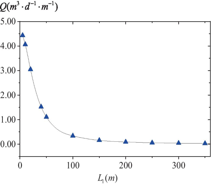
Relationship between groundwater inflow and distance between two adjacent circular drainage pipes
Based on the analysis above, the proposed analytical solution can generally be reduced to Goodman’s solution for an unlined tunnel. The difference between the proposed solution and Wang’s solution is less than 0.5% when the distance between two circular drainage pipes approaches infinitely small values. Therefore, both Goodman’s and Wang’s solutions can be considered specific cases of the proposed analytical solution.


Comparison to a numerical model
In this section, a three-dimensional numerical model is built using the FLAC3D. The numerical model consists of the surrounding rock, initial lining, circular drainage pipes, and geotextile (Fig. 7). The waterproof membranes and secondary lining serve as impermeable boundaries.

Numerical model
The dimensions of the numerical model are 100 × 100 m in length and width and 20 m in thickness. The parameters of the numerical model are presented in Table 1. For the boundary conditions, the top of the model is permeable with a constant hydrostatic head. The bottom, front, and back hydraulic boundaries are assumed to be impermeable. The left and right hydraulic boundaries are permeable and the corresponding water pressure is linear. The ground below the water level is fully saturated, whereas the water pressure in the drainage pipes is zero. The seepage path of groundwater flows from the surrounding rock into the initial lining, followed by the geotextile, reaches the circular drainage pipes. The groundwater is finally discharged through the drainage pipes. The numerical results and errors, as well as the results of the proposed analytical method adopting the same parameter values, are listed in Table 2.
Table 2 reveals that the groundwater inflows obtained using the numerical and proposed analytical solutions are in good agreement. The error between the two methods ranges from 1.9 to 7.3%.
Prediction of groundwater inflow using the WDSee model
The permeability coefficient of the rock (kr) surrounding a tunnel is a critical parameter for estimating groundwater inflow (Farhadian and Katibeh 2015). Therefore, kr was adopted as a reference index to analyze the effect of WDS on groundwater inflow. Figure 8 presents the results of groundwater inflow from Goodman’s solution (for an unlined tunnel), Wang’s solution (for a lined tunnel without considering the waterproof membranes, geotextiles, and circular drainage pipes of WDS), and the proposed analytical solution (for a lined tunnel considering all components of WDS).

Comparison of groundwater inflows between three analytical solutions
When kr is less than 1 × 10⁻⁸ m/s, the difference between the groundwater inflow obtained by Goodman’s solution and the other two solutions is less than 1%. This difference indicates that the tunnel lining has a small effect on groundwater inflow under this condition. Additionally, the maximum difference between Wang’s solution and the proposed analytical solution is only 0.6%. Therefore, the effects of WDS on groundwater inflow can be ignored. When kr ranges from 1 × 10⁻⁸ to 1 × 10⁻⁷ m/s, the differences among the three solutions remain insignificant. The difference between Wang’s solution and the proposed analytical solution increases to 5.7% at a permeability coefficient of 1 × 10⁻⁷ m/s, suggesting that the WDS effect on groundwater inflow can still be ignored. When kr is within the range of 1 × 10⁻⁷ to 1 × 10⁻⁶ m/s, the difference between Goodman’s solution and the other two solutions begins to increase and exceeds 43.9% at a permeability coefficient of 1 × 10⁻⁶ m/s, demonstrating that the effect of the lining on groundwater inflow is significant. The difference between Wang’s solution and the proposed analytical solution increases from 5.7 to 41.2%, demonstrating that the effects of WDS on groundwater inflow become more significant and cannot be ignored. Therefore, when kr exceeds 1 × 10⁻⁶ m/s, the WDS will significantly influence the amount of groundwater inflow and the effects of the WDS on groundwater inflow must be considered.
The percentage difference of the groundwater inflow between Wang’s solution and the proposed analytical solution (ξ=(Q − QWang) / Q×100%) was further analyzed to examine the effects of the WDS on groundwater inflow. Nine cases with varying permeability coefficients for the initial lining (k1) and outer radii of the initial lining (r2) were considered.
According to the results in Fig. 9, with an increase in kr, the difference in each case gradually increases to 10%. Furthermore, as k1 increases, the difference ξ becomes more significant and the maximum value exceeds 75%. This trend indicates that the effects of WDS on groundwater inflow are closely related to kr. Therefore, the influence of WDS is significant and cannot be ignored when kr exceeds 1 × 10⁻⁶ m/s.

The change on the percentage difference of groundwater inflow (ξ of Wang’s solution and the proposed analytical solution as a function of permeability coefficient of the surrounding rock
Parametric analysis
In this chapter, the relationships between groundwater inflow and each model parameter are analyzed. The parameters of the WDSee model include the water head, distance between two adjacent circular drainage pipes, thickness and permeability of the initial lining, and geotextile thickness and permeability, which are listed in Table 1. The results are presented in Figs. 10 and 11.

Relationships between groundwater inflow and model parameters; (a) water head, (b) distance between two adjacent circular drainage pipes, (c) thickness of initial lining, (d) geotextile hydraulic conductivity

Relationship between groundwater inflow and the permeability coefficient of the initial lining
Water head and rock permeability
As shown in Fig. 10a, the groundwater inflow increases with an increase in the water head and rock permeability, indicating that H and kr have a significant effect on groundwater inflow. For example, when kr is 8 × 10⁻⁸ m/s, the groundwater inflow increases nine times as h increases from 50 to 500 m. When H is 100 m, the groundwater inflow increases from 1.19 to 4.56 m3/d/m when kr increases from 8 × 10⁻⁸ to 5 × 10⁻⁷ m/s.
Distance between two adjacent circular drainage pipes
The relationship between the groundwater inflow and L1 is presented in Fig. 10b, indicating that the groundwater inflow gradually decreases with an increase in L1. When kr is greater than 3 × 10⁻⁷ m/s, the groundwater inflow decreases by approximately 50% as L1 increases from 4 to 20 m. When kr is less than 1 × 10⁻⁷ m/s, the groundwater inflow decreases by approximately 25% as L1 increases from 4 to 20 m. This trend indicates that L1 significantly influences groundwater inflow. Additionally, the higher the rock permeability, the more sensitive the groundwater inflow is to L1.
Thickness of the initial lining
The relationship between the groundwater inflow and thickness of the initial lining (T = r2 − r1) is presented in Fig. 10c, where the parameter r1 remains the same and the outer radius of the initial lining r2 increases from 5.7 to 6.05 m. It can be seen that the thickness of the initial lining has a weak effect on groundwater inflow. When kr is less than 1 × 10⁻⁷ m/s, the groundwater inflow remains approximately constant. When kr is greater than 3 × 10⁻⁷ m/s, the groundwater inflow decreases by approximately 14.5% as T increases from 0.1 to 0.45 m.
Geotextile hydraulic conductivity
The geotextile hydraulic conductivity (ktt) is the product of the geotextile permeability coefficient and geotextile thickness. The relationship between the geotextile hydraulic conductivity and groundwater inflow is presented in Fig. 10d. When ktt increases from 1 × 10⁻⁷ to 1 × 10⁻⁶ m2/s, the groundwater inflow increases by more than 45%. When ktt is greater than 1 × 10⁻⁶ m2/s, each curve in the figure tends to be flat. This trend indicates that ktt has a significant effect on groundwater inflow when it is within the range of 1 × 10⁻⁷ to 1 × 10⁻⁶ m2/s.
Permeability coefficient of the initial lining
The relationship between the permeability coefficient of the initial lining and groundwater inflow is presented in Fig. 11. When k1 increases from 1 × 10⁻⁹ to 1 × 10⁻⁸ m/s, the groundwater inflow gradually increases. Figure 11 reveals that k1 has an apparent effect on groundwater inflow under this condition. When k1 is greater than 1 × 10⁻⁸ m/s, each curve tends to be flat and the groundwater inflow increases by approximately 5%, indicating that k1 has a weak effect on groundwater inflow under this condition.
Suggestions on the WDS design
For a deeply buried tunnel subjected to a high water table (e.g., H > 150 m), the limitation of tunnel discharge rate less than 5.0 m3/d-m (Zhang et al. 2007; Zhang and Sun 2019) has been suggested to protect the ecological environment of the tunnel area. The WDS layout should be optimized to limit the discharge for an environmentally acceptable rate. Based on the parametric analysis, the groundwater inflow would exceed the discharge limitation when the permeability coefficient of surrounding rock kr is greater than 3 × 10⁻⁷ m/s, independent from the WDS layout parameters. Thus, in this condition, engineering techniques such as grouting might be needed to limit groundwater discharge. Conversely, discharge limitation can be met with proper WDS layout design when kr is less than 3 × 10⁻⁷ m/s. For example, limited discharge can be provided when the permeability coefficient of initial lining is less than 3 × 10⁻⁷ m/s, the distance between two adjacent circular drainage pipes is set to 10 m, and the geotextile hydraulic conductivity is less than 1 × 10⁻⁶ m2/s.
Discussion
The proposed analytical solution was motivated by considering the effects of WDS on the groundwater inflow for a deeply buried tunnel subjected to a high water table. The proposed analytical solution was derived based on the assumption (assumption (1)) that the tunnel cross-section is circular. While it is often not true in practical engineering, an equivalent circle shape may be used. In addition, the surrounding rock is assumed (assumption (2)) to be a continuous porous medium. In practice, the fractured rock mass is often considered as continuous media when the tunnel size is larger than the representative elementary volume (Li 2018). For example, rock mass can be assumed to be the continuous porous medium when small fissures are densely distributed (Wang et al. 2008). Therefore, the proposed analytical solution can also be applied to tunnels in fractured rock with densely distributed fractures. However, when the tunnel is shallow buried, or the rock mass cannot be considered as continuous media, the proposed analytical solution may not be suitable. Finally, the seepage path of groundwater is assumed (assumption (3)) to flow from the surrounding rock to the circular drainage pipes, which can be achieved when the lining type is the composite lining. Therefore, the proposed analytical solution is suitable for the composite lining with WDS.
Conclusions
In this study, the WDSee model was developed to consider all components of WDS. A corresponding analytical solution for groundwater inflow into a composite lining tunnel was derived. WDS components were fully considered when deriving the proposed analytical solution, which was then validated using a numerical model. A parametric study was conducted to investigate the relationships between groundwater inflow, and geometric and physical parameters. The following conclusions can be drawn.
-
1.
The proposed analytical solution is useful for estimating groundwater inflow into a tunnel with a composite lining. Such analytical solutions can be applied to deeply buried rock tunnels that are subjected to a high water table. The proposed analytical solutions can be reduced to Goodman’s solution for unlined tunnels. The difference between the proposed analytical solution and an existing solution (e.g., Wang’s solution) is less than 0.5% for an infinitesimal distance between two adjacent circular drainage pipes.
-
2.
The effects of WDS on groundwater inflow are influenced by rock permeability. The higher the rock permeability coefficient, the more significant the effect. When the rock permeability coefficient of the surrounding rock exceeds 1 × 10⁻⁶ m/s, the effects of WDS cannot be ignored.
-
3.
The groundwater inflow into a tunnel is closely related to the geometric and physical parameters of the tunnel. Geometric parameters include the initial lining thickness, radius of the affected zone by the drainage, distance between adjacent circular drainage pipes, and geotextile thickness. Physical parameters include the water head and permeability coefficients of the initial lining, surrounding rock, and geotextile. The groundwater inflow significantly decreases with an increase in the distance between adjacent circular drainage pipes. Furthermore, the higher the rock permeability coefficient, the more significant the effect of the geometric and physical parameters of the tunnel.
-
4.
When the permeability coefficient of the surrounding rock kr is greater than 3 × 10⁻⁷ m/s, engineering techniques such as grouting might be needed to limit groundwater discharge under high water table (e.g., H > 150 m) to meet environment protection needs. Conversely, discharge limitation can be met with proper WDS layout design when kr is less than 3 × 10⁻⁷ m/s.
Abbreviations
- r 0 :
-
Inner radius of the secondary lining (m)
- r 1 :
-
Outer radius of the secondary lining (m)
- r 2 :
-
The outer radius of the initial lining (m)
- r 3 :
-
Radius of the affected zone by the drainage
- h 2 :
-
Water head around the outside of the initial lining (m)
- h c :
-
Water head at the geotextile (m)
- H :
-
Water head outside of the affected drainage zone in the surrounding rock (m)
- h m :
-
Water head in the middle of the two adjacent circular drainage pipes (m)
- q :
-
Velocity of groundwater flowing into the circular drainage pipe from the geotextile
- k 1 :
-
Permeability coefficients of the initial lining (m)
- k r :
-
Permeability coefficients of surrounding rock (m/s)
- L 1 :
-
Distance between the two adjacent circular frainage pipes (m)
- k t :
-
Permeability coefficients of the geotextile (m/s)
- t :
-
Geotextile thickness (m)
- T :
-
Thickness of initial lining, r2-r1 (m)
- D :
-
Diameter of the circular frainage pipe (m)
- μ :
-
The drain coefficient
- Q :
-
Groundwater inflow into the tunnel (m3/d m)
References
Arjnoi P, Jeong JH, Kim CY, Park KH (2009) Effect of drainage conditions on porewater pressure distributions and lining stresses in drained tunnels. Tunn Undergr Space Technol 24(4):376–389
Bear J (1972) Dynamics of Fluids in Porous Media. American Elsevier Publishing Company, New York
Bobet A (2016) Deep tunnel in transversely anisotropic rock with groundwater flow. Rock Mech Rock Eng 49(12):4817–4832
Butscher C (2012) Steady-state groundwater inflow into a circular tunnel. Tunn Undergr Space Technol 32:158–167. https://doi.org/10.1016/j.tust.2012.06.007
Cheng P, Zhao LH, Luo ZB et al (2019a) Analytical solution for the limiting drainage of a mountain tunnel based on area-well theory. Tunn Undergr Space Technol 84:22–30. https://doi.org/10.1016/j.tust.2018.10.014
Cheng P, Zhao LH, Li Q, Li L, Zhang S (2019b) Water inflow prediction and grouting design for tunnel considering nonlinear hydraulic conductivity. KSCE J Civ Eng 23(9):1–9
Ding H, Jiang SP, Li Y (2007) Study on waterproof and drainage techniques of tunnels based on controlling drainage. J Geotech Eng 29(9):1398–1403
Du CW, Wamg MS, Tan ZS (2011) Analytic solution for seepage filed of subsea tunnel and its application. J Rock Mech Eng 30(S2):3567–3573
El-Tani M (2003) Circular tunnel in a semi-infinite aquifer. Tunn Undergr Space Technol 18:49–55
Farhadian H, Katibeh H (2015) Groundwater seepage estimation into Amirkabir tunnel using analytical methods and DEM and SGR method. Int J Civil Environ Eng 9(3):296–301
Farhadian H, Katibeh H (2017) New empirical model to evaluate groundwater flow into circular tunnel using multiple regression analysis. Int J Min Sci Technol 27(3):415–421. https://doi.org/10.1016/j.ijmst.2017.03.005
Farhadian H, Katibeh H, Huggenberger P, Butscher C (2016) Optimum model extent for numerical simulation of tunnel inflow in fractured rock. Tunn Undergr Space Technol 60:21–29. https://doi.org/10.1016/j.tust.2016.07.014
Farhadian H, Nikvar Hassani A, Katibeh H (2017) Groundwater inflow assessment to Karaj Water Conveyance tunnel, northern Iran. KSCE J Civ Eng 21(6):2429–2438
Farhadian H, Nikvar-Hassani A (2018) Water flow into tunnels in discontinuous rock: a short critical review of the analytical solution of the art. Bull Eng Geol Env 78(5):3833–3849. https://doi.org/10.1007/s10064-018-1348-9
Gokdemir C, Rubin Y, Li XJ, Li YD, Xu H (2019) Vulnerability analysis method of vegetation due to groundwater table drawdown induced by tunnel drainage. Adv Water Resour 133:103406–103418. https://doi.org/10.1016/j.advwatres.2019.103406
Gokdemir C, Yoram Rubin Y, Li XJ, Xu H (2021) A vulnerability assessment method to evaluate the impact of tunnel drainage on terrestrial vegetation under various atmospheric and climatic conditions. Adv Water Resour 147:103796–103811. https://doi.org/10.1016/j.advwatres.2020.103796
Goodman R, Moye D, Schalkwyk A, Javendel I (1965) Groundwater inflow during tunnel driving. Eng Geol 1:150–162
Harr ME (1962) Groundwater and Seepage. McGrawHill, New York
Hassani NA, Farhadianb H, Katibeh H (2018) A comparative study on evaluation of steady-state groundwater inflow into a circular shallow tunnel. Tunn Undergr Space Technol 73:15–25
He BG, Zhang ZQ, Fu SJ, Liu YJ (2015) An analytical solution of water loading on tunnel supporting system with drainage of blind tube and isolation effect of waterproof membranes. J Rock Mech Eng 34:3936–3947
Heuer RE (2005) Estimating rock tunnel inflow. Rapid Excavation Tunn Conf 30:394–407
Huang FM, Wang MS, Tan ZS, Wang XY (2010) Analytical solutions for steady seepage into an underwater circular tunnel. Tunn Undergr Space Technol 25:391–396
Katibeh H, Aalianvari A (2009) Development of a new method for tunnel site rating from groundwater hazard point of view. J Appl Sci 9(8):1496–1502
Kolymbas D, Wagner P (2007) Groundwater ingress to tunnels – The exact analytical solution. Tunn Undergr Space Technol 22(1):23–27
Li G, Ma W, Tian S, Zhou H (2021) Zou W (2021) Groundwater inrush control and parameters optimization of curtain grouting reinforcement for the jingzhai tunnel. Geofluids 7:1–10
Li XJ, Li YD, Chang CF, Tan B, Chen ZY, Sege J, Wang C, Rubin Y (2018a) Stochastic goal-oriented rapid impact modeling of uncertainty and environmental impacts in poorly-sampled sites using ex-situ priors. Adv Water Resour 111:174–191
Li P, Wang F, Long Y, Xu Z (2018b) Investigation of steady water inflow into a subsea grouted tunnel. Tunn Undergr Space Technol 80:92–102
Li W (2018) Characteristic scales for permeable property of fractured rock masses in typical flow configurations and engineering applications. Dissertation, Shandong University
Liu K (2017) Study on external water pressure and force characteristics of tunnel lining with partial blocked drainage system. Dissertation, Chongqing University
Maleki RM (2018) Groundwater Seepage Rate (GSR): a new method for prediction of groundwater inflow into jointed rock tunnels. Tunn Undergr Space Technol 71:505–517
Mikaeil R, Doulati Ardejani F (2009) Prediction of groundwater inflow into tunnels using numerical models; a practical case study: Kuhin railway tunnel, Qazvin-Rasht. Iran Int J Eng Sc 19(9):65–73
Ministry of Railways of the People's Republic of China (2004) Code for hydrogeological investigation of railway engineering. TB 10049–2004. China Railway Press, Beijing
Murillo CA, Shin JH, Kim KH, Colmenares JE (2014) Performance tests of geotextile permeability for tunnel drainage systems. KSCE J Civ Eng 18(3):827–830
Nikvar-Hassani A, Katibeh H, Farhadian H (2016) Numerical analysis of steady-state groundwater inflow into Tabriz line 2 metro tunnel, northwestern Iran, with special consideration of model dimensions. Bull Eng Geol Env 75(4):1617–1627
Oshima (1983) Railway Technology Research Report. Railway Technical Research Institute, Tokyo
Park KH, Owatsiriwong A, Lee JG (2008) Analytical solution for steady-state groundwater inflow into a drained circular tunnel in a semi-infinite aquifer: a revisit. Tunn Undergr Space Technol 23:206–209
Park YJ, Hwang HT, Suzuki S, Saegusa H, Nojiri K, Tanaka T, Bruines P, Abumi K, Morita Y, Illman WA (2020) Improving precision in regional scale numerical simulations of groundwater flow into underground openings. Eng Geol 274:1–8. https://doi.org/10.1016/j.enggeo.2020.105727
Sedghi MM, Samani N (2015) Semi-analytical solutions for flow to a well in an unconfined-fractured aquifer system. Adv Water Resour 83:89–101
Su K, Zhou YF, Wu HG, Shi CZ, Zhou L (2017) An analytical method for groundwater inflow into a drained circular tunnel. Ground Water 55(5):712–721
Sweetenham MG, Maxwell RM, Santi PM (2017) Assessing the timing and magnitude of precipitation-induced seepage into tunnels bored through fractured rock. Tunn Undergr Space Technol 65:62–75. https://doi.org/10.1016/j.tust.2017.02.003
Tan Y, Smith JV, Li CQ, Currell M, Wu YF (2018) Predicting external water pressure and cracking of a tunnel lining by measuring water inflow rate. Tunn Undergr Space Technol 71:115–125. https://doi.org/10.1016/j.tust.2017.08.015
Tang Y, Chan DH, Zhu DZ (2018) Analytical solution for steady-state groundwater inflow into a circular tunnel in anisotropic soils. J Eng Mech 144(9):1–8
Wang JY (2003) Once more on hydraulic pressure upon lining. Mod Tunn Technol 40(3):5–9
Wang XY, Tan ZS, Wang MS, Zhang M, Huang FM (2008) Theoretical and experimental study of external water pressure on tunnel lining in controlled drainage under high water level. Tunn Undergr Space Technol 23(5):552–560
Wang XY, Wang MS, Zhang M (2004) A simple method to calculate tunnel discharge and external water pressure on lining. J Northern Jiaotong University 28(1):8–10
Wang YC (2006) Tunnel Engineering. China Communications Press, Beijing
Wei ZL, Wang DF, Xu HD, Sun HY (2020) Clarifying the effectiveness of drainage tunnels in landslide controls based on high-frequency in-site monitoring. Bull Eng Geol Env 79(7):3289–3305
Wu JC, Xue YQ (2006) Groundwater dynamics. China Water Power Press, Beijng
Xiao CL, Liang XJ, Wang B (2009) Hydrogeology. Tsinghua University Press, Beijng
Xie HS, Jiang C, He JL, Han HX (2019) Analytical solution for the steady-state karst water inflow into a tunnel. Geofluids 2019:1–9. https://doi.org/10.1155/2019/1756856
Yang G, Wang X, Wang X, Cao Y (2014) Analyses of seepage problems in a subsea tunnel considering effects of grouting and lining structure. Mar Georesour Geotechnol 34(1):65–70. https://doi.org/10.1080/1064119X.2014.958882
Ying HW, Zhu CW, Shen HW, Gong XN (2018) Semi-analytical solution for groundwater ingress into lined tunnel. Tunn Undergr Space Technol 76:43–47. https://doi.org/10.1016/j.tust.2018.03.009
Zarei HR, Uromeihy A, Sharifzadeh M (2013) A new tunnel inflow classification (TIC) system through sedimentary rock masses. Tunn Undergr Space Technol 34:1–12
Zhang CP, Zhang DL, Wang MS, Xiang YY (2007) Study on the appropriate parameters of grouting cycle for tunnels with limiting discharge lining in high water pressure and water-enriched region. J Rock Mech Eng 26(11):2270–2276
Zhang DL, Sun ZY (2019) An active control waterproof and drainage system of subsea tunnels and its design method. J Mech Eng 38(1):1–17
Zhang W, Dai B, Liu Z, Zhou C (2017) On the non-Darcian seepage flow field around a deeply buried tunnel after excavation. Bull Eng Geol Env 1:1–14. https://doi.org/10.1007/s10064-017-1041-4
Zhang ZD (2006) Semi-theoretical derivation for the solutions of water inflow and water pressure acting on a tunnel and their application to the waterproofing and drainage of tunnels. Mod Tunn Technol 43(1):1–7
Zhao L, Ting R, Wang NB (2017) Groundwater impact of open cut coal mine and an assessment methodology: A case study in NSW. Int J Min Sci Technol 27:861–866. https://doi.org/10.1016/j.ijmst.2017.07.008
Funding
This study was supported by the National Natural Science Foundation of China (Grant No. 41877246), Department of Transport of Yunnan Province (Grant No. [2019]36). The authors greatly appreciate the support provided.
Author information
Authors and Affiliations
Corresponding author
Additional information
Highlights
• An analytical solution for estimating groundwater inflow into lined tunnel considering waterproofing and drainage system (WDS) is proposed.
• The components of the waterproofing and drainage systems (waterproof membranes, geotextile, and blind pipes) could be consider.
• The proposed analytical solution is applied to analyze the WDS effect on the groundwater inflow into the tunnel.
Rights and permissions
About this article

Cite this article
Liu, J., Li, X. Analytical solution for estimating groundwater inflow into lined tunnels considering waterproofing and drainage systems. Bull Eng Geol Environ 80, 6827–6839 (2021). https://doi.org/10.1007/s10064-021-02378-0
Received:
Accepted:
Published:
Issue Date:
DOI: https://doi.org/10.1007/s10064-021-02378-0