
Abstract
A novel method for daily temperature and precipitation downscaling is proposed in this study which combines the Ensemble Optimal Interpolation (EnOI) and bias correction techniques. For downscaling temperature, the day to day seasonal cycle of high resolution temperature of the NCEP climate forecast system reanalysis (CFSR) is used as background state. An enlarged ensemble of daily temperature anomaly relative to this seasonal cycle and information from global climate models (GCMs) are used to construct a gain matrix for each calendar day. Consequently, the relationship between large and local-scale processes represented by the gain matrix will change accordingly. The gain matrix contains information of realistic spatial correlation of temperature between different CFSR grid points, between CFSR grid points and GCM grid points, and between different GCM grid points. Therefore, this downscaling method keeps spatial consistency and reflects the interaction between local geographic and atmospheric conditions. Maximum and minimum temperatures are downscaled using the same method. For precipitation, because of the non-Gaussianity issue, a logarithmic transformation is used to daily total precipitation prior to conducting downscaling. Cross validation and independent data validation are used to evaluate this algorithm. Finally, data from a 29-member ensemble of phase 5 of the Coupled Model Intercomparison Project (CMIP5) GCMs are downscaled to CFSR grid points in Ontario for the period from 1981 to 2100. The results show that this method is capable of generating high resolution details without changing large scale characteristics. It results in much lower absolute errors in local scale details at most grid points than simple spatial downscaling methods. Biases in the downscaled data inherited from GCMs are corrected with a linear method for temperatures and distribution mapping for precipitation. The downscaled ensemble projects significant warming with amplitudes of 3.9 and 6.5 °C for 2050s and 2080s relative to 1990s in Ontario, respectively; Cooling degree days and hot days will significantly increase over southern Ontario and heating degree days and cold days will significantly decrease in northern Ontario. Annual total precipitation will increase over Ontario and heavy precipitation events will increase as well. These results are consistent with conclusions in many other studies in the literature.
1 Introduction
Global mean surface temperature changes for the period till the end of the twenty-first century are projected to likely exceed 1.5 °C relative to the 1850–1900 (IPCC, Field et al. 2014). In south-central Canada, extreme temperature related weather presents a much greater risk to human health during heat waves (Cheng et al. 2008a). As temperature increases, heat-related mortality is projected to be more than doubled by 2050s and tripled by 2080s from the current condition (Cheng et al. 2008b). As the most populated and the second largest province of Canada, Ontario is vulnerable to climate change (Chiotti and Lavender 2008). Over Ontario, there is no significant trend in annual precipitation for the period 1951–2010, except for the southern area where exists a significant increasing trend (Mach and Mastrandrea 2014). The annual heavy precipitation days, very heavy precipitation days and very wet days and extreme wet days are projected to significantly increase over major parts of Ontario under the A2 scenario (Deng et al. 2016). The 5th assessment report (AR5) of the IPCC (2014) concludes that Global warming leads to an intensification of the water cycle and attendant effects on heavy and extreme precipitation events and is likely to lead to more frequent daily precipitation extremes. These changes are important for a number of potential impacts, including floods, erosion, water resources, agriculture and ecosystems (IPCC, Field et al. 2014). Thus, it becomes increasingly important for the provincial and municipal governments as well as the public to be aware of future climate changes at local scales. High resolution climate projection data at multiple time scales (annual, monthly and daily) is necessary for governments to develop climate adaptation/mitigation strategies to address local impacts.
The geography of Ontario is significantly different from other areas in Canada. It is bordered by Great Lakes, Hudson Bay and James Bay. Within Ontario, there are more than 250,000 small lakes, large areas of uplands, particularly within the Canadian Shield which traverses the province from northwest to southeast and also above the Niagara Escarpment in the south. Southern Ontario (south of Lake Nipissing) belongs to Great Lakes/St. Lawrence River Basins (Environment Canada 1998; Chadwick and Hume 2009). To generate projections of climate change in Ontario, impacts of all these specific geography features should be considered (Szeto 2008). The IPCC CMIP5 GCMs could not provide a suitable description of the orographic effects and land-surface characteristics due to their lower spatial resolution. There are several methods that can be used to generate region-specific climate information, for example high-resolution atmospheric GCMs (AGCMs), variable-resolution global models, and statistical and dynamical downscaling (Flato et al. 2013). Among these methods, the most widely used are the dynamical and statistical downscaling. To better represent the sub-grid-scale meteorological characteristics, Regional Climate Models (RCM) offer an elegant way to integrate local processes through physical and dynamical equations. However, they can be extremely computer-intensive (Schoof 2015). It is impossible to produce a large ensemble of decades-long simulations for multiple GCMs and/or emissions scenarios (Maurer and Hidalgo 2007). Statistical downscaling uses statistical equations to convert global-scale output to regional-scale conditions. It needs much less computational effort than dynamical downscaling. Thus, it offers the opportunity to use “ensemble” GCM results and are widely used in regional climate change studies. Statistical downscaling assumes that there is a strong relationship between the predictor and predictand and the relationships between large and local-scale processes will remain the same in the future (stationarity assumptions). There are several categories of statistical downscaling techniques, such as linear methods, weather classification, weather generator, etc. A unique class of downscaling techniques where the predictor and predicted variables are the same, albeit of different scale, have been widely used to produce large ensemble for different GCMs and/or multiple emission scenarios. An extensively used method of this class is the bias corrected spatial disaggregation (BCSD) statistical downscaling approach and its modified versions (Wood et al. 2002, 2004; Maurer and Hidalgo 2007; Werner 2011; Gutmann et al. 2014; Rana and Moradkhani 2015; Ning et al. 2015). In this method, averages of temperature and precipitation are used to develop empirical statistical relationships between large-scale and local-scale variables (Werner 2011). The local intensity scaling (LOCI, Schmidli et al. 2006) method is another example of this class of techniques (Schmidli et al. 2007; Gao et al. 2014; Deng et al. 2016). It is a direct downscaling and error correction method (DECM). The basic idea of this method is that climate model output integrates all relevant predictors. Deviations between climate model output and regional- or local-scale observations are in first order due to systematic climate model errors and an incomplete or inaccurate representation of the orography (Schmidli et al. 2007). A necessary step of the above mentioned direct downscaling methods is to interpolate GCM data onto target grid points or stations using spatial interpolation considering the effects of a few geographic factors (e.g., distance, elevation, slope, etc). These factors are generally stationary in time. Simple statistical downscaling methods are usually unable to keep spatial and temporal consistency, or inter-variable consistency and therefore suffer from possible out-of-sample issues (Benestad 2005).
In this study, we propose a novel downscaling method motivated by the idea of data assimilation (Kalnay 2003). In data assimilation, both observations and numerical models are treated as sources of information and the most likely state of the atmosphere is estimated from a set of observations and an atmospheric circulation model. Instead of assimilating observations, the proposed downscaling methods ‘assimilates’ output of GCM into a statistical model whose climatology and covariance matrix are extracted from the high resolution NCEP climate forecast system reanalysis (CFSR, Saha et al. 2010, 2013). EnOI framework proposed by Evensen (2003), which is widely used in data assimilation practice (Oke et al. 2005; Deng et al. 2011, 2012; Sakov and Sandery 2015; Qi and Cao 2015; Srinivasan et al. 2011), will be employed in this study. The transfer function of the EnOI is constructed using the output of NCEP climate forecast system (CFS) which keeps spatial and temporal consistency. Therefore, this method can better represent influencies of local geographic factors on local climate than traditional interpolation methods. Using this method, daily temperatures (mean, maximum and minimum) and precipitation from 29 members of IPCC AR5 RCP 8.5 GCMs are transferred to the high resolution grid points (0.3125° × 0.3125°) of CFSR and biases are further corrected. Temperatures are corrected with a linear rescaling method and precipitation is corrected with Gamma distribution mapping.
The rest of the paper is organized as the following. Section 2 describes the data sets used in this study. Section 3 provides details of the EnOI downscaling method, its validation and the methods for bias correction. In Sect. 4 we present the downscaled temperatures and precipitation over Ontario from an ensemble of GCMs under the IPCC RCP8.5 (representative concentration pathway 8.5) scenario. Finally, we end the paper in Sect. 5 with conclusions and a brief discussion.
2 Data
2.1 Observations
Observations from 1981 to 2010 at 54 Ontario weather stations are downloaded from the Environment and Climate Change Canada (ECCC) website (http://climate.weather.gc.ca/climate_normals/index_e.html). These 54 stations (Fig. 1a) meet the WMO “3 and 5 rule” (i.e. no more than 3 consecutive and no more than 5 total missing for either temperature or precipitation) (Braun et al. 2015). Variables/indices downloaded include averages of the temperatures, Cooling Degree Days (CDD, Tm > 18 °C) and Heating Degree Days (HDD, with Tm < 18 °C), Days with Tx above 30 °C (DTX30) and Days with Tn below − 20 °C (DTN20), total precipitation, extreme daily precipitation, days with precipitation ≥ 5, 10 and 25 mm. The definition of these indices can be found in Environment Canada (2012). Averages of these climate variables will be used for downscaling model evaluation and validation.

Map of the studied region (Ontario,Canada). (Left) locations of CCSM4 grid points within the 350 km buffer region (Buffer_On), 1522 CFSR grid points within Ontario (solid black dot), 54 weather stations (red cross) and a selected CFSR grid point (red dot). (Right) the topography of Ontario
2.2 Reanalysis data
Reliable daily observation data at high spatial resolution is the key to developing statistical downscaling models for daily variables. However, as shown in Fig. 1a, most of the stations are located in southern Ontario and there is no observation over the majority of the central and northern Ontario. Alternatively, reanalysis products represent spatially complete and dynamically-consistent estimates of the state of the climate system (Dee at al. 2011). There are several high resolution (< 50 km) daily reanalysis datasets that cover the entire province, for example the new generation of ECMWF reanalysis climate data (ERA-interim, Dee et al. 2015), the NCEP North America Regional Reanalysis (NARR, Mesinger et al. 2004) and the NCEP climate forecast system reanalysis (CFSR, Saha et al. 2010, 2013). In this study, daily mean, minimum and maximum near surface temperatures and precipitation (Tm, Tn, Tx and Pr respectively) from the CFSR over the region between 101°W–70°W longitude and 38°N–60°N latitude for the period from January 1, 1981 to December 31, 2010 are used for constructing the downscaling models. The CFSR is a third generation global reanalysis product, with higher temporal (6-h) and spatial resolution (0.313° × ~ 0.312°) completed at the NCEP. The NCEP CFS is a global, high-resolution, coupled atmosphere-ocean-land and surface-sea-ice system to provide the best estimate of the state of earth system, it can resolve fine scale weather and land-surface processes in response to the large-scale forcing. It has assimilated observations from many data sources (Saha et al. 2010, 2013; Wang et al. 2011). Especially, CFSR assimilated many hydrological quantities from a parallel land surface model forced by the NOAA’s Climate Prediction Center (CPC) pentad merged analysis of precipitation and the CPC unified daily gauge analysis (Wang et al. 2011). Thus, it could better represent the effects of land surface process on precipitation. CFSR data is chosen in this study for downscaling model construction and cross-validation due to its good quality and high resolution that meet the requirements of this study. For validation of the downscaling model, the four variables from the NCEP-DOE Reanalysis 2 data (1.875° lon × 1.91° lat) provided by the NOAA/OAR/ESRL PSD, Boulder, Colorado, USA, from their Web site at http://www.esrl.noaa.gov/psd/ are also used in this study.
2.3 GCM data
Daily data (Tm, Tn, Tx and Pr) from 29 GCMs of CMIP5 under the scenario RCP8.5 (Table 1) are extracted from the Earth System Grid (ESG) data portal (http://cera-www.dkrz.de/WDCC/ui/). Though most models have multiple ensemble members, without knowledge about which member is better than other members over Ontario, only the first member from each model is used. Thus, each model used in this study is given equal weight when perform simple model statistical analysis on the downscaled ensemble (Moss et al. 2010; Flato et al. 2013). Any knowledge about the performance of the model is neglected (Casanova and Ahrens 2009). Only several models have historical simulations after 2005 (i.e. 2006–2012); therefore, in this study we consider 1981–2005 to be the reference period for bias correction. Changes over two 30-year periods, 2050s (2041–2070, the mid-century) and 2080s (2071–2100, the end of-century) relative to present, 1990s (1981–2010), are investigated. Accordingly, results from temperatures, precipitation and some derived variables are analysed and presented for these three time periods. Only data in a buffer region which wraps Ontario are used for downscaling (Fig. 1a). GIS software ArcGIS 10.1 (Law and Collins 2013; Pimpler 2013; Armstrong 2015) was used to create a 350 km buffer for each of the CFSR grid points within Ontario and then merge all of the individual buffer zones to obtain the integrated buffer region for the province. The reason why the value 350 km is selected will be described in Sect. 3.
3 Downscaling methods
The proposed downscaling method includes three steps. First, GCM data is transferred to the CFSR grid points within Ontario using the EnOI method; then, the biases are removed by a linear scaling method for temperatures and monthly total precipitation amount; and finally the variance amplitudes of temperatures and monthly precipitation are adjusted using a variance scaling method. For daily precipitation, only wet day (pr > = 1.0 mm) precipitation is corrected with Gamma distribution fitting. Details of these steps will be presented in the following subsections.
3.1 Transfer GCM temperatures to CFSR grid points
Data assimilation incorporates observations into the model state of a numerical model by taking the weighted mean of the observations and the model state. The resulting analysis is considered to be the ‘best’ estimate of the state of the atmosphere (ocean or other systems) at a particular time. EnOI is a computationally efficient data assimilation method (Evensen 2003; Oke et al. 2005), which will be used in this study to downscale GCM projections to CFSR grid points within Ontario. Typical EnOI analysis is computed by solving the following equation (Oke et al. 2005; Deng et al. 2011, 2012; Sakov and Sandery 2015; Qi and Cao 2015; Srinivasan et al. 2011):
where \(X\) is the state vector;gain matrix (\(K\)) is:
\(P\) is model error covariance matrix estimated from model error\({X^{\prime} }\)
R is observation error covariance matrix estimated from observation error \(\Upsilon\) and it is a diagonal matrix because the observation error is assumed to be uncorrelated in space and time:
\(H\) is an operator that interpolates from model grid to observation locations; \(HX\) is the interpolated model data at observation locations; \(~Y\) is observations; \(\left( {Y - HX} \right)\) is the difference between observation and model; α is a scalar that can be used to tune the magnitude of the covariance for a particular application; C is a correlation matrix for localization in the horizontal around each observation, its elements are generally defined by the quasi-Gaussian function in Gaspari and Cohn (1999); superscript a, T, −1 and \(\prime\) denote respectively analysis, matrix transposition, inverse and error; The open circle between C and P denotes a Schur product (an element by element matrix multiplication). For details please refer to (Evensen 2003; Oke et al. 2005; Deng et al. 2010, 2011, 2012; Sakov and Sandery 2015; Qi and Cao 2015; Srinivasan et al. 2011). Analyses in this study followed the following 6-step approach (a–f).
-
(a)
We assume the 365-day annual cycle in the CFSR data as a state model and the GCM output as observations. Under such assumption, we can use Eq. (1) to downscale GCM temperatures to CFSR grid points. Differing from true dynamical model, the seasonal cycle model does not include the interannual variation which will alternatively be incorporated into the algorithm by assimilating GCM output through Eq. (1). Based on CFSR daily data from 1981 to 2010, we estimate the gain matrix(K) using the following steps.
-
(b)
For simplicity, in the Eq. (2) the parameter α is set to 1 and each element of C is set to a step function. When generating the values at a CFSR grid point using Eq. (1), it is reasonable to only consider data at L GCM grid points (defined below) close to the analysis CFSR grid point and ignore other distant GCM grid points. If a GCM grid point is one of the L grid points we denote it as a type-A GCM grid point, otherwise as a type-B GCM grid point. Then the element of localization matrix C is:
$$c=\left\{ {\begin{array}{*{20}{c}} {1,~}&{type - A~GCM~grid~point} \\ {0,~}&{type - B~GCM~grid~point} \end{array}} \right..$$(5)The parameter L is model dependent and is a function of model horizontal resolution and decorrelation distance (DD) of the variable to be downscaled. DD is defined by World Meteorological Organization (WMO) as the distance where the square of spatial autocorrelation decrease to below 0.5 (Carrega 2013; Jarraud 2008). In this study, the 30-year CFSR daily temperature is used to estimate the DD. Seasonal cycle was removed before calculating the autocorrelation coefficients (CORR) between different grid points. Figure 2a–c show the relationship between CORR and distances for daily mean temperature (Tm), maximum temperature (Tx) and minimum temperature (Tn), respectively. It is observed that the CORR decrease with the increase of distance. Averaged over the province, the value of DD is 606 (504 ~ 695) kilometers (km), 514 (357 ~ 628) km and 494 (346 ~ 590) km for Tm, Tx and Tn (see the cross points), respectively. The smaller DD values for extreme temperatures are due to the fact that extreme events are more sensitive to local geographical conditions; and for the same reason, DD varies in space as well. Figure 2d–f show the spatial distributions of DD for Tm, Tx and Tn. It is observed that DDs are similar in spatial distribution pattern among the 3 variables. For example, the values of DD are larger in the northern area than in the southern area with maximum value in the region west of 94°W and minimum value in the southwestern Ontario. This DD spatial pattern corresponds to the topography shown in Fig. 1b. Differences in amplitude of the values among the 3 variables are obvious. Probably the ideal situation is to use the spatial varying DD as threshold for searching type-A GCM grid points (defined in Eq. 5) for each of the CFSR grid points. However, the spatial varying DD may lead to problems such as the downscaled variable being too smooth when DD is large, and this algorithm becomes over complicated and much less computational effective. For simplicity, we select 350 km as the threshold for GCM model grid point searching because it is close to the minimum value of DD in Ontario. After this threshold is determined, the type-A grid points at each of the CFSR grid points for each model will be automatically selected by a searching algorithm or by GIS software ArcGIS (Pimpler 2013; Law and Collins 2013). The number of type-A grid points varies with locations of the CFSR and GCM grid points. There are at least four Type-A GCM grid points at each of CFSR grid points for all GCMs except for CMCC-CESM which has a very low resolution (3.75° in longitude and latitude). To make point search more effective, we search four nearest grid points for this special model instead of using the above discussed searching algorithm. Therefore, there will be four type-A grid points at CFSR grid points for the CMCC-CESM (with the coarsest resolution) whereas more than 100 type-A grid points at high latitude for model CMCC-CM (with the finest resolution, 0.75° in longitude and latitude).
Fig. 2 
Variation of spatial autocorrelation coefficient as function of distance (upper panel) and the spatial distribution of decorrelation distances (\({r}^{2}\) decreasing below 0.5). The cross point in (a–c) is the mean decorrelation distances averaged over Ontario. The black points represent the relation for individual grid points in Ontario
-
(c)
Since we use a 365-day climatology of CFSR data as the state model, the anomaly relative to the climatology is the error of the model and the error covariance matrix \(({X^\prime }{X^{\prime T}})\) in Eq. (3) equals to the anomaly covariance matrix. For downscaling daily temperature, we construct the error covariance matrices using an enlarged ensemble to consider the larger range of weather condition for each calendar day. All anomalies within a 15-day window are considered as the anomalies on the day at the center of the window. For example, the window for May 20 and December 3 is [May 13–May 27] and [November 26–December 10], respectively. Therefore, the ensemble size is enlarged from 30 to 450. The daily climate mean is also estimated with this 450-member ensemble. This large ensemble can reflect various possible weather situations around the calendar day in the climate system represented by the day to day climate cycle. Since CFSR data is the output from CFS which has resolved fine-scale weather and land-surface processes in respond to the large-scale forcing, the covariance matrixes of CFS at daily time scale could represent the spatial correlation structure between different grid points caused by the small scale (i.e., at CFSR grid resolution) geographical factors (e.g., elevations, landscape, land cover etc.). If output from a regional climate model (RCM) is used to construct the downscaling model, the procedure is the same.
-
(d)
We use the inverse distance weighting (IDW) method to construct the linear operator H. Since the resolution of CFSR data (~ 0.3125°) is much higher than that of GCMs, interpolate the high resolution data to low resolution GCM grid point is easy. At first, search for the four nearest CFSR grid points around each GCM grid point, calculate the distances (< ~ 35 km in Ontario) between that GCM grid point and the four nearby CFSR grid points, and establish the normalized inverse of the distances as the weight for IDW. Thus, H is a sparse matrix with a dimension of \(N \times 1552\), where \(N\) (see Table 1) is the total number of GCM grid points from which data would be considered for the downscaling and 1552 is the total number of the CFSR grid points within Ontario. The values of \(N\) depend on the GCM grid system, for example the minimum value of N is 30 for CMCC and the maximum value of N is 725 for CMCC-CM. With the estimated operator H, it is straightforward to calculate the term HX. The term \(\alpha \left( {{\mathbf{C}} \circ \left( {{X^\prime }{X^{\prime T}}} \right)} \right){H^T}\) is the localized covariance matrix between CFSR grid points and GCM grid points \(\left( {a~1552 \times N~matrix} \right)\) and the term \(\alpha H\left( {{\mathbf{C}} \circ \left( {{X^\prime }{X^{\prime T}}} \right)} \right){H^T}\) is the localized covariance matrix of GCM grid points \(\left( {an~N \times N~matrix} \right)\). Therefore, Eq. (1) has considered the relationships between different CFSR grid points, between CFSR grid points and GCM grid points and between different GCM grid points. These relationships reflect the comprehensive impacts of geographic conditions on weather and climate.
-
(e)
In a real data assimilation system, R is the errors in observations. In present paper, the goal of the first step (a) is to transform the information from GCMto CFSR grid points by the gain matrix. A large R may force the system towards CFSR seasonal cycle and loss the signal of future climate change in the output of the GCMs. So, in this study we set R as a small fraction (10%) of the diagonal of the model error covariance matrix P. Thus, the downscaled data will be dominated by the information transferred by the gain matrix from GCMs. This is the goal of all downscaling practice. The treatment is reasonable because generally at the location where the anomaly is large the GCMs may have a large error as well. The negative impacts of the arbitrary small constant will be reduced in bias correction steps. We tried other small values (e.g., 0.5, 1 and 5%), their impacts to the final result are negligible. This error estimation method is widely used when it is difficult to estimate the errors in observations (Deng et al. 2012; Hopson 2014). The problem caused by the small error assumption is similar to that in regional climate models driven by GCMs, i.e. “garbage in garbage out” (Hall 2014). We leave this problem for the bias correction step to deal with.
-
(f)
After all of the above mentioned terms are determined, 365 gain matrix K defined by Eq. (2) can be estimated for Tm, Tx and Tn, respectively. Without loss of generality, as an example, Fig. 3 illustrates the spatial distribution of elements of the gain corresponding to a CFSR grid point (the red circle in Fig. 1a at (79.063°W, 44.493°N) on January 15 and July 15) for downscaling CCSM4 temperatures. Theoretically, there are N (= 344, GCM grid points) terms in the gain vector for this selected grid point. However, because of the impact of the localization function defined by Eq. (5), the elements of the gain vector are zero except for the L type-A points. At this selected point, there are 35 (L = 35) CCSM4 grid points (red dots) within the 350 km buffer (the red circle in Fig. 1a). The value at a grid point represents the weight of the GCM data at this grid point. The higher the value, the bigger the impact of the GCM grid point on the selected CFSR grid point. Figure 3 shows (1) the maximum gain appears at the nearest GCM grid point and quickly decreases with distance; (2) the gain decreases faster in the west than in the east due to the difference in surface property (lakes in the west and land in the east); (3) decreases faster in summer (e.g., July) than in winter (e.g., January) due to the fact that dominant weather systems change with season; and (4) the gain decreases faster in extreme temperature (Tn and Tx) than in mean temperature (Tm) due to extreme temperatures are more sensible to local landscape.
Fig. 3 
Gains at the CFSR grid point of −79.063°W, 44.493°E (red star) for downscaling temperature (a, b), minimum temperature (c) and maximum temperature (d) from CCSM4 on January 15 (a, c) and July 15 (b, d). The contour interval is 0.05. The star (asterisk) represents the location of the chosen CFSR grid point and the red dots represent locations of nearby CCSM4 grid points within the 350 km buffer shown in Fig. 1a
As an example, Fig. 4 shows spatial distribution of temperature from CCSM4 on July 15, 2008, before and after using Eq. (1). It is observed that after using Eq. (1), the finer scale spatial variation features caused by finer scale geophysical factors (e.g., elevation, land cover, etc.) are added to the maps. The impact of some small lakes that is not resolved in the CCSM4 is clearly resolved in the downscaled data. Since the error (R) of GCM data is set to a small fraction of the covariance matrix, the contribution of the first term (X) in Eq. (1) is small, the general climatology resolved by the GCM model remains almost unchanged. Thus, if the GCM has biases, Eq. (1) will not significantly reduce the bias. Therefore, the biases should be further corrected using additional steps.
Fig. 4 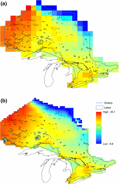
Comparison of daily mean temperature on July 15, 2008 from CCSM4 before (a) and after (b) downscaling


3.2 Transfer GCM precipitation data to CFSR grid points
3.2.1 Precipitation transformation
For daily precipitation downscaling, the construction of the gain Matrix is not straightforward.Precipitation is always positive, non-Gaussian and the number of days with precipitation are much shorter than the length of the time window (31 days for precipitation) for estimating the error covarianc matrix. Usually, both observed and modelled precipitations are transformed before downscaling. Lien et al. (2015) reviewed techniques used for precipitation transformation. Among these transformation methods, the logarithmic transformation has been widely used to the precipitation assimilation and downscaling (McLaughlin et al. 2002; Hou et al. 2004; Lopez 2011; Lien et al. 2015). Therefore, in this study we use it to transformate precipitation data:
where \({y^0}\) is the original daily precipitation, \(y\) is the transformed precipitation, and α (= 1) is a tunable constant added to prevent the singularity at zero precipitation \(\left( {{y^0}=0} \right)\). Thus, for days with zero (or no) precipitation days, y = 0. Downscaling is then conducted to the transformed precipitation. The final downscaled results are then transformed back using the following equation:
To avoid the underestimation of covariance, days without precipitation at both grid points were not used (Baigorria et al. 2007). Previous studies show that the spatial correlation during the frontal rainy season are characterized by a widely spread pattern in a northeast-southwest direction around locations which is perpendicular to the usual weather front paths. During the convective rainy season, correlations are characterized by small concentric patterns in which correlations decrease rapidly over short distances from each locations. For simplicity, we use 200 km as the threshold value for search type-A grid points. Similar to temperature, for some low resolution models, at least four Type-A GCM grid points at each of CFSR grid points should be selected for downscaling.
3.3 Bias correction
In present paper, we use the linear scaling method to correct biases in mean, and variation scaling method to correct biases in variance. These methods are simple and have been widely used in many downscaling studies (Teutschbein and Seibert 2012; Fang et al. 2015; Deng et al. 2016). For completeness, we provide the following brief descriptions on these methods.
3.3.1 Linear scaling of temperature
The analysed temperature is often corrected with help of an additive term based on the difference of long-term mean between observation and historical run data (Teutschbein and Seibert 2012; Lenderink et al. 2007; Fang et al. 2015), expressed by the following equation:
where \(X\) represents the variable to be corrected; \({\mu _m}\) represent the means; superscript d and 1 represents downscaling and first step of bias correction, respectively; subscript obs, hist and proj represent observation (reanalysis), historical runs and projection runs, respectively. Since most historical simulation data of CMIP5 GCMs end in 2005, there are only 25-year data that overlay with the CFSR data (1981–2010). So, we use the 25-year (1981–2005) mean of CFSR data to correct the bias in the mean of each GCM.
3.3.2 Variance scaling
In general, GCMs often underestimate the variance of temperature. Many extreme climate indices are based on daily temperatures (e.g., CDD, HDD, Tx30 and Tn20); the underestimated variance may lead to the estimated indices significantly depart from reality. Therefore, the variance should be further scaled. After using Eq. (8), we scale the standard deviation of the model anomalies with the following equation:
Eventually, the corrected data \(X_{{proj}}^{{d,2}}\) has the same mean and standard deviation as the CFSR data \(\left( {{X_{obs}}} \right)\) during the 25-year historical run period (1981–2005). This procedure is applied to temperature data month by month from 1981 to 2100.
3.3.3 Wet day precipitation bias correction
We use the same method used for temperature correction to correct biases in monthly and annual total precipitation. Daily precipitation, which mainly used to estimate some indices, such as R10mm, R20mm, 30-year return levels, etc., will be corrected with distribution fitting method. Since the indices are based on wet day (daily precipitation ≥ 1 mm) precipitation, in the present paper we focus on correction of wet day precipitation. The distribution fitting method has been used in downscaled CMIP3 precipitation correction (Deng et al. 2016). For completeness, the method is described below. Previous studies (e.g., Waggoner 1989; Watterson 2005) have demonstrated that the most preferred distribution to fit wet-day rainfall amounts is the 2-parameter Gamma distribution function:
where α and β are respectively the shape and scale parameters of the distribution. The expectation is E (= α × β). We use the 2-parameter Gamma distribution to fit wet-day precipitation at each grid point. The goal of precipitation bias correction is to make the model data and reanalysis data have the same total wet days for the reference period 1981–2005 and follow same distribution. This method adjusts the precipitation series at each of the 1552 grid points in Ontario by removing the bias in wet-day frequency and intensity. To achieve these goals, firstly, we determine a threshold \(\left( {{{\text{R}}_{\text{c}}}} \right)\) of wet days at each grid point for each ensemble member:
where \(F\) is the empirical cumulative density function (CDF), so \({F_{DS}}\) and \({F_{CFSR}}\) refer to the CDFs of downscaled and CFSR precipitation, respectively. Thus, the total wet days (daily precipitation ≥ \({{\text{R}}_{\text{c}}})\) of downscaled data exactly equals the total wet days (daily precipitation ≥ 1 mm) of CFSR data for the reference historical period (1981–2005). The next step is to adjust the intensity of wet-day precipitation to make the estimated expectation \(\left( {{{\text{E}}_{\text{m}}}} \right)\) of GCM data at a grid point equal that of the reanalysis data \(\left( {{{\text{E}}_{\text{o}}}} \right)\), i.e. \(\left( {{{\text{E}}_{\text{m}}}={{\text{E}}_{\text{o}}}} \right)\). Two steps are needed to get the adjustment coefficient \(\left( {r={r_1}{r_2}} \right).\) Firstly, we use the following formula to adjust the model wet day precipitation data:
where \({{\text{y}}^{\left( 1 \right)}}\) and \({\text{y}}\) are the model value after and before correction respectively, \({r_1}=\frac{{{{\varvec{E}}_{\varvec{o}}}}}{{{\mathbf{E}}_{{\varvec{m}}}^{{\left( 0 \right)}}}}\), \({\text{E}}_{m}^{{\left( 0 \right)}}={{\varvec{\upalpha}}}_{m}^{{\left( 0 \right)}} \times {{\varvec{\upbeta}}}_{m}^{{\left( 0 \right)}}\) and \({{\text{E}}_{\text{o}}}={{{\varvec{\upalpha}}}_{\text{o}}} \times {{{\varvec{\upbeta}}}_{\text{o}}}\) is estimated expectation of wet day precipitation of the model run and the CFSR for the overlap period (1981–2005). \({{\varvec{\upalpha}}}_{m}^{{\left( 0 \right)}}\) and \({{\varvec{\upbeta}}}_{m}^{{\left( 0 \right)}}\) are shape and scale parameter of model data respectively, \({{{\varvec{\upalpha}}}_{\text{o}}}\) and \({{{\varvec{\upbeta}}}_{\text{o}}}\) are the shape and scale parameters of CFSR data respectively, and the value 1.0 mm is standard threshold value of observed wet day. After using Eq. (10), the threshold of wet day of the model data \(\left( {{{\varvec{R}}_{\varvec{c}}}} \right)\) is replaced with 1.0 mm. Subsequently, the shape and scale parameters of the adjusted model data change from \({{\varvec{\upalpha}}}_{m}^{{\left( 0 \right)}}\) and \({{\varvec{\upbeta}}}_{m}^{{\left( 0 \right)}}\) to \({{\varvec{\upalpha}}}_{m}^{{\left( 1 \right)}}\) and \({{\varvec{\upbeta}}}_{m}^{{\left( 1 \right)}}\). Therefore the result from Eq. (12) should be further corrected using the following equation
where \({r_2}=\frac{{{{\varvec{E}}_{\varvec{o}}}}}{{{\mathbf{E}}_{{\varvec{m}}}^{{\left( 1 \right)}}}}\), and \({\mathbf{E}}_{{\varvec{m}}}^{{\left( 1 \right)}}={{\varvec{\upalpha}}}_{m}^{{\left( 1 \right)}} \times {{\varvec{\upbeta}}}_{m}^{{\left( 1 \right)}}\) is the estimated expectation of model wet day precipitation from Eq. (10). Finally, the estimated expectation of model data from Eq. (13), \({\mathbf{E}}_{{\varvec{m}}}^{{\left( 2 \right)}}={{\varvec{\upalpha}}}_{m}^{{\left( 2 \right)}} \times {{\varvec{\upbeta}}}_{m}^{{\left( 2 \right)}}\), is exactly equals to \({{\text{E}}_{\text{o}}}\). With this method, we can get \({{\text{R}}_{\text{c}}}\) and coefficient \(r={r_1}{r_2}\) at each grid point for each ensemble member. Then they are used to correct the wet-day daily precipitation amount for the projection periods.
3.4 Evaluation and validation
Two experiments are carried out to evaluate the downscaling method: (1) K-fold cross validation based on outputs from three historical runs for the 25-year base period (1981–2005) and (2) comparison downscaled data from the low resolution NCEP_Reanalysis_2 data with observations and ERA-Interim data.
3.4.1 Cross-Validation for the historical period
To evaluate the transfer method we proposed in this study (described in Sects. 3.1, 3.2), a five-fold cross-validation is carried out to test the downscaled outputs for the 25-year base period (1981–2005) from CCSM4, GFDL-ESM2M and CanESM2 historical runs (Kohavi 1995; Gutiérrez et al. 2013). We run the downscaling model 5 times. Each time, 5-year (1981–1985,1986–1990, 1991–1995, 1996–2000 and 2001–2005) data are used for testing, and the other left 20-year data are used for estimating the gain matrix. For comparison, the Inverse Distance Weighted (IDW) interpolation method is applied to generate the spatial distribution of daily data. IDW is widely used as a simple spatial downscaling method (Akinyemi and Adejuwon 2008; Mandal and Simonovic 2017) and is often used as the first step in some empirical downscaling methods as well, for example the QQ-mapping (Li et al. 2012) and the local intensity scaling (LOCI: Schmidli et al. 2006; Deng et al. 2016).
Evaluation is carried out using the 25-year averages of monthly mean for the four basic variables. Since the goal of the transfer function (1) is to add high resolution detail to CFSR grid points, large spatial scale variation are removed from the 25-year averages (of CFSR, IDW and EnOI data) by substracting the spatial running means prior to the comparison. The running mean at a CFSR grid point is estimated based on data at CFSR grid points within a 2.5° latitude × 2.5° longitude moving window which centered at the subject grid point. Then, the differences between the original data and the running mean of the CFSR, IDW and EnOI data (denoted respectively as \({Z_c}\), \({Z_I}\) and \({Z_E}\)) may represent the local climate information. The absolute errors of EnOI and IDW data are estimated by E1 (= \(\left| {{Z_E} - {Z_C}} \right|\)) and E2 (= \(\left| {{Z_I} - {Z_E}} \right|\)) at each of the 1522 CFSR grid points for Pr, Tm, Tx and Tn. Next, the difference between the errors (dE = E1–E2) are calculated. If dE < 0, the EnOI method outperforms the IDW method and vise versa. Finally, we can check if the EnOI method outperforms the IDW method based on the ratio of the number of points (N1) where dE < 0 to the number of points (N0 = 1522-N1) where dE ≥ 0. The ratio N1/N0 represents how better (N1/N0 > 1) or worse (N1/N0 < 1) is the EnOI method relative to the simple IDW method. The spatial averaged differences of error dE were compared as well.
3.4.2 Independent validation by comparing downscaled NCEP data with observations and ERA-Interim data
Since GCMs deal with climate rather than weather, it is inappropriate to compare the downscaled data from GCMs with observations day by day. To further evaluate the proposed downscaling method at multiple timescales, the low resolution NCEP_Reanalysis 2 data is downscaled to the CFSR grid points. Then, the downscaled data can be compared with station observations and another high resolution reanalysis data ERA-interim at daily scale.
3.5 Projection and uncertainty analysis
After daily temperatures and precipitation for the period 1981–2100 from 29 GCMs are downscaled and bias-corrected, some variables that represent climate averages and extremes are projected for 2050s and 2080s. The spreads of the multiple model ensemble are calculated to characterize the uncertaintiesin these variables (Knutti et al. 2010). In general, one would expect that larger (smaller) ensemble spread implies more (less) uncertainties in the projection (Hopson 2014). There are a few metrics of ensemble spread, such as ensemble standard deviation, mean absolute deviation, etc. In this study, the standard deviation (S) is used to measure the spread of the ensemble for the given projection ensemble \({\theta _i}\) (Hopson 2014):
where M (= 29) is the ensemble size, \(\tilde {\theta }\) denotes the ensemble mean.
4 Results
4.1 Validation of the proposed downscaling model
4.1.1 Comparing errors in monthly avarages of downscaled GCMs data
Two cross-validation mesures are applied to evaluate the EnOI downscaling method, the ratio N1/N0 and the difference in absolution error (E1–E0). Figure 5 shows the ratios (left) and differencs (right) for models CCSM4 (top panel), GFDL-ESM2M (middle panel) and CanESM2 (bottom panel), respectively. The ratio figures (Fig. 5a, c, e) clearly show that the EnOI method outperforms the IDW for Tm (black line) and Tx (red line) for all of the three GCMs for almost all months. The numbers of grid points where the EnOI generates smaller error doubled the numbers of grid points where the IDW generates small error for Tm and Tx during most months. For Pr, the EnOI performs much better than IDW in cold seasons for GFDL-ESM2M. There is no significant difference between the two methods for the other two GCMs. For Tn from CCSM4, at most grid points (N1/N0 > 2) the EnOI method performs better than the IDW method while the EnOI method performs better in cold months but worse in warm months. Consistent with the results of the ratios, the absolute errors (Fig. 5b, d, f) show the reduction of errors by EnOI relative to the IDW. Averaged over Ontario, errors from IDW are 0.5 – 3 mm for Pr, 0.2 – 0.4 °C for Tm, 0.2 – 0.7 °C for Tx and 0.2 – 0.4 °C for Tn. Generally, the maximum errors happen in summer months. From Fig. 5b, d, f, we can see that EnOI performs better in all months for Tm and Tx. For Pr and Tn the EnOI method perferms better than the IDW method for most months although the results are model dependent. The EnOI method has larger errors than IDW method in some summer months. In summary, the EnOI method performs much better than the IDW method at most grid points for most varibles from most analized GCMs. It is important to note that the EnOI generates much better Tm and Tx which are critical for climate impact studies. Spatially, the EnOI method performs better in northern areas for precipitation and better in mountainous southern areas for temperatures (not shown).

Variations of N1/N0 (left) and E1–E0 (right) of Pr (cyan), Tm (black), Tx (red) and Tn (blue) with month. The ratios N1/N0 are based on the number of CFSR grid points where the EnOI outperforms IDW (N1) to the left grid points (N0 = 1522–N1). The unit for (E1–E0) is °C for temperatures and mm for precipitation. The values of E1–E0 for precipitation had been multiplied by a factor 0.5 for easy visualization
4.1.2 Comparing errors in downscaled NCEP data
To assess the accuracy of the proposed downscaling technique, firstly NCEP Reanalysis-2 data are downscaled to CFSR grid points and after that the downscaled data are compared with ERA-Interim reanalysis. Comparison between observations at the 54 stations and the downscaled data at the corresponding closest CFSR grid points is performed as well. The spatial distribution of the 30-year mean from NCEP II, EC and DS data for annual total precipitation and annual mean temperature are shown in Fig. 6. It shows that the spatial distribution patterns of downscaled precipitation (bottom left panel), ERA-Interim data (central left panel) and that of original NCEP II data (top left panel) are similar. Some local features, which appear in ERA-data but miss in the NCEP II data, are observed in the downscaled data. For mean temperature (right panel of Fig. 6) the three data sets are very similar to each other. But we still could discern improvements in central and southern area generated by the downscaling method. Similar situations are observed in Tx and Tn (not shown). Figure 7 demonstrates the relation between the data from downscaling (DS) at 54 CFSR grid points and at the corresponding closest weather stations. It is observed that they have good linear correlation in general. At northern areas where mean Tm < 5.5 °C, downscaled Tm and Tn are higher than their corresponding observed values, and downscaled values of Tx are lower than observed Tx. In other area, the downscaled temperatures are around the observed ones. Almost at all grid cells, the downscaled precipitation amounts are smaller than observations at the corresponding closest stations. Downscaled precipitation is smaller than observation at almost all stations, except for several station in northern area. These biases are partly inherited from coarse NCEP II data and partly generated by the downscaling method because the interpolation procedure may smoothes small-scale spatial variability. They will be considered in the bias correction procedure.

Comparison between 30-year mean of NCEP (top), EC-interim (middle) and downscaled (bottom) total precipitation (left, unit: mm), average temperature(right, unit: °C)

Scatterplot of 30-year (1981–2010) average of daily mean (a), maximum (b) and minimum (c) temperature and annual total precipitation (d) downscaled from NCEP reanalysis II dataset versus 30-year averages at the 54 weather stations in Ontario
To summarize goodness-of-fit of the quantiles for daily data, the widely used Quantile–quantile plot (QQ-plot) method is used in this study. Figure 8 depicts QQ-plots of the downscaled quantiles against the observed quantiles of daily data at five selected stations. Points on a QQ-plot that fall on the diagonal line indicate that the downscaled and observed datasets come from a same distribution and, in this case, suggest that the downscaling procedure accurately captured the distribution of the local-scale daily data (Kirchmeier et al. 2014). Points on a QQ-plot that fall on the regression line indicate that there exists a good linear relationship between quantiles of the two datasets. Figure 8 demonstrates a relatively good fit for Tm, Tx and Tn at the stations. There is a very good linear relationship between the quantiles although some regression lines do not exactly match the diagonal line and there are departures at the upper-tail points and lower-tail points. The downscaled Tm and Tx is biased towards a slightly higher temperature at station b and e. This good relationship justify the application of the linear bias correction method for temperatures. The QQ-plot for precipitation shows that the downscaled data and observed data match very well for wet day precipitation less than 20 mm/day, but downscaling underestimate precipitation greater than 20 mm/day at four of the five stations (a–d), except at station e. As previously mentioned, the underestimation may be inherited from NCEP II precipitation and the interpolation procedure. Further correction will be conducted to reduce these systematic errors.

QQplot of daily temperature (Tm) in summer, daily maximum temperature (Tx) in July, daily minimum temperature (Tn) in January and wet day precipitation in a year at five weather stations: (a) 91.9°W, 50.117°N; (b) 84.783°W, 47.967°N; (c)78.733°W, 44.333°N; (d)82.95°W, 42.267°N; (e) 74.733°W, 45°N. The horizontal and vertical coordinates represents observation and downscaled data, respectively. The dashed red line is linear regression line between them and the diagonal line represent x = y
As mentioned above, the method proposed in Sects. 3.1 and 3.2 only transfers the variables from GCMs to CFSR grid points. It can not correct biases inherited from GCMs. Figure 9 displays biases in six varibles. As examples, only results from three models and ensemble mean are presented. It is observed that the CCSM4 model has large biases in all of the six variables. Temperatures (Tm, Tx and Tn) show warm bias in all of the three models and the 29-member ensemble (except Tx in GFDL-ESM2M) over Ontario. Precipitation shows dry bias at most locations. Since the CFSR data is considered as observation for bias correction, after using Eq. (8), the means of all models become the mean of CFSR (blue circles) which are much closer to the observed normals (the blue straight line). The differences between the observed normals and CFSR data are possibly due to the gridded CFSR values are linearly interpolated to the 54 weather stations, it is possible to introduce minor errors during the interpolation where specific local geographic conditions were not fully accounted for. Although the CFSR data is not real observation, it should be better than gridded data merely based on observation at conventional weather stations, especially in areas where the observational data is sparse, such as the majority of central to northern Ontario. This bias correction approach is conducted for the results from other ensemble members for current and future projections as well.

Scatterplot of 30-year (1981–2010) mean temperatures of three selected models (GFDL-ESM2M, CCSM4 and CanESM2), 29-member ensemble mean and CFSR versus 30-year averages at 54 weather stations in Ontario. The unit in the figures is °C
4.2 Projected Temperature and precipitation changes
Model-projected warming varies in space and time. Figure 10 shows spatial distribution of the 29-member ensemble mean of Tm, Tx, Tn and Pr in 1990s and corresponding projected changes in 2050s and 2080s. It is observed that the amplitude of warming increase from southwest to northeast. Averaged over Ontario, Tm, Tx and Tn will increase 3.9(6.5) °C, 3.5(6.0) °C and 4.3(7.1) °C in 2050s (2080s), respectively. These results are in good agreement with the conclusion of the recent dynamical downscaling study (Wang et al. 2015). This demonstrated that the downscaling approach in this study is capable of accounting for some impacts from local geophysical features as well as dynamical downscaling approaches using expensive regional climate models. The local geographic conditions (latitudes, land covers, topography, etc) significantly affect the temperature change amplitudes. The maximum increasing amplitudes in the northeastern area are much larger than the minimum increasing amplitude in the southwestern area. As temperatures increasing, some temperature related climate indices will significantly change as well. As temperature increasing, annual total precipitation is projected to increase in about 40 – 100 mm (1 – 10%) in 2050s and 80 – 150 mm (6 – 20%) in 2080s (Fig. 10i–k). These increases mainly happen in winter and spring (December, January and February) but summer (June, July and August) precipitation is projected to decrease in most area for 2050s and 2080s over Ontario (figures not shown). Averaged over whole province, precipitation will increase about 6 and 11% annually and 24 and 42% in winter for 2050s and 2080s, but decrease about 2 and 2% in summer.

Maps of the 29-member ensemble mean of mean (a–c), maximum (d–f) and minimum (g–h) temperatures, and annual total precipitation for periods 1981–2010 (left), and their change in 2041–2070 (middle) and 2071–2100 (right) relative to 1981–2010. Blue contours are boundary of lakes and the black lines are boundary of municipalities
4.3 Projected changes in indices
Figure 11 shows some derived variables and their changes, including cooling degree days (CDD), heating degree days (HDD), hot days (TX30) and cold days (TN20) in 1990s and their projected changes in 2050s and 2080s. Currently (1990s), only small parts of southern Ontario need energy for cooling in summer (Fig. 11a), while the province needs large amount of energy for heating (Fig. 11d); days with Tx > 30 °C (TX30) is less than 33 days in Ontario (Fig. 11h); and there are more than 50 days with Tn < − 20 °C in area north of 50°N and less than 10 such cold days in southwestern Ontario (Fig. 11k). As temperatures continue increase, more and more areas will need cooling in summer (Fig. 11b, c). The CDD will increase more significantly in the south than in the north. The HDD will significantly decrease with larger decreasing amplitude in the north (Fig. 11e, f) because of the bigger amplitude of temperature increase (Fig. 10). TX30 increase more significantly in the south than the north (Fig. 11i, j). TN20 decrease significantly in the north (Fig. 11l, m). Averaged over Ontario, HDD will decrease 1144 °C (18%) and 1802 °C (29%), and CDD will increase 151 °C (148%) and 324 °C (318%) in 2050s and 2080s, respectively. Tx30 will increase 15 (214%) and 34 days (486%), and Tn20 will decrease 16 (30%) and 27 days (51%) in 2050s and 2080s, respectively. As total precipitation increase, the events of heavy precipitation (R10mm) will also increase over most part of Ontario. This increasing trend is consistent with the conclusion drew based on downscaled data from CMIP3 A2 GCMs (Deng et al. 2016) using the General Linear Model (Katz 2010).

Maps of the 29-member ensemble mean of CDD (a–c), HDD (d–f), TX30 (h–j) and TN20 (k–m) for the scenario RCP8.5 in 1981–2010 (left) and their changes in 2041–2070 (middle) and 2081–2100 (right) relative to 1981–2010
4.4 Ensemble spread
Because the Earth’s climate system is characterized by multiple spatial and temporal scale, uncertainties do not usualy reduce at a single, predictable rate (Cubasch et al. 2013). The bias correction reduces the uncertainty inherent in the downscaled results. However, the corrected means do not complete overlap with the observed normal (Fig. 9). Ensemble spread is often used to measure such uncertainty. Figure 12 shows the spatial distribution of ensemble spread of Tm, Tx, Tn, Pr and the 5 associated indices in 2050s. It is observed that the spatial distribution patterns of Tm, Tx and Tn are very similar to each other (Fig. 12a–c). The spreads are large in the north and small in the south. The spread distribution of HDD and Tn20 (days with Tn < −20 °C) are similar. The spatial distribution of CDD and Tx30 are similar with small values in the northeastern Ontario where the CDD and Tx30 are small (Fig. 12a, h) and their changes are small as well (Fig. 12b, i). The spatial distribution patterns of these variables are similar to that in 2080s (not shown) but with larger values because the ensemble spread increase with time. Different from temperature, the spread in Pr are larger in southern area than in northern area due to the larger amplitude of total precipitation. The uncertainty in R10mm are large over mountain area in the central Ontario.

Projected ensemble spread of annual Tm (a), Tx (b), Tn (c), CDD (d), HDD (e), Tx30 (f), Tn20 (g), Pr (h) and R10mm (i) for 2050s
5 Summary and discussion
Dynamical and statistical downscaling are the two widely used methods to generate high resolution regional climate data. They have their advantages and disadvantages. How to take the advantages of these methods and relieve the negative impacts of their disadvantages is an evolving topic. This study proposed a hybrid method to construct downscaling models using outputs of GCMs and CFSR, based on the framework for EnOI. We say it is a hybrid-like method because it takes advantages of both an assimilation based statistical downscaling approach (cost effective) and a high-resolution reanalysis system (i.e. CFSR) with better consideration of impacts from local geophysical features.
We use the day to day seasonal cycle of the high resolution spatially consistent daily reanalysis data as background state; the difference between outputs of GCM and the background state is spatially distributed onto the reanalysis grid points by a transfer function. The transformation maps the variables between the nearby GCM grid points and the CFS grid points. The results show that this method is capable of downscaling the GCM daily data to local scale with fairly reasonable confidence. The first step in statistical downscaling methods is to transformate GCM data onto target stations or grid point. Differing from some tradition downscaling methods which directly interpolate GCM data to target locations only considering impacts of limited constant geographic factors (distance, elevation, slope, etc), we use temporal varying gain matrix that can reflect the temporal variation of the interactions between the atmosphere and many local geographic factors at the reanalysis data resolution. These interactions vary with time which are reflected by the reanalysis models such as the CFS through coupling component models for the climate system. Biases are further corrected using the widely used linear scaling approach.
To validate the downscaling model, two experiments are carried out, a five-fold cross validation and an independent data comparison. The cross validation results show that the proposed EnOI method significantly outperforms the simple IDW method for Tm and Tx at most grid points. But its performance for Pr and Tn is season and model dependent. In the independent data comparison experiment, the lower resolution reanalysis data are downscaled to higher resolution grid points and then compared with observations and another high resolution reanalysis data. The results demonstrate that the EnOI method is capable of keeping large scale pattern from the low resolution model (e.g., GCM) and adding local details from the high resolution model (e.g., RCM). The good linear relation between the quantiles of downscaled daily data and real observation justifies the bias correction methods that are used to downscaled GCM data. Using the same methods, near surface temperatures (Tm, Tx and Tn) of a 29-member CMIP5 GCM ensemble under the IPCC AR5 RCP8.5 scenario are downscaled in Ontario. The result shows that averaged over the entire province, annual mean temperature will increase by respectively 3.9 to 6.5 °C in 2050s (2041–2070) and 2080s (2071–2100) relative to 1990s (1981–2010). Annual average minimum (maximum) temperature increases faster (slower) than mean temperature. The temperature increases with larger amplitude in the north than the south. Lakes play significant rule in modifying the changing amplitudes. Cooling degree days (CDD) increase significantly in the south and heating degree (HDD) decreases significantly in north. Hot days (Tx > 30 °C) will increase in the province with maximum increase in southern Ontario, and cold days (Tn < −20 °C) will decrease with maximum decreasing in northern Ontario. The ensemble spreads are larger in the north than other areas for temperatures (Tm, Tx and Tn), HDD and Tn20. For CDD and Tx30, large spreads happen in southern Ontario where the large absolute values of these variables appear. As temperature continue increasing, precipitation will also increase in most part of the province with larger amplitude in the eastern area and larger uncertainty in the southern area. The heavy precipitation event will increase significantly as well.
Usually the EnOI method requires running dynamical models, but our novel downscaling does not need, therefore it is a more computational efficient method which keeps spatial consistence to certain extent. The transfer function (gain matrix) reflects the complicated interactions between geographic factors and the atmosphere.
The EnOI method can be easily applied to other high resultion data. If outputs from a high resolution RCM simulation were used to construct the transfer function, then the transfer function would vary with year as well. For example, we can use the output of a high resolution RCM to construct the gain matrices for downscaling practice. This could relieve the negative impact of traditional statistical downscaling methods caused by the stationarity assumptions in which relationships between large and local-scale processes will remain the same in the future. In this study, gain matrices are constructed for each variable (Tm, Tx, Tn or Pr) independently to consider the interaction between geographic conditions and the variable at the reanalysis resolution. As demonstrated, the method proposed in this paper obviously improved the traditional statistical downscaling by implicitly keeping spatial and inter-variable consistence, and is useful for generating large ensemble of high resolution downscaling climate projections; note that, this method does not explicitly account for the interactions among variables and this may impact the coherence among them; and this could be improved by constructing multivariate gain matrices in our future research. Though this method has some advantages of dynamical downscaling because it is constructed from high resolution reanalysis data, it is still a statistical method. The transfer matrix (gain) only changes with calendar days but does not change with years. As climate changes, the relationship between large scale change and small scale variation represented by the gain matrix may change as well. In the future, we will use high resolution dynamical downscaling results to construct the transfer matrix which will change with time (day and years), thus will relieve the negative effects of this problem.
To make the EnOI applicable to downscaling, some assumptions are made. For example, it is assumed that the outputs of GCMs as observations with error variance as a small portion (10%) of the diagonal of the background (i.e. CFSR) error covariance matrix and does not change with years. Despite the assumptions are necessary for this study, they seems too confident. In this study, the proposed EnOI method is compared only with a very simple IDW downscaling method. Further comparison with other available advanced statistical downscaling methods may be helpful to understand the advantages and disadvantages of the EnOI method; this will be part of our future work. We will also look into further improving the EnOI method, for example, by re-designing the background error covariance matrix and observation error covariance to make them more realistic.
References
Akinyemi FO, Adejuwon JO (2008) A GIS-based procedure for downscaling climate data for West Africa. Trans GIS 12(5):613–631
Armstrong L (2015) Mapping and modeling weather and climate with GIS. Esri Press, Redlands
Baigorria GA, Jones JW, O’Brien JJ (2007) Understanding rainfall spatial variability in southeast USA at different timescales. Int J Climatol 27(6):749–760
Benestad RE (2005). Climate change scenarios for northern Europe from multi-model IPCC AR4 climate simulations. Geophys Res Lett 32(17)
Braun M, Klaas T, Vieira E, Eng P (2015) Manitoba-minnesota transmission project historic and future clima te study
Carrega P (ed) (2013) Geographical information and climatology. Wiley
Casanova S, Ahrens B (2009) On the weighting of multimodel ensembles in seasonal and short-range weather forecasting. Mon Weather Rev 137:3811–3822
Chadwick P, Hume B (2009) Weather of Ontario. Lone Pine Publishing, UK, pp 112–141
Cheng CS, Campbell M, Li Q, Li G, Auld H, Day N, Comer N et al (2008a). Differential and combined impacts of extreme temperatures and air pollution on human mortality in south–central Canada. Part I: historical analysis. Air Qual Atmos Health 1(4):209–222
Cheng CS, Campbell M, Li Q, Li G, Auld H, Day N, Comer N et al (2008b) Differential and combined impacts of extreme temperatures and air pollution on human mortality in south–central Canada. Part II: future estimates. Air Qual Atmos Health 1(4):223–235
Chiotti Q, Lavender B (2008) In: Lemmen DS, Warren FJ, Lacroix J, Bush E (eds) Ontario; in from impacts to adaptation: Canada in a Changing Climate 2007. Government of Canada, Ottawa, pp 227–274
Cubasch U, Wuebbles D, Chen D, Facchini MC, Frame D, Mahowald N, Winther J-G (2013) Introduction.Climate Change 2013: The Physical Science Basis. In: Contribution of Working Group I to the Fifth Assessment Report of the Intergovernmental Panel on Climate Change [Stocker, Qin T.F., D., Plattner G-K, Tignor M, Allen SK, Boschung J, Nauels A, Xia Y, Bex V, Midgley PM (eds.)]. Cambridge University Press, Cambridge
Dee D, National Center for Atmospheric Research Staff (eds) (2015) Last modified 05 Aug 2015. The climate data guide: ERA-Interim. https://climatedataguide.ucar.edu/climate-data/era-interim. https://climatedataguide.ucar.edu/climate-data/era-interim#sthash.47AH4fWr.dpuf
Dee DP et al. (2011) The ERA-Interim reanalysis: configuration and performance of the data assimilation system. Q J R Meteorol Soc 137:553–597. doi:10.1002/qj.828
Deng Z, Tang Y, Wang G (2010) Assimilation of Argo temperature and salinity profiles using a bias-aware localized EnKF system for the Pacific Ocean. Ocean Modell 35:187–205. doi:10.1016/j.ocemod.2010.07.007
Deng Z, Tang Y, Freeland HJ (2011) Evaluation of several model error schemes in the EnKF assimilation: applied to Argo profiles in the Pacific Ocean. J Geophys Res Oceans (1978–2012) 116(C9). doi:10.1029/2011JC006942
Deng Z, Tang Y, Chen D, Wang G (2012) A time-averaged covariance method in the EnKF for Argo data assimilation. Atmos Ocean 50(sup1):129–145
Deng Z, Qiu X, Liu J, Madras N, Wang X, Zhu H (2016) Trend in frequency of extreme precipitation events over Ontario from ensembles of multiple GCMs. Climate Dyn 46(9–10):2909
Environment Canada (1998) Atmospheric environment service, climate research branch. Climate Trends and Variations Bulletin for Canada, Ottawa
Environment Canada (2012) Canadian climate normals 1981–2010
Evensen G (2003) The ensemble Kalman filter: theoretical formulation and practical implementation. Ocean Dyn 53(4):343–367
Fang G, Yang J, Chen YN, Zammit C (2015) Comparing bias correction methods in downscaling meteorological variables for a hydrologic impact study in an arid area in China. Hydrol Earth Syst Sci 19(6):2547–2559
Field CB, Barros VR, Mastrandrea MD, Mach KJ, Abdrabo MK, Adger N, Burkett VR et al (2014) Summary for policymakers. Climate change 2014: impacts, adaptation, and vulnerability. Part a: global and sectoral aspects. In: Contribution of working group II to the fifth assessment report of the intergovernmental panel on climate change, pp 1–32
Flato G, Marotzke J, Abiodun B, Braconnot P, Chou S, Collins W et al (2013) Evaluation of climate models. In: Stocker TF et al (eds) Climate Change 2013: The Physical Science Basis. Contribution of Working Group I to the Fifth Assessment Report of the Intergovernmental Panel on Climate Change. Cambridge University Press, Cambridge, pp 741–866
Gao L, Schulz K, Bernhardt M (2014) Statistical downscaling of ERA-interim forecast precipitation data in complex terrain using LASSO algorithm. Adv Meteorol 2014
Gaspari G, Cohn SE (1999) Construction of correlation functions in two and three dimensions. Q J R Meteorolog Soc 125(554):723–757
Gutiérrez JM, San-Martín D, Brands S, Manzanas R, Herrera S (2013) Reassessing statistical downscaling techniques for their robust application under climate change conditions. J Clim 26(1):171–188
Gutmann E, Pruitt T, Clark MP, Brekke L, Arnold JR, Raff DA, Rasmussen RM (2014) An intercomparison of statistical downscaling methods used for water resource assessments in the United States. Water Res Res 50(9):7167–7186
Hall A (2014) Projecting regional change. Science 346(6216):1461–1462
Hopson TM (2014) Assessing the ensemble spread–error relationship. Mon Weather Rev 142(3):1125–1142
Hou AY, Zhang SQ, Reale O (2004) Variational continuous assimilation of TMI and SSM/I rain rates: impact on GEOS-3 hurricane analyses and forecasts. Mon Weather Rev 132(8):2094–2109
Jarraud M (2008) Guide to meteorological instruments and methods of observation (WMO-No. 8). World Meteorological Organisation, Geneva
Kalnay E (2003) Atmospheric modeling, data assimilation and predictability. Cambridge University Press, England
Katz RW (2010) Statistics of extremes in climate change. Clim Change 100:71–76
Kirchmeier MC, Lorenz DJ, Vimont DJ (2014) Statistical downscaling of daily wind speed variations. J Appl Meteorol Climatol 53(3):660–675
Knutti R, Abramowitz G, Collins M, Eyring V, Gleckler PJ, Hewitson B, Mearns L (2010) Good practice guidance paper on assessing and combining multi model climate projections. In: Qin TFD, Plattner G-K, Tignor M, Midgley PM (eds) Meeting report of the Intergovernmental Panel on Climate Change Expert Meeting on Assessing and Combining Multi Model Climate Projections Stocker. IPCC Working Group I Technical Support Unit, University of Bern, Bern
Kohavi R (1995) A study of cross-validation and bootstrap for accuracy estimation and model selection. Ijcai 14(2):1137–1145
Law M, Collins A (2013) Getting to know ArcGIS for desktop. Esri Press, Redlands
Lenderink G, Buishand A, Deursen WV (2007) Estimates of future discharges of the river Rhine using two scenario methodologies: direct versus delta approach. Hydrol Earth Syst Sci 11(3):1145–1159
Li Z, Zheng FL, Liu WZ, Jiang DJ (2012) Spatially downscaling GCMs outputs to project changes in extreme precipitation and temperature events on the Loess Plateau of China during the 21st Century. Global Planet Change 82:65–73
Lien G, Kalnay E, Miyoshi T, Huffman GJ (2012) Effective assimilation of global precipitation. In: AGU Fall Meeting Abstracts (vol 1, p 0096)
Lien GY, Kalnay E, Miyoshi T, Huffman GJ (2015) Statistical properties of global precipitation in the NCEP GFS model and TMPA observations for data assimilation. Mon Weather Rev (2015)
Lopez P (2011) Direct 4D-Var assimilation of NCEP stage IV radar and gauge precipitation data at ECMWF. Mon Weather Rev 139(7):2098–2116
Mach K, Mastrandrea M (2014) Climate change 2014: impacts, adaptation, and vulnerability. In: Field CB, Barros VR (eds) vol 1. Cambridge University Press, Cambridge, New York
Mandal S, Simonovic SP (2017) Quantification of uncertainty in the assessment of future streamflow under changing climate conditions. Hydrol Processes 31(11):2076–2094
Maurer EP, Hidalgo HG (2007) Utility of daily vs. monthly large-scale climate data: an intercomparison of two statistical downscaling methods. Hydrol Earth Syst Sci Discuss 12:551–563
McLaughlin JF, Hellmann JJ, Boggs CL, Ehrlich PR (2002) Climate change hastens population extinctions. Proc Nat Acad Sci 99(9):6070–6074
Mesinger F, DiMego G, Kalnay E, Shafran P, Ebisuzaki W, Jovic D, Fan Y et al (2004) NCEP North American regional reanalysis. Am Meteorol Soc
Moss RH, Edmonds JA, Hibbard KA, Manning MR, Rose SK, Van Vuuren DP, Meehl GA et al (2010) The next generation of scenarios for climate change research and assessment. Nature 463(7282):747–756
NCEP-DOE AMIP-II Reanalysis (R-2), Kanamitsu M, Ebisuzaki W, Woollen J, Yang S-K, Hnilo JJ, Fiorino M, Potter GL (2002) 1631–1643, Bull Atmos Met Soc
Ning L, Riddle EE, Bradley RS (2015) Projected changes in climate extremes over the Northeastern United States. J Climate 28:3289–3310. doi:10.1175/JCLI-D-14-00150.1
Oke PR, Schiller A, Griffin DA, Brassington GB (2005) Ensemble data assimilation for an eddy-resolving ocean model of the Australian region. Q J R Meteorolog Soc 131(613):3301–3311
Pimpler E (2013) Programming ArcGIS 10.1 with Python Cookbook. Packt Publishing Ltd, Birmingham
Qi P, Cao L (2015) Establishment and tests of EnOI assimilation module for WAVEWATCH III. Chin J Oceanol Limnol 33:1295–1308
Rana A, Moradkhani H (2015) Spatial, temporal and frequency based climate change assessment in Columbia River Basin using multi downscaled-Scenarios. Climate Dyn 1–22
Saha S et al (2010) The NCEP climate forecast system reanalysis. Bull Amer Meteor Soc 91:1015–1057. doi: 10.1175/2010BAMS3001.1
Saha S et al (2013) The NCEP climate forecast system version 2. J Clim doi: 10.1175/JCLI.-D-12-00823.1 (early online release)
Sakov P, Sandery PA (2015) Comparison of EnOI and EnKF regional ocean reanalysis systems. Ocean Model 89:45–60
Schmidli J, Frei C, Vidale PL (2006) Downscaling from GCM precipitation: a benchmark for dynamical and statistical downscaling methods. Int J Climatol 26:679–689
Schmidli J, Goodess CM, Frei C, Haylock MR, Hundecha Y, Ribalaygua J, Schmith T (2007) Statistical and dynamical downscaling of precipitation: an evaluation and comparison of scenarios for the European Alps. J Geophys Res Atmos 112:(D4). doi:10.1029/2005JD007026
Schoof JT (2015) High-resolution projections of 21st century daily precipitation for the contiguous US. J Geophys Res Atmos 120(8):3029–3042
Srinivasan A, Chassignet EP, Bertino L, Brankart JM, Brasseurg P, Chin TM, Counillon F, Cummings JA, Mariano AJ, Smedstad OM, Thacker WC (2011) A Comparison of sequential assimilation schemes for ocean prediction with the HYbrid coordinate ocean model (HYCOM): twin experiments with static forecast error covariances. Ocean Modell 37(3–4):85–111
Szeto KK (2008) On the extreme variability and change of cold-season temperatures in Northwest Canada. J Climate 21:94–113
Terink W, Hurkmans RTWL, Torfs PJJF, Uijlenhoet R (2010) Evaluation of a bias correction method applied to downscaled precipitation and temperature reanalysis data for the Rhine basin. Hydrol Earth Syst Sci 14:687–703. doi:10.5194/hess-14-687-2010
Teutschbein C, Seibert J (2012) Bias correction of regional climate model simulations for hydrological climate-change impact studies: review and evaluation of different methods. J Hydrol 456:12–29
Waggoner PE (1989) Anticipating the frequency distribution of precipitation if climate change alters its mean. Agri For Meteorol 47(2–4):321–337
Wang W et al (2011) An assessment of the surface climate in the NCEP climate forecast system reanalysis. Clim Dyn 37:1601–1620
Wang X, Huang G, Liu J, Li Z, Zhao S (2015) Ensemble projections of regional climatic changes over Ontario. Canada J Climate 28(18):7327–7346
Watterson IG (2005) Simulated changes due to global warming in the variability of precipitation, and their interpretation using a gamma-distributed stochastic model. Adv Water Resour 28(12):1368–1381
Werner AT (2011) BCSD downscaled transient climate projections for eight select GCMs over British Columbia, Canada. Pacific Climate Impacts Consortium. University of Victoria, Victoria, p 63
Wood AW, Maurer EP, Kumar A, Lettenmaier DP (2002) Long-range experimental hydrologic forecasting for the eastern United States. J Geophys Res 107:1–15
Wood AW, Leung LR, Sridhar V, Lettenmaier DP (2004) Hydrologic implications of dynamical and statistical approaches to downscaling climate model outputs. Clim Change 62:189–216
Acknowledgements
The authors would like to thank the Ontario Ministry of Environment and Climate Change (MOECC) for its financial support to this study, although the content is solely the responsibility of the authors and does not necessarily represent the official views of the MOECC. We thank the two anonymous reviewers for their constructive comments and suggestions.
Author information
Authors and Affiliations
Corresponding author
Additional information
This research was funded by Ontario Ministry of the Environment and Climate Change, Canada.
Rights and permissions
About this article

Cite this article
Deng, Z., Liu, J., Qiu, X. et al. Downscaling RCP8.5 daily temperatures and precipitation in Ontario using localized ensemble optimal interpolation (EnOI) and bias correction. Clim Dyn 51, 411–431 (2018). https://doi.org/10.1007/s00382-017-3931-3
Received:
Accepted:
Published:
Issue Date:
DOI: https://doi.org/10.1007/s00382-017-3931-3