Nonparametric approach for uncertainty-based multidisciplinary design optimization considering limited data

Abstract

Uncertainty-based multidisciplinary design optimization (UMDO) has been widely acknowledged as an advanced methodology to address competing objectives and reliable constraints of complex systems by coupling relationship of disciplines involved in the system. UMDO process consists of three parts. Two parts are to define the system with uncertainty and to formulate the design optimization problem. The third part is to quantitatively analyze the uncertainty of the system output considering the uncertainty propagation in the multidiscipline analysis. One of the major issues in the UMDO research is that the uncertainty propagation makes uncertainty analysis difficult in the complex system. The conventional methods are based on the parametric approach could possibly cause the error when the parametric approach has ill-estimated distribution because data is often insufficient or limited. Therefore, it is required to develop a nonparametric approach to directly use data. In this work, the nonparametric approach for uncertainty-based multidisciplinary design optimization considering limited data is proposed. To handle limited data, three processes are also adopted. To verify the performance of the proposed method, mathematical and engineering examples are illustrated.

1 Introduction

In engineering design, the traditional deterministic design optimization model, which considers variables as deterministic values, has been successfully applied to reduce the cost while satisfying the system requirements. In the cases of complex and coupled systems comprising many disciplines, multidisciplinary design optimization (MDO) has been widely used to solve system design problems (Yi et al. 2008; Balling and Sobieszczanski-Sobieski 1996). As an advanced optimization technique, MDO can provide a synthetic optimum solution of the system while satisfying complicated and nonlinear design constraints and considering the potential synergistic effect of each discipline. In addition, with the improvement of technology and competition between products, the demand for higher reliability and robustness of products is a challenge (Taguchi et al. 1983; Nguyen et al. 2009). Previously, to guarantee the reliability and consider potential uncertainty, a marginal design was performed by employing a safety factor multiplied by an actual constraint. However, because such a safety factor was defined based on the intuition of a designer or by using empirical data, it might have been misestimated, with a low safety factor causing a function fault and performance failure, and high safety factor leading to over design, and in turn to increased cost (Elms 2004). However, there is no quantitative standard to define a safety factor. Hence, a quantitative method, rather than a qualitative method, is necessary to economically and effectively consider uncertainty and guarantee reliability. For this purpose, uncertainty-based design (UBD) has been explored (Lee and Park 2001; Rao 1992). In UBD, two design approaches can be adopted. One approach is robust design optimization (RDO), which improves robustness to find a non-sensitive solution, i.e., a robust solution, without eliminating the causes (Lee and Park 2001). The other approach is reliability-based design optimization (RBDO) including reliability analysis (RA), or the so-called uncertainty analysis in the optimization process; in this approach,the probability of a system output is estimated quantitatively and statistically such that the design requirement—the reliability or the failure rate—is satisfied (Rao 1992). These approaches can also be applied together for the simultaneous improvement of reliability and robustness. Recently, MDO and UBD methodologies were integrated, and the resulting method was named uncertainty-based multidisciplinary design optimization (UMDO) (Yao et al. 2011). UMDO was first proposed in the field of aerospace engineering, and it gained attention because of the need for the regulations for reliability and robustness of responses to be strictly guaranteed, even for complicated disciplines.

In the early stage of UMDO design, to apply uncertainty to the design, the constraints imposed on the design were reformulated with redefined factors instead of the ideal factors based on the marginal design, which guaranteed the safety of the system even when the system faced the worst possible combinations of uncertainties. With a high safety factor, the design and optimization are prone to reach a solution that is more conservative than a solution obtained using ideal factors. The method called worst-case design was first proposed in aerospace engineering, which is mainly focused on disciplines such as structural engineering, aerodynamics, and control (Parkinson et al. 1993). The worst-case design has been shown to be effective in various applications in non-complex problems; however, when the MDO system has many constraints and a trade-off relationship exists between these constraints, the result of the worst-case design is ineffective, or the design fails to find feasible solutions (Gu et al. 2000).

The key steps in UMDO research involve determining how to consider the uncertainty propagated between disciplines and how to quantify the system probability of failure calculation (Yao et al. 2011). In the conventional method, for the UMDO problem considering the coupling relationship of disciplines, the first-order Taylor series approximation is widely used to analyze system uncertainty with cross propagation between disciplines. In addition, the first-order reliability method (FORM) is employed to quantify the reliability of systems because of the simplicity of calculation and good approximation of performance functions using the first-order Taylor series approximation (Du and Chen 2005; Padmanabhan and Batill 2002).

In an MDA phase, because the traditional methods assume that uncertainty is regarded with only normal distribution, the variation in the parameters of a normal distribution becomes a convergence criterion. For example, when the variation in mean and standard deviation between a previous and current iteration is within a specified tolerance, the MDA phase is stopped. However, when the normal distribution cannot identify the phenomenon or when the parametric distribution is incorrectly estimated in an uncertainty modeling step, a serious error can occur, and this error can increase because of uncertainty propagation. Even in realistic experiments and environments, the uncertainty is limited because experiments or exploitations are limited by a cost problem or an environment problem. Thus, the error increases during the optimization process owing to wrong assumption. Therefore, a new UMDO without using continuous parametric distribution but directly adopting limited data should be developed.

In this paper, a nonparametric approach for UMDO is proposed to consider limited data directly. Because the parameters that represent a probability density function (PDF) are not used, a new MDA phase and uncertainty analysis phase are proposed for a nonparametric approach. The MDA phase consists of two steps including a data-transferring step and a convergence test step. In a nonparametric approach, because the limited data of variables is directly used, each discipline, experiment, or simulation should import a combination of the limited dataof each variable. Hence, as a data-transferring step, an auto-correlation sequence is employed to make limited samples uncorrelated before analyzing a discipline in every iteration. The Kolmogorov–Smirnov test (K-S test) is then applied for a convergence test step to measure the uncertainty propagation of coupled variables (Massey 1951). The K-S test calculates the maximum difference of empirical cumulative distribution functions (ECDFs) between previous and current iterations. An MDA phase is stopped if the difference is within the specified tolerance. Finally, a nonparametric uncertainty analysis based on the Akaike information criterion (AIC) is proposed (Akaike 1973). AIC is a method that selects the best-fitted distribution from several candidate distributions. To validate the performance of the proposed method, mathematical and engineering examples are provided. To verify the accuracy of the proposed method, the reliabilities of responses at the optimum design as obtained by the proposed method were compared with those obtained by Monte Carlo simulation.

2 Uncertainty-based design

As a pre-process for employing uncertainty-based design, input factors with uncertainty should be defined, and the uncertainties of each input factor should be classified. We can then explain conceptually how to quantify and measure the uncertainties of input factors.

2.1 Uncertainty classification

Uncertainty can be commonly classified as epistemic and aleatoric uncertainties (Scott et al. 2004; Thunnissen 2005; Sankararaman and Mahadevan 2011; Liang et al. 2015). The epistemic uncertainty occurs when a quantity has not been measured sufficiently or accurately because the effects of the uncertainty have been neglected in the model owing to (1) an assumption or lack of knowledge, (2) deliberate hiding of particular data, or (3) lack of information. The aleatoric uncertainty is representative of unknowns that differ each time in the same experiment, and is attributed to individual variations and randomness of the model or phenomenon. In real life applications, both types of uncertainties overlap. The intention of uncertainty quantification is to work toward reducing epistemic uncertainty because aleatoric uncertainty cannot be reduced.

In the case of epistemic uncertainty, it is difficult to obtain an accurate statistical model and to quantify it accurately. Therefore, in this study, we focused on the quantification of aleatory uncertainty. To reflect this uncertainty in the design process, it is necessary to determine whether the uncertainty depends on the design variables or on the design parameter.

When the outputs of a function of design variables and parameters are assumed as the response, this classification is required because the deviations in design variables directly affect the sensitivity of the response in terms of design sensitivity. That is, if the uncertainty that is dependent on design variables is changed, the actual design sensitivity of the responses includes the sensitivity of standard deviation in the uncertainty and the sensitivity of the design variables. For example, manufacturing uncertainty is included in the uncertainty that is dependent on the design variables such as the shape and size of a product. In addition, environmental uncertainties and the uncertainty of material properties are included in the uncertainty that is independent of the design sensitivity because they the material properties are related to the design parameters.

2.2 Uncertainty-based design optimization

As engineering fields have become increasingly more competitive, there is a demand for superior quality products in the industry. The uncertainties from the control or noise factors that a designer cannot control are caused by involuntary variations in performances. In this paper, two uncertainty-based design optimization (UDO) techniques are explained (Taguchi et al. 1983; Nguyen et al. 2009; Lee and Park 2001; Rao 1992). Unexpected deviations in performances, which are caused by uncontrollable uncertainty, reduce the quality of products and their competitiveness. Robust design has been developed to improve the quality of engineering products (Taguchi et al. 1983). Recently, this technology has been expanded to various design areas (Beyer and Sendhoff 2007; Lee et al. 2014). The optimum solution of robust design techniques has a unique advantage over the deterministic design techniques that do not consider the uncertainty of factors. In deterministic design, point 1 is considered to be the optimum solution—the minimum value in the design space, as shown in Fig. 1. However, if the factors have uncertainty, which is called the variation in the factor, point 1 can potentially violate the constraint. On the other hand, in robust design, point 2 is considered as the optimum solution that improves the performance and minimizes the variance of performance due to the variation in the factor, Δx. Thus, point 2 never violates the constraint under the uncertainty. This result is called the robust optimum.

Fig. 1

Concept of uncertainty-based design optimization

On the other hand, product failure under uncertainty is a significant problem. In practice, because nominal values of design variables are used in the design, half of the products face the risk of failure even if only one constraint is active. A safety factor defined by a designer or an engineer is employed in conventional design optimization, but an empirically defined factor can cause overdesigned products, and an incorrectly assumed safety factor also causes failure. Hence, the failure rate can be improved through statistically defined quantification of uncertainty and optimization techniques. This process is termed RBDO (Youn and Choi 2004; Cho et al. 2014). Figure 2 shows the difference between the deterministic solution of the conventional design optimization and an RBDO solution. The dotted lines for each solution indicate the variation caused by the uncertainty. Only RBDO solution shows feasibility under the uncertainty.

Fig. 2

Difference between the solutions obtained by the overestimated safety factor, that obtained by the wrongly assumed safety factor, and that considering uncertainty

Robust design is similar to RBDO because uncertainty is considered in their optimization processes. Nevertheless, robust design handles the objective function to improve quality, and RBDO converts deterministic constraint functions to statistical constraint functions through an optimization formulation. Thus, the two uncertainty-based design methods were integrated in recent studies to form reliability-based robust design optimization (RBRDO) (Tang et al. 2012; Jang et al. 2015).

3 Uncertainty-based multidisciplinary design optimization

MDO was developed for the engineering fields that focused on complex systems involving a number of disciplines or subsystems (Yi et al. 2008; Balling and Sobieszczanski-Sobieski 1996). Because the performance of a multidisciplinary system is driven not only by the performance of the individual discipline, but also by its interactions, MDO is necessary for designing complex systems. However, traditional MDO theories consider the design variables, such as material properties and manufacturing tolerance, as deterministic design variables and parameters, even though the design variables and parameters are not deterministic values but values with uncertainties in real design. The traditional MDO is inaccurate because it does not consider these uncertainties. To include the uncertainty, UDO and MDO are integrated as the parametric approach UMDO (Yao et al. 2011). A flowchart of the parametric approach for UMDO is shown in Fig. 3.

Fig. 3

Flowchart of the parametric approach for uncertainty-based multidisciplinary design optimization

System modeling involves organizing disciplines, optimization formulation, and defining design variables, objectives, and constraints. Thus, this step should be carried out properly to obtain a meaningful solution. After completing this process, optimization is performed until an optimum solution is achieved. Many optimization algorithms can be employed in this process. During the optimization process, design information for obtaining a feasible solution is transferred to an uncertainty analysis process. This process consists of two sub-steps: MDA and uncertainty analysis.

As shown in Fig. 3, MDA is applied to find converged coupled variables between disciplines. In the MDA phase of an UMDO problem, the key step is to quantify the uncertainty propagation for coupled disciplines and to determine the convergence of the uncertainty for coupling variables. First, for a multidisciplinary complex system, if the uncertainty propagation across disciplines is not quantified properly, it can make the uncertainty analysis difficult and inaccurate. In the parametric approach for UMDO, the Taylor series expansion-based method is employed to analyze quantitatively the uncertainty of coupled variables propagated through the interaction of subsystems. Second, running a multidisciplinary analysis of the complex system with coupled disciplines is time-consuming because such an analysis requires numerous iterations for obtaining the appropriate convergence of coupled variables. In the parametric approach for UMDO, the user decides whether they converged on the basis of the difference between the parameters of distributions of coupled variables in the previous iteration and the current iteration (Padmanabhan and Batill 2002). If the sum of their differences is within a certain tolerance, the MDA process is stopped, and the final parameters and outputs are used to obtain the reliability in the uncertainty analysis step. This convergence test step is mathematically formulated as shown in Eq. (1). The superscript “old” indicates the mean and standard deviations of a previous iteration, and the superscript “new” indicates those of the current iteration.

$$ \begin{array}{l}\left\Vert {\mu}_{y_{12}}^{new}-{\mu}_{y_{12}}^{old}\right\Vert +\left\Vert {\sigma}_{y_{12}}^{new}-{\sigma}_{y_{12}}^{old}\right\Vert \\ {}+\left\Vert {\mu}_{y_{21}}^{new}-{\mu}_{y_{21}}^{old}\right\Vert +\left\Vert {\sigma}_{y_{21}}^{new}-{\sigma}_{y_{21}}^{old}\right\Vert < tolerance\end{array} $$

(1)

After the MDA process, the effect of uncertainty should be evaluated to determine whether the system is safe. This step is called the uncertainty analysis. In the parametric approach for UMDO, mainly FORM (which approximates as a linearization of a first-order equation for a limit state function) is used to evaluate the reliability (Du and Chen 2005).

In uncertainty analysis process, coupled variables and responses are obtained by analyzing the disciplines. This process is repeated until the criterion of convergence for coupled variables with uncertainty propagation is satisfied as expressed in Eq. (1). The information obtained from the MDA process is used to quantify the uncertainty of the system. Finally, the optimization process is completed when the updated information of objectives and constraints obtained from the final step satisfies the requirements. However, with FORM, the accuracy of the reliability decreases as nonlinearity increases because it only employs first-order Taylor expansion. Moreover, it is difficult to apply FORM to non-normally distributed design variables and parameters even if they can be transformed to normal distributions, because errors arise during this process. Thus, there is the demand for a new method that does not require such an assumption for engineering applications that have many distributions and nonlinearity.

4 Nonparametric approach for UMDO

4.1 Theory preliminary

4.1.1 Definition of nonparametric approach in UMDO

The reliability is generally determined by tail distributions and the tail models of the most distributions are similar configuration. Thus, there are small errors to estimate the reliability in RBDO even though the selected distribution in parametric approach is not the best fitted distribution. Due to that reason, the parametric approaches in RBDO have been recognized as an efficient method. It is why previous UMDO techniques have been developed from RBDO techniques. However, the process of UMDO is quite different with it of RBDO due to the MDA. MDO have to do a repetitive inner process called as MDA, to obtain the coincident coupled variable. In contrast with RBDO, propagated uncertainty should be quantified in MDA of UMDO. As a qualitative criterion, parametric approaches use statistical moments of uncertainty expressed in a certain distribution such as a normal distribution. It does not focus on tail configuration and inaccurate distribution estimation makes the error of the MDA result propagated. Also, the distributions of coupled variables can be changed while the coupled variables are converged in MDA process. Consequently, these phenomena in UMDO cause an error in uncertainty analysis process, and the optimum design from the parametric approaches cannot guarantee the total system reliability. Therefore, anew UMDO method should be developed.

The key of UMDO is how to reduce an error in MDA process until the distribution of coupled variables between the previous and current iteration is coincided. One alternative is to directly use the uncertainty data of coupled variables in MDA process instead of using parameters. Only the data of coupled variables is dealt with in the MDA process until the data is converged without any assumption. It is why the proposed method is termed as nonparametric approach for UMDO. The use of nonparametric approach in MDA reduces the propagation of error by parametric estimation.

After MDA process, uncertainty analysis method is required to obtain the reliability. Monte Carlo simulation (MCS) method is widely used for sampling method. However, it is unable to apply to UMDO because it needs many samples for the accurate reliability. Also, if MCS using the insufficient data makes the uncertainty analysis process in Fig. 4 not converged due to the discontinuous reliability value. Thus, the estimation method for the insufficient data should be adopted. In this paper, Akaike information criterion (AIC) method which effectively estimates the best distribution type for the insufficient data is applied.

Fig. 4

Flowchart of nonparametric approach for uncertainty-based multidisciplinary design optimization

4.1.2 Definition of limited data

In the design process, the uncertainty data might be complete data or limited data to estimate distribution. However, the sample size which can be completed for estimation is unclear. And all the uncertainty data required for UMDO problem is unable to have complete data. Especially, the experimental data is form of limited data due to time and cost. In that case, it is necessary to directly use the limited data in UMDO without any processing, which is related to apply the nonparametric approach to UMDO process.

For the nonparametric approach, the appropriate amount of limited data is necessary. Because the uncertainties of all the design variables are combined in MDA process, the sample size of uncertainty data for all disciplines should be equal. In this paper, the number of limited data of all design variables is assumed to be the same. If the number of limited data of design variables differ, resampling techniques such as slice sampling and Markov chain Monte Carlo (MCMC) method should be applied (Neal 2003; Christophe et al. 2003).

4.2 Nonparametric approach procedure

As shown in Fig. 4, the nonparametric approach for UMDO consists of three parts. In the first part, the system modeling process involving system modeling and uncertainty modeling is carried out. The disciplines and the relationships between disciplines are investigated in the system modeling process. Then, the uncertainty of design variables or parameters is quantified in the uncertainty modeling process. In the second part, the optimization process, the optimization algorithm transfers a candidate design point to the uncertainty analysis process until it is converged. Lastly, uncertainty analysis process is performed as the third part. This process consists of MDA and uncertainty analysis, which is similar to the parametric approach for UMDO. In the MDA process, the limited data is directly used and outputs of them are calculated. Before analyzing each discipline, auto-correlation sequence is performed to retain the relation between the limited data of the coupled variables. The limited data of coupled variables is determined using the fixed point iteration method, and convergence is checked by the Kolmogorov-Smirnov test (K-S test) (Massey 1951). After the MDA process, uncertainty analysis is performed based on the pre-determined limited data of responses.

4.3 Auto-correlation sequence

If a discipline has more than two variables with uncertainty, responses of the discipline are influenced by relation between variables with uncertainty. In the proposed method, it is able to control the relation between variables with uncertainty because the uncertainty data is directly used. Figure 5 shows the relation between variables. Uncertainties indicated in Fig. 5a and b have a dependent relation with each other, and the relation of Fig. 5a is stronger than that of Fig. 5b. On the other hand, the samples are evenly spread in the domain in Fig. 5c have independent relation.

Fig. 5

Density shape of limited data according to correlation; (a) top-left, (b) top-right, (c) bottom

The methods to evaluate the relation between samples are widely known for the Pearson correlation coefficient, Spearman correlation coefficient, and Cronbach’s alpha. In this research, considering the size and type of data and the limited data, the Pearson correlation coefficient was used. It is calculated as shown in Eq. (2).

$$ r={r}_{xy}=\frac{{\displaystyle \sum_{i=1}^n\left({x}_i-\overline{x}\right)\left({y}_i-\overline{y}\right)}}{\sqrt{{\displaystyle \sum_{i=1}^n{\left({x}_i-\overline{x}\right)}^2}}\sqrt{{\displaystyle \sum_{i=1}^n{\left({y}_i-\overline{y}\right)}^2}}} $$

(2)

The Pearson correlation coefficient, γ, ranges from −1 to 1. The magnitude of the value indicates the degree of correlation, a value close to 1 or −1 indicates a strong correlation, and a value close to 0 indicates a weak correlation between the two data values.

In this research, this process is called “Auto-correlation sequence,” because it regulates the correlation between uncertainties of coupled variables. And it is performed in each discipline analysis to ensure an adequate response.

In a MDA procedure, the limited data of the coupled variable is determined through the analysis of other discplines. In the fully coupled problem, the limited data of the coupled variable is variated due to the analysis of other discipline until the coupled variable converges. Thus, the auto-correlation sequence is able to guarantee the relations between uncertainties of the variables before discipline analysis in every iteration. In case of independent relation, the method makes the sample set in forms of multi-variate normal distribution. Figure 6 shows how auto-correlation sequence is performed in the MDA process. This example has two coupled disciplines. Each discipline has three input variables, two design variables and one coupled variable. In the view point of nonparametric UMDO, the inputs have individual distributions due to its uncertainty as shown in Fig. 6. In the n ^th iteration, the uncertainties of design variables x ₁, x ₂ and coupled variable y ₂₁ ⁽ⁿ⁾ are used to analyze discipline 1.

Fig. 6

Auto-correlation sequence in multidisciplinary analysis

For analysis of discipline 1 at n ^th iteration, the number of data set should be analyzed. it is important to choose the combination of the data set, [x ₁, x ₂, y ₂₁]. In auto-correlation sequence, the correlation of data set is determined according to the prior information from correlation analysis. If the input data have correlation, the proposed method can control the correlation of data set. This is one of the advantages compared with parametric approaches in UMDO.

To obtain a response set, y ₁₂ ⁽ⁿ⁾, adequate auto-correlation sequence is carried out on the uncertainties of x ₁, x ₂, and y ₂₁ ⁽ⁿ⁾. Similarly, auto-correlation sequence between the data of x ₃, x ₄, and y ₁₂ ⁽ⁿ⁾is carried out before analysis of discipline 2 to obtain data set of y ₂₁ ⁽ⁿ⁺¹⁾. As shown in Fig. 6, the data of a coupled variable y ₂₁ ⁽ⁿ⁺¹⁾differs from that of y ₂₁ ⁽ⁿ⁾. Therefore, auto-correlation sequence is repeated in every iteration until the uncertainties of coupled variables,y ₂₁ ⁽ⁿ⁾ and y ₁₂ ⁽ⁿ⁾, are converged. The next chapter the method to check the convergence of the data of coupled variables is introduced.

4.4 Kolmogorov-smirnov test

In a fully coupled MDO problem, the coupled variables between the disciplines and their uncertainty distribution are unknown. The coupled variables are inputs for a discipline and are the same as the output of another discipline. The uncertainties of the variables propagate through these coupled relations in UMDO problems. In the nonparametric approach for UMDO, in which the uncertainty is discrete form such as that shown in Fig. 7, the uncertainties of coupled variables are also discrete form. Therefore, the uncertainties of coupled variables are variated with iteration and cannot be determined by a certain distribution such as the parametric approach. In this research, all information of variable uncertainty in MDA procedure exist in the discrete data forms, in the other words they are not expressed in certain parameter, which is nonparametric. For nonparametric, we have to check the convergence of the coupled variables over the iteration. There are many researches to check the distribution fitness for the specific data. However, we need to evaluate the difference between discrete data in n ^th iteration and in n + 1th iteration. It is quite different with distribution fitness. Thus, we need to propose a new criterion for checking the convergence of the uncertainty of coupled variables.

Fig. 7

Uncertainty propagation in the nonparametric approach

We give attention to the simplicity of the K-S test which is widely known for one of distribution check method (Massey 1951; Engmann and Cousineau 2011). The K-S test is also able to provide the maximum difference level between two discrete data. In this research, the data can be considered as converged if the sum of the test statistics of the coupled variables is less than the tolerance pre-determined by a user. Equation (3) shows the mathematical expression of an example of this convergence criterion. F indicates the cumulative mass functions of each data of coupled variables. The superscript “old” indicates the cumulative mass function of the previous step, and the superscript “new” indicates that of the current step.

$$ \begin{array}{l}D=\underset{y_{12}}{ \sup}\left|{F}_{y_{12}}^{new}\left({y}_{12}\right)-{F}_{y_{12}}^{old}\left({y}_{12}\right)\right|\\ {}\kern0.96em +\underset{y_{21}}{ \sup}\left|{F}_{y_{21}}^{new}\left({y}_{21}\right)-{F}_{y_{21}}^{old}\left({y}_{21}\right)\right|< tolerance\end{array} $$

(3)

4.5 Akaike information criterion-based uncertainty analysis

After system analysis, the limited data of performance functions can be obtained through the steps explained earlier. Because this limited data consists of relatively little data, it is difficult to evaluate the precise reliability of a performance function directly. Therefore, a technique is necessary to calculate the reliability of a limited performance data. In this research, the AIC-based uncertainty analysis is employed. This method estimates the PDF of limited data and calculates the reliability based on the CDF.

The AIC is a criterion that estimates the best-fitted distribution and its parameters for the specific limited data (Akaike 1973). It selects the best-fitted distribution from candidate distributions listed by a designer. It is defined as shown in Eq. (4).

$$ AIC=-2\left({f}_{ml}-{n}_{free}\right) $$

(4)

where f _ml is the maximum log likelihood of a candidate distribution, and n _free refers to the number of parameters of the candidate distribution. The distribution with the lowest AIC value is the best-fitted distribution among the candidate distributions. We considered seven types of distributions as shown in Table 1. Figure 8 shows the overall procedure of distribution estimation from limited data using AIC (Cho et al. 2014).

Table 1 Types of the candidate distributions

Fig. 8

Distribution estimation by using the AIC

From the estimated distribution determined through AIC, the reliability can be calculated by integrating the PDF of the best-fitted distribution. The mathematical expression for this calculation is shown in Eq. (5).

$$ \begin{array}{l}R={\displaystyle {\int}_{-\infty}^{x=0}{f}_{\mathrm{best}\ \mathrm{fitted}}\left(x|\theta \right)dx}\\ {}\kern1em =F\left(0|\theta \right)\end{array} $$

(5)

5 Examples

Proposed method directly uses not a distribution assumption but limited data in MDA. The mathematical examples are used to show weakness of parametric approach compared with nonparametric approach in case of wrongly estimated distribution under UMDO problem. The accuracy of optimum results in two methods is compared with MCS result of each optimum point. Also, design of pilot miner system under deep-sea environments is applied to demonstrate the effectiveness of proposed method in real applications.

5.1 Mathematical examples

In order to demonstrate the performance of the proposed approach, mathematical examples are considered, and three methods are compared: deterministic approach, parametric approach, and nonparametric approach. As mathematical examples, two coupling problems between disciplines are selected for comparison. One is an uncoupled problem and the other is a fully coupled problem. Uncoupled problem is regarded as RBDO problem, not UMDO problem. The reason to choose these two problems is to check the difference between UMDO and RBDO when the parametric approach has ill-estimated distribution.

In addition, these problems are classified as two cases. One case considers the normally distributed uncertainty and the other case considers non-normally distributed uncertainty. Totally, four cases problems are solved to identify how wrongly assumed parameters influence on the accuracy of the reliability at the optimum.

• Example 1. Two-variable problem (Youn et al. 2005).

  $$ \begin{array}{l}\underset{X}{\mathrm{Min}}\kern1.08em {\mu}_{f(x)}\\ {}\ \mathrm{s}.\mathrm{t}.\kern1.44em {G}_1(X)= \Pr \left[{g}_1(X)\le 0\right]\ge 0.9772\\ {}\kern2.16em {G}_2(X)= \Pr \left[{g}_2(X)\le 0\right]\ge 0.9772\\ {}\kern2.16em {G}_3(X)= \Pr \left[{g}_3(X)\le 0\right]\ge 0.9772\\ {}\mathrm{where}\kern0.96em f(x)=-\frac{{\left({x}_1+{x}_2-10\right)}^2}{30}-\frac{{\left({x}_1-{x}_2+10\right)}^2}{120}\\ {}\kern2.28em {g}_1(X)=1-\frac{X_1^2{X}_2}{20}\\ {}\kern2.28em {g}_2(X)=-1+{Y}^2+{Y}^3-0.6{Y}^4+Z\\ {}\kern2.28em {g}_3(X)=1-\frac{80}{\left({X}_1^2+8{X}_2+5\right)}\\ {}\kern2.28em Y=0.9063{X}_1+0.4226{X}_2-6\\ {}\kern2.28em Z=0.4226{X}_1-0.9063{X}_2\\ {}\kern2.04em \end{array} $$

  (6)

  The first problem is an RBDO problem with uncoupled subsystems between disciplines. And it has two design variables and three constraints. It is difficult to solve this problem owing to the high nonlinearity of the constraints. In Ex. 1–1, the uncertainties of design variables are assumed as normal distribution as expressed in Eq. (7).

  $$ \begin{array}{l} Ex\kern0.24em 1-1\\ {}{X}_1\sim N\left({\mu}_{X_1},0.32\right),\kern0.24em 0\le {\mu}_{X_1}\le 10\\ {}{X}_2\sim N\left({\mu}_{X_2},0.32\right),\kern0.24em 0\le {\mu}_{X_2}\le 10\\ {}X=\left[{X}_1,{X}_2\right]\end{array} $$

  (7)

  The optimum results are listed in Table 2. The results of the parametric approach and nonparametric approach show that the results of them are converged to similar design points. For each approach, the optimum solution is validated by using MCS. The results show that the nonparametric approach has less error than the parametric approach, but there are no significant differences.

  Table 2 Results for example 1-1

  $$ \begin{array}{l} Ex\kern0.24em 1-2\\ {}{X}_1\sim beta\left(2,5\right)-0.2857+{\mu}_{X_1},\kern0.24em 0\le {\mu}_{X_1}\le 10\\ {}{X}_2\sim gamma\left(3,0.1\right)-0.2996+{\mu}_{X_2},\kern0.24em 0\le {\mu}_{X_2}\le 10\\ {}X=\left[{X}_1,{X}_2\right]\end{array} $$

  (8)

  The same problem in ex 1–1 is considered under the assumption of non-normally distributed uncertainty for design variables. As shown in Table 3, the parametric and nonparametric approaches provide similar solutions, while the deterministic approach does not guarantee the reliability because the it does not consider the uncertainty of design variables. Compared with MCS at each optimum, the nonparametric approach shows less error than the parametric approach for G ₁, and both approaches show almost the same reliability for G ₂.

  Table 3 Results of example 1-2

• Example 2. Normal distribution: three-variable problem (Park 2006)

  $$ \begin{array}{l}\underset{\mu_1,{\mu}_2,{\mu}_c}{\mathrm{Min}}\kern1.08em f={f}_1+{f}_2={\left(E\left[{Z}_1^{nc}\right]-0.5\right)}^2+{\left(E\left[{Z}_2^{nc}\right]-0.5\right)}^2\\ {}\mathrm{s}.\mathrm{t}.\kern1.92em {G}_1(X)= \Pr \left[1.0-{Z}_1^{nc}\le 0\right]\ge 0.9772\\ {}\kern2.52em {G}_2(X)= \Pr \left[1.0-{Z}_2^{nc}\le 0\right]\ge 0.9772\\ {}\mathrm{where}\kern1.08em {Z}_1^{nc}=\left({B}_1-2.5\right)+\left({B}_c-2.0\right)-0.5{Z}_2^c\\ {}\kern2.52em {Z}_1^c=\left({B}_1-2.5\right)+\left({B}_c-2.0\right)-0.4{Z}_2^c\\ {}\kern2.52em {Z}_2^{nc}=\left({B}_2-3.0\right)+\left({B}_c-2.0\right)-0.7{Z}_1^c\\ {}\kern2.52em {Z}_2^c=\left({B}_2-3.0\right)+\left({B}_c-2.0\right)-0.6{Z}_1^c\end{array} $$

  (9)

  The second problem is an MDO problem and a fully coupled problem between disciplines. It is selected to show the differences in the results of the MDA process when disciplines are fully coupled. Monte Carlo simulation (MCS) is used for validating each method, and the accuracy of system reliabilities at optimum results of each method are validated. In example 2–1, the uncertainties of all design variables are assumed to be normally distributed.

  $$ \begin{array}{l}{B}_1\sim N\left({\mu}_1,{0.5}^2\right),\;{B}_2\sim N\left({\mu}_2,{0.5}^2\right),\;{B}_c\sim N\left({\mu}_c,{0.5}^2\right)\\ {}0.0\le {\mu}_1,{\mu}_2,{\mu}_c\le 10.0\end{array} $$

  (10)

  Table 4 lists the results of each approach; all results have a small error of reliability as compared to MCS at the optimum points. The parametric and nonparametric approaches show similar optimum points and the reliability.

  Table 4 Results of example 2-1

  $$ \begin{array}{l}\left({B}_1+0.8862-{\mu}_1\right)\sim wbl\left(1,2\right)\\ {}\left({B}_2+2-{\mu}_2\right)\sim gamma\left(2,1\right),\;\\ {}\left(-{B}_c+0.2+{\mu}_c\right)\sim beta\left(0.5,2\right)\\ {}0.0\le {\mu}_1,{\mu}_2,{\mu}_c\le 10.0\end{array} $$

  (11)

  In example 2–2, a solution to the UMDO problem, which has a formulation as shown in example 2–1, is determined by adjusting non-normally distributed uncertainties such as Weibull, gamma, and beta distributions for design variables. The results in Table 5 show that the nonparametric approach presented similar reliabilities at the optimum points and that the parametric approach has relatively large error.

  Table 5 Results for example 2-2

5.2 Result of mathematical examples

In the parametric approach, the uncertainties of these coupled variables are assumed as normal distribution, which results in a large error in the MDA process. From examples 2–1 and 2–2, it is seen that if the uncertainties of coupled variables have non-normal distributions, the optimum solution obtained by the parametric approach is inaccurate because of its assumption. Further, the nonparametric approach provides better accuracy than the parametric approach for non-normal distributed uncertainty as shown in Fig. 9.

Fig. 9

Error comparison between parametric and nonparametric in mathematical examples

5.3 Engineering example: design of pilot miner system

Deep-sea manganese nodules that have been found on the seafloor contain many types of metals such as manganese, nickel, copper, cobalt, and rare-earth elements (Ku and Broecker 1969). They are economically valuable and are collected using the deep-sea mining system shown in Fig. 10. A pilot miner designed for collecting manganese nodules is an integrated system that includes the collector, the crawler, and the chassis structure (Hong et al. 2010). It collects manganese nodules while traveling on the cohesive soft soil of the deep-sea floor in the KODOS area, which is about 5000 m deep. Mining systems involve a variety of design requirements. Hence, the deep-sea mining system cannot be separately designed. Therefore, these design requirements necessitate the application of MDO (Lee et al. 2012; Cho et al. 2013).

Fig. 10

Schematic diagram of an integrated mining system

Meanwhile, the performances of the pilot miner are affected by noise parameters such as deep-sea environment parameters. In particular, the variations in oceanic current, shear stress, and steering ratio of the deep-seabed affect the travel stability, and the environment can bring about an unexpected change in travel stability. Moreover, a number of couplings occur among subsystems. For example, velocity is an input variable for the dynamic analysis of the crawler and a primary design variable of the collector. Thus, we should consider these coupled relationships for the design optimization of the pilot miner system using UMDO (Muro 1983; Lee et al. 2007).

Out of the many environmental variables, we select two, namely, steering ratio and shear strength. The shear strength of the deep-seabed is the most significant variable in the optimization of the test miner (Choi et al. 2010). Data of the noise variables were collected through exploration using a multiple corer (MC) with 9.5-cm diameter and a length of 60 cm between 1997 and 2006 in the KODOS area (Lee et al. 2006). The shear strength data of 117 samples as shown in Fig. 11 were used in this research (Choi et al. 2011). The steering ratio is assumed to have an exponential distribution with a specific range for operation because the pilot miner system spends most of the time traveling straight for collecting manganese nodules.

Fig. 11

Probability density obtained from the experiment data and histogram of the shear stress of the deep seabed at 10-cm depth

• 1) Frame

  The chassis structure supporting the vehicle system must be strong and stiff enough to maintain its shape under pressures of approximately 500 bars of the deep-sea and must be able endure any handling procedures such as launch and recovery of the miner. For the chassis structure, a structural analysis model was developed to evaluate the natural frequencies and structural strength using a commercial finite-element program, ABAQUS. For the boundary condition for structure analysis, the launch and recovery system (LARS)was considered because the water weight, acceleration of the cable required to recover, and the weight of the miner affect the total weight. The frame is illustrated in Fig. 12.

  Fig. 12

  

  Finite element model and its parameters for a structure of a pilot mining robot system

• 2) Crawler

  The pilot miner for collecting deep-sea manganese nodules must run stably on the cohesive soft seabed while collecting the manganese nodules. The traffic-ability of the crawler to move on cohesive soft soil depends strongly on the proper driving resistance. The driving resistance is directly related to the shear stress of the deep-sea soil (Chi et al. 1999). Further, a rigid-body model of the crawler is used to execute the dynamic simulation as fast as possible; the design variables for the model are shown in Fig. 13. The mean values of steady state were adopted to represent the responses of dynamic simulation. To evaluate the mobility of the traveling vehicle, four responses are considered: pitch angle (θ _pitch ), vertical sinkage (δ _z ), slip rate of track (slip), and drag velocity (V _g ).

  Fig. 13

  

  Design variables of the tracked vehicle part of the pilot robot mining system

• 3) Collector

  A collector is mounted in front of the self-propelled mining vehicle system, and it collects mineral resources from the ocean floor as illustrated in Fig. 14. In this research, we adopted the Coanda nozzle type, which floats manganese nodules from the deep-seabed by using the principle of a pressure drop in the jet flow through a rounded surface (Murakami et al. 1992). It is easy to operate and to transfer the manganese nodules, but the region between the collecting device and the deep-seabed is very sensitive. Thus, it is necessary to maintain certain distance between the collecting device and the deep-seabed and to optimize the curvature of the collecting plate, flow rate, and the nozzle shape for collecting efficiency (Murakami et al. 1992). Figure 15 presents the layout of the collector developed in our research. For robust operation under irregular ground conditions, a certain distance should be maintained between the ground and the collector plate while collecting the manganese nodules. In addition, lift force is one of the essential design requirements for ensuring sufficient collection. However, if the distance between the ground and the collector plate is large, the lift force is inefficient. This causes problems that make it difficult for the optimization method to find a feasible solution. Finally, the nozzles have a limit velocity even if the inflow of the water jet per unit time increases. Therefore, it is necessary to observe the limit velocity at the nozzles for efficient collection.

  Fig. 14

  

  Configuration of the collector of the pilot mining robot system

  Fig. 15

  

  Design variables of collector part of pilot mining robot system

• 4) Framework and formulation of pilot miner system

  Low power consumption of the total system is one of the essential design requirements. For this purpose, the scales of the mining vessel and the power cable system are determined. As the power consumption increases, the cost to install, operate, and maintain the system also increase exponentially. Thus, low power consumption of the crawler and the collector is considered as the objective of the design optimization.

  For the total pilot miner system, 13 design variables are defined. Among the 13 design variables, three are defined as common design variables that are used in all disciplines. They are the length of tracked vehicle (L), outer track span (B ₂ ), and distance ratio from the real centroid of buoyancy (R _b ). Six design variables are defined only for the frame: shell thicknesses of six parts of the frame. Four design variables are defined only for the collector: inflow water jet per unit time (Q), distance between the nozzle and ground (d), height of the nozzle from ground (h), and curvature of take-off plate (R).

  The coupling between each system should be investigated to formulate the problem. Since a collector picks up manganese nodules using the Coanda jet flow, the distance between the collector plate and ground (D _{take off} ) is important in the design. It can be affected by vertical sinkage (Sinkage) and pitch angle (Pitch) and also by the height of the collector plate (d). In addition, the track velocity (V _t ) can affect both the collector and the crawler considerably. The distance between the collector plate and the ground is coupled with vertical sinkage, pitch angle, and height of the collector plate. Further, drag velocity (V _d ) is coupled with slip rate (slip) and track velocity. These interactions are as follows:

  $$ \begin{array}{l}{D}_{take\; off}=d-\left[\frac{L}{2}\cdot Pitch+ Sinkage\right]\\ {}{V}_d=\left(1- slip\right)\cdot {V}_t\end{array} $$

  (12)

  According to the definitions of the design variable, environmental variable, and relationship between the disciplines, a system diagram of the pilot miner system was constructed as shown in Fig. 16. Thirteen design variables and two environmental variables were directly used in the analysis of disciplines. The response of frame analysis, that is, the weight of the pilot miner (W), is a coupled variable necessary for analyzing crawler discipline. Similarly, slip, sinkage, and pitch are coupled variables related to the crawler and collector discipline. Thus, the deep-seabed pilot miner system with 13 variables and 6 constraints is formulated as follows:

  $$ \begin{array}{l}\underset{\mathbf{X}}{\mathrm{Min}}\kern4em f\left(\mathbf{X}\right)={E}_{Crawler}\left(\mathbf{X},\mathbf{P}\right)+{E}_{Collector}\left(\mathbf{X},\mathbf{P}\right)\\ {}\mathrm{s}.\mathrm{t}.\kern4.21em {G}_j\left(\mathbf{X}\right)= \Pr \left[{g}_j\left(\mathbf{X},\mathbf{P}\right)\le 0\right]\ge 0.9772,\kern0.36em j=1\kern0.36em to\kern0.24em 7\\ {}\mathrm{where}\kern2.04em \mathbf{X}=\left[{B}_2,{R}_b,L,{T}_1,{T}_2,\dots, {T}_6,Q,h,R,d\right]\\ {}\kern5.75em \mathbf{P}=\left[{S}_r,\tau \right]\\ {}\kern3.86em \mathbf{g}\left(\mathbf{X},\mathbf{P}\right)=\left[{g}_1,{g}_2,{g}_3,{g}_4,{g}_5,{g}_6\right]\\ {}\kern6.82em =\left[{\omega}_1,{\sigma}_{\max },{D}_{take\; of f},{f}_{lift},{\overset{.}{M}}_{collector},{V}_{nozzle}\right]\\ {}\kern3.75em {\overset{.}{M}}_{collector}={f}_{lift}\times {V}_d\times \#\; of\; nodules\; per\; unit\; meter\end{array} $$

  (13)

  Fig. 16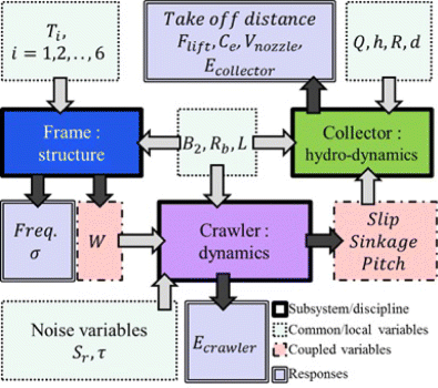

  

  Diagram of the pilot miner system

5.4 Result of engineering example

In this study, optimization was performed using the commercial program MATLAB. Sequential quadratic programming (SQP) was adopted as an optimization algorithm. As listed in Table 7, the initial design was infeasible owing to probabilistic constraints. As a result, all constraints were satisfied at the solution when the optimization of the proposed method is achieved. We can derive the UMDO result from the objective function—the total power consumption was decreased by about 14.1 % while all deterministic and reliable design constraints were satisfied. The results of UMDO are summarized in Tables 6 and 7. The design variables are expressed relative to the initial design between the lower and upper bounds, and responses are normalized to each constraint value.

Table 6 Comparison of optimization result: design variables

Table 7 Comparison of optimization result: Objective function and constraints

As listed in Table 7, the deterministic constraints of the initial design and deterministic MDO result are feasible, but probabilistic constraints do not satisfy the target reliability of 0.9772. However, the results of both the UMDOs, parametric and non-parametric, satisfy the feasibility of deterministic constraints and the target reliability of probabilistic constraints. At each optimum point of the UMDO solution, the reliability of probabilistic constraints was verified through Monte Carlo simulation. The solution of the parametric UMDO result had a maximum relative error of 13.4 %, but non-parametric solution had a maximum relative error of only 1.02 %. This is attributed to the non-normality of the coupled variable. As shown in Fig. 17, it is difficult to express the shapes of the histogram of the coupled variables as normal distributions.

Fig. 17

Histograms of coupled variables of the pilot miner: pitch, sinkage, and slip

6 Conclusion

This paper proposes a nonparametric approach for UMDO, which utilizes limited data of variables. The proposed method includes methods to find the optimum combination of limited data and perform the convergence check of coupled variables and reliability analysis through limited data.

• 1. In order to input independent limited data into different disciplines, it is necessary to find the optimum combination of limited data as a set of data. Since limited data includes many combinations, a method that finds the best set based on the correlation of the design variables preferred by the designer is proposed. The proposed method finds the optimum data set as the limited data changes, and this method only changes the combination of variables without causing any loss of information.

• 2. The MDO system aims to find the design point where all coupled variables converge. This aspect is the same in the nonparametric approach for UMDO. The proposed method, which directly uses the limited data, checks the convergence of the entire limited data because the coupled variables in the MDO system also include limited data. In this study, the convergence of the coupled variables was checked using the K-S test that minimizes the maximum error between the probabilities of two empirical CDFs based on the i-1th and ith coupled variables. The efficiency of convergence was enhanced because the method used only the probability, which is a normalized value.

• 3. The responses obtained after the MDA process are in the form of limited data. Therefore, it is impossible to apply the reliability analysis technique based on the parametric approach. In this study, the AIC method, which was developed to determine the best-estimated distribution in statistics, was applied as a reliability analysis technique. This method is not based on any assumption since it directly uses limited data. Further, it is easy to implement, and its result is robust to nonlinearities of responses.

The proposed nonparametric approach, which is divided into three detailed methods, is a different paradigm for presenting UMDO. The parametric approach for UMDO simply performs an additional analysis in the deterministic MDO method to estimate system reliability; the proposed method solves many of the problems of the present method, such as limitation of distributions, error amplification and convergence problems, and inefficiency when the number of design variables increases. The advantages of the proposed method are as follows:

• 1. The present parametric approaches for UMDO assume that the design variables are normally distributed. When the assumption of distribution is not appropriate, the errors increase. In the MDO system, when uncertainty propagation is incorrectly estimated, errors propagate, leading to inaccurate design. The proposed method is more effective because it directly utilizes the limited data of variables and has no limitations of distributions.

• 2. The most critical issue in the previous UMDO was uncertainty propagation in MDA. When nonlinearity exists, the previous methods that calculate the mean and standard deviation of coupled variables using Taylor series expansion can be inaccurate. The proposed method has no loss of limited data in MDA because it uses the limited data of the coupled variable, and thus, it allows more accurate design than that possible by previous methods.

• 3. The first order Tayler series expansion is a time-consuming process when the number of coupled variables increases. The proposed method is efficient when the number of coupled variables is large because it can independently extract the limited data of a coupled variable.

• 4. The convergence of the deterministic MDO method is checked by means of the changes in the coupled variables, but in the present UMDO, the convergence of the coupled variable is calculated as the sum of the change of mean and standard deviation. The increase in parameters causes low convergence and increased computational cost. The proposed method utilizes the K-S test to guarantee the convergence because the test employs only one parameter. This parameter is also a probability value, which is a normalized value regardless of the range of the coupled variable.

• 5. The accuracy is guaranteed because the method directly applies limited data without manufacturing the information. In previous parametric approaches for UMDO, several steps such as the determination of design variable distribution, extraction of information of coupled variable in MDA, and the assumption of normal distribution for coupled variable and constraints are needed. In this study, the only assumption needed is that the assumption of an optimal distribution among candidate distributions in the reliability analysis; thus, there is less loss of information.

• 6. In the Taylor series expansion and reliability analysis in the previous methods, as the number of design variables increases, the computational cost increases. This makes the method less applicable since MDO has many design variables. Because the proposed method does not use design sensitivity in the uncertainty propagation and reliability analysis, the number of design variables has less influence. The accuracy and computational cost may change with the amount of limited data, which can be controlled by the designer.

In this paper, a nonparametric approach for UMDO is proposed, and its advantages are analyzed. As mathematical examples, two coupling problems between disciplines are selected for comparison. One is an uncoupled problem and the other is a fully coupled problem. As a result, when the parametric approach has ill-estimated distribution in the fully coupled problem, the optimum solution obtained by the parametric approach is inaccurate because of its assumption. The nonparametric approach provides better accuracy than the parametric approach for the fully coupled problem.

Further, as a design application, the UMDO of a pilot miner system used to collect deep-sea manganese nodules was defined and studied. Once the pilot miner system is designed, one must consider the uncertainties because the performances of the system are influenced by the variations in the steering ratio and weakness of the seabed sediment. The design requirements and coupled relationships between each subsystem were investigated, and the UMDO problem was formulated. The results showed a reduction in power consumption by nearly 14.1 % compared with the initial design, while satisfying all the specified design constraints.

The recent trend in design optimization techniques is a shift from the parametric approach to the nonparametric approach. In this research, a new paradigm for UMDO by estimating the uncertainty using the nonparametric approach when there is uncertainty in the MDO system was explored. For application to real problems, further investigation is necessary. For example, studies of the appropriate sample set and sampling method are necessary for problems in which the amount of limited data differs between design variables. Furthermore, more detailed research is necessary on the three methods proposed in this paper.

References

Akaike H (1973) Information theory and an extension of the maximum likelihood principle. Proceedings of the Second Int Symposium on Information Theory pp 267–281
Balling RJ, Sobieszczanski-Sobieski J (1996) Optimization of coupled systems: a critical overview of approaches. AIAA J 34(1):6–17
Beyer HG, Sendhoff B (2007) Robust optimization—a comprehensive survey. Comput Method Appl Mech 196(33):3190–3218
Chi SB, Jung HS, Kim HS, Moon JW (1999) Comparison of vane-shear strength measured by different methods in deep-sea sediments from KODOS area, NE Equatorial Pacific(in Korean). Sea J Korean Soc Ocean Ogr 4(4):390–399
Cho S, Park S, Choi SS, Lee M, Choi JS, Kim HW, Lee CH, Hong S, Lee TH (2013) Multi-objective design optimization for manganese nodule pilot miner considering collecting performance and manoeuver of vehicle. Proceeding of the Tenth ISOPE Ocean Mining and Gas Hydrates Symposium, Szczecin, Poland 22–6
Cho S, Jang J, Lee SJ, Kim KS, Hong J, Jang WK, Lee TH (2014) Reliability-based optimum tolerance design for industrial electromagnetic devices. IEEE Trans Magn 50(2):713–716
Choi JS, Yeu TK, Kim HW, Park SJ, Yoon SM, Hong S (2010) Performance analysis of deep-sea manganese nodule test miner in inshore tests. Ocean Polar Res 32:463–473
Choi JS, Hong S, Chi SB, Lee HB, Park CK, Kim HW, Yeu TK, Lee TH (2011) Probability distribution for the shear strength of seafloor sediment in the KR5 area for the development of manganese nodule miner. Ocean Eng 38:2033–2041
Christophe A, Nando F, Arnaud D, Michael IJ (2003) An introduction to MCMC for machine learning. Mach Learn 50:5–43
Du X, Chen W (2005) Collaborative reliability analysis under the framework of multidisciplinary systems design. Opt Eng 6(1):63–84
Elms DG (2004) Structural safety-issues and progress. Prog Struct Eng Mater 6(2):116–26
Engmann S, Cousineau D (2011) Comparing distributions: the two-sample Anderson-Darling test as an alternative to the Kolmogorov-Smirnoff test. J Appl Quant Methods 6(3):1–17
Gu X, Renaud JE, Batill SM, Brach RM, Budhiraja AS (2000) Worst case propagated uncertainty of multidisciplinary systems in robust design optimization. Struct Multidiscip Optim 20(3):190–213
Hong S, Kim HW, Choi JS, Yeu TK, Park SJ, Lee CH, Yoon SM (2010) A self-propelled deep-seabed miner and lessons from shallow water test. ASME 2010 29th Int Conf on Ocean, Offshore and Arctic Eng 3
Jang J, Cho S, Lee SJ, Kim KS, Kim JM, Hong J, Lee TH (2015) Reliability-based robust design optimization with kernel density estimation for electric power steering motor considering manufacturing uncertainties. IEEE T Magn 51(3)
Ku TL, Broecker WS (1969) Radiochemical studies on manganese nodules of deep-sea origin. Deep-Sea Res 16:625–637
Lee KH, Park GJ (2001) Robust optimization considering tolerance of design variables. Comput Struct 79(1):77–86
Lee HB, Chi SB, Hyeong K, Park CK, Kim KH, Oh JK (2006) Physical properties of surface sediments from the KR(Korea reserved) 5area, northeastern equatorial pacific(in Korean). Ocean Polar Res 28(4):475–484
Lee TH, Jung JJ, Hong S, Kim HW, Choi JS (2007) Prediction for motion of tracked vehicle traveling on soft soil using kriging metamodel. Int J Offshore Polar Eng 17(2):132–138
Lee M, Cho S, Choi JS, Kim HW, Hong S, Lee TH (2012) Metamodel-based multidisciplinary design optimization of a deep-sea manganese nodules test miner. J Appl Math: 18
Lee SJ, Kim KS, Cho S, Jang J, Lee TH, Hong J (2014) Optimal design of interior permanent magnet synchronous motor considering the manufacturing tolerances using Taguchi robust design. IET Electr Power Appl 8(1):23–8
Liang C, Sankararaman S, Mahadevan S (2015) Stochastic multidisciplinary analysis under epistemic uncertainty. J Mech Des 137(2):021404
Massey FJ (1951) The Kolmogorov-Smirnov test of goodness of fit. J Am Stat Assoc 46(253):68–78
Murakami H, Watanabe K, Kitano M (1992) A mathematical model for spatial motion of tracked vehicles on soft ground. J Terramech 29:71–81
Muro T (1983) Trafficability of tracked vehicle on super weak ground (in Japanese). Mem Fac Eng 10(2):329–338
Neal RM (2003) Slice sampling. Ann Stat 31(3):705–767
Nguyen TH, Song JH, Paulino GH (2009) Single-loop system reliability-based design optimization using matrix-based system reliability method theory and applications. J Mech Des 132(1):11005–11
Padmanabhan D, Batill S (2002) Decomposition strategies for reliability based optimization in multidisciplinary system design. In: Proceedings of the ninth AIAA/USAF/NASA/ISSMO symposium on multidisciplinary analysis and optimization, Atlanta, Georgia 77–83
Park GJ (2006) Analytic methods for design practice. Springer, New York
Parkinson A, Sorensen C, Pourhassan N (1993) A general approach for robust optimal design. J Mech Des 115(1):74–80
Rao SS (1992) Reliability-based design. McGraw-Hill, New York
Sankararaman S, Mahadevan S (2011) Likelihood-based representation of epistemic uncertainty due to sparse point data and/or interval data. Reliab Eng Syst Saf 96(7):814–824
Scott F, Cliff AJ, Jon CH, William LO, Kari S (2004) Summary from the epistemic uncertainty workshop: consensus amid diversity. Reliab Eng Syst Saf 85:355–369
Taguchi G, Yokoyama Y, Wu Y (1983) Taguchi methods: design of experiments. American Supplier Institute Press, Michigan
Tang Y, Chen J, Wei J (2012) A sequential algorithm for reliability-based robust design optimization under epistemic uncertainty. J Mech Des 134(1)
Thunnissen DP (2005) Propagating and mitigating uncertainty in the design of complex multidisciplinary systems, PhD dissertation, California Institute of Technology
Yao W, Chen X, Luo W, Tooren M, Guo J (2011) Review of uncertainty-based multidisciplinary design optimization methods for aerospace vehicles. Prog Aerosp Sci 47(6):450–479
Yi SI, Shin JK, Park GJ (2008) Comparison of MDO methods with mathematical examples. Struct Multidiscip Optim 35(5):391–402
Youn BD, Choi KK (2004) An investigation of nonlinearity of reliability-based design optimization approaches. J Mech Des 126:403–411
Youn BD, Choi KK and Du L (2005) Enriched performance measure approach for reliability-based design optimization. J AIAA 43(4): 874–884
Acknowledgments
This study was initiated from an R&D Project, “Development of CAE technology for topside equipment of offshore plant”, sponsored by the Korea Research Institute of Ships & Ocean Engineering (KRISO). The authors are grateful for the full support shown for this research work.
Author information
Authors and Affiliations
Corresponding author
Additional information
This paper will be submitted to Structural and Multidisciplinary Optimization
Rights and permissions
About this article
Cite this article
Cho, Sg., Jang, J., Kim, S. et al. Nonparametric approach for uncertainty-based multidisciplinary design optimization considering limited data. Struct Multidisc Optim 54, 1671–1688 (2016). https://doi.org/10.1007/s00158-016-1540-0
Received:
Revised:
Accepted:
Published:
Issue Date:
DOI: https://doi.org/10.1007/s00158-016-1540-0