The Schatten Classes of Calderón–Zygmund Operators

Abstract

We prove sufficient conditions for a Calderón–Zygmund operator to belong to the Schatten classes. As in the classical T1 theory, the conditions are given in terms of the smoothness of the operator kernel, and the action of both the operator and its adjoint on the function 1. To show membership to the Schatten class when $p>2$ we develop new bump estimates for composed Calderón–Zygmund operators, and a new extension of Carleson’s Embedding Theorem.

1 Introduction

Operators in the Schatten–von Neumann classes $S_p$ play an important role in a variety of problems in Mathematical Physics, Differential Equations and Functional Analysis. Trace class operators, for example, are a basic tool in Quantum Mechanics because pure states of a system are represented by matrices with trace one (which in that setting are called density matrices). For the pseudo-differential operators that define most common quantizations (Weyl–Heisenberg, Kohn–Nirenberg, or Born–Jordan for instance), their membership to $S_p$ is crucially used to develop their corresponding calculi. Hilbert-Schmidt operators appear naturally in the form of resolvents for the Schrödinger equation with various potentials. They are also used to prove Carleman-type estimates, which via spectral analysis intervene in the inversion of differential operators. Furthermore, the Schatten classes find applications in some non-linear inverse problems, in particular those related to scattering, and in several methods of semi-classical analysis (calculi, tauberian theorems, ergodic theorems, etc).

All these examples follow a similar principle. When working with compact operators one often needs to know how fast their singular values decay. The Schatten classes just happen to be a convenient way to encode this decay. For that reason, the Schatten classes of many types of operators have been the subject of research in papers that span more than fifty years of continued work. The list includes Hardy operators [23]; Volterra integral operators [16, 32]; Toeplitz [21] and Hankel operators [25, 37]; paraproducts, and commutators of multiplication operators with Calderón–Zygmund operators [30]; singular integral operators on compact Lie groups [11], and on compact manifolds [13, 14]; pseudo-differential operators in the setting of the Weyl–Hörmander calculus [6, 33, 34] (in connection with Cordes-Kato method and Calderón–Vaillancourt type theorems); and s-nuclear operators on $L^p$ spaces from the point of view of their symbols [12]. The last two cases belong to a fruitful ongoing program on the study of the Schatten classes of pseudo-differential operators in terms of the smoothness properties of their symbols (see [2, 4, 5, 12, 20]).

As mentioned before, the Schatten classes of some particular families of Calderón–Zygmund operators have already been studied. This is the case of paraproducts, and some particular instances of Double Layer Potential operators (see for example [30] and [29]). However, results that apply to the whole class of Calderón–Zygmund operators seem to be missing in the literature. In the current paper, we fill that gap by studying the Schatten classes of all Calderón–Zygmund operators. More explicitly, we use the techniques of the T1 theory ([10]) to provide sufficient conditions for membership of a singular integral operator to the Schatten class $S_p$ in terms of two properties: the smoothness of the operator kernel, and the action of the operator and its adjoint over the function 1. Although the setting in the paper is limited to Euclidean spaces and the Lebesgue measure, we are certain that the results can be extended to more general settings like metric spaces with upper-doubling measures and to weighted spaces. The purpose of this project is to enable the possibility of applying the classical methods of Spectral Theory to the Double Layer Potential operators that are commonly used in the study of invertibility of the Laplacian on non-smooth Lipschitz domains.

The paper is organized as follows. In Sects. 2 and 3 we provide short introductions to the Schatten classes and Calderón–Zygmund operators respectively. Section 4 contains the statement of the main result in the paper (Theorem 4.2). Section 5 includes recent results on the characterization of the Schatten classes by means of frames. In Sect. 6 we state known estimates of the action on bump functions of a Calderón–Zygmund operator that is compact on $L^2({\mathbb {R}}^d)$.

The proof of the main result for small exponents, $0<p\le 2$, is carried out in Sect. 7. This work is rather direct. However, the proof in the case of large exponents, $2<p\le \infty$, is much more involved and it is carried out through Sects. 8 to 10. In Sect. 8 we provide a number of required technical results, while in Sect. 9 we prove new bump estimates for composed compact Calderón–Zygmund operators, Theorem 9.1. In Sect. 10 we prove the main result for large exponents, which also requires a new extension of Carleson’s Embedding Theorem, Proposition 10.2.

The paper ends with an appendix, Sect. 1, that contains an example of an operator whose compactness is proved by means of Theorem 4.2.

I would like to express my gratitude to Kenley Jung for some early conversations about this project.

2 The Schatten Classes

Let T be a compact operator on a Hilbert space and let $T^{*}$ denote its adjoint operator. Then $T^{*}T$ is also compact and positive, and thus diagonalizable with positive eigenvalues.

Definition 2.1

The singular values of T are defined as the sequence $(s_{n})_{n\in {\mathbb {N}}}$ of square roots of the eigenvalues of $T^{*}T$, counted according to multiplicity and arranged in a non-increasing manner.

Alternatively, one can define the singular values of T as the sequence of positive eigenvalues of the operator $|T|=(T^{*}T)^{\frac{1}{2}}$. Then, if T is self-adjoint and positive, its singular values are exactly its eigenvalues.

Definition 2.2

Let H be a Hilbert space. For $0<p\le \infty$, the Schatten p-class of H, denoted by $S_{p}(H)$ or $S_p$ for short, is defined as the family of all compact operators T on H whose singular value sequence $(s_{n})_{n\in {\mathbb {N}}}$ belongs to $l^{p}({\mathbb {N}})$.

The class $S_{p}$ equipped with $\Vert T\Vert _{p}=\Vert (s_n)_{n\in \mathbb N}\Vert _{l^{p}({\mathbb {N}})}$ is a Banach space for $1\le p\le \infty$, and a complete metric space and a quasi-Banach space for $0< p<1$. It is easy to see that $S_p\subset S_q$ for $0<p\le q\le \infty$, and that $S_p$ is an ideal of B(H), the space of all bounded operators on H.

The following Hölder’s inequality $\Vert S\circ T\Vert _1\le \Vert S\Vert _p\Vert T\Vert _ {p'}$ holds for $1\le p\le \infty$ and $p^{-1}+{p'}^{-1}=1$. Moreover, one can use the polar decomposition $T=U|T|$ with U a unitary operator (see [28], Theorem VI.10) to show that the eigenvalues of $T^*T$ coincide with the eigenvalues of $TT^*$ and so, $\Vert T^*\Vert _p=\Vert T\Vert _p$.

Three Schatten classes are of particular interest: $p=1$, $p=2$ and $p=\infty$. The trace class $S_{1}$ (also known as the class of nuclear operators) is the Banach space of all operators with finite trace, defined by

$$\begin{aligned} \textrm{tr}(T)=\sum _{n\in {\mathbb {N}}}\langle Tx_{n}, x_{n}\rangle , \end{aligned}$$

where $x_n$ is the eigenvector of $T^{*}T$ associated with the eigenvalue $s_{n }^2$. It is easy to see that $\textrm{tr}(T)=\sum _{n\in {\mathbb {N}}}\langle Tf_{n}, f_{n}\rangle$, where $f_n$ is any orthonormal basis of H. The trace class is the dual of the space of compact operators and the pre-dual of the space of bounded operators.

The Hilbert-Schmidt class $S_{2}$ is a Hilbert space with inner product $\langle T, S\rangle =\textrm{tr}(T^*S)$. The following factorization holds: an operator is trace class if and only if it is the product of two Hilbert-Schmidt operators.

The class $S_{\infty }$ is the Banach space of all bounded operators on H, B(H), and the class norm $\Vert T\Vert _\infty =\sup _{n\in {\mathbb {N}}}s_n$ coincides with the operator norm of B(H).

We remark that $\Vert T\Vert _p = \textrm{tr}(|T|^p)^{\frac{1}{p}}$ and that the following duality relationship holds: for $1\le p < \infty$,

$$\begin{aligned} \Vert T\Vert _{p}= \sup \{ |\langle T, S\rangle |: \Vert S\Vert _{p'}= 1\}. \end{aligned}$$

We end this section by noting that, by Rayleigh’s equations, the singular values of an operator T satisfy $s_n=\inf \{\Vert T-F\Vert : F\in {\mathcal {F}}_n\}$, where ${\mathcal {F}}_n$ is the family of all linear operators on H with rank less or equal to n and $\Vert \cdot \Vert$ is the operator norm of B(H). The right hand side of previous expression does not involve singular values and so it does not require spectral theory for its calculation. Furthermore, the equality links the Schatten classes with the theory of rational approximation.

For more information on the theory of the Schatten classes, see for example, [17, 38] and [31].

3 Compact Calderón–Zygmund Operators

3.1 Kernel and Operator

We describe those Calderón–Zygmund operators that extend compactly on $L^2({\mathbb {R}}^d)$. For this we use three bounded functions $L,S,D: [0,\infty )\rightarrow [0,\infty )$ satisfying

$$\begin{aligned} \lim _{x\rightarrow \infty }L(x)=\lim _{x\rightarrow 0}S(x)=\lim _{x\rightarrow \infty }D(x)=0. \end{aligned}$$

(1)

Since the dilation of a function satisfying any of the limits in (1) satisfies the same limit, namely $L(\lambda ^{-1}a)$ also satisfies the first limit, we omit universal constants appearing in the argument of these functions.

Definition 3.1

(Compact Calderón–Zygmund Kernel) A measurable function $K:({\mathbb {R}}^{d}\times {\mathbb {R}}^{d}) {\setminus } \{ (x,t)\in {\mathbb {R}}^{d}\times {\mathbb {R}}^{d}: x=t\} \rightarrow {\mathbb {C}}$ is a compact Calderón–Zygmund kernel if it is bounded on compact sets of its domain and there exist $0<\delta \le 1$ and functions L, S, D satisfying (1) such that

$$\begin{aligned} |K(t,x)-K(t',x')| \lesssim \frac{(|t-t'|+|x-x'|)^\delta }{|t-x|^{d+\delta }} F_{K}(t,x), \end{aligned}$$

(2)

whenever $2(|t-t'|+|x-x'|)<|t-x|$ with

$$\begin{aligned} F_{K}(t,x)&=L(|t-x|)S(|t-x|)D(|t+x|). \end{aligned}$$

We note that under the condition $2(|t-t'|+|x-x'|)<|t-x|$ we have that $|t-x|\approx |t'-x'|\approx |t-x'|\approx |t'-x|$.

If the inequality (2) holds with $F_K\approx 1$, we say that K is a standard Calderón–Zygmund kernel.

Definition 3.2

A linear operator $T:L^{2}({{\mathbb {R}}}^{d})\rightarrow L^{2}({{\mathbb {R}}}^{d})$ is associated with a Calderón–Zygmund kernel if there exists a function K satisfying Definition 3.1 such that for all bounded functions f with compact support the following integral representation

$$\begin{aligned} Tf(x) =\int _{{{\mathbb {R}}}^{d}} f(t) K(t,x) \, dx, \end{aligned}$$

(3)

holds for all $x\notin \mathrm{supp\,}(f)$.

One can define T1 and $T^*1$ as distributions in the dual of the space of smooth functions with compact support and of zero integral as follows: for each smooth function f with compact support and integral zero,

$$\begin{aligned} \langle T1,f\rangle =\lim _{I} \langle T\mathbb {1}_I, f\rangle , \end{aligned}$$

where the limit is taken over any sequence of cubes I such that $\mathrm{supp\,}f\subsetneq I$ and $\textrm{dist}(\mathrm{supp\,}f, {\mathbb {R}}^d{\setminus } I)$ tends to infinity. More explicitly, for any cube I such that $\mathrm{supp\,}f\subsetneq I$, we can use that the integral of f is zero to write

$$\begin{aligned} \langle T1,f\rangle = \langle T\mathbb {1}_I, f\rangle +\int _{I}\int _{{\mathbb {R}}^d\setminus I} f(x)(K(t,x)-K(t, x_0))dtdx \end{aligned}$$

with $x_0\in \mathrm{supp\,}f$. By (2) the double integral is absolutely convergent and it is bounded by $\Vert f\Vert _{1}\textrm{dist}(x_0, {\mathbb {R}}^d{\setminus } I)^{-\delta }$. This last quantity tends to zero for a suitable sequence of cubes satisfying that $\textrm{dist}(\mathrm{supp\,}f, {\mathbb {R}}^d\setminus I)$ tends to infinity.

3.2 The Weak Compactness Condition

Notation 3.3

We denote by ${\mathcal {C}}$ the family of all cubes I that are tensor product of intervals of the same length, $I=\prod _{i=1}^{d}[a_{i},a_{i}+l)$. We denote by ${\mathcal {D}}$ the subfamily of all dyadic cubes, that is, cubes of the form $I=2^{j}\prod _{i=1}^{d}[k_{i},k_{i}+1)$ for $j,k_{i}\in {\mathbb {Z}}$. For every cube $I\in {\mathcal {D}}$, we denote its centre by c(I), its side length by $\ell (I)$ and its volume by |I|.

Definition 3.4

A linear operator T on $L^2({\mathbb {R}}^d)$ satisfies the weak compactness condition if there exists a bounded function $F_{W}$ such that:

$$\begin{aligned} |\langle T \varphi _I, \phi _{I}\rangle | \lesssim |I|F_{W}(I) \end{aligned}$$

(4)

for all $I\in {{\mathcal {D}}}$ and all functions such that $|\varphi _I|+|\phi _I|\lesssim \mathbb {1}_I$, with

$$\begin{aligned} \lim _{\ell (I)\rightarrow \infty }F_W(I) =\lim _{\ell (I)\rightarrow 0 }F_W(I) =\lim _{c(I)\rightarrow \infty }F_W(I)=0. \end{aligned}$$

3.3 The Cancellation Condition: The Space $\textrm{SMO}_p({\mathbb {R}}^{n})$

We now provide the definition of the space to which the functions $T1, T^{*}1$ belong when T is in the p-Schatten class.

Let f be a locally integrable function and $I\in {\mathcal {D}}$. We denote the average of f on I by

$$\begin{aligned} \langle f\rangle _{I}=|I|^{-1}\int _{I}f(x)dx \end{aligned}$$

and the average oscillation of f on I by

$$\begin{aligned} \textrm{osc}_{I}(f)&=\Big (|I|^{-1}\int _{I}|f(x)-\langle f\rangle _{I}|^{2}dx\Big )^{\frac{1}{2}}. \end{aligned}$$

Definition 3.5

We define ${\textrm{BMO}}({\mathbb {R}}^{d})$, ${\textrm{CMO}}({\mathbb {R}}^{d})$, and ${\textrm{SMO}}_{p}({\mathbb {R}}^{d})$ as the space of all locally integrable functions f such that we respectively have

• (1) $\displaystyle {\Vert f\Vert _{\textrm{BMO}}=\Vert f\Vert _{\textrm{SMO}_\infty }=\sup _{I\in {\mathcal {D}}}\textrm{osc}_I(f)<\infty }$,

• (2) ${\lim _{\begin{array}{c} I\in {{\mathcal {D}}}\\ \ell (I)\rightarrow \infty \end{array}}\textrm{osc}_I(f) = \lim _{\begin{array}{c} I\in {{\mathcal {D}}}\\ \ell (I)\rightarrow 0 \end{array}}\textrm{osc}_I(f) = \lim _{\begin{array}{c} I\in {{\mathcal {D}}}\\ c(I)\rightarrow \infty \end{array}}\textrm{osc}_I(f)=0}$,

• (3) and for $0<p<\infty$,

  $$\begin{aligned} \Vert f\Vert _{\textrm{SMO}_p}=\left( \sum _{I\in \mathcal D}\textrm{osc}_I(f)^p\right) ^{\frac{1}{p}}<\infty . \end{aligned}$$

We note that if $(\psi _{I})_{I}$ is a wavelet frame, then

$$\begin{aligned} \textrm{osc}_I(f)\approx \left( \frac{1}{|I|} \sum _{\begin{array}{c} J\in {\mathcal {D}}\\ J\subset I \end{array}} |\langle f,\psi _{J}\rangle |^{2}\right) ^{\frac{1}{2}}. \end{aligned}$$

Therefore, ${\textrm{SMO}}_{p}({\mathbb {R}}^{d})$ is also characterized by the condition

$$\begin{aligned} \sum _{I\in {\mathcal {D}}} \left( \frac{1}{|I|} \sum _{\begin{array}{c} J\in \mathcal D\\ J\subset I \end{array}} |\langle f,\psi _{J}\rangle |^{2}\right) ^{\frac{p}{2}}<\infty . \end{aligned}$$

The following characterization of compactness for Calderón–Zygmund operators first appeared in [35].

Theorem 3.6

Let T be a linear operator associated with a standard Calderón–Zygmund kernel.

Then T extends to a compact operator on $L^p({\mathbb {R}}^d)$ for all p with $1<p<\infty$ if and only if T is associated with a compact Calderón–Zygmund kernel and it satisfies the weak compactness condition and the cancellation conditions $T1, T^{*}1 \in \textrm{CMO}({\mathbb {R}}^d)$.

4 Main Result: Membership of Calderón–Zygmund Operators to the Schatten Classes

In this section, we extend Theorem 3.6 to the Schatten classes.

4.1 Notation

For any measurable set $\Omega \in {\mathbb {R}}^{d}$, we denote by ${\mathcal {D}}(\Omega )$ the family of all dyadic cubes I such that $I\subset \Omega$.

Given a dyadic cube $I\in {\mathcal {D}}$, we denote by ${\widehat{I}}$ the parent of I, that is, the only dyadic cube such that $I\subset {\widehat{I}}$ and $\ell ({\widehat{I}})=2\ell (I)$. We also denote by $\textrm{ch}(I)$ the children of I, that is, the family of dyadic cubes $I'\subset I$ such that $\ell (I')=\ell (I)/2$.

For every cube $I\subset {\mathbb {R}}^{d}$ and $\lambda >0$, we denote by $\lambda I$, the unique cube such that $c(\lambda I)=c(I)$ and $|\lambda I|=\lambda ^{d}|I|$. We write ${\mathbb {B}}=[-1/2,1/2)^{d}$ and ${\mathbb {B}}_{\lambda }=\lambda {\mathbb {B}}=[-\lambda /2,\lambda /2)^{d}$.

Given two cubes $I,J\in {\mathcal {C}}$, we denote the largest cube by and the smallest cube by . That is, and if $\ell (J)\le \ell (I)$, while and if $\ell (I)\le \ell (J)$.

We define $\langle I,J\rangle$ as the unique cube that contains $I\cup J$ with the smallest possible side length and whose center has the smallest possible first coordinate. We denote its side length by $\textrm{diam}(I\cup J)$. We note the following equivalence

$$\begin{aligned} \ell (\langle I,J\rangle )\approx & {} \ell (I)+|c(I)-c(J)|+\ell (J)\\\approx & {} \ell (I)+\textrm{dist}(I,J)+\ell (J). \end{aligned}$$

We define the eccentricity and the relative distance of I and J as

The latter quantity is comparable to $\max (1,k)$, where k is the smallest number of times the larger cube needs to be shifted a distance equal to its side length so that the translated cube contains the smaller one. We note that

and so, any of these quantities can be used in the definition of the relative distance.

Given $I\in {\mathcal {D}}$, we denote by $\partial I$ the boundary of I and define the inner boundary of I as ${\mathfrak {D}}_{I}=\displaystyle {\cup _{I'\in \textrm{ch}(I)}\partial I'}$.

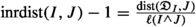
We define the inner relative distance of J and I by

$$\begin{aligned} \mathrm{\, inrdist}(I,J)= 1+\frac{\textrm{dist}(J,{\mathfrak {D}}_{I})}{\ell (J)}. \end{aligned}$$

This quantity is comparable to $\max (1,j)$, where j is the smallest number of times J needs to be shifted a distance equal to its side length so that the translated cube intersects ${\mathfrak {D}}_{I}$.

Definition 4.1

For every $M\in {\mathbb {N}}$, let ${{\mathcal {C}}}_{M}$ be the family of cubes in ${\mathbb {R}}^{n}$ such that $2^{-M}\le \ell (I)\le 2^{M}$ and $\mathrm{\, rdist}(I,{\mathbb {B}}_{2^{M}})\le M$. We define ${\mathcal D}_{M}={{\mathcal {D}}}\cap {{\mathcal {C}}}_{M}$ and ${{\mathcal {D}}}_{M}(\Omega )={{\mathcal {D}}}(\Omega )\cap {{\mathcal {C}}}_{M}$.

For any given $M\ge 0$, we call the cubes in ${{\mathcal {C}}}_{M}$ and ${{\mathcal {D}}}_{M}$ as lagom cubes and dyadic lagom cubes respectively.

4.2 Conditions for Membership to the Schatten Classes

We state in this section the functions whose summability implies membership of the operators under study to the Schatten classes.

Let $\delta >0$ and $L,S, D: [0,\infty )\rightarrow [0,\infty )$ satisfying

$$\begin{aligned} \lim _{x\rightarrow \infty }L(x) =\lim _{x\rightarrow 0}S(x) =\lim _{x\rightarrow \infty }D(x)=0. \end{aligned}$$

(5)

With loss of generality, we assume that L and D are non-decreasing, and S is non-increasing.

For fixed $0<\theta <1$, we denote the corresponding dilated functions as

$$\begin{aligned} {\tilde{L}} (x)&=\sup _{0<\lambda \le 1}\lambda ^{\frac{\delta }{1+2\delta }\theta }L(\lambda x), \hspace{50.0pt}{\tilde{D}} (x)=\sup _{0<\lambda \le 1} \lambda ^{\frac{d}{2}\theta }D(\lambda x). \end{aligned}$$

By Lebesgue’s Dominated Convergence Theorem, the functions $\tilde{L}$ and ${{\tilde{D}}}$ also satisfy (5). Given three cubes $I_{1},I_{2},I_{3}$, we define

$$\begin{aligned} F_K(I_{1}, I_{2}, I_{3})= & {} L(\ell (I_{1}))S(\ell (I_{2}))D(\mathrm{\, rdist}(I_{3},{\mathbb {B}}))\\ {{\tilde{F}}}_K(I_{1}, I_{2}, I_{3})= & {} {{\tilde{L}}} (\ell (I_{1}))S(\ell (I_{2})){{\tilde{D}}} (\mathrm{\, rdist}(I_{3},{\mathbb {B}})), \end{aligned}$$

and the corresponding $F_K(I)=F_K(I,I,I)$, ${{\tilde{F}}}_K(I)=\tilde{F}_K(I,I,I)$.

Let $F_K(t,x)$ as in (2), $F_W(I)$ as in (4), and the dilation just defined $\tilde{F}_K(I)$. We define for $0<p\le 2$,

$$\begin{aligned} F_s(I)={{\tilde{F}}}_K(I)+F_W(I)+\textrm{osc}_{I}(T1)+\textrm{osc}_{I}(T^{*}1). \end{aligned}$$

(6)

On the other hand, for $2<p\le \infty$, given L, S, D as before and $0<\delta '<\delta$, we define

• $L^{\theta }(x) =L(x)+L(x^{1-\theta })+L(x^{1+(1-\theta )/{\delta '}}) +(1+x^{\theta \delta '})^{-1} +x^{1-\theta }\mathbb {1}_{[0,1]}(x)$

• $S^{\theta }(x) =S(x)+S(x^{1-\theta }) +\frac{x^{\theta \delta '}}{1+x^{\theta \delta '}}$

• $D^{\theta }(x) =D(x)+D(x^{1-\theta }) +(1+x^{\theta \delta '})^{-1}.$

Now, given these three new functions, we define the corresponding ${{\tilde{F}}}_K^{\theta }$ in a similar way we did before. Then we define

$$\begin{aligned} F_l(I)={{\tilde{F}}}_K^{\theta }(I)+F_W(I)+\textrm{osc}_{I}(T1)+\textrm{osc}_{I}(T^{*}1). \end{aligned}$$

(7)

With these definitions, we can state our main result.

Theorem 4.2

Let T be a linear operator with a compact Calderón–Zygmund kernel K and associated function F defined in (6).

• (1) If $0<p\le 2$ and $\displaystyle {\sum _{I\in {\mathcal {D}}} F_s(I)^p<\infty }$, then $T\in S_{p}(L^{2}({\mathbb {R}}^{d}))$.

• (2) If $2<p$ and $\displaystyle {\sum _{I\in {\mathcal {D}}} F_l (I)^p<\infty }$, then $T\in S_{p}(L^{2}({\mathbb {R}}^{d}))$.

Remark 4.3

Each of these two conditions implies $T1, T^*1\in \textrm{SMO}_p$.

5 Characterization of the Schatten Classes by Means of Frames of $L^2({\mathbb {R}}^d)$

5.1 Frames on Hilbert Spaces

Operators in the Schatten classes can be characterized by their action on frames.

Definition 5.1

Let H be a separable Hilbert space. A sequence of functions $(f_n)_{n\in {\mathbb {N}}}\subset H$ is a frame for H if there exist constants $0<C_1\le C_2$ such that

$$\begin{aligned} C_1\Vert f\Vert ^2\le \sum _{n\in {\mathbb {N}}} |\langle f,f_n\rangle |^2 \le C_2\Vert f\Vert ^2 \end{aligned}$$

for all $f\in H$.

For a given frame $(f_n)_{n\in {\mathbb {N}}}$, the largest possible constant $C_1$ in previous inequality is called the lower frame bound, while the smallest possible constant $C_2$ is called the upper frame bound.

A frame is called normalized tight if its lower and upper frame bounds are both equal to 1.

The notion of frame was first introduced by Duffin and Schaeffer [15]. Since then it has found a multitude of applications both in fundamental and applied analysis. The literature on frames, most notably Gabor and wavelet frames, is truly vast. See [8, 9, 19, 22] and [7] for a very small sample.

There are several characterizations of the Schatten classes in terms of orthogonal bases and frames. We use the following results, which are contained in [3]. It should be noted that the statements in the referenced paper are written in a slightly different way.

Theorem 5.2

Let T be a bounded operator on a separable Hilbert space H and $0<p\le 2$. Then $T\in S_{p}$ if and only if there is at least one frame $(f_{n})_{n\in {\mathbb {N}}}$ of H such that

$$\begin{aligned} \sum _{n\in {\mathbb {N}}} \Vert Tf_{n}\Vert ^{p}<\infty . \end{aligned}$$

Moreover,

$$\begin{aligned} \Vert T\Vert _{p}=\inf \left( \sum _{n\in {\mathbb {N}}} \Vert f_{n}\Vert ^{2-p} \Vert Tf_{n}\Vert ^{p}\right) ^{\frac{1}{p}}, \end{aligned}$$

(8)

where the infimum is calculated over all frames $(f_{n})_{n\in {\mathbb {N}}}$ of H with lower frame bound larger or equal to 1.

Theorem 5.3

Let T be a compact operator on a separable Hilbert space H and $2< p\le \infty$. Then $T\in S_{p}$ if and only if there exists $C>0$ such that

$$\begin{aligned} \sum _{n\in {\mathbb {N}}} \Vert Tf_{n}\Vert ^{p}\le C \end{aligned}$$

for every frame $(f_{n})_{n\in {\mathbb {N}}}$ of H. Moreover,

$$\begin{aligned} \Vert T\Vert _{p}=\sup \left( \sum _{n\in {\mathbb {N}}} \Vert Tf_{n}\Vert ^{p}\right) ^{\frac{1}{p}}, \end{aligned}$$

where the supremum is calculated over all frames $(f_{n})_{n\in {\mathbb {N}}}$ of H with upper frame bound smaller or equal to 1.

For small exponents we use Theorem 5.2. However, for large exponents we cannot directly use Theorem 5.3 because we do not have control of the action of a Calderón–Zygmund operator over all possible frames (not even on all orthonormal bases). Instead, we will resort to the following property of the Schatten classes whose proof when $n=0$ is classical (see [38]).

Theorem 5.4

Let T be a compact operator on H, $p>0$ and $n\ge 0$. Then $T\in S_p$ if and only if $(T^*T)^{2^n}\in S_{p/2^{n+1}}$. Moreover, $\Vert T\Vert _p= \Vert (T^*T)^{2^n}\Vert _{\frac{p}{2^{n+1}}}^{\frac{1}{2^{n+1}}}$.

Proof

By definition, the singular values $s_n$ of T are the square roots of the eigenvalues $\lambda _n$ of $T^*T$, that is, $s_n=\lambda _n^{1/2}$.

Since $T^*T$ is self-adjoint and positive, its singular values are exactly its eigenvalues $\lambda _n$. Then

$$\begin{aligned} \Vert T\Vert _p^p=\sum _n s_n^p=\sum _n\lambda _n^{\frac{p}{2}} =\Vert T^*T\Vert _{\frac{p}{2}}^{\frac{p}{2}} \end{aligned}$$

By a reiteration of previous argument, we get that $T\in S_p$ if and only if $T^*T\in S_{\frac{p}{2}}$ if and only if $(T^*T)^2=(T^*T)^*T^*T\in S_{\frac{p}{4}}$ if and only if $(T^*T)^{2^n}\in S_{\frac{p}{2^{n+1}}}$. In each case we have

$$\begin{aligned} \Vert T\Vert _p= \Vert T^*T\Vert _{\frac{p}{2}}^{\frac{1}{2}} =\Vert (T^*T)^2\Vert _{\frac{p}{4}}^{\frac{1}{4}} =\cdots = \Vert (T^*T)^{2^n}\Vert _{\frac{p}{2^{n+1}}}^{\frac{1}{2^{n+1}}}. \end{aligned}$$

$\square$

5.2 A Haar-Type Wavelet Frame

Definition 5.5

For each a dyadic cube $I\in {\mathcal {D}}$, we define the corresponding Haar wavelet as

$$\begin{aligned} \psi _{I}=|I|^{-\frac{1}{2}}\big (\mathbb {1}_{I} -2^{-d}\mathbb {1}_{{\widehat{I}}}\big ), \end{aligned}$$

where $I\in \textrm{ch}({\widehat{I}})$, that is, $I\subset {\widehat{I}}$ such that $\ell (I)=\ell ({\widehat{I}})/2$.

We denote $\langle f,g\rangle =\int _{{\mathbb {R}}^{d}}f(x)g(x)dx$. We hope that this non-stardard use of the notation $\langle ,\rangle$ which is quite customary in the literature on Tb theorems will not cause any confusion.

The following result summarizes the orthogonality properties of the Haar wavelet frame. The proof follows directly by using Definition 5.5.

Lemma 5.6

Let $I,J\in {\mathcal {D}}$. Then

$$\begin{aligned} \langle \psi _I,\psi _J\rangle =\delta ({\widehat{I}},{\widehat{J}})(\delta (I,J)-2^{-d}), \end{aligned}$$

(9)

where $\delta (I,J)=1$ if $I=J$ and zero otherwise. With this we have $\Vert \psi _I\Vert _2=(1-2^{-d})^{\frac{1}{2}}$.

Lemma 5.7

The following decomposition

$$\begin{aligned} f=\sum _{I\in {\mathcal {D}}}\langle f, \psi _I\rangle \psi _I \end{aligned}$$

holds with convergence in $L^2({\mathbb {R}}^d)$. Moreover, $(\psi _I)_{I\in {{\mathcal {D}}}}$ is a normalized tight frame of $L^2({\mathbb {R}}^{d})$.

Proof

Let $f\in L^2({\mathbb {R}}^d)$. We start by noting that

$$\begin{aligned} \sum _{I\in \textrm{ch}({\widehat{I}})}\langle f, \psi _I\rangle \psi _I&=\sum _{I\in \textrm{ch}({\widehat{I}})}\langle f\rangle _I \mathbb {1}_{I} -2^{-d}\langle f\rangle _I \mathbb {1}_{{\widehat{I}}} -\langle f\rangle _{{\widehat{I}}}\mathbb {1}_{I} +2^{-d}\langle f\rangle _{{\widehat{I}}}\mathbb {1}_{{\widehat{I}}}\\&=\left( \sum _{I\in \textrm{ch}({\widehat{I}})}\langle f\rangle _I \mathbb {1}_I\right) - \langle f\rangle _{{\widehat{I}}}\mathbb {1}_{{\widehat{I}}}. \end{aligned}$$

Then, by summing a telescoping series, we get for all $x\in \mathbb R^d$

$$\begin{aligned} \sum _{\begin{array}{c} I\in {\mathcal {D}}\\ 2^{-N}\le \ell (I)< 2^N \end{array}}\langle f, \psi _I\rangle \psi _I (x)&=\sum _{\begin{array}{c} I\in {\mathcal {D}}\\ 2^{-N}\le \ell (I)< 2^N \end{array}}\left( \sum _{J\in \textrm{ch}(I)} \langle f\rangle _J \mathbb {1}_J(x)\right) - \langle f\rangle _{I}\mathbb {1}_{I}(x)\\&=\langle f\rangle _R \mathbb {1}_R(x)- \langle f\rangle _{S}\mathbb {1}_{S}(x), \end{aligned}$$

where R and S are the only dyadic cubes such that $\ell (R)=2^{-N}$, $\ell (S)=2^{N}$ and $x\in R\subset S$. Now, by Lebesgue’s Differentiation Theorem, the first term tends to f(x) almost everywhere when N tends to infinity. Meanwhile the second term tends to zero when N tends to infinity since $|\langle f\rangle _{S}|\le |S|^{-\frac{1}{2}}\Vert f\Vert _2=2^{-\frac{dN}{2}}\Vert f\Vert _2$. This proves a.e.-pointwise convergence.

Furthermore, if we denote by Mf the Hardy-Littlewood maximal function

$$\begin{aligned} Mf(x)=\sup _{\begin{array}{c} I\in {\mathcal {C}}\\ x\in I \end{array}}\frac{1}{|I|}\int _{I}f(y)dy, \end{aligned}$$

we have by previous calculations

$$\begin{aligned} |f(x)-\hspace{-.5cm} \sum _{\begin{array}{c} I\in {\mathcal {D}}\\ 2^{-N}\le \ell (I)< 2^N \end{array}}\hspace{-.2cm} \langle f, \psi _I\rangle \psi _I(x) |^2&\le (|f(x)|+\langle |f|\rangle _R \mathbb {1}_R(x)+ \langle |f|\rangle _{S}\mathbb {1}_{S}(x))^2\\&\lesssim |f(x)|^2+M(|f|)(x)^2, \end{aligned}$$

and the last function is integrable since $f, M(|f|)\in L^2$. Then by the a.e. pointwise convergence and Lebesgue’s Dominated Convergence Theorem, we obtain convergence on $L^2$.

Finally, to prove that $(\psi _I)_{I\in {{\mathcal {D}}}}$ is a normalized tight frame of $L^2({\mathbb {R}}^{d})$ we start by noting that norm convergence implies weak convergence, that is, for all $g\in L^2$

$$\begin{aligned} \lim _{N\rightarrow \infty }\int \sum _{\begin{array}{c} I\in {\mathcal {D}}\\ 2^{-N}\le \ell (I)< 2^N \end{array}}\langle f, \psi _I\rangle \psi _I (x)g(x)dx = \int f(x)g(x)dx. \end{aligned}$$

Then, by previous equality with $g=f$, we get

$$\begin{aligned} \Vert f\Vert _{2}^2&=\int _{{\mathbb {R}}^n}f(x)f(x)dx =\lim _{N\rightarrow \infty }\int f(x) \sum _{\begin{array}{c} I\in {\mathcal {D}}\\ 2^{-N}\le \ell (I)\le 2^{N} \end{array}} \langle f, \psi _{I}\rangle \psi _{I}(x)dx\\&=\lim _{N\rightarrow \infty }\sum _{\begin{array}{c} I\in {\mathcal {D}}\\ 2^{-N}\le \ell (I)\le 2^{N} \end{array}} \langle f, \psi _{I}\rangle \langle f, \psi _{I}\rangle =\sum _{I\in {\mathcal {D}}} |\langle f, \psi _{I}\rangle |^2, \end{aligned}$$

which ends the proof. $\square$

6 Bump Estimates for Compact Calderón–Zygmund Operators

Theorem 6.1 below, whose proof can be found in [36], describes the bump estimates satisfied by operators with a compact Calderón–Zygmund kernel for which special cancellations properties hold.

Proposition 6.1

Let T be a linear operator with a compact Calderón–Zygmund kernel with parameter $0<\delta <1$. We assume that T satisfies the weak compactness condition and $T1=T^{*}1=0$. Let $I, J\in {\mathcal {D}}$.

• (1) When $\mathrm{\, rdist}(\,{\widehat{I}},{\widehat{J}}\,)> 3$,

  $$\begin{aligned} |\langle T\psi _{I},\psi _{J}\rangle | \lesssim \frac{\textrm{ec}(I,J)^{\frac{d}{2}+\delta }}{\mathrm{\, rdist}(I,J)^{d+\delta }} F_1(I,J), \end{aligned}$$

  where . Alternatively, we also have

  $$\begin{aligned} |\langle T\psi _{I},\psi _{J}\rangle | \lesssim \frac{\textrm{ec}(I,J)^{-\frac{d}{2}}}{\mathrm{\, inrdist}(I,J)^{d+\delta }} F_1(I,J). \end{aligned}$$

• (2) When $\mathrm{\, rdist}(\,{\widehat{I}},{\widehat{J}}\,)\le 3$,

  $$\begin{aligned} |\langle T\psi _{I},\psi _{J}\rangle |&\lesssim \frac{\textrm{ec}(I,J)^{\frac{d}{2}}}{\mathrm{\, inrdist}(I,J)^{\delta }} F_{2}(I, J), \end{aligned}$$

  where , with $\delta (I,J)=1$ if $I=J$ and zero otherwise.

7 The Schatten Classes for Small Exponents

We now start the proof of Theorem 4.2, our main result on singular integral operators in the Schatten class. We distinguish between exponents smaller than two, which we treat in this section, and larger than 2, which is dealt in Sect. 9 with preliminary work in Sect. 8.

In each case we work first the special cancellation case, that is, when $T1=T^*1=0$, and treat later the general case of $T1,T^*1\in \textrm{SMO}_p$ by means of paraproducts.

7.1 Proof of Theorem 4.2 Under Special Cancellation Conditions and $0<p\le 2$

Theorem 7.1

Let T be a linear operator with a compact Calderón–Zygmund kernel and associated function $F_s$ as defined in (6). We assume that $T1=T^*1=0$. Let $0<p\le 2$.

If $\displaystyle {\sum _{I\in {\mathcal {D}}} F_s(I)^p<\infty }$, then T belongs to the Schatten class $S_{p}(L^{2}({\mathbb {R}}^{d}))$.

Proof

Let $(\psi _{I})_{I\in {{\mathcal {D}}}}$ be the Haar wavelet frame of $L^{2}({\mathbb {R}}^{d})$ given in Definition 5.5. By Theorem 5.2, to prove membership of T on the Schatten class $S_{p}$ we just need to show $\sum _{I\in {\mathcal D}}\Vert T\psi _{I}\Vert _{2}^{p}<\infty .$ Once we show that

$$\begin{aligned} \Vert T\psi _{I}\Vert _{2} \lesssim F_s(I) \end{aligned}$$

(10)

we have

$$\begin{aligned} \sum _{I\in {{\mathcal {D}}}}\Vert T\psi _{I}\Vert _{2}^{p} \lesssim \sum _{I\in {{\mathcal {D}}}}F_s(I)^{p}, \end{aligned}$$

which is finite by hypothesis. To prove (10) we start by writing

$$\begin{aligned} \Vert T\psi _{I}\Vert _{2} \lesssim \left( \sum _{J\in {{\mathcal {D}}}}|\langle T\psi _{I},\psi _{J}\rangle |^{2}\right) ^{\frac{1}{2}}. \end{aligned}$$

In view of the rate of decay stated in the bump estimates of Proposition 6.1, we parametrize the sums accordingly with the eccentricity, relative distance, and inner relative distance of the cubes I, J as follows. For fixed $e\in {\mathbb {Z}}$, $m\in {\mathbb {N}}$ and every dyadic cube J, we define the families

$$\begin{aligned} I_{e,m}=I_{e,m,0}=\{ J\in {{\mathcal {D}}}:\ell (I)=2^{e}\ell (J), m\le \mathrm{\, rdist}(I,J)< m+1 \}, \end{aligned}$$

and when $m\le 3$

$$\begin{aligned} I_{e,m,k}=\{ J\in I_{e,m}: k\le \mathrm{\, inrdist}(I,J)<k+1\}. \end{aligned}$$

We note that the cardinality of $I_{e,m}$ is comparable to $2^{\max (e,0)n}m^{d-1}$, while the cardinality of the family $I_{e,m,k}$ is bounded by a constant times $2^{\max (e,0)(d-1)\frac{\max (e,0)}{e}}$. Then we have

$$\begin{aligned} \Vert T\psi _{I}\Vert _{2} \lesssim \left( \sum _{e\in {\mathbb {Z}}}\sum _{m,k\in {\mathbb {N}}} \sum _{J\in I_{e,m,k}}| \langle T\psi _{I},\psi _{J}\rangle |^{2}\right) ^{\frac{1}{2}}. \end{aligned}$$

By Proposition 6.1, we have for $m>3$,

$$\begin{aligned} |\langle T\psi _I,\psi _J\rangle | \lesssim 2^{-|e|(\frac{d}{2}+\delta )}m^{-(d+\delta )} F(I,J), \end{aligned}$$

while when $m\le 3$,

$$\begin{aligned} |\langle T\psi _I,\psi _J\rangle | \lesssim 2^{-|e|\frac{d}{2}}k^{-\delta } F(I,J), \end{aligned}$$

with or . We write both estimates in a unified manner as

$$\begin{aligned} |\langle T\psi _I,\psi _J\rangle | \lesssim A_{e,m,k} F(I,J). \end{aligned}$$

With this

$$\begin{aligned} \Vert T\psi _{I}\Vert _{2} \lesssim \left( \sum _{e\in {\mathbb {Z}}}\sum _{m,k\in {\mathbb {N}}}A_{e,m,k}^{2} \sum _{J\in I_{e,m,k}} F(I,J)^{2}\right) ^{\frac{1}{2}}. \end{aligned}$$

(11)

a) For $m>3$, we have

We first show that when $J\in I_{e,m}$, we have

$$\begin{aligned} F(I,J)&\lesssim L(\ell (I))S(\ell (I))D(\lambda _{e,m}\mathrm{\, rdist}(I,{\mathbb {B}}))= F_{e,m}(I). \end{aligned}$$

(12)

where $\lambda _{e,m}=2^{\min (e,0)}m^{-1}\le 1$.

For this, we remind that L is non-increasing and S is non-decreasing. Since , and , we have $L(\ell (\langle I,J\rangle )) \le L(\ell (I))$ and . This enough to control L and S.

On the other hand, since D is non-increasing, we work to prove the lower bound

$$\begin{aligned} \mathrm{\, rdist}(\langle I,J\rangle ,{\mathbb {B}}) > rsim \lambda _{e,m}\mathrm{\, rdist}(I ,{\mathbb {B}}) . \end{aligned}$$

We first we note that since $\mathrm{\, rdist}(I,J)\le m+1\le 2m$, we have . Then for $e\ge 0$ we have $\ell (\langle I,J\rangle )\lesssim m\ell (I)$, while for $e\le 0$ we get $\ell (\langle I,J\rangle )\lesssim m\ell (J)=m2^{-e}\ell (I)$. That is, $\ell (\langle I,J\rangle )\lesssim m2^{-\min (e,0)}\ell (I)=\lambda _{e,m}^{-1}\ell (I)$. With this $1+\ell (\langle I,J\rangle )\lesssim \lambda _{e,m}^{-1}(1+\ell (I))$.

Moreover, since $c(I)\in \langle I,J\rangle$ we have $|c(\langle I,J\rangle )-c(I)|\le \ell (\langle I,J\rangle )/2$. Then

$$\begin{aligned} \mathrm{\, rdist}(\langle I,J\rangle ,{\mathbb {B}})& > rsim \frac{\ell (\langle I,J\rangle )+|c(\langle I,J\rangle )|+1}{1+\ell (\langle I,J\rangle )}\\& > rsim 1+\frac{|c(I)|}{1+\ell (\langle I,J\rangle )}\\& > rsim 1+\frac{|c(I)|}{\lambda _{e,m}^{-1}(1+\ell (I))}\\&\ge \frac{1}{\lambda _{e,m}^{-1}}\Big (1+\frac{|c(I)|}{1+\ell (I)}\Big )\\&\ge \lambda _{e,m}\mathrm{\, rdist}(I ,{\mathbb {B}}). \end{aligned}$$

Since D is non-increasing, we then have that $D(\mathrm{\, rdist}(\langle I,J\rangle ,{\mathbb {B}}))\lesssim D(\lambda _{e,m}\mathrm{\, rdist}(I,\mathbb B))$. With the three inequalities, we have

$$\begin{aligned} F(I,J)&\lesssim L(\ell (I))S(\ell (I))D(\lambda _{e,m}\mathrm{\, rdist}(I,{\mathbb {B}}))= F_{e,m}(I), \end{aligned}$$

as claimed in (12).

Now, using $A_{e,m,k}=2^{-|e|(\frac{d}{2}+\delta )}m^{-(d+\delta )}$, $\textrm{card}(I_{e,m})\approx 2^{\max (e,0)d}m^{d-1}$ and that $2^{\max (e,0)}2^{-\min (e,0)}=2^{|e|}$, we bound the corresponding terms in (11) by

$$\begin{aligned}&\left( \sum _{e\in {\mathbb {Z}}}\sum _{m>3}2^{-|e|(\frac{d}{2}+\delta )2}m^{-(d+\delta )2} \sum _{J\in I_{e,m}} F(I,J)^{2}\right) ^{\frac{1}{2}}\\&\quad \lesssim \left( \sum _{e\in \mathbb Z}\sum _{m>3}2^{-|e|(d+2\delta )}m^{-2(d+\delta )} 2^{\max (e,0)d}m^{d-1} F_{e,m}(I)^{2}\right) ^{\frac{1}{2}}\\&\quad = \left( \sum _{e\in {\mathbb {Z}}}\sum _{m>3}2^{-|e|2\delta } m^{-(1+2\delta )}2^{\min (e,0)d}m^{-d} F_{e,m}(I)^{2}\right) ^{\frac{1}{2}}\\&\quad = \left( \sum _{e\in {\mathbb {Z}}}\sum _{m>3}2^{-|e|2\delta } m^{-(1+2\delta )}\lambda _{e,m}^d F_{e,m}(I)^{2}\right) ^{\frac{1}{2}}\\&\quad \le \sup _{e\in {\mathbb {Z}}, m>3} \lambda _{e,m}^{\frac{d}{2}} F_{e,m}(I) \left( \sum _{e\in {\mathbb {Z}}}\sum _{m>3}2^{-|e|2\delta } m^{-(1+2\delta )}\right) ^{\frac{1}{2}}\\&\quad \lesssim F_s(I). \end{aligned}$$

The last inequality is due to the fact that

$$\begin{aligned} \sup _{e\in {\mathbb {Z}}, m>3} \lambda _{e,m}^{\frac{d}{2}} F_{e,m}(I)&=L(\ell (I))S(\ell (I))\sup _{0<\lambda \le 1} \lambda ^{\frac{d}{2}} D(\lambda I)\\&=L(\ell (I))S(\ell (I)){{\tilde{D}}}(I) ={{\tilde{F}}}_{K}(I)\le F_s(I) \end{aligned}$$

as defined in (6) at Definition 4.1. This shows that the terms corresponding to this case satisfy (10).

b) Now we deal with the case $1\le m\le 3$, for which we have

We show that $1\le k\lesssim 2^{\max (e,0)}$: since

we have . Then

which proves the inequality.

As before, we are going to estimate F(I, J) when $J\in I_{e, m,k}$. Then, given $I\in {\mathcal {D}}$, we denote

$$\begin{aligned} F_{e}(I)=\sup _{\begin{array}{c} 1\le m\le 3\\ 1\le k\le 2^{\max (e,0)} \end{array}}\sup _{J\in I_{e,m,k}}F(I,J). \end{aligned}$$

We also denote $M(e)=\max (e,0)$ and $m(e)=\min (e,0)$. Then we use $A_{e,m,k}=2^{-|e|\frac{d}{2}}k^{-\delta }$, and $\textrm{card}(I_{e,m,k})\lesssim 2^{M(e)(d-1) }$ to show that the corresponding terms in (11) can be bounded by

$$\begin{aligned}&\left( \sum _{e\in \mathbb Z}\sum _{k=1}^{2^{M(e)}}2^{-|e|d}k^{-2\delta } \sum _{J\in I_{e,m,k}} F(I,J)^{2}\right) ^{\frac{1}{2}}\\&\quad \le \left( \sum _{e\in \mathbb Z}\sum _{k=1}^{2^{M(e)}}2^{-|e|d}k^{-2\delta } 2^{M(e)(d-1) } F_{e}(I)^{2}\right) ^{\frac{1}{2}}\\&\quad \le \left( \sum _{e\in {\mathbb {Z}}}2^{-|e|d^{\alpha }} F_{e}(I)^{2}\sum _{k=1}^{2^{M(e)}}k^{-2\delta } \right) ^{\frac{1}{2}}, \end{aligned}$$

since $2^{-|e|d}2^{M(e)(d-1) } =2^{-|e|d^{\alpha }}$ with $\alpha =\frac{m(e)}{e}$. Now let $\theta =\frac{1}{2\delta +1}$, which satisfies $0<\theta <1$. Then

$$\begin{aligned} \sum _{k=1}^{2^{M(e)}} k^{-2\delta }&= \sum _{k=1}^{2^{\theta M(e)}} k^{-2\delta } +\sum _{k=2^{\theta M(e)}+1}^{2^{M(e)}} k^{-2\delta }\\&\lesssim 2^{\theta M(e)} +2^{-2\delta \theta M(e) }2^{M(e)} \lesssim 2^{M(e)\frac{1}{2\delta +1}}. \end{aligned}$$

With this, the corresponding terms in (11) can be bounded by

$$\begin{aligned} \left( \sum _{e\in {\mathbb {Z}}}2^{-|e|d^{\alpha }+M(e)\frac{1}{2\delta +1}}F_{e}(I)^{2} \right) ^{\frac{1}{2}}. \end{aligned}$$

We note that $-|e|d^{\alpha }+M(e)\frac{1}{2\delta +1}=-|e|\beta$ such that if $e\ge 0$ then $\beta =1-\frac{1}{2\delta +1}=\frac{2\delta }{1+2\delta }$, while if $e\le 0$, then $\beta =d$. With this, and the inequalities $0<\alpha$, $0<\theta <1$, we can bound previous expression by

$$\begin{aligned}&\sup _{e\in {\mathbb {Z}}}2^{-|e|\frac{\beta }{2}\theta }F_{e}(I) \Big ( \sum _{e\in {\mathbb {Z}}} 2^{-|e|\beta (1-\theta )} \Big )^{\frac{1}{2}} \lesssim \sup _{e\in {\mathbb {Z}}}2^{-|e|\frac{\beta }{2}\theta }F_{e}(I). \end{aligned}$$

From now we work to show that $2^{-|e|\frac{\beta }{2}\theta }F_{e}(I)\lesssim {{\tilde{F}}}(I)$. We start dealing with the first term:

(13)

Since , we immediately have . For the factor given by D, we first note that by the work carried out in the previous case and $m\le 3$ we have

$$\begin{aligned} \mathrm{\, rdist}(\langle I,J\rangle ,{\mathbb {B}}) > rsim \frac{2^{\min (e,0)}}{m}\mathrm{\, rdist}(I ,{\mathbb {B}}) > rsim 2^{\min (e,0)}\mathrm{\, rdist}(I ,{\mathbb {B}}). \end{aligned}$$

Then we can bound (13) by

To deal with L we reason as follows. When $\ell (I)\le \ell (J)$, we have $e\le 0$ and . Then previous expression equals

$$\begin{aligned} L(\ell (I))S(\ell (I))D(2^{e}\mathrm{\, rdist}(I,{\mathbb {B}})) \end{aligned}$$

and thus

$$\begin{aligned} \sup _{\begin{array}{c} e\in {\mathbb {Z}}\\ e\le 0 \end{array}}2^{-|e|\frac{\beta }{2}\theta }F_{e}(I)&\lesssim L(\ell (I)S(\ell (I))2^{e\frac{d}{2}\theta }D(2^{e}\mathrm{\, rdist}(I ,\mathbb B))\\&\le L(\ell (I)S(\ell (I)){{\tilde{D}}}(\mathrm{\, rdist}(I ,{\mathbb {B}})) \le F_s(I). \end{aligned}$$

On the other hand, when $\ell (J)\le \ell (I)$, we have with $e\ge 0$. Then $\beta =\frac{\delta }{1+2\delta }$ and

$$\begin{aligned} \sup _{\begin{array}{c} e\in {\mathbb {Z}}\\ e\ge 0 \end{array}}2^{-|e|\frac{\beta }{2}\theta }F_{e}(I)&\lesssim \sup _{e\in {\mathbb {Z}}} 2^{-e\frac{\delta }{1+2\delta }\theta } L(2^{-e}\ell (I))S(\ell (I)) D(\mathrm{\, rdist}(I,{\mathbb {B}}))\nonumber \\&\le {\tilde{L}}(\ell (I))S(\ell (I)) D(\mathrm{\, rdist}(I,{\mathbb {B}}))\le F_s(I). \end{aligned}$$

(14)

Finally, by definition we have that $F_W(I)\le {{\tilde{F}}}(I)$. This completely finishes the proof of (10). $\square$

7.2 Proof of Theorem 4.2 in the General Case. Compact Paraproducts

When T1, $T^{*}1$ are arbitrary functions in $\textrm{SMO}_{p}(\mathbb R^{d})$, we construct paraproducts $\Pi _{T1}$, $\Pi _{T^{*}1}^{*}$ with compact Calderón–Zygmund kernels such that $\Pi _{T1}(1)=T1$, $\Pi _{T^{*}1}^{*}(1)=0$ while $\Pi _{T1}^{*}(1)=0$, $\Pi _{T^{*}1}(1)=T^{*}1$. This way, the operator

$$\begin{aligned} {\tilde{T}}=T-\Pi _{T1}-\Pi _{T^{*}1}^{*} \end{aligned}$$

satisfies the hypotheses of Theorem 7.1 and so, ${\tilde{T}}$ belongs to $S_{p}({\mathbb {R}}^{d})$. Then, to prove that the initial operator T is also in $S_{p}({\mathbb {R}}^{d})$, we just need to show that the paraproducts $\Pi _{T1}$ and $\Pi _{T^{*}1}^{*}$ are in $S_{p}({\mathbb {R}}^{d})$.

Definition 7.2

Let $(\psi _I)_{I\in {\mathcal {D}}}$ be the Haar wavelet system of Definition 5.5. Let b a locally integrable function. We define the linear operator

$$\begin{aligned} \langle \Pi _{b}f,g\rangle&=\sum _{I\in {\mathcal {D}}} \langle b, \psi _{I}\rangle \langle f\rangle _{I} \langle g,\psi _{I}\rangle \end{aligned}$$

(15)

for all $f,g\in {{\mathcal {C}}}_{0}({\mathbb {R}}^{d})$.

Notation 7.3

For $I,J\in {\mathcal {I}}$, we define $\delta _{J\subseteq I}=1$ if $J\subseteq I$ and zero otherwise.

Proposition 7.4

Let $T1\in \textrm{SMO}_{p}({\mathbb {R}}^{d})$ for $0< p\le 2$. Then both $\Pi _{T1}$ and $\Pi _{T1}^*$ can be associated with a compact Calderón–Zygmund kernel, and they belong to $S_{p}({\mathbb {R}}^{d})$ with $\Vert \Pi _{T1}\Vert _{S_p}\lesssim \Vert T1\Vert _{ \textrm{SMO}_{p}}$ and $\Vert \Pi _{T1}^*\Vert _{S_p}\lesssim \Vert T1\Vert _{ \textrm{SMO}_{p}}$. Moreover, $\langle \Pi _{T1}1,g\rangle =\langle T1,g\rangle$ and $\langle \Pi _{T1}^{*}1,f\rangle =0$.

Proof

The fact that both $\Pi _{T1}$ and $\Pi _{T1}^*$ both have a compact Calderón–Zygmund kernel was already proved in [35].

Formally, $\Pi _{T1}$ satisfies

$$\begin{aligned} \langle \Pi _{T1}1,g\rangle =\sum _{I\in {\mathcal {D}}}\langle T1, \psi _{I}\rangle \langle g, \psi _{I}\rangle =\langle T1, g\rangle . \end{aligned}$$

Moreover, since $\psi _I$ has mean zero, we have $\langle \Pi _{T1}f,1\rangle =0$.

Since $0<p\le 2$, to prove membership to $S_p$ we just need to show that $\sum _{I\in {\mathcal {D}}}\Vert \Pi _{T1}\psi _{I}\Vert _{2}^{p}$ is finite. As before, we start with

$$\begin{aligned} \Vert \Pi _{T1}\psi _{I}\Vert _{2}^{p} \lesssim \left( \sum _{J\in \mathcal D}|\langle \Pi _{T1}\psi _{I},\psi _{J}\rangle |^{2}\right) ^{\frac{p}{2}}. \end{aligned}$$

By definition of the paraproduct and the orthogonality property (9),

$$\begin{aligned} \langle \Pi _{T1}\psi _{I},\psi _{J}\rangle&=\sum _{K\in {\mathcal {D}}}\langle T1, \psi _{K}\rangle \langle \psi _I\rangle _K \langle \psi _K,\psi _J\rangle \\&=\sum _{K\in \textrm{ch}({\widehat{J}}\,)}\langle T1, \psi _{K}\rangle \langle \psi _{I}\rangle _{K}(\delta (J, K)-2^{-d}). \end{aligned}$$

Since $\psi _I$ is supported on ${\widehat{I}}$ and it has mean zero, we have that $\langle \psi _I\rangle _K =0$ unless $K\subsetneq {\widehat{I}}$. With this and $K\in \textrm{ch}({\widehat{J}})$ we get ${\widehat{J}}\subseteq {\widehat{I}}$ and so

$$\begin{aligned} \langle \Pi _{T1}\psi _{I},\psi _{J}\rangle&=\delta _{{\widehat{J}}\subseteq {\widehat{I}}}\sum _{K\in \textrm{ch}({\widehat{J}}\,)}\langle T1, \psi _{K}\rangle \langle \psi _{I}\rangle _{K}(\delta (J, K)-2^{-d}). \end{aligned}$$

(16)

Now, since $|\delta (K,J)-2^{-d}|\le 2$ and $|\langle \psi _{I}\rangle _K |\lesssim \frac{1}{|I|^{\frac{1}{2}}}$, we get

$$\begin{aligned} |\langle \Pi _{T1}\psi _{I},\psi _{J}\rangle |&\le 2\delta _{{\widehat{J}}\subseteq {\widehat{I}}} \, \frac{1}{|I|^{\frac{1}{2}}} \sum _{K\in \textrm{ch}({\widehat{J}})} |\langle T1, \psi _{K}\rangle |. \end{aligned}$$

(17)

Then

$$\begin{aligned} \Vert \Pi _{T1}\psi _{I}\Vert _{2}^{p}&\lesssim \left( \frac{1}{|I|}\sum _{\begin{array}{c} J\in {\mathcal {D}}\\ {\widehat{J}}\subseteq {\widehat{I}} \end{array}} \sum _{K\in \textrm{ch}({\widehat{J}})}|\langle T1, \psi _{K}\rangle |^{2}\right) ^{\frac{p}{2}}\\&\lesssim \left( \frac{1}{|I|}\sum _{\begin{array}{c} J\in {\mathcal {D}}\\ J\subsetneq {\widehat{I}} \end{array}} |\langle T1, \psi _{J}\rangle |^{2}\right) ^{\frac{p}{2}} \lesssim \textrm{osc}_{I}(T1)^p. \end{aligned}$$

Since $\Vert \psi _{I}\Vert _2=(1-2^{-d})^{\frac{1}{2}}\le 1$ and $p\le 2$, by (8) this finally shows

$$\begin{aligned} \Vert \Pi _{T1}\Vert _{S_p}^p&\le \sum _{I\in {\mathcal {D}}} \Vert \Pi _{T1}\psi _{I}\Vert _{2}^{p} \lesssim \sum _{I\in \mathcal D}\textrm{osc}_{{\widehat{I}}}(T1)^{p}\\&\lesssim \sum _{I\in {\mathcal {D}}}\textrm{osc}_I(T1)^{p} = \Vert T1\Vert _{\textrm{SMO}_p}^p. \end{aligned}$$

On the other hand, $\Vert \Pi _{T1}^*\Vert _p=\Vert \Pi _{T1}\Vert _p \lesssim \Vert T1\Vert _{\textrm{SMO}_p}$. $\square$

8 Technical Results

Theorem 6.1 shows the estimates satisfied by Calderón–Zygmund operators T that extend compactly on $L^p({\mathbb {R}}^d)$. In Theorem 9.1, we prove an extension of Theorem 6.1 satisfied by dyadic powers of $T^*T$.

Prior to the proof of Theorem 9.1, we need to develop nine technical lemmata that will be used in its demonstration. These results are classified in four groups, depending on the object being estimated: elementary integrals, convolutions, distances, and the function F.

8.1 Estimates on Elementary Integrals

We start with a lemma on estimates of some elementary integrals.

Lemma 8.1

Let $0<\delta <1$, $a\in {\mathbb {R}}^d$, $R\ge 0$ and $0\le R_1\le R_2$. Then

$$\begin{aligned} \int \limits _{B(0,R)}(1+|x-a|)^{-(d+\delta )}dx\lesssim & {} (1+\max (|a|-R,0))^{-\delta }, \end{aligned}$$

(18)

$$\begin{aligned} \int \limits _{B(0,R_2)\setminus B(0,R_1)}\hspace{-.5cm}(1+|x-a|)^{-(d+\delta )}dx\lesssim & {} \!(1+\max (|a|-R_2,R_1-|a|,0))^{-\delta }, \end{aligned}$$

(19)

$$\begin{aligned} \int \limits _{B(0,R)}(1+|x-a|)^{-\delta }dx\lesssim & {} (R+|a|)^{d-\delta }. \end{aligned}$$

(20)

Proof

A) We start by proving some related inequalities, (21) to (24), prior to demonstrate the inequalities in the statement.

1) To prove the new inequalities, we first assume $a=0$. Let $0<\theta \ne d$. Then

$$\begin{aligned}&\int \limits _{B(0,R_2)\setminus B(0,R_1)}(1+|x|)^{-\theta }dx \approx \int _{R_1}^{R_2}(1+r)^{-\theta }r^{d-1}dr\nonumber \\&\quad \approx \int \limits _{\min (\max (1,R_2),R_1)}^{\max (\min (1,R_2),R_1)}\hspace{-.2cm}r^{d-1}dr +\int \limits _{\max (\min (1,R_2),R_1)}^{R_2}\hspace{-.2cm}r^{d-1-\theta }dr\nonumber \\&\quad = d^{-1}(\max (\min (1,R_2),R_1)^{d}-\min (\max (1,R_2),R_1)^d)\nonumber \\&\quad \quad +(d-\theta )^{-1}(R_2^{d-\theta }-\max (\min (1,R_2),R_1)^{d-\theta })\nonumber \\&\quad \approx \max (\min (1,R_2),R_1)^{d} -\min (\max (1,R_2),R_1)^d\nonumber \\&\quad \quad +|R_2^{d-\theta }-\max (\min (1,R_2),R_1)^{d-\theta }|. \end{aligned}$$

(21)

Now we consider two cases in previous equivalence.

1.a) If $R_1=0$ and $R_2=R>1$, then from (21) we have

$$\begin{aligned} \int _{B(0,R)}(1+|x|)^{-\theta }dx&\lesssim \min (1,R)^{d}+|R^{d-\theta }-\min (1,R)^{d-\theta }|\\&\lesssim R^d\mathbb {1}_{[0,1]}(R) +(1+|R^{d-\theta }-1|)\mathbb {1}_{[1,\infty ]}(R)\\&\lesssim R^d\mathbb {1}_{[0,1]}(R)+(1+R)^{d-\theta }\mathbb {1}_{[1,\infty ]}(R). \end{aligned}$$

If $\theta =d+\delta$, we have

$$\begin{aligned} \int \limits _{B(0,R)}(1+|x|)^{-(d+\delta )}dx&\lesssim 1+(1+R)^{-\delta } \lesssim 1, \end{aligned}$$

(22)

while if $\theta =\delta < d$, we get

$$\begin{aligned} \int \limits _{B(0,R)}(1+|x|)^{-\delta }dx&\lesssim R^d\mathbb {1}_{[0,1]}(R) +R^{d-\delta }\mathbb {1}_{[1,\infty ]}(R) \lesssim R^{d-\delta }. \end{aligned}$$

(23)

1.b) On the other hand, if $R_1=R$ and $R_2=\infty$, and $\theta =d+\delta$ then from (21), we get

$$\begin{aligned} \int \limits _{{\mathbb {R}}^d\setminus B(0,R)}(1+|x|)^{-(d+\delta )}dx&\lesssim \max (1,R)^{d} -R^d +\max (1,R)^{-\delta }. \end{aligned}$$

If $R>1$, we have

$$\begin{aligned} \int \limits _{{\mathbb {R}}^d\setminus B(0,R)}(1+|x|)^{-(d+\delta )}dx&\lesssim \max (1,R)^{-\delta } \approx (1+R)^{-\delta }, \end{aligned}$$

while if $R\le 1$ we get

$$\begin{aligned} \int \limits _{{\mathbb {R}}^d\setminus B(0,R)}(1+|x|)^{-(d+\delta )}dx&\lesssim 1-R^d \lesssim 1\lesssim (1+R)^{-\delta }. \end{aligned}$$

With both things,

$$\begin{aligned} \int \limits _{{\mathbb {R}}^d\setminus B(0,R)}(1+|x|)^{-(d+\delta )}dx&\lesssim (1+R)^{-\delta }. \end{aligned}$$

(24)

2) Now for general $a\in {\mathbb {R}}^d$ we reason as follows. We first note that if $u_a=\frac{a}{|a|}$ is the unit vector in the direction of k, then

$$\begin{aligned} |Ru_a\pm a|^2&=R^2\pm 2\langle Ru_a,a\rangle +|a|^2 =R^2\pm 2\frac{R}{|a|}\langle a,a\rangle +|a|^2\\&=R^2\pm 2R|a|+|a|^2 =(R\pm |a|)^2 \end{aligned}$$

and so, $|Ru_a-a|=|R-|a||$ and $|Ru_a+a|=R+|a|$.

B) With all this preliminary work, we can now prove (18). We start by showing that if $R\le |a|$, then $B(-a,R)\subset {\mathbb {R}}^d\setminus B(0,|Ru_a-a|)$: for $x\in B(-a,R)$ we have $x=-a+Rv$ with $|v|\le 1$ and so

$$\begin{aligned} |x|&\ge |a|-R|v|\ge |a|-R=|Ru_a-a|. \end{aligned}$$

With this,

$$\begin{aligned} \int \limits _{B(0,R)}(1+|x-a|)^{-(d+\delta )}dx&=\int \limits _{B(-a,R)}(1+|x|)^{-(d+\delta )}dx\\&\lesssim \int \limits _{{\mathbb {R}}^d\setminus B(0,|Ru_a-a|)}(1+|x|)^{-(d+\delta )}dx\\&\lesssim (1+|Ru_a-a|)^{-\delta } =(1+||a|-R|)^{-\delta }, \end{aligned}$$

where we used (24) in the last inequality.

On the other hand, if $|a|\le R$, we have that $B(-a,R)\subset B(0,|a|+R)$. Then by (22)

$$\begin{aligned} \int \limits _{B(0,R)}(1+|x-a|)^{-(d+\delta )}dx&=\int \limits _{B(-a,R)}(1+|x|)^{-(d+\delta )}dx\\&\le \int \limits _{B(0,R+|a|)}(1+|x|)^{-(d+\delta )}dx \lesssim 1. \end{aligned}$$

Both inequalities prove (18).

C) To show (19) we reason as follows.

$$\begin{aligned} I&=\int \limits _{B(0,R_2)\setminus B(0,R_1)}(1+|x-a|)^{-(d+\delta )}dx\\&=\int \limits _{B(-a,R_2)\setminus B(-a,R_1)}(1+|x|)^{-(d+\delta )}dx . \end{aligned}$$

Let $C=B(-a,R_2)\setminus B(-a,R_1)$. If $R_2\le |a|$ then $C\subset {\mathbb {R}}^d\setminus B(0,|R_2u_a-a|)$. Meanwhile, if $|a|\le R_1$ then $C\subset {\mathbb {R}}^d\setminus B(0,|R_1u_a-a|)$. Therefore, by (24), we have in each case:

$$\begin{aligned} I&\lesssim (1+|R_2u_a-a|)^{-\delta } =(1+|a|-R_2)^{-\delta }, \end{aligned}$$

and

$$\begin{aligned} I&\lesssim (1+|R_1u_a-a|)^{-\delta } =(1+R_1-|a|)^{-\delta }, \end{aligned}$$

respectively. Meanwhile, if $R_1\le |a|\le R_2$, we have $B(-a,R_2)\setminus B(-a,R_1)\subset B(0,|a|+R_2)$ and so $I \lesssim 1.$ This ends the proof of (19).

D) To prove (20) we use that $B(-a,R)\subset B(0,|Ru_a+a|)$ and so

$$\begin{aligned} \int _{B(0,R)}(1+|x-a|)^{-\delta }dx&=\int \limits _{B(-a,R)}(1+|x|)^{-\delta }dx\\&\lesssim \int \limits _{{\mathbb {B}}(0,|Ru_a+a|)\setminus B(0,|Ru_a-a|)}(1+|x|)^{-\delta }dx\\&\lesssim |Ru_a+a|^{d-\delta }=(R+|a|)^{d-\delta }, \end{aligned}$$

where the last inequality follows from (23). This proves (20). $\square$

8.2 Estimates on Convolutions

The next two results consist on pointwise estimates for the convolution of integrable and non-integrable functions, Lemma 8.2 and Lemma 8.4 respectively.

Lemma 8.2

We denote $w(x)=(1+|x|)^{-(d+\delta )}$. For $m\in {\mathbb {Z}}^d$, and $\lambda \in {\mathbb {R}}$, we have

$$\begin{aligned} \sum _{m'\in {\mathbb {Z}}^d}w(\lambda m- m') w(m') \lesssim w(\lambda m), \end{aligned}$$

and

$$\begin{aligned} \sum _{m'\in {\mathbb {Z}}^d}w(m- \lambda m') w(m')&\lesssim \frac{w(m)}{1+(\frac{|\lambda | }{1+|m|})^d}\\&\quad +|\lambda |^{\delta } (1+\frac{1}{|\lambda |+|m|})^{\delta } w(|\lambda |+|m|). \end{aligned}$$

In both cases, the implicit constants are of the order of $\delta ^{-1}$.

Remark 8.3

We will mostly use the second inequality when $0<\lambda \le 1\le |m|$ and so, in that case the inequality simplifies to

$$\begin{aligned} \sum _{m'\in {\mathbb {Z}}^d}w(m- \lambda m') w(m')&\lesssim w(m). \end{aligned}$$

Proof

(1) When $\lambda m=0$, the first inequality holds trivially since we have $\sum _{m'\in {\mathbb {Z}}^d}w(m')^2 \lesssim 1$.

To prove the inequality when $\lambda m\ne 0$, we denote $c=\frac{\lambda m}{2}$, we consider the line $L=\langle \lambda m\rangle$, and the affine space of codimension one $H=c+L^\perp$ defined as the perpendicular complement of L translated to c. For $i\in \{0,1\}$, let $H_i$ be the d-dimensional sets defined by the closure of the connected components of ${\mathbb {R}}^d\setminus H$. Since $\lambda m\ne 0$, we can assume without loss of generality that $0\in H_0$ and $2c=\lambda m\in H_1$. Finally, we write $f(x)=w(x-\lambda m)$ and $g(x)=w(x)$. We also denote the left hand side of the first inequality by S. Then, by Hölder inequality,

$$\begin{aligned} S&= \sum _{m'\in {\mathbb {Z}}^d} f(m')g(m') \le \sum _{i=0,1}\sum _{m'\in H_i}f(m')g(m') \\&\le \Vert f\Vert _{l^\infty (H_0)}\Vert g\Vert _{l^1 (H_0)} +\Vert f\Vert _{l^1 (H_1)}\Vert g\Vert _{l^\infty (H_1)}. \end{aligned}$$

On $H_0$ we have $\Vert f\Vert _{l^\infty (H_0)} \le (1+|c-\lambda m|)^{-(d+\delta )} \lesssim (1+|\lambda m|)^{-(d+\delta )}=w(\lambda m)$, and $\Vert g\Vert _{l^1(H_0)}\le \Vert g\Vert _{l^1}\lesssim 1$, which accounts for the first term. On $H_1$ we have $\Vert g\Vert _{l^\infty (H_1)}\le (1+|c|)^{-(d+\delta )} \lesssim (1+|\lambda m|)^{-(d+\delta )}=w(\lambda m)$, and

$$\begin{aligned} \Vert f\Vert _{l^1(H_1)} \le \int _{{\mathbb {R}}^d} (1+|x-\lambda m|)^{-(d+\delta )}dx =\int _{{\mathbb {R}}^d} (1+|x|)^{-(d+\delta )}dx&\lesssim 1. \end{aligned}$$

This ends the proof of the first inequality.

(2) We denote again by S the left hand side of the second inequality. When $\lambda =0$, we have $S=\sum _{m'\in \mathbb Z^d}w(m)w(m') \lesssim w(m)$.

When $\lambda \ne 0$ and $m\ne 0$, we can assume by symmetry that $\lambda >0$. Then we apply previous reasoning to $c=\frac{\lambda ^{-1} m}{2}$, $H_0$, $H_1$ defined as before with $0\in H_0$, and $2c\in H_1$, $f(x)=w(\lambda x-m)$, and $g(x)=w(x)$. Then

$$\begin{aligned} S&\le \sum _{i=0,1}\sum _{m'\in H_i}f(m')g(m') \\&\le \min (\Vert f\Vert _{l^\infty (H_0)}\Vert g\Vert _{l^1 (H_0)}, \Vert f\Vert _{l^1 (H_0)}\Vert g\Vert _{l^\infty (H_0)}) \\&\quad +\min (\Vert f\Vert _{l^1 (H_1)}\Vert g\Vert _{l^\infty (H_1)}, \Vert f\Vert _{l^\infty (H_1)}\Vert g\Vert _{l^1 (H_1)}). \end{aligned}$$

On $H_0$, we have $\Vert f\Vert _{l^\infty (H_0)} \le (1+|\lambda c-m|)^{-(d+\delta )} \lesssim (1+|m|)^{-(d+\delta )}$ and $\Vert g\Vert _{l^1(H_0)}\lesssim 1$. On the other hand, we have that $H_0\subset {\mathbb {R}}^d\setminus B(\lambda ^{-1}m,c)$. Then by (19) with $a=0$, $R_1=\lambda c$ and $R_2=\infty$, we have

$$\begin{aligned} \Vert f\Vert _{l^1 (H_0)}&\le \int \limits _{{\mathbb {R}}^d\setminus B(\lambda ^{-1}m,c)} (1+|\lambda x-m|)^{-(d+\delta )}dx \\&=\lambda ^{-d}\int \limits _{{\mathbb {R}}^d\setminus B(0,\lambda c)} (1+|x|)^{-(d+\delta )}dx \\&\le \lambda ^{-d}(1+\lambda |c|)^{-\delta } \lesssim \lambda ^{-d}(1+|m|)^{-\delta } \\&=(1+|m|)^{-(d+\delta )} (\frac{1+|m|}{\lambda })^{d}. \end{aligned}$$

Moreover, $\Vert g\Vert _{l^\infty (H_0)}\lesssim 1$. With all four inequalities we get

$$\begin{aligned} \sum _{m'\in H_0}f(m')g(m')&\le (1+|m|)^{-(d+\delta )}\min \left( 1, \left( \frac{1+|m|}{\lambda }\right) ^{d}\right) \\&\approx w(m)\frac{1}{1+(\frac{\lambda }{1+|m|})^{d}}, \end{aligned}$$

which accounts for the first term in the statement. Meanwhile on $H_1$ we have

$$\begin{aligned} \Vert f\Vert _{l^1(H_1)}&\le \int _{{\mathbb {R}}^d} (1+|\lambda x -m|)^{-(d+\delta )}dx \lesssim \lambda ^{-d} \end{aligned}$$

and $\Vert g\Vert _{l^\infty (H_1)}\le (1+|c|)^{-(d+\delta )} \lesssim (1+\lambda ^{-1} |m|)^{-(d+\delta )}$. On the other hand, $\Vert f\Vert _{l^\infty (H_1)} \le 1$. Moreover, by (19) with $a=0$, $R_1=|c|$, and $R_2=\infty$, we have

$$\begin{aligned} \Vert g\Vert _{l^1(H_1)}&\le \int _{H_1} (1+|x|)^{-(d+\delta )}dx \le \int _{{\mathbb {R}}^d\setminus B(0,|c|)} (1+|x|)^{-(d+\delta )}dx \\&\lesssim (1+|c|)^{-\delta } \lesssim (1+\lambda ^{-1}|m|)^{-\delta } \\&= (1+\lambda ^{-1}|m|)^{-(d+\delta )} (1+\lambda ^{-1}|m|)^{d}. \end{aligned}$$

Therefore

$$\begin{aligned} \sum _{m'\in H_1}f(m')g(m')&\lesssim (1+\lambda ^{-1}|m|)^{-(d+\delta )}\frac{1}{\lambda ^d+ (1+\lambda ^{-1}|m|)^{-d}} \\&=\lambda ^{d+\delta }(\lambda +|m|)^{-(d+\delta )} \frac{1}{\lambda ^d} \frac{1}{1+(\lambda +|m|)^{-d}} \\&\approx \lambda ^{\delta } {(\lambda +|m|)^{-\delta }} \frac{1}{(1+\lambda +|m|)^{d}} \\&=\lambda ^{\delta } \frac{(1+\lambda +|m|)^{\delta }}{(\lambda +|m|)^{\delta }} \frac{1}{(1+\lambda +|m|)^{d+\delta }} \\&=\lambda ^{\delta } (1+\frac{1}{\lambda +|m|})^{\delta } w(\lambda +|m|). \end{aligned}$$

This accounts for the second term in the statement.

Finally, when $\lambda \ne 0$ and $m=0$, for each $\epsilon >0$ we apply previous reasoning to ${{\tilde{m}}}=\epsilon e_1=\epsilon (1,0,\ldots , 0)$ to obtain

$$\begin{aligned} S_{{{\tilde{m}}}}=\sum _{m'\in {\mathbb {Z}}^d}w({{\tilde{m}}}-\lambda m') w(m')&\lesssim \frac{w(\epsilon e_1)}{1+(\frac{|\lambda | }{1+\epsilon })^d} + |\lambda |^{\delta } \left( 1+\frac{1}{|\lambda | +\epsilon }\right) ^{\delta } w(|\lambda |+\epsilon ). \end{aligned}$$

Now, by taking the limit when $\epsilon$ tends to zero we get

$$\begin{aligned} S=\sum _{m'\in {\mathbb {Z}}^d}w(\lambda m') w(m')&\lesssim \frac{1}{1+|\lambda |^d} +(1+|\lambda |)^{\delta } w(\lambda ), \end{aligned}$$

which coincides with the statement when $m=0$. $\square$

Lemma 8.4

We denote $\sigma (x)=(1+|x|)^{-\delta }$. For $\lambda \in \mathbb R$, $k\in {\mathbb {Z}}^d$, and $R\ge 0$, we have

$$\begin{aligned} \sum _{\begin{array}{c} k'\in {\mathbb {Z}}^d\\ |k'|\le R \end{array}}\sigma (\lambda k- k') \sigma (k') \lesssim \sigma (\lambda k)(1+R)^{d-\delta }. \end{aligned}$$

Moreover,

$$\begin{aligned} \sum _{\begin{array}{c} k'\in {\mathbb {Z}}^d\\ |k'|\le R \end{array}}\sigma (k- \lambda k') \sigma (k')&\lesssim \sigma (k)(1+R)^{d-\delta }. \end{aligned}$$

In both cases, the implicit constants are of the order of $(d-\delta )^{-1}$.

Proof

In both inequalities, we assume that $R\ge 1$ since otherwise the sums reduce to $\sigma (\lambda k)\sigma (0)\le \sigma (\lambda k)$ and $\sigma (k)\sigma (0)\le \sigma (k)$ respectively.

1) To prove the first inequality when $\lambda k=0$, we have by (20)

$$\begin{aligned} \sum _{k'\in {\mathbb {Z}}^d\cap B(0,R)}\sigma (k')^2&\lesssim \int _{B(0,R)}(1+|x|)^{-2\delta }dx\nonumber \\&\lesssim \int _{B(0,R)}(1+|x|)^{-\delta }dx \lesssim R^{d-\delta }. \end{aligned}$$

(25)

When $\lambda k\ne 0$, we denote $c=\frac{\lambda k}{2}$ and B(0, R) the d-dimensional ball of center the origin and radius R. We consider the line $L=\langle \lambda k\rangle$, and the affine space of codimension one $H=c+L^\perp$ defined as the perpendicular complement of L translated to c. For $i\in \{0,1\}$, let $H_{i,R}$ be the d-dimensional sets defined by the intersection of B(0, R) with the closure of each connected component of ${\mathbb {R}}^d\setminus H$. Since $\lambda k\ne 0$, we can assume without loss of generality that $0\in H_{0,R}$. We write $f(x)=\sigma (x-\lambda k)$ and $g(x)=\sigma (x)$, and denote the left hand side of the first inequality by S. By Hölder inequality,

$$\begin{aligned} S&= \sum _{k'\in {\mathbb {Z}}^d\cap B(0,R)} f(k')g(k') \le \sum _{i=0,1}\sum _{k'\in H_{i,R}}f(k')g(k') \\&\le \Vert f\Vert _{l^\infty (H_{0,R})}\Vert g\Vert _{l^1 (H_{0,R})} +\Vert f\Vert _{l^1 (H_{1,R})}\Vert g\Vert _{l^\infty (H_{1,R})}. \end{aligned}$$

On $H_{0,R}$, we have the following situation. When $R\le |c|=|\lambda k|/2$, then $\Vert f\Vert _{l^\infty (H_{0,R})} \le (1+|Ru_k-\lambda k|)^{-\delta }$, where $u_k=\frac{k}{|k|}$ is the unit vector in the direction of k. Moreover, $|Ru_k-\lambda k||\ge |\lambda k|-R\ge |\lambda k|/2$. When $|c|\le R$, we have $\Vert f\Vert _{l^\infty (H_{0,R})} \le (1+|c-\lambda k|)^{-\delta }$. Moreover, $|c-\lambda k|=|\lambda k|/2$. Then, in both cases we get $\Vert f\Vert _{l^\infty (H_{0,R})} \lesssim (1+|\lambda k|)^{-\delta } =\sigma (\lambda k)$.

On the other hand, since $H_0\subset B(0,R)$ we have by (20)

$$\begin{aligned} \Vert g\Vert _{l^1(H_{0,R})}&=\int _{B(0,R)} (1+|x|)^{-\delta }dx \lesssim R^{d-\delta }. \end{aligned}$$

Then the first term is bounded by $\sigma (\lambda k)R^{d-\delta }$.

On $H_{1,R}$, we have that if $R<|c|$ then $H_{1,R}=\emptyset$ and so the second term is zero. Then we can assume $|c|<R$. In this case, $\Vert g\Vert _{l^\infty (H_{1,R})}\le (1+|c|)^{-\delta } \lesssim (1+|\lambda k|)^{-\delta }=\sigma (\lambda k)$. Moreover, we know $H_{1,R}\subset B(0,R)$, and so, by (20), we have

$$\begin{aligned} \Vert f\Vert _{l^1(H_{1,R})}&\le \int \limits _{B(0,R)} (1+|x-\lambda k|)^{-\delta }dx \lesssim (R+\lambda |k|)^{d-\delta } \lesssim R^{d-\delta }, \end{aligned}$$

since $R>|c|=|\lambda k|/2$. Then also the second term is bounded by $\sigma (\lambda k)R^{d-\delta }$, which proves the first inequality.

2) For the second inequality, we apply similar ideas as before. When $\lambda =0$, we have by (20)

$$\begin{aligned} S&=\sum _{k'\in {\mathbb {Z}}^d\cap B(0,R)}\sigma (k)\sigma (k') \lesssim \sigma (k)\int _{B(0,R)}(1+|x|)^{-\delta }dx \\&\le \sigma (k)R^{d-\delta }. \end{aligned}$$

When $\lambda \ne 0$ and $k\ne 0$, we can assume without loss of generality that $\lambda >0$. Then we apply previous reasoning to $c=\frac{\lambda ^{-1} k}{2}$, $H_{0,R}$ and $H_{1,R}$ defined as before with $0\in H_{0,R}$ and $2c\in H_{1,R}$, $f(x)=\sigma (\lambda x-k)$, $g(x)=\sigma (x)$. Then

$$\begin{aligned} S&=\sum _{k'\in {\mathbb {Z}}^d\cap B(0,R)} f(k')g(k') \le \sum _{i=0,1}\sum _{k'\in H_{i,R}}f(k')g(k') \\&\le \min (\Vert f\Vert _{l^\infty (H_{0,R})}\Vert g\Vert _{l^1 (H_{0,R})}, \Vert f\Vert _{l^1 (H_{0,R})}\Vert g\Vert _{l^\infty (H_{0,R})}) \\&\quad +\min (\Vert f\Vert _{l^1 (H_{1,R})}\Vert g\Vert _{l^\infty (H_{1,R})}, \Vert f\Vert _{l^\infty (H_{1,R})}\Vert g\Vert _{l^1 (H_{1,R})}). \end{aligned}$$

On $H_{0,R}$ we have the following situation. When $R\le |c|=|\lambda ^{-1} k|/2$, then $\Vert f\Vert _{l^\infty (H_{0,R})} \le (1+|\lambda Ru_k-k|)^{-\delta }$, where $u_k=\frac{k}{|k|}$ is the unit vector in the direction of k. Moreover, $|\lambda Ru_k-k|\ge |k|-\lambda R\ge |k|/2$. When $|c|\le R$, we have $\Vert f\Vert _{l^\infty (H_{0,R})} \le (1+|\lambda c-k|)^{-\delta }\approx (1+|k|)^{-\delta }$ since $|\lambda c-k|=|k|/2$. Then, in both cases we get $\Vert f\Vert _{l^\infty (H_{0,R})} \lesssim (1+|k|)^{-\delta } =\sigma (k)$. Moreover, as before, $\Vert g\Vert _{l^1(H_{0,R})} \lesssim R^{d-\delta }.$

On the other hand, since $H_{0,R}\subset B(0,R)$, we have by (20)

$$\begin{aligned} \Vert f\Vert _{l^1 (H_{0,R})}&\le \int _{B(0,R)} (1+|\lambda x- k|)^{-\delta }dx =\lambda ^{-d}\int _{B(0,\lambda R)} (1+|x-k|)^{-\delta }dx \\&\lesssim \lambda ^{-d}(\lambda R+|k|)^{d-\delta }, \end{aligned}$$

and $\Vert g\Vert _{l^\infty (H_{0,R})}\lesssim 1$. Therefore,

$$\begin{aligned} \sum _{k'\in H_{0,R}}f(k')g(k')&\lesssim \min (\sigma (k)R^{d-\delta }, \lambda ^{-d}(\lambda R+|k|)^{d-\delta }). \end{aligned}$$

Meanwhile on $H_{1,R}$ we have that if $R<|c|$ then $H_{1,R}=\emptyset$ and so the second term is zero. Then we can assume $|c|=|\lambda ^{-1} k|/2<R$ and so, $|k|\lesssim \lambda R$. Since $H_{1,R}\subset B(0,R)$, we have by (20)

$$\begin{aligned} \Vert f\Vert _{l^1(H_{1,R})}&\le \int \limits _{B(0,R)} (1+|\lambda x-k|)^{-\delta }dx =\lambda ^{-d}\int \limits _{B(0,\lambda R)} (1+|x-k|)^{-\delta }dx \\&\lesssim \lambda ^{-d}(\lambda R+|k|)^{d-\delta } \lesssim \lambda ^{-\delta } R^{d-\delta }. \end{aligned}$$

Moreover, $\Vert g\Vert _{l^\infty (H_1)}\le (1+c)^{-\delta } \lesssim (1+\lambda ^{-1} |k|)^{-\delta }=\sigma (\lambda ^{-1}k)$. With both things we get

$$\begin{aligned} \Vert f\Vert _{l^1(H_{1,R})}\Vert g\Vert _{l^\infty (H_1)} \lesssim \lambda ^{-\delta } R^{d-\delta }(1+\lambda ^{-1} |k|)^{-\delta } =(\lambda + |k|)^{-\delta }R^{d-\delta }. \end{aligned}$$

On the other hand, $\Vert f\Vert _{l^\infty (H_{1,R})} \le 1$ and since $R>|c|=\lambda ^{-1}|k|/2$,

$$\begin{aligned} \Vert g\Vert _{l^1(H_{1,R})}&\le \int _{B(0,R)} (1+|x|)^{-\delta }dx \lesssim R^{d-\delta }. \end{aligned}$$

Therefore

$$\begin{aligned} \sum _{k'\in H_{1,R}}f(k')g(k')&\lesssim \min ((\lambda + |k|)^{-\delta },1)R^{d-\delta } \\&\approx \frac{1}{1+(\lambda + |k|)^{\delta }}R^{d-\delta } \\&\approx \sigma (\lambda +|k|)R^{d-\delta } \le \sigma (k)R^{d-\delta }. \end{aligned}$$

$\square$

8.3 Estimates on Distances

We now prove four different results that provide estimates on the distance between sets, and the relative distance, and inner relative distance between cubes.

Lemma 8.5

Let A, B, C be three sets in ${\mathbb {R}}^d$. Then

$$\begin{aligned} \textrm{dist}(A,B)\le \textrm{dist}(A,C)+\textrm{dist}(B,C)+\textrm{diam}(C). \end{aligned}$$

(26)

Remark 8.6

By changing the roles played by B and C, the inequality can be rewritten as

$$\begin{aligned} \textrm{dist}(A,B)\ge \textrm{dist}(A,C)-\textrm{dist}(B,C)-\textrm{diam}(B). \end{aligned}$$

(27)

Proof

Let $x\in A$, $y\in B$, and $z,z'\in C$ arbitrary. Then

$$\begin{aligned} \textrm{dist}(A,B)&\le |x-y|\le |x-z|+|y-z'|+|z-z'| \\&\le |x-z|+|y-z'|+\textrm{diam}(C). \end{aligned}$$

Taking infima in $x,y,z,z'$ all independently, we have

$$\begin{aligned} \textrm{dist}(A,B)&\le \inf _{\begin{array}{c} x\in A\\ z\in C \end{array}}|x-z|+\inf _{\begin{array}{c} y\in B\\ z'\in C \end{array}}|y-z'| +\textrm{diam}(C) \\&= \textrm{dist}(A,C)+\textrm{dist}(B,C)+\textrm{diam}(C). \end{aligned}$$

$\square$

Lemma 8.7

Given three cubes I, J, K such that $\ell (J)\le \ell (I)$, we have

$$\begin{aligned} \mathrm{\, rdist}(I,K)\lesssim \mathrm{\, rdist}(I,J)+\mathrm{\, rdist}(J,K), \end{aligned}$$

and

Remark 8.8

The condition $\ell (J)\le \ell (I)$ is necessary.

Proof

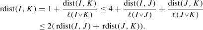
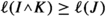
• (1) We denote $\ell =\ell (I)+\ell (J)+\ell (K)$. Since $\ell (J)\le \ell (I)$, we have and also 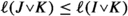. Moreover, . With this and $\textrm{dist}(I,K)\le \textrm{dist}(I,J)+\textrm{dist}(J,K) +\ell$, we can prove the first inequality:

  

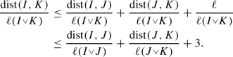
  Then

  

• (2) We now work on the second inequality. From $\textrm{dist}(I,J)\le \textrm{dist}(I,K)+\textrm{dist}(J,K)+\ell$ and $\textrm{dist}(J,K)\le \textrm{dist}(I,K)+\textrm{dist}(I,J)+\ell$ we have

  $$\begin{aligned} \textrm{dist}(I,K)\ge |\textrm{dist}(I,J)-\textrm{dist}(J,K)|-\ell . \end{aligned}$$

With this and , we get

As we saw before, , , and . Hence

Finally then

$\square$

Lemma 8.9

Given three cubes I, J, K such that $\ell (J)\le \ell (I)$ and $\ell (K)\le \ell (I)$, we have

(28)

Proof

From $\ell (J)\le \ell (I)$, and (26), we have $\textrm{dist}({\mathfrak {D}}_{I},J)=\textrm{dist}({\mathfrak {D}}_{I},{\mathfrak {D}}_{J})\le \textrm{dist}({\mathfrak {D}}_{I},K)+\textrm{dist}({\mathfrak {D}}_{J},K) +\ell (K)$. Then

$$\begin{aligned} \textrm{dist}({\mathfrak {D}}_{I},K)\ge \textrm{dist}({\mathfrak {D}}_{I},J)-\textrm{dist}({\mathfrak {D}}_{J},K)-\ell (K). \end{aligned}$$

If in addition $\ell (J)\le (K)$, then using that ${\mathfrak {D}}_{K}\subset {\overline{K}}$, the closure of K, we also have $\textrm{dist}({\mathfrak {D}}_{I},J)\le \textrm{dist}({\mathfrak {D}}_{I},K)+\textrm{dist}(J,K)+\ell (K) \le \textrm{dist}({\mathfrak {D}}_{I},K)+\textrm{dist}(J,{\mathfrak {D}}_{K})+\ell (K)$. With this

$$\begin{aligned} \textrm{dist}({\mathfrak {D}}_{I},K)\ge \textrm{dist}({\mathfrak {D}}_{I},J)-\textrm{dist}(J,{\mathfrak {D}}_{K})-\ell (K). \end{aligned}$$

Now, . If $\ell (K)\le \ell (J)$ we have . Meanwhile, if $\ell (J)\le \ell (K)$ we have . Then we denote $r_{J,K}=\textrm{dist}({\mathfrak {D}}_{J},K)$ if $\ell (K)\le \ell (J)$, and $r_{J,K}=\textrm{dist}(J,{\mathfrak {D}}_{K})$ if $\ell (J)\le \ell (K)$. With this and previous two inequalities, we get

Since $\ell (J)\le \ell (I)$, we have . Moreover, Since $\ell (K)\le \ell (I)$, we have . Then

With this

$\square$

Lemma 8.10

Given three cubes I, J, K such that $\ell (J)\le \ell (I)$, we have

Proof

We denote again .

• (a) We first assume that $\ell (K)\le \ell (J)$. Since $\ell (J)\le \ell (I)$, we have $\textrm{dist}({\mathfrak {D}}_{I},J)=\textrm{dist}({\mathfrak {D}}_{I},{\mathfrak {D}}_{J})\le \textrm{dist}({\mathfrak {D}}_{I},K)+\textrm{dist}({\mathfrak {D}}_{J},K) +\ell$, and also

  $$\begin{aligned} \textrm{dist}({\mathfrak {D}}_{J},K)&\le \textrm{dist}({\mathfrak {D}}_{I},K)+\textrm{dist}({\mathfrak {D}}_{I},{\mathfrak {D}}_{J})+\ell \\&=\textrm{dist}({\mathfrak {D}}_{I},K)+\textrm{dist}({\mathfrak {D}}_{I},J)+\ell . \end{aligned}$$

  Then we get

  $$\begin{aligned} \textrm{dist}({\mathfrak {D}}_{I},K)\ge |\textrm{dist}({\mathfrak {D}}_{I},J)-\textrm{dist}({\mathfrak {D}}_{J},K)|-\ell . \end{aligned}$$

  Moreover, from the assumptions $\ell (K)\le \ell (J)\le \ell (I)$, we have that , and 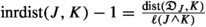. With this and previous inequality, we get

  

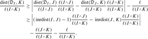
  Since $\ell (J)\le \ell (I)$, we have . Moreover, . Then

  

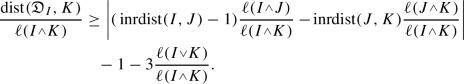
  With this and , we have

  

  which proves the inequality.

• (b) Now we assume that $\ell (J)\le \ell (K)\le \ell (I)$. Since ${\mathfrak {D}}_{K}\subset {\overline{K}}$, the closure of K, we have $\textrm{dist}({\mathfrak {D}}_{I},J)\le \textrm{dist}({\mathfrak {D}}_{I},K)+\textrm{dist}(J,K)+\ell \le \textrm{dist}({\mathfrak {D}}_{I},K)+\textrm{dist}(J,{\mathfrak {D}}_{K})+\ell$. Since $\ell (K)\le \ell (I)$, we get $\textrm{dist}(J,{\mathfrak {D}}_{K})\le \textrm{dist}({\mathfrak {D}}_{I},{\mathfrak {D}}_{K})+\textrm{dist}({\mathfrak {D}}_{I},J)+\ell =\textrm{dist}({\mathfrak {D}}_{I},K)+\textrm{dist}({\mathfrak {D}}_{I},J)+\ell$. With both things,

  $$\begin{aligned} \textrm{dist}({\mathfrak {D}}_{I},K)\ge |\textrm{dist}({\mathfrak {D}}_{I},J)-\textrm{dist}(J,{\mathfrak {D}}_{K})|-\ell . \end{aligned}$$

  Moreover, from the assumptions $\ell (J)\le \ell (I)$ and $\ell (J)\le \ell (K)$, we have that , and . With this and previous inequality, we have

  

  Since , and , we have

  

  Finally then since , we get as before

  

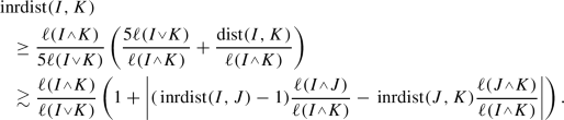
• (c) Finally we assume that $\ell (J)\le \ell (I)\le \ell (K)$. Since $\ell (I)\le \ell (K)$, we have $\textrm{dist}({\mathfrak {D}}_{I},J)\le \textrm{dist}({\mathfrak {D}}_{I},{\mathfrak {D}}_{K})+\textrm{dist}(J,{\mathfrak {D}}_{K})+\ell =\textrm{dist}(I,{\mathfrak {D}}_{K})+\textrm{dist}(J,{\mathfrak {D}}_{K})+\ell$, and $\textrm{dist}(J,{\mathfrak {D}}_{K})\le \textrm{dist}({\mathfrak {D}}_{I},{\mathfrak {D}}_{K})+\textrm{dist}({\mathfrak {D}}_{I},J)+\ell =\textrm{dist}(I,{\mathfrak {D}}_{K})+\textrm{dist}({\mathfrak {D}}_{I},J)+\ell$. Then

  $$\begin{aligned} \textrm{dist}(I, {\mathfrak {D}}_{K})\ge |\textrm{dist}({\mathfrak {D}}_{I},J)-\textrm{dist}(J,{\mathfrak {D}}_{K})|-\ell . \end{aligned}$$

From here we can work as in case b) since we only used the inequalites $\ell (J)\le \ell (I)$ and $\ell (J)\le \ell (K)$, , and , all of which still hold in this case. $\square$

The next result displays a direct relationship between the relative distance and the inner relative distance.

Lemma 8.11

Let $I,J\in {\mathcal {D}}$. Then

$$\begin{aligned} \textrm{ec}(I,J)\mathrm{\, inrdist}(I,J)\le \mathrm{\, rdist}(I,J)&\le 1 +\textrm{ec}(I,J)\mathrm{\, inrdist}(I,J). \end{aligned}$$

(29)

Proof

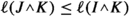
By symmetry we assume that $\ell (J)\le \ell (I)$. The upper estimate can be obtained directly from the definition: since ${\mathfrak {D}}_I\subset I$, and $\ell (J)\le \ell (I)$, we have

$$\begin{aligned} \mathrm{\, rdist}(I,J)&=1+\frac{\textrm{dist}(I,J)}{\ell (I)} \le 1+\frac{\textrm{dist}({\mathfrak {D}}_I,J)}{\ell (I)} \\&=1+\frac{(\mathrm{\, inrdist}(I,J)-1)\ell (J)}{\ell (I)} \\&=1-\frac{\ell (J)}{\ell (I)} +\frac{\ell (J)}{\ell (I)}\mathrm{\, inrdist}(I,J) \\&\le 1+\textrm{ec}(I,J)\mathrm{\, inrdist}(I,J). \end{aligned}$$

For the lower estimate, we divide in two cases. If $I\cap J=\emptyset$ then $\textrm{dist}({\mathfrak {D}}_I,J)=\textrm{dist}(I,J)$ and so we have with previous reasoning that

$$\begin{aligned} \mathrm{\, rdist}(I,J)&=1-\frac{\ell (J)}{\ell (I)} +\frac{\ell (J)}{\ell (I)}\mathrm{\, inrdist}(I,J) \\&\ge \textrm{ec}(I,J)\mathrm{\, inrdist}(I,J). \end{aligned}$$

On the other hand, if $J\subset I$, we have instead $\mathrm{\, rdist}(I,J)=1$ and also

$$\begin{aligned} \mathrm{\, inrdist}(I,J)=1+\frac{\textrm{dist}({\mathfrak {D}}_I,J)}{\ell (J)} \le 1+\frac{\ell (I)}{\ell (J)}. \end{aligned}$$

Then

$$\begin{aligned} \textrm{ec}(I,J)\mathrm{\, inrdist}(I,J)&=\frac{\ell (J)}{\ell (I)}\mathrm{\, inrdist}(I,J) \le \frac{\ell (J)}{\ell (I)}+1 \\&\le 2\lesssim \mathrm{\, rdist}(I,J). \end{aligned}$$

$\square$

8.4 An Estimate on the Function F

We end this section of technical results with a lemma that shows how to estimate the product of two outcomes of the auxiliary function F.

Lemma 8.12

Let $I,J\in {\mathcal {D}}$. Then

$$\begin{aligned} \sup _{K\in {\mathcal {D}}}\prod _{R\in \{I,J\}} F(R,K) \Bigg (\frac{\textrm{ec}(R,K)}{\mathrm{\, rdist}(R,K)}\Bigg )^{\delta '}&\lesssim F_{\theta }(I,J)^2, \end{aligned}$$

with where $L^\theta , S^\theta , D^\theta$ are given at the end of Sect. 4.2

Proof

According to Proposition 6.1, $F(I,J)=F_1(I,J)+F_2(I,J)$ where

and $F_2(I,J)=F_W(I)\delta (I,J)$. Then to prove the Lemma we need to estimate the following four products $F_i(I,K)F_j(J,K)$ for $i,j\in \{ 1,2\}$.

We first work with $F_1(I,K)F_1(J,K)$. From now, to simplify notation we assume without loss of generality that $\ell (J)\le \ell (I)$.

Since $\mathrm{\, rdist}(R,K)\ge 1$, we first we deal with the factor L by showing that

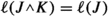• (a) If $\ell (J)\le \ell (K)$ then and . Then, since L is non-increasing, and $\textrm{ec}(R,K)\le 1$, we have

  

• (b) If $\ell (K)\le \ell (J)$, then we have

  

  (30)

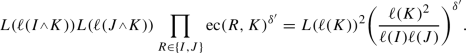
• (1) Now, if $\ell (K)\ge \ell (J)^{1-\theta }/2$, we can estimate (30) as

  $$\begin{aligned} L(\ell (K))^2\Bigg (\frac{\ell (K)^2}{\ell (I)\ell (J)}\Bigg )^{\delta '} \le L(\ell (J)^{1-\theta })^2 \le L^{\theta }(\ell (J))^2. \end{aligned}$$

• (2) If $\ell (K)\le \ell (J)^{1-\theta }/2$, we divide the study in two new cases.

• (2.a) If $\ell (J)\ge 1$, then

  $$\begin{aligned} L(\ell (K))^2\Bigg (\frac{\ell (K)^2}{\ell (I)\ell (J)} \Bigg )^{\delta '}&\le \frac{\ell (J)^{2(1-\theta )\delta '}}{\ell (I)^{\delta '}\ell (J)^{\delta '}} =\Bigg (\frac{\ell (J)}{\ell (I)}\Bigg )^{\delta '}\frac{1}{\ell (J)^{2\theta \delta '}} \\&\le \frac{1}{\ell (J)^{2\theta \delta '}} \approx \Bigg (\frac{1}{1+\ell (J)^{\theta \delta '}}\Bigg )^2 \le L^{\theta }(\ell (J))^2. \end{aligned}$$

• (2.b) If $\ell (J)\le 1$, we consider the last two cases:

  • If $\ell (K)\le \Bigg (\frac{ L_{\theta }(\ell (J))}{L(\ell (K))} \Bigg )^{1/\delta '}(\ell (I)\ell (J))^{\frac{1}{2}},$ then (30) can be estimated as

    $$\begin{aligned} L(\ell (K))^2\Bigg (\frac{\ell (K)^2}{\ell (I)\ell (J)} \Bigg )^{\delta '} \le L^{\theta }(\ell (J))^2. \end{aligned}$$

  • We now consider the case when $\ell (K)\ge \Bigg (\frac{ L^{\theta }(\ell (J))}{L(\ell (K))}\Bigg )^{1/\delta '} (\ell (I)\ell (J))^{\frac{1}{2}}.$ Since $L^{\theta }(x)\ge x^{1-\theta }$ for $0<x\le 1$ and $L(\ell (K))\lesssim 1$, we have

    $$\begin{aligned} \ell (K) > rsim L^{\theta }(\ell (J))^{1/\delta '}(\ell (I)\ell (J))^{\frac{1}{2}} > rsim \ell (J)^{\frac{1-\theta }{\delta '}}\ell (J)=\ell (J)^{1+\frac{1-\theta }{\delta '}}. \end{aligned}$$

    With this

    $$\begin{aligned} L(\ell (K))^2\Bigg (\frac{\ell (K)^2}{\ell (I)\ell (J)} \Bigg )^{\delta '}&\le L(\ell (K))^2 \\&\le L(\ell (J)^{1+\frac{1-\theta }{\delta '}})^2 \le L^\theta (\ell (J))^2. \end{aligned}$$

We continue with the factor S for which we show that

Since , and S is non-decreasing, we have

Since , , , and , we have

Then, since $S(\ell (J))\le S_\theta (\ell (J))$,

$$\begin{aligned} S(\ell (I)) S(\ell (J))\prod _{R\in \{I,J\}} \textrm{ec}(R,K)^{\delta '}&\lesssim S(\ell (I))\Bigg (\frac{\ell (J)}{\ell (I)+\ell (J)}\Bigg )^{\delta '}S^\theta (\ell (J)). \end{aligned}$$

We now prove that the first two factors are bounded by a constant times $S^\theta (\ell (J))$.

If $\ell (I)\le 2\ell (J)^{1-\theta }$, we have

$$\begin{aligned} S(\ell (I))\Bigg (\frac{\ell (J)}{\ell (I)+\ell (J)}\Bigg )^{\delta '} \lesssim S(2\ell (J)^{1-\theta })\le S^\theta (\ell (J)). \end{aligned}$$

On the other hand, if $\ell (I)>2\ell (J)^{^{1-\theta }}$, we get

$$\begin{aligned} S(\ell (I))\Bigg (\frac{\ell (J)}{\ell (I)+\ell (J)}\Bigg )^{\delta '}&\lesssim \Bigg (\frac{\ell (J)}{\ell (J)^{1-\theta }+\ell (J)}\Bigg )^{\delta '} \\&=\Bigg (\frac{\ell (J)^{\theta }}{\ell (J)^{\theta }+1}\Bigg )^{\delta '} \lesssim S^\theta (\ell (J)). \end{aligned}$$

In the last inequality we used the assumption that $S^{\theta }(x)\ge (\frac{x^\theta }{x^\theta +1})^{\delta '}$.

Now, to estimate the factor D, we show that

$$\begin{aligned} \prod _{R\in \{I,J\}} D(\mathrm{\, rdist}(\langle R,K\rangle , {\mathbb {B}})) \Bigg (\frac{\textrm{ec}(R,K)}{\mathrm{\, rdist}(R,K)}\Bigg )^{\delta '} \lesssim D_{\theta } (\mathrm{\, rdist}(\langle I,J\rangle , {\mathbb {B}}))^2 \end{aligned}$$

(31)

for $\theta \in (0,1)$ arbitrarily small. For this we define $k=\mathrm{\, rdist}(\langle I,J\rangle , {\mathbb {B}})$, fix $\theta$, and consider two cases.

A) If $\ell (K) +\textrm{dist}(K,\langle I,J\rangle )\le k^\theta (1+\ell (\langle I,J\rangle ))$, we first prove that

$$\begin{aligned} \min (\mathrm{\, rdist}(\langle I,K\rangle , {\mathbb {B}}), \mathrm{\, rdist}(\langle J,K\rangle , {\mathbb {B}})) > rsim \mathrm{\, rdist}(\langle I,J\rangle , {\mathbb {B}})^{1-\theta }. \end{aligned}$$

(32)

To show (32), we assume without loss of generality $\mathrm{\, rdist}(\langle J,K\rangle , {\mathbb {B}})\ge \mathrm{\, rdist}(\langle I,K\rangle , {\mathbb {B}})$. Since $I\subset \langle I,K\rangle \cap \langle I,J\rangle$, we have $\textrm{dist}(\langle I,K\rangle , \langle I,J\rangle )=0$. Then

$$\begin{aligned} \textrm{dist}(\langle I,J\rangle , {\mathbb {B}})&\le \textrm{dist}(\langle I,K\rangle , {\mathbb {B}}) +\textrm{dist}(\langle I,K\rangle , \langle I,J\rangle ) +\ell (\langle I,K\rangle )\nonumber \\&= \textrm{dist}(\langle I,K\rangle , {\mathbb {B}}) +\ell (\langle I,K\rangle ). \end{aligned}$$

(33)

We show now that

$$\begin{aligned} \ell (\langle I,K\rangle )&\lesssim k^\theta (1+\ell (\langle I,J\rangle )). \end{aligned}$$

First, since $\textrm{dist}(I, \langle I,J\rangle )=0$ and $\ell (I)\le \ell (\langle I,J\rangle )$, we have

$$\begin{aligned} \textrm{dist}(I,K)&\lesssim \textrm{dist}(K, \langle I,J\rangle ) +\textrm{dist}(I, \langle I,J\rangle ) +\ell (\langle I,J\rangle ) \\&= \textrm{dist}(K, \langle I,J\rangle ) +\ell (\langle I,J\rangle ). \end{aligned}$$

Then, since $k\ge 1$,

$$\begin{aligned} \ell (\langle I,K\rangle )&\lesssim \ell (I)+\ell (K)+\textrm{dist}(I,K) \\&\lesssim \ell (I)+\ell (K)+\textrm{dist}(K,\langle I,J\rangle )+\ell (\langle I,J\rangle ) \\&\lesssim \ell (K)+\textrm{dist}(K,\langle I,J\rangle )+2\ell (\langle I,J\rangle ) \\&\le 3 k^\theta (1+\ell (\langle I,J\rangle )), \end{aligned}$$

where the last inequality follows from the assumption. With this we continue the reasoning started at (33) as follows:

$$\begin{aligned} \textrm{dist}(\langle I,K\rangle , {\mathbb {B}})&\ge \textrm{dist}(\langle I,J\rangle , {\mathbb {B}}) -\ell (\langle I,K\rangle ) \\&\ge \textrm{dist}(\langle I,J\rangle , {\mathbb {B}}) -Ck^\theta (1+\ell (\langle I,J\rangle )). \end{aligned}$$

With all this, since $C>1$,

$$\begin{aligned} \mathrm{\, rdist}(\langle I,K\rangle , {\mathbb {B}})& > rsim 2+\frac{\textrm{dist}(\langle I,K\rangle , {\mathbb {B}})}{1+\ell (\langle I,K\rangle )} \\&\ge 2+\frac{C^{-1}\textrm{dist}(\langle I,K\rangle , \mathbb B)}{1+\ell (\langle I,K\rangle )} \\& > rsim 2+\frac{C^{-1}\textrm{dist}(\langle I,J\rangle , {\mathbb {B}}) - k^\theta (1+\ell (\langle I,J\rangle ))}{1+k^\theta (1+\ell (\langle I,J\rangle ))} \\& > rsim 1+\frac{C^{-1}\textrm{dist}(\langle I,J\rangle , {\mathbb {B}})}{1+k^\theta (1+\ell (\langle I,J\rangle ))} \\&\ge C^{-1}( 1+\frac{\textrm{dist}(\langle I,J\rangle , {\mathbb {B}})}{1+k^\theta (1+\ell (\langle I,J\rangle ))}). \end{aligned}$$

Now we note that $1+k^\theta (1+\ell (\langle I,J\rangle )\ge 1+\ell (\langle I,J\rangle )$ and so,

$$\begin{aligned} \mathrm{\, rdist}(\langle I,K\rangle , {\mathbb {B}})& > rsim \frac{1+\ell (\langle I,J\rangle )}{1+k^\theta (1+\ell (\langle I,J\rangle ))} \left( 1+\frac{\textrm{dist}(\langle I,J\rangle , {\mathbb {B}})}{1+\ell (\langle I,J\rangle )}\right) \\& > rsim \frac{1}{(1+\ell (\langle I,J\rangle ))^{-1}+k^\theta } \mathrm{\, rdist}(\langle I,J\rangle , {\mathbb {B}}) \\& > rsim \frac{1}{1+k^\theta } \mathrm{\, rdist}(\langle I,J\rangle , {\mathbb {B}}) \\&\ge \frac{1}{2k^\theta } \mathrm{\, rdist}(\langle I,J\rangle , {\mathbb {B}}) > rsim \mathrm{\, rdist}(\langle I,J\rangle , {\mathbb {B}})^{1-\theta }, \end{aligned}$$

by the definition of k. This proves the claim at (32).

Hence, since $\prod _{R\in \{I,J\}} \Bigg (\frac{\textrm{ec}(R,K)}{\mathrm{\, rdist}(R,K)}\Bigg )^{\delta '}\le 1$ and D is non-increasing, the right hand side of (31) can be bounded by

$$\begin{aligned} D(\mathrm{\, rdist}(\langle I,K\rangle , {\mathbb {B}})) D(\mathrm{\, rdist}(\langle J,K\rangle , {\mathbb {B}}))&\lesssim D(\mathrm{\, rdist}(\langle I,J\rangle , {\mathbb {B}})^{1-\theta })^2 \\&\le D^{\theta }(\mathrm{\, rdist}(\langle I,J\rangle , {\mathbb {B}}))^2. \end{aligned}$$

B) On the other hand, if $\ell (K)+\textrm{dist}(K,\langle I,J\rangle )>k^\theta (1+\ell (\langle I,J\rangle ))$, since $R\subset \langle I,J\rangle$ for both $R\in \{I,J\}$, we have

$$\begin{aligned} \ell (\langle R,K\rangle )& > rsim \ell (K)+\textrm{dist}(R,K) \\&\ge \ell (K)+\textrm{dist}(\langle I,J\rangle ,K) \\&\ge k^\theta (1+\ell (\langle I,J\rangle )). \end{aligned}$$

Moreover,

With this and $D(x)\lesssim 1$, the right hand side of (31) is bounded by

In the last inequality we used the assumption that $D^{\theta }(x)\ge (1+x^{\theta \delta '})^{-1}$ and the fact that $\mathrm{\, rdist}(\langle I,J\rangle , {\mathbb {B}})\ge 1$.

The work developed for the factors L, S, and D finally shows that $F_1(I,K)F_1(J,K)\lesssim F_\theta (I)^2.$ The next terms to be considered are

$$\begin{aligned} F_2(I,K)F_2(J,K)&= F_W(I,K)\delta (I,K)F_W(J,K)\delta (J,K) \\&=F_W(I)^2\delta (I,J)\le F_\theta (I,J)^2, \end{aligned}$$

and

The estimate for $F_2(I,K)F_1(J,K)$ follows by symmetry. $\square$

9 Bump Estimates for Powers of Compact Calderón–Zygmund Operators

We remind that for T a Calderón–Zygmund operator with associated function F and such that $T1=T^*1=0$, we have

$$\begin{aligned} |\langle T\psi _{I},\psi _{J}\rangle | \lesssim A_{I,J}F(I,J) \end{aligned}$$

where $A_{I,J}=\textrm{ec}(I,J)^{\frac{d}{2}+\delta }\mathrm{\, rdist}(I,J)^{-(d+\delta )}$ if say $\mathrm{\, rdist}(I,J)>10$, while $A_{I,J}=\textrm{ec}(I,J)^{\frac{d}{2}}\mathrm{\, inrdist}(I,J)^{-\delta }$ otherwise.

We now prove the following extension of previous inequality to powers of $T^*T$.

Theorem 9.1

Let T be a Calderón–Zygmund operator with associated function F such that $T1=T^*1=0$. For every $n\ge 0$,

$$\begin{aligned} |\langle (T^*T)^{2^n}\psi _{I},\psi _{J}\rangle | \lesssim A_{I,J}'F_\theta (I,J)^{2^{n+1}} \end{aligned}$$

where $F_\theta$ is defined in Lemma 8.12, $A_{I,J}'=\textrm{ec}(I,J)^{\frac{d}{2}+\delta '}\mathrm{\, rdist}(I,J)^{-(d+\delta ')}$ if $\mathrm{\, rdist}(I,J)>10$, and $A_{I,J}=\textrm{ec}(I,J)^{(1-\theta )\frac{d}{2}}\mathrm{\, inrdist}(I,J)^{-\delta '}$ otherwise, with $\delta '=(1-\theta )\delta$ such that $\theta \in (0,1)$ can be arbitrarily chosen.

We note that exactly the same ideas can be used to prove the following result:

Corollary 9.2

Let $T_1$ and $T_2$ be two Calderón–Zygmund operators with associated functions $F_i$ such that $T_i1=T_i^*1=0$. Then

$$\begin{aligned} |\langle T_1T_2\psi _{I},\psi _{J}\rangle | \lesssim A_{I,J}'F_\theta (I,J). \end{aligned}$$

Proof

Let $e\in {\mathbb {Z}}$, $m\in {\mathbb {N}}$ be such that $J\in I_{e,m}$, that is, $\ell (I)=2^e\ell (J)$ and $m<\mathrm{\, rdist}(I,J)\le m+1$. By symmetry, we can assume that $\ell (J)\le \ell (I)$, namely, that $e\ge 0$.

We prove the inequality by induction, starting with the case $n=0$, that is, we show that

$$\begin{aligned} |\langle T^*T\psi _{I},\psi _{J}\rangle | \lesssim A_{e,m}F_\theta (I,J)^{2}. \end{aligned}$$

By the orthogonality properties of the Haar wavelets in (9), we have

$$\begin{aligned} \langle T^*T\psi _{I},\psi _{J}\rangle&=\langle T\psi _{I},T\psi _{J}\rangle =\sum _{K,K'\in {{\mathcal {D}}}} \langle T\psi _{I},\psi _{K}\rangle \langle T\psi _{J},\psi _{K'}\rangle \langle \psi _K,\psi _{K'}\rangle \\&=\sum _{K\in {{\mathcal {D}}}}\sum _{\begin{array}{c} K'\in {\mathcal D}\\ \widehat{K'}={\widehat{K}} \end{array}} \langle T\psi _{I},\psi _{K}\rangle \langle T\psi _{J},\psi _{K'}\rangle (\delta (K,K')-2^{-d}) . \end{aligned}$$

We now enumerate the $2^d$ cubes $K'\in \textrm{ch}{{\widehat{K}}}$, so that

$$\begin{aligned} \langle T^*T\psi _{I},\psi _{J}\rangle&=\sum _{i=1}^{2^d}\sum _{K\in {{\mathcal {D}}}}(\delta (K,K_i)-2^{-d}) \langle T\psi _{I},\psi _{K}\rangle \langle T\psi _{J},\psi _{K_i}\rangle . \end{aligned}$$

Since $|\delta (K,K')-2^{-d}|\le 2$, we just need to estimate the inner sum uniformly in the index i. Since the same argument works for any cube $K_i$, to simplify notation we only show the work when $K_i=K$.

We parametrize the cubes K according to eccentricity and relative size with respect to J: for each $e',m'$, we rewrite the parameterization used in Theorem 7.1 as

$$\begin{aligned} J_{e,m}=J_{e,m,0}=\{ I\in {{\mathcal {D}}}:\ell (I)=2^{e}\ell (J), m\le \mathrm{\, rdist}(I,J)< m+1 \}, \end{aligned}$$

and when $m\le 3$

$$\begin{aligned} J_{e,m,k}=\{ I\in J_{e,m}: k\le \mathrm{\, inrdist}(I,J)<k+1\}. \end{aligned}$$

We then consider the cubes . Then

$$\begin{aligned} |\langle T^*T\psi _{I},\psi _{J}\rangle |&\approx \left| \sum _{e'\in {\mathbb {Z}}}\sum _{m'\in {\mathbb {N}}} \sum _{K\in J_{e',m'}} \langle T\psi _{I},\psi _{K}\rangle \langle T\psi _{J},\psi _{K}\rangle \right| . \end{aligned}$$

(34)

We divide the long proof into multiple cases depending on the relative sizes and distances of I, J, and K.

1) We first consider the case $\mathrm{\, rdist}(I,J)\ge m>3$, which we divide into three sub-cases depending on the relative distances of K with respect to J and I. We aim to prove that

$$\begin{aligned} |\langle T^*T\psi _{I},\psi _{J}\rangle |&\lesssim \textrm{ec}(I,J)^{\frac{d}{2}+\delta } \mathrm{\, rdist}(I,J)^{-(d+\delta )}F_\theta (I,J)\nonumber \\&\approx 2^{-e(\frac{d}{2}+\delta )} m^{-(d+\delta )}F_\theta (I,J). \end{aligned}$$

(35)

a) When $\mathrm{\, rdist}(J,K)>3$ and $\mathrm{\, rdist}(I,K)>3$, we can bound the terms in (67) corresponding to this case as follows:

$$\begin{aligned}&\sum _{e'\in {\mathbb {Z}}} \sum _{\begin{array}{c} m'\in {\mathbb {N}}\\ m'>3 \end{array}} \sum _{K\in J_{e',m'}} |\langle T\psi _{I},\psi _{K}\rangle | |\langle T\psi _{J},\psi _{K}\rangle |\nonumber \\&\quad \le \sum _{e'\in {\mathbb {Z}}}\sum _{m'\in {\mathbb {N}}} \sum _{K\in J_{e',m'}} \textrm{ec}(I,K)^{\frac{d}{2}+\delta }\mathrm{\, rdist}(I,K)^{-(d+\delta )}F(I,K)\nonumber \\&\qquad \textrm{ec}(J,K)^{\frac{d}{2}+\delta } \mathrm{\, rdist}(J,K)^{-(d+\delta )}F(J,K). \end{aligned}$$

(36)

Since $\ell (J)\le \ell (I)$, by Lemma 8.7,

(37)

We note that $\ell (I)=2^e\ell (J)$ and $\ell (J)=2^{e'}\ell (K)$ imply $\ell (I)=2^{e+e'}\ell (K)$. Then we subdivide in three more cases now depending on the eccentricities.

a.1) If $\ell (K)\le \ell (J)$ we have $e'\ge 0$ and then $e+e'\ge 0$. Then the inequality in (37) stands as

$$\begin{aligned} \mathrm{\, rdist}(I,K)& > rsim 1+\left| \mathrm{\, rdist}(I,J)-\frac{\ell (J)}{\ell (I)} \mathrm{\, rdist}(J,K)\right| > rsim 1+|m-2^{-e}m'|. \end{aligned}$$

The last inequality is proved as follows. We denote the middle expression as $1+|\cdot |$. Since $m<\mathrm{\, rdist}(I,J)\le m+1$, and $m'<\mathrm{\, rdist}(J,K)\le m'+1$, we have

$$\begin{aligned} 1+|\cdot |&\ge 1+\mathrm{\, rdist}(I,J)-\frac{\ell (J)}{\ell (I)} \mathrm{\, rdist}(J,K) \\&\ge 1+m-2^{-e}(m'+1)\ge m-2^{-e}m'. \end{aligned}$$

On the other hand,

$$\begin{aligned} 1+|\cdot |&\ge 1+\frac{\ell (J)}{\ell (I)}\mathrm{\, rdist}(J,K)-\mathrm{\, rdist}(I,J) \\&\ge 1+2^{-e}m'-(m+1)= 2^{-e}m'-m. \end{aligned}$$

With both things, $1+|\cdot | \ge |m-2^{-e}m'|$, and so

$$\begin{aligned} 1+|\cdot |&\ge 2^{-1}(2+|\mathrm{\, rdist}(I,J)-\frac{\ell (J)}{\ell (I)}\mathrm{\, rdist}(J,K)|) \\&\ge 2^{-1}(1+|m-2^{-e}m'|). \end{aligned}$$

as claimed. Since $\textrm{ec}(I,K)=\frac{\ell (K)}{\ell (I)}=2^{-(e+e')}$, and $\textrm{ec}(J,K)=\frac{\ell (K)}{\ell (J)}=2^{-e'}$, the terms in (36) related to this case can be written as

$$\begin{aligned} \sum _{e'\ge 0}\sum _{m'>3} \sum _{K\in J_{e',m'}}&2^{-(e+e')(\frac{d}{2}+\delta )} (1+|m-2^{-e} m'|)^{-(d+\delta )}F(I,K)\\&2^{-e'(\frac{d}{2}+\delta )}m'^{-(d+\delta )} F(J,K). \end{aligned}$$

We denote $\delta _\theta =(1-\theta )\delta$. By using that the cardinality of $J_{e',m'}$ is comparable to $2^{e'd}m'^{d-1}$, we can bound previous expression by

$$\begin{aligned}&\sum _{e'\ge 0}\sum _{m'>3} \hspace{5.0pt}2^{e'd}m'^{d-1} \hspace{5.0pt}2^{-(e+e')(\frac{d}{2}+\delta _\theta )} (1+|m-2^{-e} m'|)^{-(d+\delta _\theta )} \\&\qquad 2^{-e'(\frac{d}{2}+\delta _\theta )}m'^{-(d+\delta _\theta )} \sup _{K\in \mathcal D}\prod _{R\in \{I,J\}}F(R,K) \Bigg (\frac{\textrm{ec}(R,K)}{\mathrm{\, rdist}(R,K)}\Bigg )^{\theta \delta } \\&\quad \lesssim F_\theta (I,J) 2^{-e(\frac{d}{2}+\delta )}\sum _{e'\ge 0}2^{-e'2\delta }\hspace{-.1cm} \sum _{m'>3}(1+|m-2^{-e} m'|)^{-(d+\delta )} m'^{-(d+\delta )}m'^{d-1}. \end{aligned}$$

The last inequality follows from Lemma 8.12, by which we have

$$\begin{aligned} \sup _{K\in {\mathcal {D}}}\prod _{R\in \{I,J\}}F(R,K) \Bigg (\frac{\textrm{ec}(R,K)}{\mathrm{\, rdist}(R,K)}\Bigg )^{\theta \delta }&\lesssim F_\theta (I,J). \end{aligned}$$

To simplify notation, we denote $\delta _\theta$ as $\delta$ again. Now, we note that the cardinality of the integers inside the ball of radius $m'$ is comparable to $m'^{d-1}$. Then we denote $\bar{m}=me_{1}=(m,0,\ldots , 0)$ and we use the second inequality of Lemma 8.2 with $\lambda =2^{-e}\le 1$ (or rather Remark 8.3) to rewrite and estimate the inner sum as follows:

$$\begin{aligned}&\sum _{m'>3}(1+|m-2^{-e} m'|)^{-(d+\delta )} (1+m')^{-(d+\delta )}m'^{d-1} \\&\quad \lesssim \sum _{\begin{array}{c} {\bar{m}}'\in {\mathbb {Z}}^d\\ \max _{i=1,\ldots ,d}|{\bar{m}}_i'|>3 \end{array}}(1+|{\bar{m}}-2^{-e} {\bar{m}}'|)^{-(d+\delta )}(1+|\bar{m}'|)^{-(d+\delta )} \\&\quad \lesssim (1+m)^{-(d+\delta )}. \end{aligned}$$

With this, the terms in (36) corresponding to this case can be bounded by a constant times

$$\begin{aligned} F_\theta (I,J)&2^{-e(\frac{d}{2}+\delta )}\hspace{-.1cm} \sum _{e'\ge 0}2^{-e'2\delta } (1+m)^{-(d+\delta )}\hspace{-.1cm} \lesssim 2^{-e(\frac{d}{2}+\delta )}(1+m)^{-(d+\delta )}F_\theta (I,J). \end{aligned}$$

a.2) When $\ell (J)\le \ell (K)\le (I)$ we have that $e'\le 0$ and $e+e'\ge 0$. Then (37) holds as

$$\begin{aligned} \mathrm{\, rdist}(I,K) > rsim 1+|\mathrm{\, rdist}(I,J)-\frac{\ell (K)}{\ell (I)}\mathrm{\, rdist}(J,K)| > rsim 1+|m-2^{-(e+e')}m'|, \end{aligned}$$

where the last inequality can be proved as we did before.

Now, $\textrm{ec}(I,K)=\frac{\ell (K)}{\ell (I)}=2^{-(e+e')}$, $\textrm{ec}(J,K)=\frac{\ell (J)}{\ell (K)}=2^{e'}$ and the cardinality of $J_{e',m'}$ is comparable to $m'^{d-1}$. These are the only changes with respect previous case. Then by Lemma 8.12

$$\begin{aligned}&\sum _{-e\le e'\le 0}\sum _{m'>3} 2^{-(e+e')(\frac{d}{2}+\delta )} (1+|m-2^{-(e+e')} m'|)^{-(d+\delta )} \\&\qquad 2^{e'(\frac{d}{2}+\delta )}m'^{-(d+\delta )}m'^{d-1} F(I,K)F(J,K) \\&\quad \le F_\theta (I,J) 2^{-e(\frac{d}{2}+\delta )}\sum _{-e\le e'\le 0} \sum _{m'>3}(1+|m-2^{-(e+e')} m'|)^{-(d+\delta )}m'^{-(1+\delta )}. \end{aligned}$$

By the second inequality of Lemma 8.2 with $\lambda =2^{-(e+e')}\le 1$

$$\begin{aligned} \sum _{m'>3}(1+|m-2^{-(e+e')} m'|)^{-(d+\delta )}m'^{-(1+\delta )}&\lesssim (1+m)^{-(d+\delta )}. \end{aligned}$$

With this we get the bound

$$\begin{aligned}&F_\theta (I,J) 2^{-e(\frac{d}{2}+\delta )}\sum _{-e\le e'\le 0} (1+m)^{-(d+\delta )} \\&\quad \le F_\theta (I,J) 2^{-e(\frac{d}{2}+\delta )}e (1+m)^{-(d+\delta )}\\&\quad \lesssim 2^{-e(\frac{d}{2}+\delta ' )} (1+m)^{-(d+\delta )}F_\theta (I,J) \end{aligned}$$

for $\delta '<\delta$.

a.3) Finally, when $\ell (J)\le \ell (I)\le \ell (K)$ we have $e'\le 0$ and $e+e'\le 0$ and thus, (37) stays as

$$\begin{aligned} \mathrm{\, rdist}(I,K) > rsim 1+|\frac{\ell (I)}{\ell (K)}\mathrm{\, rdist}(I,J)-\mathrm{\, rdist}(J,K)| > rsim 1+|2^{e+e'}m-m'|, \end{aligned}$$

where the last inequality is proved as we did in case a).

Moreover, $\textrm{ec}(I,K)=\frac{\ell (I)}{\ell (K)}=2^{e+e'}$, $\textrm{ec}(J,K)=\frac{\ell (J)}{\ell (K)}=2^{e'}$ and the cardinality of $J_{e',m'}$ is comparable to $m'^{d-1}$. Then, with similar ideas as before, we have

$$\begin{aligned}&\sum _{e'\le -e\le 0}\sum _{m'>3} 2^{(e+e')(\frac{d}{2}+\delta )} (1+|2^{e+e'}m-m'|)^{-(d+\delta )} \\&\qquad 2^{e'(\frac{d}{2}+\delta )}m'^{-(d+\delta )}m'^{d-1}F(I,K)F(J,K) \\&\quad \lesssim F_\theta (I,J) 2^{e(\frac{d}{2}+\delta )}\hspace{-.2cm}\sum _{e'\le -e\le 0}2^{e'(d+2\delta )} \sum _{\begin{array}{c} m'\in {\mathbb {Z}}^d\\ |m_i'|>3 \end{array}}(1+|2^{e+e'}m- m'|)^{-(d+\delta )}m'^{-(d+\delta )}\\&\quad \lesssim F_\theta (I,J) 2^{e(\frac{d}{2}+\delta )}\sum _{e'\le -e\le 0}2^{e'(d+2\delta )} (1+2^{e+e'}m)^{-(d+\delta )}, \end{aligned}$$

where in the last step we used the first inequality in Lemma 8.2 with $\lambda =2^{e+e'}$. Since $m\ge 1$, we now estimate the last expression by

$$\begin{aligned}&F_\theta (I,J) 2^{e(\frac{d}{2}+\delta )} \sum _{e'\le -e\le 0}2^{e'(d+2\delta )} 2^{-(e+e')(d+\delta )}m^{-(d+\delta )} \\&\quad \lesssim F_\theta (I,J) 2^{-e\frac{d}{2}}(1+m)^{-(d+\delta )} \sum _{e'\le -e\le 0}2^{e'\delta } \\&\quad \lesssim 2^{-e(\frac{d}{2}+\delta )} (1+m)^{-(d+\delta )}F_\theta (I,J). \end{aligned}$$

b) We continue with the case $\mathrm{\, rdist}(I,K)\le 3$ and $\mathrm{\, rdist}(J,K)>3$. Note that the first inequality and $\mathrm{\, rdist}(I,J)$ being large do not imply that $\mathrm{\, rdist}(J,K)$ is large. We can bound the terms in (67) corresponding to this case as follows:

$$\begin{aligned}&\sum _{e'\in {\mathbb {Z}}} \sum _{\begin{array}{c} m'\in \mathbb N\\ m'>3 \end{array}} \sum _{K\in J_{e',m'}} |\langle T\psi _{I},\psi _{K}\rangle | |\langle T\psi _{J},\psi _{K}\rangle |\nonumber \\&\quad \le \sum _{e'\in {\mathbb {Z}}}\sum _{m'\in {\mathbb {N}}} \sum _{K\in J_{e',m'}} \textrm{ec}(I,K)^{\frac{d}{2}}\mathrm{\, inrdist}(I,K)^{-\delta }F(I,K)\nonumber \\&\qquad \textrm{ec}(J,K)^{\frac{d}{2}+\delta } \mathrm{\, rdist}(J,K)^{-(d+\delta )}F(J,K). \end{aligned}$$

(38)

Then we consider the same three sub-cases as before depending on the eccentricities.

b.1) If $\ell (K)\le \ell (J)$ we have as before $e'\ge 0$ and $e+e'\ge 0$, and

$$\begin{aligned} 3&\ge \mathrm{\, rdist}(I,K) > rsim 1+\left| \mathrm{\, rdist}(I,J)-\frac{\ell (J)}{\ell (I)} \mathrm{\, rdist}(J,K)\right| \\&\ge (12)^{-1}(1+|m-2^{-e}m'|), \end{aligned}$$

as we saw in Lemma 8.7 and case (a.1). Then $|m-2^{-e}m'|\le 35$ and so $2^{-e}m'\ge m-35\ge m/2$ provided that $m\ge 70$. With this, $\mathrm{\, rdist}(J,K)\ge m' > rsim 2^em$.

Now the cubes $K\in J_{e',m'}$ need to be parametrized in terms of their relative size and distance with respect to I. Namely, we write $K\in I_{e+e',m,k}$. Then we define $I\!J=J_{e',m'}\cap I_{e+e',m,k}$, where we omit the parameters in the notation. For $K\in I\!J$ we have $k<\mathrm{\, inrdist}(I,K)\le k+1$.

Then, since $\textrm{ec}(I,K)=2^{-(e+e')}$, and $\textrm{ec}(J,K)=2^{-e'}$, the expression in (38) is bounded by a constant times

$$\begin{aligned}&\sum _{e'\ge 0} \sum _{k=1}^{2^{e+e'}} \sum _{K\in I\!J} 2^{-(e+e')\frac{d}{2}}{k}^{-\delta } F(I,K) 2^{-e'(\frac{d}{2}+\delta )} ({2^em})^{-(d+\delta )} F(J,K) \nonumber \\&\quad \lesssim 2^{-e(\frac{3d}{2}+\delta )}m^{-(d+\delta )}F_\theta (I,J) \sum _{e'\ge 0} \sum _{k=1}^{2^{e+e'}} \sum _{K\in I\!J} k^{-\delta } 2^{-e'(d+\delta )}. \end{aligned}$$

(39)

We remind that the last inequality follows from Lemma 8.12 because

The cardinality of $I\!J$ is bounded by the cardinalities of $J_{e',m'}$ and $I_{e+e',m,k}$, and so it can be estimated by

$$\begin{aligned} \min (2^{e'(d-1)}m'^{d-1}, 2^{(e+e')(d-1)})&=2^{e'(d-1)}\min (m', 2^{e})^{d-1} \\&\le 2^{e'(d-1)}\min (2^e (m+35), 2^{e})^{d-1} \\&=2^{(e+e')(d-1)}. \end{aligned}$$

Moreover, we note that for any $r>0$ and $\gamma =\frac{1}{1+\delta }$,

$$\begin{aligned} \sum _{k=1}^{2^{r}} k^{-\delta }&=\sum _{k=1}^{2^{\gamma r}-1} {k}^{-\delta } +\sum _{k=2^{\gamma r}}^{2^{r}} k^{-\delta } \lesssim 2^{\gamma r} +2^{-\delta \gamma r}2^{r} \lesssim 2^{\frac{r}{1+\delta }}. \end{aligned}$$

(40)

With this $\sum _{k=1}^{2^{e+e'}} k^{-\delta }\lesssim 2^{\frac{e+e'}{1+\delta }}$.

Then we can estimate the inner sum in (39) by

$$\begin{aligned} \sum _{e'\ge 0} 2^{-e'(d+\delta )} \sum _{k=1}^{2^{e+e'}} k^{-\delta } |I\!J|&\lesssim \sum _{\begin{array}{c} e'\ge 0 \end{array}} 2^{-e'(d+\delta ) }2^{(e+e')(d-1)} 2^{(e+e')\frac{1}{1+\delta }} \\&=2^{e(d-1+\frac{1}{1+\delta })} \sum _{\begin{array}{c} e'\ge 0 \end{array}} 2^{-e'(1+\delta -\frac{1}{1+\delta })} \\&\lesssim 2^{e(d-1+\frac{1}{1+\delta })}, \end{aligned}$$

since $1+\delta -\frac{1}{1+\delta }>0$. With this, the expression in (39) is bounded by

$$\begin{aligned} 2^{-e(\frac{d}{2}+\delta +1-\frac{1}{1+\delta })}m^{-(d+\delta )}F_\theta (I,J) \le 2^{-e(\frac{d}{2}+\delta )}m^{-(d+\delta )}F_\theta (I,J), \end{aligned}$$

since $1-\frac{1}{1+\delta }>0$.

b.2) When $\ell (J)\le \ell (K)\le (I)$ we have $e'\le 0$ and $e+e'\ge 0$. Then

$$\begin{aligned} 3&\ge \mathrm{\, rdist}(I,K) > rsim 1+|\mathrm{\, rdist}(I,J)-\frac{\ell (K)}{\ell (I)}\mathrm{\, rdist}(J,K)| \\& > rsim 1+|m-2^{-(e+e')}m'|, \end{aligned}$$

which implies $|m-2^{-(e+e')}m'|\lesssim 1$, that is $m'\approx 2^{e+e'}m$ as long as $m\ge 70$. Then $\mathrm{\, rdist}(J,K) > rsim 2^{e+e'}m$. This, together with $\textrm{ec}(I,K)=2^{-(e+e')}$, $\textrm{ec}(J,K)=2^{e'}$, are the only changes with respect previous case and so, the similar work leads to

$$\begin{aligned}&\sum _{-e\le e'\le 0} \sum _{k=1}^{2^{e+e'}} \sum _{K\in I\!J} 2^{-(e+e')\frac{d}{2}}k^{-\delta } F(I,K) 2^{e'(\frac{d}{2}+\delta )} ({2^{e+e'}m})^{-(d+\delta )} F(J,K) \nonumber \\&\quad \lesssim 2^{-e(\frac{3d}{2}+\delta )}m^{-(d+\delta )} F_{\theta }(I,J) \sum _{-e\le e'\le 0} \sum _{k=1}^{2^{e+e'}} \sum _{K\in I\!J} k^{-\delta } 2^{-e'd}. \end{aligned}$$

(41)

The cardinality of $J_{e',m'}$ is now comparable to $m'^{d-1}$, but this stills provides the same estimate for the cardinality of $I\!J$ as we see:

$$\begin{aligned} \min (m'^{d-1}, 2^{(e+e')(d-1)})&=\min (m', 2^{e+e'})^{d-1} \\&\le \min (2^{e+e'}(m+35), 2^{e+e'})^{d-1} \\&=2^{(e+e')(d-1)}. \end{aligned}$$

Moreover, $\sum _{k=1}^{2^{e+e'}} k^{-\delta }\lesssim 2^{(e+e')\frac{1}{1+\delta }}$. Then the inner sum at (41) can be estimated by

$$\begin{aligned} \sum _{-e\le e'\le 0} 2^{-e'd } 2^{(e+e')(d-1)}2^{(e+e')\frac{1}{1+\delta }}&=2^{e(d-1+\frac{1}{1+\delta })} \sum _{-e\le e'\le 0} 2^{-e'(1-\frac{1}{1+\delta })} \\&\lesssim 2^{e(d-1+\frac{1}{1+\delta })} 2^{e(1-\frac{1}{1+\delta })}=2^{ed}, \end{aligned}$$

since $1 -\frac{1}{1+\delta }>0$ and $e'\le 0$. Then the expression in (41) is bounded by

$$\begin{aligned} 2^{-e(\frac{3d}{2}+\delta )}m^{-(d+\delta )}F_\theta (I,J)2^{ed} = 2^{-e(\frac{d}{2}+\delta )}m^{-(d+\delta )}F_\theta (I,J). \end{aligned}$$

b.3) Finally, when $\ell (J)\le \ell (I)\le \ell (K)$ we have $e'\le 0$ and $e+e'\le 0$ and thus,

$$\begin{aligned} 3\ge \mathrm{\, rdist}(I,K) > rsim 1+|\frac{\ell (I)}{\ell (K)}\mathrm{\, rdist}(I,J)-\mathrm{\, rdist}(J,K)| > rsim 1+|2^{e+e'}m-m'|, \end{aligned}$$

which implies $|m-2^{e+e'}m'|\lesssim 1$, and so $m'\approx 2^{-(e+e')}m$ for $m\ge 70$. With this $\mathrm{\, rdist}(J,K) > rsim 2^{-(e+e')}m$.

The cardinality of $I_{e+e',m,k}$ is now bounded by a constant times $2^{M(e+e')(d-1)}=1$, where as in the proof of Theorem 7.1, we denote $M(e)=\max (e,0)$. Moreover, for any fixed cube J there is only one value of $1\le k_0\le 2^{|e+e'|}$ such that $I_{e+e',m,k}$ is non empty. Then

$$\begin{aligned}&\sum _{e'\le -e} \sum _{K\in I_{e+e',m,k}} 2^{(e+e')\frac{d}{2}} k_0'^{-\delta } F(I,K) 2^{e'(\frac{d}{2}+\delta )} ({2^{-(e+e')}m})^{-(d+\delta )} F(J,K) \nonumber \\&\quad \lesssim 2^{e(\frac{3d}{2}+\delta )}m^{-(d+\delta )} F_\theta (I,J) \sum _{e'\le -e} \sum _{K\in I\!J} 2^{e'2(d+\delta )}, \end{aligned}$$

(42)

where we used Lemma 8.12 once more.

Since the cardinality of $J_{e',m',k'}$ is bounded by 1, we have that the cardinality of $I\!J$ is estimated by $\min (m'^{d-1}, 1)=1$.

Then the expression in (42) is bounded by

$$\begin{aligned} 2^{e(\frac{3d}{2}+\delta )}m^{-(d+\delta )} F_\theta (I,J) 2^{-e2(d+\delta )} = 2^{-e(\frac{d}{2}+\delta )}m^{-(d+\delta )}F_\theta (I,J). \end{aligned}$$

c) Now we consider the case when $\mathrm{\, rdist}(J,K)< m'+1\le 4$ (regardless of $\mathrm{\, rdist}(I,K)$). As in case b), we cannot conclude that $\mathrm{\, rdist}(I,K)$ is large. But by Lemma 8.7 and the inequality , we have

(43)

We now define $\Delta _{e_0'} J=\{ x\in J: \textrm{dist}(x, \partial J)\le 2^{e_0'}\}$. Since $|\Delta _{e_0'} J|\lesssim 2^{e_0'(d-1)}|J|$,

$$\begin{aligned} \Vert \psi _J\Vert _{L^2(\Delta _{e_0'} J)}^2&=|J|^{-1}\int _{\Delta _{e_0'} J} (\mathbb {1}_{J}(x) -2^{-d}\mathbb {1}_{{\widehat{J}}}(x))^2 dx \\&= |J|^{-1}(1-2^{-d})^2|\Delta _{e_0'} J| \lesssim 2^{e_0'(d-1)}. \end{aligned}$$

We then fix a negative parameter $e_0'$ so that

$$\begin{aligned} \Vert \psi _J\Vert _{L^2(\Delta _{e_0'} J)}\lesssim 2^{e_0'\frac{d-1}{2}}<\Vert T\Vert ^{-2}2^{-e(\frac{d}{2}+\delta )} m^{-(d+\delta )}F_\theta (I,J) \end{aligned}$$

(44)

and we divide the study in two cases.

c.1) When $\ell (K)\le 2^{e_0'}\ell (J)$, we can reason as in cases a) and b). Since $\ell (K)\le \ell (J)\le \ell (I)$, we have that

$$\begin{aligned} \mathrm{\, rdist}(I,K)& > rsim 1+\frac{\ell (J)}{\ell (K)}\mathrm{\, rdist}(I,J) \ge 1+m \ge m\ge 3. \end{aligned}$$

(45)

We note that $\ell (K)\le 2^{e_0'}\ell (J)=2^{e_0'+e'}\ell (K)$ and so, $e'\ge -e_0'\ge 0$. Moreover $e+e'\ge 0$. We then can bound the terms in (67) corresponding to this case as follows:

$$\begin{aligned}&\sum _{\begin{array}{c} e'\in {\mathbb {Z}}\\ e'\ge 0 \end{array}} \sum _{\begin{array}{c} m'\in {\mathbb {N}}\\ m'\le 3 \end{array}} \sum _{K\in J_{e',m'}} |\langle T\psi _{I},\psi _{K}\rangle | |\langle T\psi _{J},\psi _{K}\rangle | \nonumber \\&\quad \le \sum _{\begin{array}{c} e'\in {\mathbb {Z}}^{+}\\ 1\le m'\le 3 \end{array}} \sum _{k=1}^{2^{e'}} \sum _{K\in J_{e',m',k'}} \hspace{-.4cm} \textrm{ec}(I,K)^{\frac{d}{2}+\delta } \mathrm{\, rdist}(I,K)^{-(d+\delta )}F(I,K) \nonumber \\&\qquad \textrm{ec}(J,K)^{\frac{d}{2}} \mathrm{\, inrdist}(J,K)^{-\delta }F(J,K) \nonumber \\&\quad \lesssim F_\theta (I,J)\sum _{\begin{array}{c} e'\ge 0\\ 1\le m'\le 3 \end{array}} \sum _{k=1}^{2^{e'}} \sum _{K\in J_{e',m',k'}}2^{-(e+e')(\frac{d}{2}+\delta )} m^{-(d+\delta )} 2^{-e'\frac{d}{2}}k'^{-\delta } \nonumber \\&\quad \lesssim 2^{-e(\frac{d}{2}+\delta )} m^{-(d+\delta )}F_\theta (I,J) \sum _{\begin{array}{c} e'\ge 0 \end{array}} 2^{-e'(d+\delta ) } \sum _{k'=1}^{2^{e'}}\sum _{K\in J_{e',m',k'}} k'^{-\delta }. \end{aligned}$$

(46)

Since the cardinality of $J_{e',m',k'}$ is comparable to $2^{M(e')(d-1)}=2^{e'(d-1)}$ and $\sum _{k'=1}^{2^{e'}} k'^{-\delta }\lesssim 2^{e'\frac{1}{1+\delta }}$, previous sum can be estimated by

$$\begin{aligned} \sum _{\begin{array}{c} e'\ge 0 \end{array}}&2^{-e'(d+\delta ) }2^{e'(d-1)} 2^{e'\frac{1}{1+\delta }} = \sum _{\begin{array}{c} e'\ge 0 \end{array}} 2^{-e'(1+\delta -\frac{1}{1+\delta })} \lesssim 1. \end{aligned}$$

In the last inequality we used that $1+\delta -\frac{1}{1+\delta }>0$. With this, expression (46) is bounded by

$$\begin{aligned} 2^{-e(\frac{d}{2}+\delta )} m^{-(d+\delta )}F_\theta (I,J). \end{aligned}$$

c.2) When $\ell (K)\ge 2^{e_0'}\ell (J)$, we use a different argument. We write the terms corresponding to this case in the initial decomposition (67) as follows:

$$\begin{aligned}&\sum _{\begin{array}{c} e'\in {\mathbb {Z}}\\ e'_0< e' \end{array}} \sum _{\begin{array}{c} m'\in {\mathbb {N}}\\ m'\le 3 \end{array}} \sum _{K\in J_{e',m'}} \langle T\psi _{I},\psi _{K}\rangle \langle T\psi _{J},\psi _{K}\rangle \nonumber \\&\quad =\left\langle T\psi _{I}, \sum _{\begin{array}{c} e'\in {\mathbb {Z}}\\ e_0'< e' \end{array}} \sum _{\begin{array}{c} m'\in {\mathbb {N}}\\ m'\le 3 \end{array}} \sum _{K\in J_{e',m'}} \langle T\psi _{J},\psi _{K}\rangle \psi _{K} \right\rangle . \end{aligned}$$

(47)

Now, since I and J are fixed, we choose $M>0$ so that $2^{M}>2^{e\frac{\delta }{d}}m^{1+\frac{\delta }{d}}\ell (I)$. Then we sum a telescoping series to obtain

$$\begin{aligned} \sum _{\begin{array}{c} e'_0\le e'\\ m'\le 3 \end{array}} \sum _{K\in J_{e',m'}} \langle T\psi _J,\psi _K\rangle \psi _K =\sum _{K\in J_{e'_0,m'}} \langle T\psi _J\rangle _K\mathbb {1}_K-\langle T\psi _J\rangle _{\tilde{K}}\mathbb {1}_{{{\tilde{K}}}}, \end{aligned}$$

where ${{\tilde{K}}}\in {\mathcal {D}}$ such that $I\cup J\subset {{\tilde{K}}}$ and $\ell ({{\tilde{K}}})=2^M> 2^{e\frac{\delta }{d}}m^{1+\frac{\delta }{d}}\ell (I)$. With this, we rewrite (47) as

$$\begin{aligned} \left\langle T\psi _{I}, \sum _{K\in J_{e'_0,m'}} \langle T\psi _J\rangle _K\mathbb {1}_K\rangle -\langle T\psi _{I}, \langle T\psi _J\rangle _{{{\tilde{K}}}}\mathbb {1}_{{{\tilde{K}}}}\right\rangle . \end{aligned}$$

(48)

Since the cubes $K\in J_{e'_0,m'}$ are pairwise disjoint and their union is included in $\Delta _{e_0'} J$, we have by Hölder’s inequality

$$\begin{aligned} \left\| \sum _{K\in J_{e'_0,m'}} \langle T\psi _J\rangle _K\mathbb {1}_K\right\| _{2}^2&=\sum _{K\in J_{e'_0,m'}} |\langle T\psi _J\rangle _K |^2 |K| \\&\le \sum _{K\in J_{e'_0,m'}} \int _K |T\psi _J(x)|^2dx =\Vert T\psi _J\Vert _{L^2(\Delta _{e_0'} J)}^2. \end{aligned}$$

With this the modulus of the first term in (48) can be estimated by

$$\begin{aligned} \Vert T\Vert \left\| \sum _{K\in J_{e'_0,m'}} \langle T\psi _J\rangle _K\mathbb {1}_K\right\| _{2}&\le \Vert T\Vert \Vert T\psi _J\Vert _{L^2(\Delta _{e_0'} J)} \le \Vert T\Vert ^2 \Vert \psi _J\Vert _{L^2(\Delta _{e_0'} J)} \\&\le 2^{-e(\frac{d}{2}+\delta )} m^{-(d+\delta )}F_\theta (I,J), \end{aligned}$$

by the choice of $e_0'$ in (44).

For the second term in (48), since $I\cup J\subset \tilde{K}$ and $\psi _{I}$, $\psi _{I}$ have mean zero, we can apply the bump estimates of Proposition (6.1). Then we note that $\langle T\psi _J\rangle _{{{\tilde{K}}}}=|{{\tilde{K}}}|^{-1}\langle T\psi _J, \mathbb {1}_{{{\tilde{K}}}}\rangle$ to write

$$\begin{aligned} |\langle T\psi _{I}, \langle T\psi _J\rangle _{\tilde{K}}\mathbb {1}_{{{\tilde{K}}}}\rangle |&= |\langle T\psi _{I},|\tilde{K}|^{-\frac{1}{2}}\mathbb {1}_{{{\tilde{K}}}}\rangle | |\langle T\psi _J,|{{\tilde{K}}}|^{-\frac{1}{2}} \mathbb {1}_{{{\tilde{K}}}}\rangle | \\&\lesssim \textrm{ec}(I,{{\tilde{K}}})^{\frac{d}{2}} \textrm{ec}(J,\tilde{K})^{\frac{d}{2}}F(I,{{\tilde{K}}})F(J,{{\tilde{K}}}). \end{aligned}$$

Now

$$\begin{aligned} \textrm{ec}(I,{{\tilde{K}}})=\frac{\ell (I)}{\ell ({{\tilde{K}}})} \le \frac{1}{2^{e\frac{\delta }{d}}m^{1+\frac{\delta }{d}}}, \end{aligned}$$

while

$$\begin{aligned} \textrm{ec}(J,{{\tilde{K}}})=\frac{\ell (J)}{\ell ({{\tilde{K}}})} =\frac{2^{-e}\ell (I)}{\ell ({{\tilde{K}}})} \le \frac{2^{-e}}{2^{e\frac{\delta }{d}}m^{1+\frac{\delta }{d}}}. \end{aligned}$$

Then

$$\begin{aligned} |\langle T\psi _{I}, \langle T\psi _J\rangle _{\tilde{K}}\mathbb {1}_{{{\tilde{K}}}}\rangle |&\lesssim \frac{1}{2^{e\frac{\delta }{2}} m^{\frac{d+\delta }{2}}} \frac{2^{-e\frac{d}{2}}}{2^{e\frac{\delta }{2}}m^{\frac{d+\delta }{2}}}F_\theta (I,J) \\&=2^{-e(\frac{d}{2}+\delta )} m^{-(d+\delta )}F_\theta (I,J). \end{aligned}$$

2) Now we study the case when $\mathrm{\, rdist}(I,J)< m+1\le 4$. For this case we need to prove that

$$\begin{aligned} |\langle T^*T\psi _{I},\psi _{J}\rangle |&\lesssim \textrm{ec}(I,J)^{\frac{d}{2}}\mathrm{\, inrdist}(I,J)^{-\delta }F_\theta (I,J) \nonumber \\&\approx 2^{-e\frac{d}{2}} k^{-\delta }F_\theta (I,J). \end{aligned}$$

(49)

Since $\textrm{ec}(I,J)=2^{-e}\le 1$ and $k<\mathrm{\, inrdist}(I,J)\le k+1$, the relationship (29) in Lemma 8.11 stands as

$$\begin{aligned} 2^{-e}k\le \mathrm{\, rdist}(I,J)&\le 1 +2^{-e}(k+1)\le 2+ 2^{-e}k. \end{aligned}$$

Now we divide the study into the same sub-cases as in case 1).

a) When $\mathrm{\, rdist}(J,K)>3$ and $\mathrm{\, rdist}(I,K)>3$, we can bound the terms in (67) corresponding to this case as follows:

$$\begin{aligned}&\sum _{e'\in {\mathbb {Z}}} \sum _{\begin{array}{c} m'\in {\mathbb {N}}\\ m'>3 \end{array}} \sum _{K\in J_{e',m'}} |\langle T\psi _{I},\psi _{K}\rangle | |\langle T\psi _{J},\psi _{K}\rangle | \nonumber \\&\quad \le \sum _{e'\in {\mathbb {Z}}}\sum _{m'\in {\mathbb {N}}} \sum _{K\in J_{e',m'}} \textrm{ec}(I,K)^{\frac{d}{2}+\delta } \mathrm{\, rdist}(I,K)^{-(d+\delta )}F(I,K)\nonumber \\&\qquad \textrm{ec}(J,K)^{\frac{d}{2}+\delta } \mathrm{\, rdist}(J,K)^{-(d+\delta )}F(J,K). \end{aligned}$$

(50)

Now, if $m'+1\ge \mathrm{\, rdist}(J,K)> m'>3$, by Lemma 8.7 and the inequality , we have

and also

That is

(51)

Now we subdivide into the same three cases as before depending on eccentricities.

a.1) If $\ell (K)\le \ell (J)\le \ell (I)$ we have $e'\ge 0$ and $e+e'\ge 0$. Then the inequality in (51) stands as

$$\begin{aligned} \mathrm{\, rdist}(I,K)& > rsim 1+\frac{\ell (J)}{\ell (I)} \mathrm{\, rdist}(J,K)- 2^{-e}k \ge 1+2^{-e}(m'-k), \end{aligned}$$

and also

$$\begin{aligned} \mathrm{\, rdist}(I,K)& > rsim 2+2^{-e}k-\frac{\ell (J)}{\ell (I)} \mathrm{\, rdist}(J,K) \\&\ge 2+2^{-e}(k-(m'+1)) \ge 1+2^{-e}(k-m'). \end{aligned}$$

Then

$$\begin{aligned} \mathrm{\, rdist}(I,K)& > rsim 1+2^{-e}|m'-k|. \end{aligned}$$

With all this, the terms in (50) corresponding to this case can be written as

$$\begin{aligned}&\sum _{e'\ge 0}\sum _{m'>3} \sum _{K\in J_{e',m'}}2^{-(e+e')(\frac{d}{2}+\delta )} (1+2^{-e} |m-k|')^{-(d+\delta )}F(I,K)\\&\qquad 2^{-e'(\frac{d}{2}+\delta )}m'^{-(d+\delta )} F(J,K) \end{aligned}$$

Now, by using that the cardinality of $J_{e',m'}$ is comparable to $2^{e'd}m'^{d-1}$ and Lemma 8.12, we can bound previous expression by

$$\begin{aligned}&\sum _{e'\ge 0}\sum _{m'>3} 2^{-(e+e')(\frac{d}{2}+\delta )} (1+2^{-e} |m'-k|)^{-(d+\delta )} \nonumber \\&\qquad 2^{-e'(\frac{d}{2}+\delta )}m'^{-(d+\delta )}2^{e'd}m'^{d-1}F(I,K)F(J,K)\nonumber \\&\quad \le F_\theta (I,J) 2^{-e(\frac{d}{2}+\delta )}\sum _{e'\ge 0}2^{-e'2\delta } \sum _{m'>3}(1+2^{-e} |m'-k|)^{-(d+\delta )} m'^{-(d+\delta )}m'^{d-1}. \end{aligned}$$

(52)

If we denote ${\bar{k}}=ke_1$, we can rewrite and estimate the innermost sum by using the second inequality in Lemma 8.2 with $\lambda =2^{-e}\le 1$:

$$\begin{aligned}&\sum _{m'>3}(1+|2^{-e} k-2^{-e}m'|)^{-(d+\delta )} (1+m')^{-(d+\delta )}m'^{d-1} \\&\quad \lesssim \sum _{\begin{array}{c} {\bar{m}}'\in \mathbb Z^d\\ \max \limits _{i=1,\ldots ,d}|{\bar{m}}_i'|>3 \end{array}}(1+|2^{-e}\bar{k}-2^{-e} {\bar{m}}'|)^{-(d+\delta )}(1+|{\bar{m}}'|)^{-(d+\delta )} \\&\quad \lesssim (1+2^{-e}k)^{-(d+\delta )} \le (1+2^{-e}k)^{-\delta }\le 2^{e\delta }k^{-\delta }. \end{aligned}$$

With this, the expression in (52) is bounded by a constant times

$$\begin{aligned} F_\theta (I,J) 2^{-e(\frac{d}{2}+\delta )} 2^{e\delta }k^{-\delta } \sum _{e'\ge 0}2^{-e'2\delta }&\lesssim 2^{-e\frac{d}{2}}k^{-\delta } F_\theta (I,J). \end{aligned}$$

a.2) When $\ell (J)\le \ell (K)\le \ell (I)$ we have that $e'\le 0$ and $e+e'\ge 0$. Now inequality (51) holds as

$$\begin{aligned} \mathrm{\, rdist}(I,K)& > rsim 1+\frac{\ell (K)}{\ell (I)} \mathrm{\, rdist}(J,K)- 2^{-e}k \ge 1+2^{-e}(2^{-e'}m'-k), \end{aligned}$$

and also as

$$\begin{aligned} \mathrm{\, rdist}(I,K)& > rsim 2+2^{-e}k-\frac{\ell (K)}{\ell (I)} \mathrm{\, rdist}(J,K) \\&\ge 2+2^{-e}(k-2^{-e'}(m'+1)) \ge 1+2^{-e}(k-2^{-e'}m'). \end{aligned}$$

Then

$$\begin{aligned} \mathrm{\, rdist}(I,K)& > rsim 1+2^{-e}|2^{-e'}m'-k|. \end{aligned}$$

Moreover the cardinality of $J_{e',m'}$ is now comparable to $m'^{d-1}$. These are the only changes with respect previous case and so, similar work as before leads to estimate the corresponding terms in (50) by

$$\begin{aligned}&\sum _{-e\le e'\le 0}\sum _{m'>3} 2^{-(e+e')(\frac{d}{2}+\delta )} (1+2^{-e} |2^{-e'}m'-k|)^{-(d+\delta )}\nonumber \\&\quad \quad 2^{e'(\frac{d}{2}+\delta )}m'^{-(d+\delta )}m'^{d-1}F(I,K)F(J,K)\nonumber \\&\quad \le \frac{F_\theta (I,J)}{2^{e(\frac{d}{2}+\delta )}}\hspace{-.3cm} \sum _{-e\le e'\le 0} \sum _{m'>3}(1+|2^{-(e+e')} m'-2^{-e}k|)^{-(d+\delta )} m'^{-(d+\delta )}m'^{d-1}. \end{aligned}$$

(53)

By the second inequality in Lemma 8.2 with $\lambda =2^{-(e+e')}\le 1$, we rewrite and estimate the innermost sum by

$$\begin{aligned}&\sum _{\begin{array}{c} {\bar{m}}'\in {\mathbb {Z}}^d\\ \max \limits _{i=1,\ldots ,d}|{\bar{m}}_i'|>3 \end{array}}(1+|2^{-(e+e')} {\bar{m}}'-2^{-e}\bar{k}|)^{-(d+\delta )} (1+|{\bar{m}}'|)^{-(1+\delta )} \\&\quad \lesssim (1+2^{-e}k)^{-(d+\delta )} \lesssim (1+2^{-e}k)^{-0.9\delta } \le 2^{0.9e\delta }k^{-0.9\delta }, \end{aligned}$$

since $d+\delta>d\ge 1>0.9\delta$. With this, the expression in (53) is bounded by a constant times

$$\begin{aligned} F_\theta (I,J) 2^{-e(\frac{d}{2}+\delta )} \sum _{-e\le e'\le 0}2^{0.9e\delta }k^{-0.9\delta }&\lesssim 2^{-e(\frac{d}{2}+.1\delta )}ek^{-0.9\delta } F_\theta (I,J) \\&\lesssim 2^{-e\frac{d}{2}}k^{-\delta '} F_\theta (I,J), \end{aligned}$$

since $2^{-0.1e\delta }e\lesssim 1$ and we choose $\delta '=0.9\delta <\delta$.

a.3) When $\ell (J)\le \ell (I)\le \ell (K)$ we have $e'\le 0$ and $e+e'\le 0$ and thus, (51) stays as

$$\begin{aligned} \mathrm{\, rdist}(I,K)& > rsim 1+ \mathrm{\, rdist}(J,K)- \frac{\ell (I)}{\ell (K)}2^{-e}k \ge 1+m'-2^{e'}k, \end{aligned}$$

and also as

$$\begin{aligned} \mathrm{\, rdist}(I,K)& > rsim 2+\frac{\ell (I)}{\ell (K)}2^{-e}k- \mathrm{\, rdist}(J,K) \\&\ge 2+2^{e'}k-(m'+1) \ge 1+2^{e'}k-m'. \end{aligned}$$

With this

$$\begin{aligned} \mathrm{\, rdist}(I,K)& > rsim 1+|m'-2^{e'}k|. \end{aligned}$$

Therefore, we can now estimate the corresponding terms in (50) by

$$\begin{aligned}&\sum _{e'\le -e\le 0}\sum _{m'>3} 2^{(e+e')(\frac{d}{2}+\delta )} (1+|2^{e'}k-m'|)^{-(d+\delta )} \nonumber \\&\qquad 2^{e'(\frac{d}{2}+\delta )}m'^{-(d+\delta )}m'^{d-1} F(I,K)F(J,K) \nonumber \\&\quad \lesssim F_\theta (I,J) 2^{e(\frac{d}{2}+\delta )}\sum _{e'\le -e\le 0}2^{e'(d+2\delta )} \nonumber \\&\qquad \sum _{\begin{array}{c} m'\in {\mathbb {Z}}^d\\ \max \limits _{i=1,\ldots ,d}|m_i'|>3 \end{array}}(1+|2^{e'}{\bar{k}}- {\bar{m}}'|)^{-(d+\delta )}(1+|\bar{m}'|)^{-(d+\delta )}. \end{aligned}$$

(54)

By the first inequality in Lemma 8.2 with $\lambda =2^{e'}$, the innermost sum is bounded by

$$\begin{aligned} (1+2^{e'}k)^{-(d+\delta )} \lesssim (1+2^{e'}k)^{-\delta } \lesssim 2^{-e'\delta }k^{-\delta }. \end{aligned}$$

Then we estimate (54) by

$$\begin{aligned} F_\theta (I,J) 2^{e(\frac{d}{2}+\delta )} \sum _{e'\le -e\le 0}2^{e'(d+\delta )} k^{-\delta }&\lesssim F_\theta (I,J) 2^{e(\frac{d}{2}+\delta )}k^{-\delta } 2^{-e(d+\delta )} \\&\lesssim 2^{-e\frac{d}{2}}k^{-\delta } F_\theta (I,J). \end{aligned}$$

b) We now study the case when $\mathrm{\, rdist}(J,K)\le 3$. By Lemma (8.7) we have

$$\begin{aligned} \mathrm{\, rdist}(I,K)\lesssim \mathrm{\, rdist}(I,J)+ \mathrm{\, rdist}(J,K)\lesssim 6. \end{aligned}$$

Note that we do not need to study the extra case $\mathrm{\, rdist}(J,K)>3$ and $\mathrm{\, rdist}(I,K)\le 3$ because then we have

$$\begin{aligned} \mathrm{\, rdist}(J,K)\lesssim \mathrm{\, rdist}(I,J)+ \mathrm{\, rdist}(I,K)\lesssim 6. \end{aligned}$$

and we can treat it like case b).

Then we can bound the terms in (67) corresponding to this case as follows:

$$\begin{aligned}&\sum _{e'\in {\mathbb {Z}}} \sum _{\begin{array}{c} m'\in {\mathbb {N}}\\ m'\le 3 \end{array}} \sum _{K\in J_{e',m'}} |\langle T\psi _{I},\psi _{K}\rangle | |\langle T\psi _{J},\psi _{K}\rangle | \nonumber \\&\quad \le \sum _{\begin{array}{c} e'\in {\mathbb {Z}}\\ 1\le m'\le 3 \end{array}} \sum _{k'=1}^{2^{|e'|}} \sum _{K\in J_{e',m',k'}} \textrm{ec}(I,K)^{\frac{d}{2}} \mathrm{\, inrdist}(I,K)^{-\delta }F(I,K)\nonumber \\&\quad \quad \textrm{ec}(J,K)^{\frac{d}{2}} \mathrm{\, inrdist}(J,K)^{-\delta }F(J,K). \end{aligned}$$

(55)

Now, by the inequalities in Lemma (8.10) and Lemma (8.9) respectively, we have

and

Then we divide the study into the three usual cases depending on eccentricities.

b.1) When $\ell (K)\le \ell (J)\le \ell (I)$ we have $e'\ge 0$ and $e+e'\ge 0$. Moreover, previous inequality stands as

$$\begin{aligned} \mathrm{\, inrdist}(I,K)& > rsim 1+ \frac{\ell (J)}{\ell (K)}(\mathrm{\, inrdist}(I,J)-1)- \mathrm{\, inrdist}(J,K), \end{aligned}$$

that is

$$\begin{aligned} \mathrm{\, inrdist}(I,K) > rsim 1+2^{e'}(k-1)-k'. \end{aligned}$$

If $k\ge 2$ we then have $2^{e'}(k-1)\ge 2^{e'}\ge k'$ and so $\mathrm{\, inrdist}(I,K) > rsim 1+|2^{e'}(k-1)-k'|$. With this (55) can be bounded by

$$\begin{aligned}&\sum _{e'\ge 0}\sum _{k'=1}^{2^{e'}} \sum _{K\in J_{e',m', k'}}\hspace{-.2cm} 2^{-(e+e')\frac{d}{2}} (1+|2^{e'}(k-1)-k'|)^{-\delta }F(I,K) \\&\quad \quad 2^{-e'\frac{d}{2}} k'^{-\delta }F(J,K) \\&\quad \lesssim 2^{-e\frac{d}{2}}F_\theta (I,J) \sum _{e'\ge 0} 2^{-e'd} \sum _{k'=1}^{2^{e'}} \sum _{K\in J_{e',m', k'}} (1+|2^{e'}(k-1)-k'|)^{-\delta } {k'}^{-\delta }. \end{aligned}$$

Since the cardinality of $J_{e',k'}$ is comparable to $2^{M(e')(d-1)}=2^{e'(d-1)}$, by Lemma 8.4 with $R=2^{e'}$, $d=1$, $\lambda =2^{e'}$ and $\delta '<\delta \le 1$, we have

$$\begin{aligned}&\sum _{k'=1}^{2^{e'}} \sum _{K\in J_{e',m', k'}} (1+|2^{e'}(k-1)-k'|)^{-\delta } {k'}^{-\delta } \\&\quad \lesssim 2^{e'(d-1)} \sum _{k'=1}^{2^{e'}} (1+|2^{e'}(k-1)-k'|)^{-\delta '} {k'}^{-\delta '} \\&\quad \lesssim 2^{e'(d-1)}(1+|2^{e'}(k-1)|)^{-\delta '} 2^{e'(1-\delta ')} \\&\quad \lesssim 2^{e'(d-1)}2^{-e'\delta '}k^{-\delta '} 2^{e'(1-\delta ')} =2^{e'(d-2\delta ')}k^{-\delta '}. \end{aligned}$$

Then previous expression is estimated by a constant times

$$\begin{aligned}&2^{-e\frac{d}{2}}F_\theta (I,J) \sum _{e'\ge 0} 2^{-e'd}2^{e'(d-2\delta ')}k^{-\delta '} \\&\quad \le 2^{-e\frac{d}{2}}k^{-\delta '}F_\theta (I,J) \sum _{e'\ge 0}2^{-e'2\delta '} \lesssim 2^{-e\frac{d}{2}}k^{-\delta '}F_\theta (I,J). \end{aligned}$$

On the other hand, when $k=1$, we simply estimate $\mathrm{\, rdist}(I,K)\ge 1$ and so, (55) can be bounded by

$$\begin{aligned}&\sum _{e'\ge 0}\sum _{k'=1}^{2^{e'}} \sum _{K\in J_{e',m', k'}} 2^{-(e+e')\frac{d}{2}} F(I,K) 2^{-e'\frac{d}{2}} k'^{-\delta }F(J,K) \\&\quad \lesssim 2^{-e\frac{d}{2}}F_\theta (I,J) \sum _{e'\ge 0} 2^{-e'd} \sum _{k'=1}^{2^{e'}} \sum _{K\in J_{e',m', k'}} {k'}^{-\delta }. \end{aligned}$$

Now we use once more that the cardinality of $J_{e',k'}$ is comparable to $2^{M(e')(d-1)}=2^{e'(d-1)}$ and the estimate $\sum _{k'=1}^{2^{e'}} {k'}^{-\delta }\lesssim 2^{\frac{e'}{1+\delta }}$ to bound previous expression by

$$\begin{aligned} 2^{-e\frac{d}{2}}F_\theta (I,J) \sum _{e'\ge 0} 2^{-e'd} 2^{e'(d-1)}2^{\frac{e'}{1+\delta }}&=2^{-e\frac{d}{2}}F_\theta (I,J) \sum _{e'\ge 0} 2^{-e'(1-\frac{1}{1+\delta })} \\&\lesssim 2^{-e\frac{d}{2}}F_\theta (I,J) \lesssim 2^{-e\frac{d}{2}}k^{-\delta }F_\theta (I,J), \end{aligned}$$

since $1>\frac{1}{1+\delta }$ and $k=1$.

b.2) When $\ell (J)\le \ell (K)\le \ell (I)$ we have

$$\begin{aligned} \mathrm{\, inrdist}(I,K)& > rsim 1+ \frac{\ell (J)}{\ell (K)}(\mathrm{\, inrdist}(I,J)-1)- \frac{\ell (J)}{\ell (K)}\mathrm{\, inrdist}(J,K) \end{aligned}$$

and also of course $\mathrm{\, inrdist}(I,K)\ge 1$. Then

$$\begin{aligned} \mathrm{\, inrdist}(I,K) > rsim \max (1,1+2^{e'}(k-1-k')). \end{aligned}$$

For fixed J, there is at most one value of $1\le k'\le 2^{|e'|}$ for which $\mathrm{\, inrdist}{(J,K)}\approx k'$. We denote that value by $k_0'$. Moreover, in that case, there is only a quantity of cubes K comparable to 1 satisfying $\mathrm{\, inrdist}{(J,K)}\approx k'_0$. In other words, the cardinality of $J_{e',m',k'}$ is comparable to $2^{M(e')(d-1)}=1$, and we can even consider the cube K to be uniquely determined by J.

a) With all this, when $k\le k_0'+1\lesssim k_0'$ we use that $\mathrm{\, inrdist}(I,K)\ge 1$.

Then (55) can be bounded by

$$\begin{aligned}&\sum _{-e\le e'\le 0} \sum _{K\in J_{e',m', k'_0}} 2^{-(e+e')\frac{d}{2}} F(I,K) 2^{e'\frac{d}{2}} k_0'^{-\delta }F(J,K) \\&\quad \lesssim 2^{-e\frac{d}{2}}F_\theta (I,J) \sum _{-e\le e'\le 0} {k}^{-\delta } \le 2^{-e\frac{d}{2}}e{k}^{-\delta }F_\theta (I,J) \\&\quad = 2^{-e\frac{(1-\theta )d}{2}} 2^{-e\frac{\theta d}{2}}e{k}^{-\delta }F_\theta (I,J) \lesssim 2^{-e\frac{(1-\theta )d}{2}} {k}^{-\delta }F_\theta (I,J), \end{aligned}$$

by using that the cardinality of $J_{e',m', k'}$ is comparable to $2^{M(e')(d-1)}=1$.

b) When $k>k_0'+1$, we get

$$\begin{aligned} \mathrm{\, inrdist}(I,K) > rsim 1+2^{e'}(k-1-k_0')=1+2^{e'}|k-1-k_0'|. \end{aligned}$$

Then (55) can be bounded by

$$\begin{aligned}&\sum _{-e\le e'\le 0} \sum _{K\in J_{e',m', k'_0}} 2^{-(e+e')\frac{d}{2}} (1+2^{e'}|k-1-k_0'|)^{-\delta } F(I,K) 2^{e'\frac{d}{2}} k_0'^{-\delta }F(J,K) \\&\quad \lesssim 2^{-e\frac{d}{2}}F_\theta (I,J) \sum _{-e\le e'\le 0} (1+2^{e'}|k-1-k_0'|)^{-\delta } {k_0'}^{-\delta }, \end{aligned}$$

where we used again that the cardinality of $J_{e',m', k'}$ is comparable to $2^{M(e')(d-1)}=1$. Now we maximize the function $f(x)=(1+2^{e'}(k-1-x))^{-\delta } {x}^{-\delta }$ when $1\le x\le k-1$. By elementary optimization, one finds a local maximum at $x=2^{-1}(2^{-e'}+k)$ and so,

$$\begin{aligned} f(x)\lesssim (1+2^{e'}k)^{-\delta } (2^{-e'}+k)^{-\delta }\le (2^{-e'}+k)^{-\delta } \approx \min (2^{e'}, k^{-1})^\delta \end{aligned}$$

If $k\ge 2^{-e'}$, we have

$$\begin{aligned} f(x)\lesssim k^{-\delta }\le \frac{2^{e'\theta \delta }}{k^{(1-\theta )\delta }}. \end{aligned}$$

If $k\le 2^{-e'}$, we get the same final estimate:

$$\begin{aligned} f(x)\lesssim 2^{e'\delta }\le \frac{2^{e'\theta \delta }}{k^{(1-\theta )\delta }}. \end{aligned}$$

Then previous expression is estimated by a constant times

$$\begin{aligned}&2^{-e\frac{d}{2}}F_\theta (I,J) \sum _{-e\le e'\le 0} 2^{e'\theta \delta }k^{-(1-\theta )\delta } \lesssim 2^{-e\frac{d}{2}}k^{-\delta _\theta }F_\theta (I,J), \end{aligned}$$

where $\delta _\theta =(1-\theta )\delta <\delta$.

b.3) When $\ell (I)\le \ell (K)$ we have

$$\begin{aligned} \frac{\ell (K)}{\ell (I)}\mathrm{\, inrdist}(I,K)& > rsim 1 + \left| \frac{\ell (J)}{\ell (I)}(\mathrm{\, inrdist}(I,J)-1)- \frac{\ell (J)}{\ell (I)}\mathrm{\, inrdist}(J,K)\right| , \end{aligned}$$

that is

$$\begin{aligned} 2^{-(e+e')}\mathrm{\, inrdist}(I,K) \ge 1+2^{-e}|k-1-k'|. \end{aligned}$$

Then (55) can be bounded by

$$\begin{aligned}&\sum _{e'\le -e\le 0} \sum _{K\in J_{e',m', k'}} 2^{(e+e')\frac{d}{2}} 2^{-(e+e')\delta } (1+2^{-e}|k-1-k_0'|)^{-\delta }F(I,K) \\&\quad \quad 2^{e'\frac{d}{2}} k_0'^{-\delta }F(J,K) \\&\quad \lesssim 2^{e(\frac{d}{2}-\delta )}F_\theta (I,J) \sum _{e'\le -e\le 0} 2^{e'(d-\delta )} (1+2^{-e}|k-1-k_0'|)^{-\delta } {k_0'}^{-\delta } \end{aligned}$$

where we used once more that the cardinality of $J_{e',m', k'}$ is comparable to $2^{M(e')(d-1)}=1$. Now, we have as before that the function $f(x)=(1+2^{-e}(k-1-x))^{-\delta } {x}^{-\delta }$ satisfies

$$\begin{aligned} f(x)\lesssim \min (2^{-e}, k^{-1})^\delta \le k^{-\delta }. \end{aligned}$$

Then previous expression is bounded by

$$\begin{aligned} 2^{e(\frac{d}{2}-\delta )}F_\theta (I,J) \sum _{e'\le -e\le 0} 2^{e'(d-\delta )} {k}^{-\delta }&\lesssim 2^{e(\frac{d}{2}-\delta )}{k}^{-\delta } F_\theta (I,J) 2^{-e(d-\delta )} \\&=2^{-e\frac{d}{2}}{k}^{-\delta } F_\theta (I,J). \end{aligned}$$

We end the proof with the induction step. For this, we assume the statement for a fixed $n-1\in {\mathbb {N}}$ with $n\ge 1$. Then

$$\begin{aligned} \langle (T^*T)^{2^{n}}\psi _{I},\psi _{J}\rangle&=\langle (T^*T)^{2^{n-1}}\psi _{I},(T^*T)^{2^{n-1}}\psi _{J}\rangle \nonumber \\&=\sum _{K\in {{\mathcal {D}}}}\langle (T^*T)^{2^{n-1}}\psi _{I},\psi _{K}\rangle \langle (T^*T)^{2^{n-1}}\psi _{J}, \psi _{K}\rangle . \end{aligned}$$

(56)

By the induction hypothesis we have for $R\in \{I,J\}$,

$$\begin{aligned} |\langle (T^*T)^{2^{n-1}}\psi _{R},\psi _{K}\rangle | \lesssim A_{R,K}F_\theta (R,K)^{2^{n}}. \end{aligned}$$

Then, by repeating all the work developed for the case $n=0$, we can prove in the same way that the absolute value of the expression in (56) is bounded by a constant times $A_{I,J}'F_{\theta }(I,J)^{2^{n+1}}$, with $A_{I,J}'$ obtained by modifying $A_{R,K}$ in the way described in the statement. $\square$

10 The Schatten Classes for Large Exponents

For small exponents we used Theorem 5.2. However, as mentioned before, for large exponents we cannot use the analog result, Theorem 5.3, since we do not have control of the action of a Calderón–Zygmund operator over all possible frames. Instead, we make use of Theorem 5.4, Theorem 5.2 again, and the bump estimates for powers of $T^*T$, that is, Corollary 9.2.

Theorem 10.1

Let T be a linear operator with a compact Calderón–Zygmund kernel and associated function ${{\tilde{F}}}_l$ as defined at the end of Sect. 4.2. Let $2<p\le \infty$. We assume $T1=T^*1=0$.

If $\displaystyle {\sum _{I\in {\mathcal {D}}} F_l(I)^p<\infty }$, then T belongs to the Schatten class $S_{p}(L^{2}({\mathbb {R}}^{d}))$.

Proof

Let $n\ge 0$ such that $2^{n+1}\le p\le 2^{n+2}$. By Theorem 5.4, $T\in S_p$ if and only if $(T^*T)^{2^n}\in S_{\frac{p}{2^{n+1}}}$. Since $0<\frac{p}{2^{n+1}}\le 2$, to show that $(T^*T)^{2^n}\in S_{\frac{p}{2^{n+1}}}$, we can use Theorem 5.2 and simply check that

$$\begin{aligned} \sum _{I\in {{\mathcal {D}}}}\Vert (T^*T)^{2^n}\psi _I\Vert ^{\frac{p}{2^{n+1}}}<\infty , \end{aligned}$$

where $(\psi _I)_I$ is the Haar wavelet frame. Now

$$\begin{aligned} \Vert (T^*T)^{2^n}\psi _I\Vert \lesssim \left( \sum _{J\in {\mathcal {D}}}\langle (T^*T)^{2^n}\psi _I, \psi _J\rangle ^2 \right) ^{\frac{1}{2}}. \end{aligned}$$

By Corollary 9.2, $(T^*T)^{2^n}$ satisfies similar bump estimates as T, namely $|(T^*T)^{2^n}\psi _I, \psi _J\rangle |\lesssim A_{e,m} F_\theta (I,J)^{2^{n+1}}$. Then we can repeat the same reasoning of Theorem 7.1 to conclude similar result:

$$\begin{aligned} \Vert (T^*T)^{2^n}\psi _I\Vert \lesssim \left( \sum _{e,m} \sum _{J\in I_{e,m}}A_{e,m}^2 F_\theta (I,J)^{2^{n+2}}\right) ^{\frac{1}{2}} \lesssim F_l (I)^{2^{n+1}}, \end{aligned}$$

and thus

$$\begin{aligned} \sum _{I\in {{\mathcal {D}}}}\Vert (T^*T)^{2^n}\psi _I\Vert ^{\frac{p}{2^{n+1}}}< \sum _{I\in {{\mathcal {D}}}}F_l (I)^{p}\lesssim 1. \end{aligned}$$

The only modifications with respect the argument in Theorem 7.1 worth to mention are included in the estimates below. When dealing with the case $1\le m\le 3$, due to the weaker bump estimates satisfied by $2^{n}$ powers of the composed operator $T^*T$, we have the coefficients $A_{e,m,k}'=2^{-|e|(1-\theta )^{2^{n}}\frac{d}{2}}k^{-\delta }$. Hence, we have to deal with the following sum:

$$\begin{aligned} \left( \sum _{e\in \mathbb Z}\sum _{k=1}^{2^{M(e)}}2^{-|e|(1-\theta )^{2^{n}}d}k^{-2\delta } \sum _{J\in I_{e,m,k}} F(I,J)^{2}\right) ^{\frac{1}{2}}, \end{aligned}$$

where , and $M(e)=\max (e,0)$. We note that in that sum the previous factor $2^{-|e|d}$ has to be changed by $2^{-|e|(1-\theta )^{2^{n}}d}$ with $\theta \in (0,1)$ arbitrary. We then choose $\theta$ such that $(1-(1-\theta )^{2^{n}})d <\frac{2\delta }{2\delta +1}$ and so we can proceed as before. By denoting

$$\begin{aligned} F_{e}(I)=\sup _{\begin{array}{c} 1\le m\le 3\\ 1\le k\le 2^{\max (e,0)} \end{array}}\sup _{J\in I_{e,m,k}}F(I,J). \end{aligned}$$

and using $\textrm{card}(I_{e,m,k})\lesssim 2^{M(e)(d-1) }$ we have

$$\begin{aligned}&\left( \sum _{e\in {\mathbb {Z}}}\sum _{k=1}^{2^{M(e)}}2^{-|e|(1-\theta )^{2^{n}}d}k^{-2\delta } \sum _{J\in I_{e,m,k}} F(I,J)^{2}\right) ^{\frac{1}{2}} \\&\quad \le \left( \sum _{e\in \mathbb Z}\sum _{k=1}^{2^{M(e)}}2^{-|e|(1-\theta )^{2^{n}}d}k^{-2\delta } 2^{M(e)(d-1) } F_{e}(I)^{2}\right) ^{\frac{1}{2}} \\&\quad \le \left( \sum _{e\in {\mathbb {Z}}}2^{-|e|d^{\alpha }} F_{e}(I)^{2}\sum _{k=1}^{2^{M(e)}}k^{-2\delta } \right) ^{\frac{1}{2}}. \end{aligned}$$

Now $2^{-|e|(1-\theta )^{2^{n}}d}2^{M(e)(d-1) } =2^{-|e|\alpha }$ with $\alpha =1-(1-(1-\theta )^{2^n})d$ if $e\ge 0$ and $\alpha =(1-\theta )^{2^{n}}d$ if $e\le 0$. Since $\sum _{k=1}^{2^{M(e)}} k^{-2\delta } \lesssim 2^{M(e)\frac{1}{2\delta +1}}$, the previous expression is bounded by

$$\begin{aligned} \left( \sum _{e\in {\mathbb {Z}}}2^{-|e|\alpha +M(e)\frac{1}{2\delta +1} }F_{e}(I)^{2} \right) ^{\frac{1}{2}}. \end{aligned}$$

Now $-|e|d^{\alpha }+M(e)\frac{1}{2\delta +1}=-|e|\beta$ such that if $e\ge 0$ then $\beta =(1-(1-(1-\theta )^{2^{n}})d -\frac{1}{2\delta +1})=\frac{2\delta }{1+2\delta }-(1-(1-\theta )^{2^{n}})d>0$, while if $e\le 0$, then $\beta =(1-\theta )^{2^{n}}d>0$. Then we can bound previous expression by

$$\begin{aligned}&\sup _{e\in {\mathbb {Z}}}2^{-|e|\frac{\beta }{2} \theta }F_{e}(I) \left( \sum _{e\in {\mathbb {Z}}} 2^{-|e|(1-\theta ) \beta }\right) ^{\frac{1}{2}} \lesssim \sup _{e\in {\mathbb {Z}}}2^{-|e|\frac{\beta }{2}\theta }F_{e}(I). \end{aligned}$$

From here there are no more modifications, and the final result follows working exactly as before with a slightly different value of $\beta$. $\square$

To prove the boundedness of the paraproduct we need an extension of the classical Carleson Embedding Theorem to the setting of the Schatten classes. For its proof we modify the standard stopping time argument presented in [1].

Proposition 10.2

(Carleson Embedding Theorem) Let $2\le p\le \infty$ and $(f_n)_{n\in {\mathbb {N}}}$ be a frame of $L^{2}({\mathbb {R}}^d)$. Then

$$\begin{aligned} \sum _{n\in {\mathbb {N}}}(\sum _{I\in {\mathcal {D}}}a_{I} |\langle f_n\rangle _{I}|^{2})^{\frac{p}{2}} \lesssim \sum _{I\in \mathcal D}\left( \frac{1}{|I|}\sum _{J\in {\mathcal {D}}(I)} a_{J}\right) ^{\frac{p}{2}} \end{aligned}$$

(57)

for any $(a_{I})_{I\in {\mathcal {D}}}$ collection of non-negative numbers. The implicit constant depends on the upper frame bound of $(f_n)_{n\in {\mathbb {N}}}$.

Proof

When $p=\infty$ this result is the classical Carleson Embedding Theorem, which can be written as

$$\begin{aligned} \sum _{I\in {\mathcal {D}}}a_{I} |\langle f_n\rangle _{I}|^{2} \lesssim \sup _{I\in {\mathcal {C}}}\left( \frac{1}{|I|}\sum _{J\in {\mathcal {D}}(I)} a_{J}\right) \Vert f_n\Vert _2. \end{aligned}$$

Since $p/2\ge 1$, by duality, there is a sequence $(y_n)_{n\in {\mathbb {N}}}\in l^{\frac{p}{p-2}}({\mathbb {N}})$ with $\sum _{n\in {\mathbb {N}}}|y_n|^{\frac{p}{p-2}}\le 1$ and such that

$$\begin{aligned} \left( \sum _{n\in {\mathbb {N}}}(\sum _{I\in {\mathcal {D}}}a_{I} |\langle f_n\rangle _{I}|^{2})^{\frac{p}{2}}\right) ^{\frac{2}{p}}&\lesssim \sum _{n\in {\mathbb {N}}}\sum _{I\in {\mathcal {D}}}a_{I} |\langle f_n\rangle _{I}|^{2}y_n =\sum _{I\in {\mathcal {D}}}a_{I}\sum _{n\in {\mathbb {N}}} |\langle f_n\rangle _{I}|^{2}y_n \nonumber \\&\le \sum _{I\in {\mathcal {D}}}a_{I}\left( \sum _{n\in {\mathbb {N}}} |\langle f_n\rangle _{I}|^{p}\right) ^{\frac{2}{p}}. \end{aligned}$$

(58)

Since $p\ge 2$ and $(f_n)_{n\in {\mathbb {N}}}$ is a frame of $L^2({\mathbb {R}}^d)$, we have

$$\begin{aligned} \left( \sum _{n\in {\mathbb {N}}} |\langle f_n\rangle _{I}|^{p}\right) ^{\frac{1}{p}}&\le \left( \sum _{n\in {\mathbb {N}}} |\langle f_n,\frac{\mathbb {1}_I}{|I|}\rangle |^{2}\right) ^{\frac{1}{2}} \lesssim \left\| \frac{\mathbb {1}_I}{|I|}\right\| _2=|I|^{-\frac{1}{2}}<\infty . \end{aligned}$$

Without loss of generality, we assume that the family of cubes in the sum is finite, namely, ${\mathcal {D}}_{M}$. With this, there exists $k_{0}=M\in {\mathbb {Z}}$ such that

$$\begin{aligned} \left( \sum _{n\in {\mathbb {N}}} |\langle f_n\rangle _{I}|^{p} \right) ^{\frac{1}{p}}\le 2^{k_{0}} \end{aligned}$$

(59)

for all cubes in $I\in {\mathcal {D}}_{M}$. Let ${\mathcal {B}}_{k_{0}}=\{ I: I\in {\mathcal {D}}_{M}\}$ be the initial buffering collection of cubes. We now proceed by iteration: for $k\in {\mathbb {Z}}$, $k< k_{0}$, we assume that ${\mathcal {B}}_{k+1}\subseteq {\mathcal {B}}_{k_0}$ has already been constructed. We then define ${\mathcal {M}}_{k}$ to be the family of cubes I with $I\in {\mathcal {D}}_M$ such that $I\in {\mathcal {B}}_{k+1}$,

$$\begin{aligned} \left( \sum _{n\in {\mathbb {N}}} |\langle f_n\rangle _{I}|^{p} \right) ^{\frac{1}{p}}>2^{k} \end{aligned}$$

(60)

and they are maximal in ${\mathcal {B}}_{k+1}$ with respect to the inclusion. For each $I\in {\mathcal {M}}_{k}$ we define

$$\begin{aligned} {\mathcal {E}}_{k}(I)&=\{ J\in {\mathcal {D}} : J\subseteq I, \text { and } J\nsubseteq I' \text { for any } I'\in {\mathcal {M}}_{k'}, \text { with } k'> k\}. \end{aligned}$$

We then define the next buffering collection as $\displaystyle {{\mathcal {B}}_{k}={\mathcal {B}}_{k+1}\backslash \bigcup _{I\in {\mathcal {M}}_k}{\mathcal {E}}_{k}(I)}$.

By maximality, for every $k<k_0$, the cubes in ${\mathcal {M}}_k$ are pairwise disjoint. Moreover, for every $k,k'<k_0$ and $I\in \mathcal M_k$, $I'\in {\mathcal {M}}_{k'}$ with $I\ne I'$, we have $\mathcal E_{k}(I)\cap {\mathcal {E}}_{k'}(I')=\emptyset$.

We now prove that for each $k<k_0$, $I\in {\mathcal {M}}_{k}$ and $J\in {\mathcal {E}}_{k}(I)$ we have

$$\begin{aligned} \left( \sum _{n\in {\mathbb {N}}} |\langle f_n\rangle _{J}|^{p}\right) ^{\frac{1}{p}}\le 2^{k+1}. \end{aligned}$$

(61)

For $k=k_0-1$ this is clear since all cubes in ${\mathcal {B}} _{k_0}$ satisfy (59).

Let $k<k_0-1$. We reason by contradiction and assume that there exist $I\in {\mathcal {M}}_{k}$ and $J\in {\mathcal {E}}_k(I)$ satisfying the opposite inequality in (61). By definition of ${\mathcal {E}}_k(I)$, we have that $J\in {\mathcal {B}}_{k+1}\subset {\mathcal {B}}_{k+2}$. Then, since ${\mathcal {B}}_{k+2}$ is non-empty, we can consider $I'\in {\mathcal {B}}_{k+2}$, with $J\subseteq I'$, satisfying the opposite inequality in (61) and maximal in ${\mathcal {B}}_{k+2}$ with respect the inclusion. Such cube exists since at least $J'$ satisfies the given conditions. By construction, $I'\in {\mathcal {M}}_{k+1}$ and so $J\in \mathcal E_{k+1}(I')$. But this is contradictory with the choice $J\in {\mathcal {E}}_k(I)$. Therefore, for each $I\in {\mathcal {M}}_{k}$ and $J\in {\mathcal {E}}_{k}(I)$, we have that (61) holds.

We now note that for all $J\in {\mathcal {D}}_M$ such that $\left( \sum _{n\in {\mathbb {N}}} |\langle f_n\rangle _{J}|^{p}\right) ^{\frac{1}{p}}\ne 0$, there exists unique $I\in \bigcup _{k< k_{0}}{\mathcal {M}}_{k}$ with $J\in {\mathcal {E}}_{k}(I)$. With this and inequality (61), we can estimate the expression in (58) as follows:

$$\begin{aligned}&\sum _{I\in {\mathcal {D}}} a_{I} \left( \sum _{n\in {\mathbb {N}}} |\langle f_n\rangle _{J}|^{p} \right) ^{\frac{2}{p}} = \sum _{k< k_{0}}\sum _{I\in {\mathcal {M}}_{k}} \sum _{J\in {\mathcal {E}}_k(I)} a_{J} \left( \sum _{n\in {\mathbb {N}}} |\langle f_n\rangle _{J}|^{p} \right) ^{\frac{2}{p}} \\&\quad \lesssim \sum _{k<k_{0}}2^{2k}\sum _{I\in {\mathcal {M}}_{k}} \sum _{J\in {\mathcal {E}}_k(I)} a_{J} \\&\quad \lesssim \sum _{k<k_{0}}\sum _{I\in {\mathcal {M}}_{k}} 2^{2k}\sum _{J\subset I } a_{J} \\&\quad \le \left( \sum _{k<k_{0}}\sum _{I\in \mathcal M_{k}}\left( \frac{1}{|I|} \sum _{J\subset I } a_{J}\right) ^{\frac{p}{2}}\right) ^{\frac{2}{p}} \Bigg (\sum _{k<k_{0}}\sum _{I\in {\mathcal {M}}_{k}} (2^{2k}|I|)^{\frac{p}{p-2}}\Bigg )^{\frac{p-2}{p}}. \end{aligned}$$

Now, we work to prove that the second factor is bounded by a constant. From the choice of $I\in {\mathcal {M}}_k$ in (60), we have

$$\begin{aligned} 2^k|I|&< \Bigg (\sum _{n\in {\mathbb {N}}} |\int _I f_n(x)dx|^{p} \Bigg )^{\frac{1}{p}}. \end{aligned}$$

(62)

Then, since $\frac{p}{p-2}\ge 1$, we write

$$\begin{aligned} \Bigg (\sum _{k<k_{0}}\sum _{I\in {\mathcal {M}}_{k}} (2^{2k}|I|)^{\frac{p}{p-2}}\Bigg )^{\frac{p-2}{p}}&\le \sum _{k<k_{0}}\Bigg (\sum _{I\in {\mathcal {M}}_{k}} (2^{2k}|I|)^{\frac{p}{p-2}}\Bigg )^{\frac{p-2}{p}} \nonumber \\&=\sum _{k<k_{0}}2^k\Bigg (\sum _{I\in {\mathcal {M}}_{k}} (2^{k}|I|)^{\frac{p}{p-2}}\Bigg )^{\frac{p-2}{p}}=\sum _{k<k_{0}}2^kA_k. \end{aligned}$$

(63)

We fix $k<k_0$, and use duality on the mixed norm space $l^{p,\frac{p}{p-2}}({\mathbb {N}}\times {\mathbb {N}})$, to estimate $A_k$ as follows:

$$\begin{aligned} A_k=\Bigg (\sum _{I\in {\mathcal {M}}_{k}} (2^{k}|I|)^{\frac{p}{p-2}}\Bigg )^{\frac{p-2}{p}}&<\Bigg (\sum _{I\in {\mathcal {M}}_{k}} \Bigg (\sum _{n\in {\mathbb {N}}} |2^{k}\int _I f_n(x)dx|^{p} \Bigg )^{\frac{1}{p-2}}\Bigg )^{\frac{p-2}{p}} \nonumber \\&=\left\| \Bigg ( \int _I f_n(x)dx\Bigg )_{n,I}\right\| _{l^{p, \frac{p}{p-2}}({\mathbb {N}}\times {\mathbb {N}})} \nonumber \\&=\sum _{I\in {\mathcal {M}}_{k}}\sum _{n\in {\mathbb {N}}} \int _I f_n(x)dx\cdot z_{n,I} \nonumber \\&=\sum _{I\in {\mathcal {M}}_{k}}\int _I g(x)dx, \end{aligned}$$

(64)

where $(z_{n,I})_{n,I}\in l^{p',\frac{p}{2}}({\mathbb {N}}\times {\mathbb {N}})$ with $\Vert (z_{n,I})_{n,I}\Vert _{l^{p',\frac{p}{2}}({\mathbb {N}}\times {\mathbb {N}})}\le 1$, and

$$\begin{aligned} g(x)=\sum _{I\in {\mathcal {M}}_{k}}\Bigg (\sum _{n\in \mathbb N}f_n(x)z_{n,I}\Bigg )\mathbb {1}_{I}(x). \end{aligned}$$

We note that in the last equality we used that the cubes $I\in {\mathcal {M}}_{k}$ are pairwise disjoint.

We now set $\lambda =(1+\sum _{I\in \mathcal M_{k}}|I|)^{-1}(\sum _{I\in \mathcal M_{k}}|I|^{\frac{p}{p-2}})^{\frac{p-2}{p}}$ and we denote the level sets $E_k=\{ x\in {\mathbb {R}}^d: |g(x)|> 2^{k}\lambda \}$ and $E_k(I)=E_k\cap I$. Since $|g(x)|\le 2^{k-1}\lambda$ in $I\setminus E_{k-1}(I)$, we have

$$\begin{aligned} \left| \sum _{I\in {\mathcal {M}}_{k}}\int _{I\setminus E_{k-1}(I)}g(x)dx\right| \le 2^{k-1}\lambda \sum _{I\in {\mathcal {M}}_{k}}|I| \le 2^{k-1}\Bigg (\sum _{I\in \mathcal M_{k}}|I|^{\frac{p}{p-2}}\Bigg )^{\frac{p-2}{p}}=\frac{A_k}{2}. \end{aligned}$$

Then, with previous inequality and (64), we get

$$\begin{aligned} \sum _{I\in {\mathcal {M}}_{k}}\int _{E_{k-1}(I)}|g(x)|dx&\ge \left| \sum _{I\in {\mathcal {M}}_{k}}\int _{E_{k-1}(I)}g(x)dx\right| \\&\ge \sum _{I\in {\mathcal {M}}_{k}}\int _Ig(x)dx-\left| \sum _{I\in \mathcal M_{k}}\int _{I\setminus E_{k-1}(I)}g(x)dx\right| \\&>\frac{A_k}{2}. \end{aligned}$$

With this, we continue (63) as follows:

$$\begin{aligned} \Bigg (\sum _{k<k_{0}}\sum _{I\in {\mathcal {M}}_{k}} (2^{2k}|I|)^{\frac{p}{p-2}}\Bigg )^{\frac{p-2}{p}}&\le \sum _{k<k_{0}}2^kA_k \nonumber \\&\lesssim \sum _{k<k_{0}}\sum _{I\in \mathcal M_{k}}2^k\int _{E_{k-1}(I)}|g(x)|dx \nonumber \\&\lesssim \sum _{k<k_{0}}2^{k-1}\int _{E_{k-1}}|g(x)|dx=T, \end{aligned}$$

(65)

where we used again that the cubes $I\in {\mathcal {M}}_k$ are pairwise disjoint.

Now we divide the last integral in two parts

$$\begin{aligned} \int _{E_{k-1}}|g(x)|dx&\le \int _{E_{k-1}\setminus E_{k}}|g(x)|dx +\int _{E_{k}}|g(x)|dx, \end{aligned}$$

and we treat each term separately.

On the one hand, since $E_{k-1}{\setminus } E_{k}=\{ x\in {\mathbb {R}}^d: 2^{k}\ge |g(x)|> 2^{k-1}\}$ are pairwise disjoint sets, we get

$$\begin{aligned} \sum _{k<k_{0}}&2^{k-1} \int _{E_{k-1}\setminus E_{k}}|g(x)|dx \le \sum _{k<k_{0}} \int _{E_{k-1}\setminus E_{k}}|g(x)|^2dx \le \Vert g\Vert _2^2. \end{aligned}$$

(66)

We now estimate the norm of g by using $\Vert (z_{n,I})_{n,I}\Vert _{l^{p',\frac{p}{2}}({\mathbb {N}}\times \mathbb N)}\le 1$, the condition $p\ge 2$, and that $(f_n)_{n\in \mathbb N}$ is a frame of $L^2({\mathbb {R}}^d)$:

$$\begin{aligned} \Vert g\Vert _2^2&=\langle g, g\rangle =\sum _{I\in \mathcal M_{k}}\sum _{n\in {\mathbb {N}}}z_{n,I} \langle f_n, g\mathbb {1}_{I}\rangle \\&\le \sum _{I\in {\mathcal {M}}_{k}}\Bigg (\sum _{n\in \mathbb N}z_{n,I}^{p'}\Bigg )^{\frac{1}{p'}} \Bigg (\sum _{n\in {\mathbb {N}}} \langle f_n, g\mathbb {1}_{I}\rangle ^p\Bigg )^{\frac{1}{p}} \\&\le \Bigg (\sum _{I\in {\mathcal {M}}_{k}}\Bigg (\sum _{n\in \mathbb N}z_{n,I}^{p'}\Bigg )^{\frac{p-1}{2}}\Bigg )^{\frac{2}{p}} \Bigg (\sum _{I\in {\mathcal {M}}_{k}}\Bigg (\sum _{n\in {\mathbb {N}}} \langle f_n, g\mathbb {1}_{I}\rangle ^p\Bigg )^{\frac{1}{p-2}}\Bigg )^{\frac{p-2}{p}} \\&\le \Bigg (\sum _{I\in {\mathcal {M}}_{k}}\Bigg (\sum _{n\in {\mathbb {N}}} \langle f_n, g\mathbb {1}_{I}\rangle ^2\Bigg )^{\frac{p}{2(p-2)}}\Bigg )^{\frac{p-2}{p}} \\&\lesssim \Bigg (\sum _{I\in {\mathcal {M}}_{k}}\Vert g\mathbb {1}_{I}\Vert _2^{\frac{p}{p-2}}\Bigg )^{\frac{p-2}{p}}. \end{aligned}$$

Now, for $2\le p\le 4$ we have that $\frac{p}{p-2}\ge 2$ and so,

$$\begin{aligned} \Vert g\Vert _2^2&\lesssim \Bigg (\sum _{I\in {\mathcal {M}}_{k}}\Vert g\mathbb {1}_{I}\Vert _2^{2}\Bigg )^{\frac{1}{2}} \le \Vert g\Vert _2, \end{aligned}$$

by disjointness of the cubes $I\in {\mathcal {M}}_k$. This implies $\Vert g\Vert _2\lesssim 1$, and we continue the estimate in (66) as

$$\begin{aligned} \sum _{k<k_{0}}2^{k-1} \int _{E_{k-1}\setminus E_{k}}|g(x)|dx&\le \Vert g\Vert _2^2 \lesssim 1 . \end{aligned}$$

On the other hand, by the definition of $E_{k_0-1}$ and T, we have

$$\begin{aligned} \sum _{k<k_{0}}2^{k-1} \int _{E_{k}}|g(x)|dx&=\sum _{k\le k_{0}}2^{k-2} \int _{E_{k-1}}|g(x)|dx \\&=2^{k_0-2} \int _{E_{k_0-1}}|g(x)|dx +\frac{1}{2}\sum _{k<k_{0}}2^{k-1} \int _{E_{k-1}}|g(x)|dx \\&\le \int |g(x)|^2dx+\frac{1}{2}T \lesssim 1+\frac{1}{2}T \end{aligned}$$

With both things, $T\lesssim 2 +\frac{1}{2}T$ and we finish the estimate at (65) as

$$\begin{aligned} \sum _{k<k_{0}}\sum _{I\in {\mathcal {M}}_{k}} 2^{2k}|I| \lesssim T\lesssim 1. \end{aligned}$$

This ends the proof when $2\le p\le 4$. The remaining values of p follow by interpolation with $p=\infty$, which is the classical Carleson Embedding Theorem. $\square$

We now prove membership to the Schatten class of the paraproduct, for which we are able to use Theorem 5.3.

Proposition 10.3

Let $T1\in \textrm{SMO}_{p}({\mathbb {R}}^{d})$ for $2< p\le \infty$. Then both $\Pi _{T1}$ and $\Pi _{T1}^*$ can be associated with a compact Calderón–Zygmund kernel, and they belong to $S_{p}({\mathbb {R}}^{d})$ with $\Vert \Pi _{T1}\Vert _{S_p}\lesssim \Vert T1\Vert _{ \textrm{SMO}_{p}}$ and $\Vert \Pi _{T1}^*\Vert _{S_p}\lesssim \Vert T1\Vert _{ \textrm{SMO}_{p}}$. Moreover, $\langle \Pi _{T1}1,g\rangle =\langle T1,g\rangle$ and $\langle \Pi _{T1}^{*}1,f\rangle =0$ and similar for $\Pi _{T1}^*$.

Proof

By Theorem 5.3, to prove membership of T on the Schatten class $S_{p}$ we need to show that $\sum _{n\in \mathbb N}\Vert \Pi _{T1}f_{n}\Vert _{2}^{p}<\infty$ for any $(f_n)_{n\in \mathbb N}$ frame of $L^2({\mathbb {R}}^d)$.

Let $(f_n)_{n\in {\mathbb {N}}}$ be an arbitrary fixed frame of $L^2({\mathbb {R}}^d)$ and let $(\psi _{I})_{I\in {{\mathcal {D}}}}$ be the Haar wavelet frame of $L^{2}({\mathbb {R}}^{d})$ given in Definition 5.5.

By definition of the paraproduct and (9),

$$\begin{aligned} \langle \Pi _{T1}f_n,\psi _{J}\rangle&=\sum _{K\in {\mathcal {D}}}\langle T1, \psi _{K}\rangle \langle f_n\rangle _K \langle \psi _K,\psi _J\rangle \\&=\sum _{K\in \textrm{ch}({\widehat{J}}\,)}\langle T1, \psi _{K}\rangle \langle f_n\rangle _{K}(\delta (J, K)-2^{-d}). \end{aligned}$$

Then, if we enumerate the elements of $\textrm{ch}({\widehat{J}}\, )$ in the same order independently of the cube ${\widehat{J}}$, we have

$$\begin{aligned} \Vert \Pi _{T1}f_n\Vert _2 =\Bigg (\sum _{J\in {\mathcal {D}}} |\langle \Pi _{T1}f_n, \psi _J\rangle |^2 \Bigg )^{\frac{1}{2}} \lesssim \Bigg (\sum _{J\in {\mathcal {D}}}\sum _{i=1}^{2^d}|\langle T1, \psi _{J_i}\rangle |^2 |\langle f_n\rangle _{J_i}|^2\Bigg )^{\frac{1}{2}}, \end{aligned}$$

where $J_i\in \textrm{ch}({\widehat{J}}\,)$. Now by Proposition 10.2,

$$\begin{aligned} \sum _{n\in {\mathbb {N}}}\Vert \Pi _{T1}f_n\Vert _2^p&\lesssim \sum _{n\in {\mathbb {N}}}\Bigg (\sum _{J\in {\mathcal {D}}} \sum _{i=1}^{2^d}\langle T1, \psi _{J_i}\rangle ^2\langle f_n\rangle _{J_i}^2\Bigg )^{\frac{p}{2}} \\&\lesssim \sum _{i=1}^{2^d}\sum _{n\in {\mathbb {N}}}\Bigg (\sum _{J\in {\mathcal {D}}} \langle T1, \psi _{J_i}\rangle ^2\langle f_n\rangle _{J_i}^2\Bigg )^{\frac{p}{2}} \\&\le 2^d\sum _{n\in \mathbb N}\Bigg (\sum _{J\in {\mathcal {D}}} \langle T1, \psi _{J}\rangle ^2\langle f_n\rangle _{J}^2\Bigg )^{\frac{p}{2}} \\&\lesssim \sum _{I\in {\mathcal {D}}}\Bigg (\frac{1}{|I|}\sum _{J\in {\mathcal {D}}(I)} \langle T1, \psi _J\rangle ^2\Bigg )^{\frac{p}{2}} \le \Vert T1\Vert _{\textrm{SMO}_p}^p. \end{aligned}$$

With this,

$$\begin{aligned} \Vert \Pi _{T1}\Vert _p =\sup \Bigg (\sum _{n\in {\mathbb {N}}}\Vert \Pi _{T1}f_n\Vert _2^p\Bigg )^{\frac{1}{p}} \lesssim \Vert T1\Vert _{\textrm{SMO}_p}, \end{aligned}$$

where the supremum is taken over all frames $(f_n)_{n\in {\mathbb {N}}}$ with upper frame bound less than or equal to one.

Finally, $\Vert \Pi _{T1}^*\Vert _p=\Vert \Pi _{T1}\Vert _p \lesssim \Vert T1\Vert _{\textrm{SMO}_p}$. $\square$

Appendix

In this section, we show how to use the main result in the paper, Theorem 4.2, to prove membership to the Schatten classes $S_p$ of a family of singular integral operators whose kernels do not belong to the corresponding $L^p$ spaces.

1.1 Definition of the Class of Operators

For each fixed $1<p<\infty$, we define an operator T that depends on the actual value of p, although such dependence is not always reflected in the notation. We later prove that T belongs to $S_p$. Let then T be the operator defined by

$$\begin{aligned} T(f)(x)=\int _{{\mathbb {R}}} \frac{\Omega (t,x)}{t-x}f(t)\, dt, \end{aligned}$$

where $\Omega$ is a positive, piecewise-linear function whose values depend on p, and it is supported on the sequence of cubes $(Q_k)_{k\in {\mathbb {Z}}}$, with $Q_k=I_k\otimes J_k$, $I_k=(2\cdot 2^k,3\cdot 2^{k})$, and $J_k=-I_k$.

We note that $|I_{k}|=|J_k|=2^k$, and that for each $(t,x)\in Q_k$ we have $t-x>0$ and $t-x\approx 2^{k}$ (more explicitly, $2^{k-3}\le 4\cdot 2^{k}\le t-x\le 6\cdot 2^{k}\le 2^{k+3}$). Moreover, if we denote by $\Delta$ be the diagonal of $\mathbb R^2$, we have that $\textrm{dist}(Q_k, \Delta )\approx 2^k$.

The family of cubes is sketched in the following diagram:

To fix the values of $\Omega$ on each cube $Q_k$, we first define some functions. For compactness on $L^p$ for $1<p<2$, the focus is on the functions $L_i$.

Let

$$\begin{aligned}L_1(x)=(\mathbb {1}_{[0,1]}(x)+x^{-\frac{4-2\epsilon -2p}{2p}}\mathbb {1}_{[1,\infty ]}(x))\mathbb {1}_{(1,2)}(p),\end{aligned}$$

with $0<\epsilon <2-p$. We note that $L_1\not \equiv 0$ for $p<2$. We also note that $L_1$ is a positive, non-increasing, bounded function supported on ${\mathbb {R}}^{+}$ such that $L(2^{-1}x)\lesssim L(x)$, $L(x)=1$ for $x<1,$ and $\int _0^1 L_1(x)^{p}x^{-1}\,dx <\infty$.

Let h be a bounded function with $h(x)\in \{0,1\}$ with $h(x)=1$ if $|x|<1$, and such that the function $L_2(r)=(r^{-1}\int _1^rh(x)\, dx )^{\frac{1}{2}}$ satisfies $\lim _{r\rightarrow \infty }L_2(r)=0$, and $\int _1^\infty L_2(x)^{p}x^{-1}\,dx <\infty$.

To ensure that the kernel is not in $L^p$ for $1<p<2$, we add the condition that $\int _1^\infty h(x)x^{-1+\epsilon }\,dx =\infty$. The existence of such function h is shown later in Remark 2.

Let

$$\begin{aligned}S(x)=(x^{\frac{p-\epsilon '-2}{p}}\mathbb {1}_{[0,1]}(x)+\mathbb {1}_{[1,\infty ]}(x))\mathbb {1}_{(2,\infty )}(p),\end{aligned}$$

with $0<\epsilon ' <p-2$. We note that $S\not \equiv 0$ for $p>2$. Moreover, S is a positive, non-decreasing, bounded function supported on ${\mathbb {R}}^{+}$ such that $S(x)\lesssim S(2^{-1}x)$, $S(x)=1$ for $x>1$, and $\int _0^1\,S(x)^{p}x^{-1}\,dx <\infty$.

We denote by $2^{-1}Q_k$ be the concentric cube with half side length: $c(2^{-1}Q_k)=c(Q_k)$ and $\ell (2^{-1}Q_k)=2^{-1}\ell (Q_k)$. With all this, we define $\Omega$ as the continuous function such that:

• $\Omega (t,x)=L_1(2^k)h(2^k)S(2^{k})$ in $2^{-1}Q_k$,

• $\Omega (t,x)=0$ in ${\mathbb {R}}^2\setminus (\cup _{k\in {\mathbb {Z}}}Q_k)$, and

• $\Omega$ linear in $Q_k\setminus (2^{-1}Q_k)$.

These conditions imply $|\partial _i\Omega (t,x)|\lesssim 2^{-k}L_1(2^k)h(2^k)S(2^{k})$ for almost all $(t,x)\in Q_k{\setminus } (2^{-1}Q_k)$.

1.2 Proof of Compactness

Proposition 10.4

The operator T previously defined belongs to the Schatten class $S_p$.

Proof

We need to check that the operator satisfies the hypotheses of Theorem 4.2, which in this case can be written as follows:

• (1) $|K(t,x)-K(t',x)|\lesssim \frac{|t-t'|}{|t-x|^2}L_1(|t-x|)S|t-x|)D(|t+x|)$,

• (2) $|I|^{-1}|\langle T(\varphi _I, \phi _I\rangle |\lesssim L_2(|I|)S(|I|)D(1+\frac{|c(I)|}{1+|I|})$,

• (3) $|\textrm{osc}_{I}(f)|\lesssim L_2(|I|)S(|I|)D(1+\frac{|c(I)|}{1+|I|})$,

with

$$\begin{aligned}&\sum _{|I|\rightarrow \infty }L_i(|I|)^p<\infty ,&\sum _{|I|\rightarrow 0}S(|I|)^p<\infty ,{} & {} \sum _{c(I)\rightarrow 0}D(1+\frac{|c(I)|}{1+|I|})^p <\infty . \end{aligned}$$

We first note that the kernel $K(t,x)=\frac{\Omega (t,x)}{t-x}$ is supported on $\cup _{k\in {\mathbb {Z}}}Q_k$, where the inequality $|t+x|\le 2|t-x|$ holds. Then, for (t, x) or I with growing $|t+x|$ or |c(I)|, we can use that also $|t-x|$ or |I| grow. That means we can use the function $L_1$ to control distant cubes, namely, the function D can be chosen to be for example $D=L_1$ when needed. Then we only need to work with the functions $L_i$ and S (which are the functions defined before).

• (1) We first check the kernel condition. Let $(t,x)\in \mathbb R^2$, $k\in \mathbb {\mathbb {Z}}$ with $|t-x|\approx 2^{k}$, and $(t',x)\in {\mathbb {R}}^2$ such that $2|t-t'|<|t-x|$.

  If $K(t,x)\ne 0$, we have $(t,x)\in Q_j$ for some $j\in {\mathbb {Z}}$. Then $2^{j}\approx |t-x|\approx 2^k$ and so $j\approx k$. Without loss of correctness, we can assume that $j=k$. Similar for $(t',x)$ since $|t'-x|\approx |t-x|$. Then, since $h(r)\le 1$, we have $|\Omega (t,x)|\lesssim L_1(2^k)S(2^{k})$ if $(t,x)\in Q_k$ and zero otherwise, while $|\partial _i\Omega (t,x)|\lesssim 2^{-k}L_1(2^k)S(2^{k})$.

  With this, we have for $2|t-t'|<|t-x|$:

  $$\begin{aligned}&|K(t,x)-K(t',x)|\\&\quad \le |\Omega (t,x)||\frac{1}{t-x}-\frac{1}{t'-x}|+\frac{|\Omega (t,x)-\Omega (t',x)|}{|t'-x|} \\&\quad \lesssim L_1(2^k)S(2^{k})\frac{|t-t'|}{|t-x|^2}+L_1(2^k)S(2^{k})2^{-k}|t-t'|\frac{1}{|t-x|} \\&\quad \lesssim L_1(|t-x|)S(|t-x|)\frac{|t-t'|}{|t-x|^2} +L_1(|t-x|)S(|t-x|)\frac{|t-t'|}{|t-x|^2}. \end{aligned}$$

  For the last inequality, we reason as follows. Since S is non-decreasing, and $S(x)\le C\cdot S(2^{-1}x)$, we have that $2^{-3}\cdot 2^k\le |t-x|$ implies $S(2^{k})\le S(8|t-x|)\le C^3\,S(|t-x|)$. Symmetrically, since $L_1$ is non-increasing, and $L_1(2^{-1}x)\le C\cdot L_1(x)$, we have that $|t-x|\le 2^3\cdot 2^k$ implies $L_1(2^{k})\le L_1(8^{-1}|t-x|)\le C^3L_1(|t-x|)$.

  Moreover,

  $$\begin{aligned} \sum _{|I|\rightarrow \infty }L_1(|I|)^p\approx \sum _{k\ge 0}2^{-k\frac{4-2\epsilon -2p}{2}} =\sum _{k\ge 0}2^{-k(2-\epsilon -p)} <\infty , \end{aligned}$$

  since $\epsilon <2-p$. Finally, since $\epsilon '<p-2$, we have

  $$\begin{aligned} \sum _{|I|\rightarrow 0}S(|I|)^p\approx \sum _{k\le 0}2^{k(p-\epsilon '-2)}<\infty . \end{aligned}$$

• (2) and (3). We now check the weak boundedness and testing conditions at the same time. For each interval I, we have

  $$\begin{aligned} |\textrm{osc}_{I}(T1)|\lesssim \frac{1}{|I|^{\frac{1}{2}}}\Vert T\mathbb {1}_I\Vert _{2}. \end{aligned}$$

  Moreover, we can also control $|J|^{-1}|\langle T\varphi _J, \phi _J\rangle |$ for functions such that $|\varphi _J|+|\phi _J|\lesssim \mathbb {1}_J$ by expressions of the form $|I|^{-\frac{1}{2}}\Vert T\mathbb {1}_I\Vert _{2}$ for any interval I. Then we only need to control the latter quantity.

We start with the small intervals. Let I be an interval with $|I|\approx 2^{k}$ and $k\le 0$, and let $Q=I\otimes I$. Then $T\mathbb {1}_I\not \equiv 0$ implies there is $j\in {\mathbb {Z}}$ with $Q_j\cap Q\ne \emptyset$. With this,

$$\begin{aligned} 2^j\approx \textrm{dist}(Q_j,\Delta )\le \textrm{dist}(Q,\Delta )+\textrm{dist}(Q_j,Q)+\ell (Q)\approx 0+0+2^k, \end{aligned}$$

that is, $j\lesssim k$. Without loss of correctness, we can assume that $j\le k$. Then

$$\begin{aligned} \Vert T\mathbb {1}_I\Vert _{L^2(I)}^2&=\int _I\left| \int _I \frac{\Omega (t,x)}{t-x }\, dt\right| ^2\, dx =\sum _{j\le k}\int _{J_j}\left( \int _{I_j} \frac{\Omega (t,x)}{t-x}\, dt\right) ^2\, dx \nonumber \\&\le \sum _{j\le k} L_1(2^j)^2h(2^j)S(2^{j})^2\int _{J_j}\left( \int _{I_j} \frac{1}{t-x}\, dt\right) ^2\, dx . \end{aligned}$$

(67)

Since $L_1(x)h(x)\lesssim 1$, we have

$$\begin{aligned} \Vert T\mathbb {1}_I\Vert _{L^2(I)}^2&\lesssim \sum _{j\le k} S(2^{j})^2\int _{J_j}(\int _{I_j} \frac{1}{t-x}\, dt)^2\, dx . \end{aligned}$$

Now, since $(t,x)\in Q_j$, we have $t>x$ and $t-x\approx 2^{j}=|I_j|$, and so $\int _{I_j} \frac{1}{t-x}\, dt\lesssim 1$. Then

$$\begin{aligned} \Vert T\mathbb {1}_I\Vert _{L^2(I)}^2&\lesssim \sum _{j\le k}S(2^{j})^2|J_{j}|=\sum _{j\le k}S(2^{j})^22^{j} \le S(2^{k})^2\sum _{j\le k}2^{j} \\&\lesssim S(2^{k})^22^{k}\approx S(2^{k})^2|I|, \end{aligned}$$

where we used that S is non-decreasing. With this,

$$\begin{aligned} \sum _{|I|\rightarrow 0}(\frac{1}{|I|^{\frac{1}{2}}}\Vert T\mathbb {1}_I\Vert _{2})^p&\lesssim \sum _{k\le 0}^\infty S(2^{k})^p \approx \int _0^1 S(x)^{p}x^{-1}\,dx \\&=\int _0^1 x^{p-\epsilon '-2}x^{-1}\,dx=\int _0^1 x^{p-\epsilon '-3}\,dx <\infty \end{aligned}$$

since $\epsilon '<p-2$ implies $p-\epsilon '-3>-1$.

We now deal with the large intervals. For an interval I with $|I|\approx 2^{k}$, and $k\ge 0$, let $Q=I\otimes I$. Then, as before in (67),

$$\begin{aligned} \Vert T\mathbb {1}_I\Vert _{L^2(I)}^2 \le \sum _{j\le k} L_1(2^j)^2h(2^j)S(2^{j})^2\int _{J_j}\left( \int _{I_j} \frac{1}{t-x}\, dt\right) ^2\, dx . \end{aligned}$$

Since $L_1(x)S(x)\lesssim 1$,

$$\begin{aligned} \Vert T\mathbb {1}_I\Vert _{L^2(I)}^2&\lesssim \sum _{j\le k}h(2^{j})\int _{J_j}\left( \int _{I_j} \frac{1}{t-x}\, dt\right) ^2\, dx . \end{aligned}$$

Since $(t,x)\in Q_j$, we get $t>x$, $t-x\approx 2^{j}=|I_j|$. Then $\int _{I_j} \frac{1}{t-x}\, dt\lesssim 1$. By separating into two sums, using $h(r)\le 1$, and the definition of $L_2$, we have

$$\begin{aligned} \Vert T\mathbb {1}_I\Vert _{L^2(I)}^2&\lesssim \sum _{j\le k}h(2^{j})|J_{j}|\lesssim \sum _{j\le 0}|J_{j}|+\sum _{j=1}^kh(2^j)|J_{j}| \\&\approx \sum _{j\le 0}2^{j}+\sum _{j=1}^{k}h(2^j)2^{j} \lesssim 1+\int _{1}^{2^k}h(x)\, dx \\&=2^{-k}2^k+L_2(2^k)^22^k \approx (2^{-k}+L_2(2^k)^2)|I|. \end{aligned}$$

With this,

$$\begin{aligned} \sum _{|I|\rightarrow \infty }(\frac{1}{|I|^{\frac{1}{2}}}\Vert f\mathbb {1}_I\Vert _{2})^p \lesssim \sum _{k\ge 0} 2^{-\frac{p}{2}k}+L_2(2^k)^p \lesssim 1+\int _1^\infty L_2(x)^{p}\, \frac{dx}{x}<\infty . \end{aligned}$$

This work shows that the operator satisfies the hypotheses of Theorem 4.2 and so, it belongs to the Schatten class $S_p$. $\square$

We end with a couple of remarks about the operator just studied.

Remark 1

We first show now that the kernel K does not belong to $L^p$ for any $1<p$. We know that when $(t,x)\in Q_k$, we have $|t-x|\approx 2^k$. Then

$$\begin{aligned} \Vert K\Vert _p^p&=\sum _{k\in \mathbb Z}\int _{Q_k}\frac{\Omega (t,x)^p}{|t-x|^p}\, dt\, dx \approx \sum _{k\in {\mathbb {Z}}}\int _{Q_k}\frac{\Omega (t,x)^p}{2^{kp}}\, dt\, dx \\& > rsim \sum _{k\in {\mathbb {Z}}}2^{-kp}\int _{2^{-1}Q_k}\Omega (t,x)^p\, dt\, dx \\&=\sum _{k\in {\mathbb {Z}}}2^{-kp}L_1(2^k)^ph(2^k)S(2^k)^p |2^{-1}Q_k| \\& > rsim \sum _{k\in {\mathbb {Z}}}2^{-kp}L_1(2^k)^ph(2^k)S(2^k)^p 2^{2k} \\&\ge \sum _{k\ge 0}2^{k(2-p)}L_1(2^k)^p h(2^k) +\sum _{k<0}2^{k(2-p)}S(2^{k})^p . \end{aligned}$$

In the last equality we used that $L_1(x)=1$ for $|x|\le 1$, $h(x)\in \{0,1\}$, $h(x)=1$ for $|x|\le 1$, and $S(x)=1$ for $|x|>1$. Then, by the definition of $L_1$ and S, we have

$$\begin{aligned} \Vert K\Vert _p^p& > rsim \int _{1}^{\infty }L_1(x)^ph(x)x^{2-p}\frac{dx}{x}+ \int _{0}^{1}S(x)^px^{2-p}\frac{dx}{x} \\&=\int _{1}^{\infty }x^{-2+\epsilon +p}h(x)x^{1-p}\, dx+ \int _{0}^{1}x^{p-\epsilon '-2}x^{1-p}\,dx \\&=\int _{1}^{\infty }h(x)x^{-1+\epsilon }\, dx+ \int _{0}^{1}x^{-1-\epsilon '}\,dx . \end{aligned}$$

Both integrals diverge.

Remark 2

To finish, we check now that the conditions

$$\begin{aligned} \int _{1}^{\infty }L_2(x)^p x^{-1}\, dx<\infty , \hspace{30.0pt}\text { and } \hspace{30.0pt}\int _{1}^{\infty }h(x)x^{-1+\epsilon }\, dx=\infty \end{aligned}$$

are compatible. For this, we reason as follows.

We denote $A_x=\{ y\in [1,x] / h(y)=1\}$. We choose h so that $A_x$ is a numerable union of intervals and such that its Lebesgue measure is $m(A_x)\approx x^{\alpha }$ for fixed $1-\frac{\epsilon }{2}<\alpha <1$. Then, since $\int _1^xh(y)\, dy=m(A_x)\approx x^{\alpha }$, we have

$$\begin{aligned} \int _{1}^{\infty }L_2(x)^p x^{-1}\, dx&=\int _{1}^{\infty }\left( \frac{1}{x}\int _1^xh(y)\, dy\right) ^{\frac{p}{2}} x^{-1}\, dx \\&=\int _{1}^{\infty }\left( \int _1^xh(y)\, dy\right) ^{\frac{p}{2}} x^{-(1+\frac{p}{2})}\, dx \\&\approx \int _{1}^{\infty }x^{\frac{\alpha p}{2}} x^{-(1+\frac{p}{2})}\, dx = \int _{1}^{\infty }x^{-(1+(1-\alpha )\frac{p}{2})}\, dx <\infty , \end{aligned}$$

since $\alpha <1$. On the other hand,

$$\begin{aligned} \int _{1}^{\infty }h(x)x^{-1+\epsilon }\, dx =\lim _{R\rightarrow \infty }\int _{1}^Rh(x)x^{-1+\epsilon }\, dx =\lim _{R\rightarrow \infty }\int _{A_R}x^{-1+\epsilon }\, dx. \end{aligned}$$

Now,

$$\begin{aligned} R^{\alpha }&\approx m(A_R)=\int _{A_R} x^{\frac{-1+\epsilon }{2}}x^{\frac{1-\epsilon }{2}}\, dx \\&\le \left( \int _{A_R}x^{-1+\epsilon }\, dx\right) ^{\frac{1}{2}}\left( \int _{1}^Rx^{1-\epsilon }\, dx\right) ^{\frac{1}{2}} \approx \left( \int _{A_R}x^{-1+\epsilon }\, dx\right) ^{\frac{1}{2}}R^{\frac{2-\epsilon }{2}}. \end{aligned}$$

Then

$$\begin{aligned} \int _{A_R}x^{-\frac{1}{2}}\, dx > rsim R^{2(\alpha -1+\frac{\epsilon }{2})}, \end{aligned}$$

which diverges since, by the choice of $\alpha$, we have $1-\frac{\epsilon }{2}<\alpha$.

References

Auscher, P., Hofmann, S., Muscalu, C., Tao, T., Thiele, C.: Carleson measures, trees, extrapolation, and T(b) theorems. Publ. Math. 46(2), 257–325 (2002)
Arsu, G.: On Schatten-von Neumann class properties of pseudo-differential operators. The Cordes-Kato method. J. Oper. Theory 59(1), 81–114 (2008)
Bingyang, H., Khoi, L.H., Zhu, K.: Frames and operators in Schatten classes. Houston J. Math. 41, 1191–1219 (2015)
Birman, M.S., Solomyak, M.Z.: Estimates of singular numbers of integral operators. Russ. Math. Surveys 32(1), 15–89 (1977)
Buzano, E., Nicola, F.: Pseudo-differential operators and Schatten-von Neumann classes. Oper. Theory Adv. Appl. 155, 117–130 (2004)
Buzano, E., Toft, J.: Schatten-von Neumann properties in the Weyl calculus. J. Funct. Anal. 259(12), 3080–3114 (2010)
Christensen, O.: An Introduction to Frames and Riesz Bases. Birkhäuser, Boston (2003)
Chui, C.K.: An Introduction to Wavelets (Wavelet Analysis and Its Applications), vol. 1. Academic Press, Boston (1992)
Daubechies, I.: Ten Lectures on Wavelets, vol. CBMS-NSF Lecture Notes, vol. 61. Society for Industrial Mathematics (SIAM), Philadelphia (1992)
David, G., Journé, J.L.: A boundedness criterion for generalized Calderón-Zygmund operators. Ann. Math. 120, 371–397 (1984)
Delgado, J., Ruzhansky, M.: Schatten classes and traces on compact Lie groups. Math. Res. Lett. 24(4), 979–1003 (2017)
Delgado, J., Ruzhansky, M.: Lp-nuclearity, traces, and Grothendieck-Lidskii formula on compact Lie groups. J. Math. Pures Appl. 102, 153–172 (2014)
Delgado, J., Ruzhansky, M.: Schatten classes on compact manifolds: kernel conditions. J. Funct. Anal. 267, 772–798 (2014)
Delgado, J., Ruzhansky, M.: Schatten-von Neumann classes of integral operators. J. Math. Pures Appl. 154, 1–29 (2021)
Duffin, R.J., Schaeffer, A.C.: A class of nonharmonic Fourier series. Trans. Am. Math. Soc. 72, 341–366 (1952)
Edmunds, D.E., Stepanov, V.D.: On the singular numbers of certain Volterra integral operators. J. Funct. Anal. 134(1), 222–246 (1995)
Gohberg, I.C., Krein, M.G.: Introduction to the Theory of Linear Non-self-adjoint Operators, Translations of Mathematical Monographs, vol. 18. American Mathematical Society, Providence (1969)
Heil, C., Walnut, D.F.: Fundamental Papers in Wavelet Theory. Princeton University Press, Princeton (2006)
Hernández, H., Weiss, G.: A First Course in Wavelets. Studies in Advanced Mathematics. CRC Press, Boca Raton (1996)
Hörmander, L.: On the asymptotic distribution of the eigenvalues of pseudo-differential operators in \(R^n\). Ark. Mat. 17(2), 297–313 (1979)
Luecking, D.H.: Trace ideal criteria for Toeplitz operators. J. Funct. Anal. 73, 345–368 (1987)
Meyer, Y.: Wavelets and Operators, vol. 37. Cambridge University Press, New York (1992)
Nowak, K.: Schatten ideal behavior of a generalized Hardy operator. Proc. Am. Math. Soc. 118(2), 479–483 (1993)
Olsen, J.-F., Villarroya, P.: Endpoint estimates for compact Calderón-Zygmund operators. Rev. Mat. Iberoam. 33, 1285–1308 (2017)
Peller, V.V.: Hankel operators of class \(S_p\) and their applications (rational approximation, Gaussian processes, the problem of majorization of operators). Math. USSR Sb 41, 443–479 (1982)
Perfekt, K.-M., Pott, S., Villarroya, P.: Endpoint compactness of singular integrals and perturbations of the Cauchy integral. Kyoto J. Math. 57(2), 365–393 (2017)
Pietsch, A.: Operator Ideals. North-Holland Mathematical Library, vol. 20. North-Holland, Amsterdam (1980)
Reed, M., Simon, B.: Methods of Modern Mathematical Physics, vol. 1. Academic Press, New York (1980)
Rochberg, R.: Size estimates for eingenvalues of singular integral operators and Schrödinger operators and for derivatives of quasiconformal mappings. Am. J. Math. 117(3), 711–771 (1995)
Rochberg, R., Semmes, S.: Nearly weakly orthonormal sequences, singular value estimates, and Calderon-Zygmund operators. J. Funct. Anal. 86(2), 237–306 (1989)
Simon, B.: Trace Ideals and Their Applications. Mathematical Surveys and Monographs, vol. 120. American Mathematical Society, Providence (2005)
Stepanov, V.D.: On the lower bounds for Schatten-von Neumann norms of certain Volterra integral operators. J. Lond. Math. Soc. 61(2), 905–922 (2000)
Toft, J.: Schatten-von Neumann properties in the Weyl calculus, and calculus of metrics on symplectic vector spaces. Ann. Glob. Anal. Geom. 30(2), 169–209 (2006)
Toft, J.: Schatten properties for pseudo-differential operators on modulation spaces. In: Rodino, L., Wong, M.W. (eds.) Pseudo-Differential Operators. Lecture Notes in Mathematics, vol. 1949, pp. 175–202. Springer, Berlin (2008)
Villarroya, P.: A characterization of compactness for singular integrals. J. Math. Pures Appl. 104, 485–532 (2015)
Villarroya, P.: A global \(Tb\) theorem for compactness and boundedness of Calderón-Zygmund operators. J. Math. Anal. Appl. (2019). https://doi.org/10.1016/J.JMAA.2019.07.013
Zhu, K.: Schatten class Hankel operators on the Bergman space of the unit ball. Am. J. Math. 113(1), 147–167 (1991)
Zhu, K.: Operator Theory in Function Spaces. Marcel Dekker, New York (1990)
Funding
Open access funding provided by SCELC, Statewide California Electronic Library Consortium. The author has been partially supported by faculty grant EXP-0000025384 funded by Santa Clara University.
Author information
Authors and Affiliations
Corresponding author
Additional information
Communicated by Michael Ruzhansky.
Publisher's Note
Springer Nature remains neutral with regard to jurisdictional claims in published maps and institutional affiliations.