Insertion Algorithms for Gelfand $S_n$-Graphs

Abstract

The two tableaux assigned by the Robinson–Schensted correspondence are equal if and only if the input permutation is an involution, so the RS algorithm restricts to a bijection between involutions in the symmetric group and standard tableaux. Beissinger found a concise way of formulating this restricted map, which involves adding an extra cell at the end of a row after a Schensted insertion process. We show that by changing this algorithm slightly to add cells at the end of columns rather than rows, one obtains a different bijection from involutions to standard tableaux. Both maps have an interesting connection to representation theory. Specifically, our insertion algorithms classify the molecules (and conjecturally the cells) in the pair of W-graphs associated with the unique equivalence class of perfect models for a generic symmetric group.

1 Introduction

The well-known Robinson–Schensted (RS) correspondence is a bijection $w\mapsto (P_{\textsf{RS}}(w),Q_{\textsf{RS}}(w))$ from permutations to pairs of standard Young tableaux of same shape. This correspondence can be described by the row bumping process known as Schensted insertion [18]. In this formulation, the tableau $P_{\textsf{RS}}(w) := \emptyset \xleftarrow {\hspace{0.5mm}\textsf{RS}\hspace{0.5mm}}w_1 \xleftarrow {\hspace{0.5mm}\textsf{RS}\hspace{0.5mm}}w_2 \xleftarrow {\hspace{0.5mm}\textsf{RS}\hspace{0.5mm}}\cdots \xleftarrow {\hspace{0.5mm}\textsf{RS}\hspace{0.5mm}}w_n$ is built up from the empty shape by inserting the values of w. Here, $T \xleftarrow {\hspace{0.5mm}\textsf{RS}\hspace{0.5mm}}a$ is the tableau formed by inserting a number a into the first row of T, where either the smallest number $b>a$ is bumped and recursively inserted into the next row, or a is added to the end of the row if no such b exists. For example

since 2 bumps 3 in the first row, which bumps 4 in the second row, which is added to the end of the third row. See Sect. 2.1 for more background on this algorithm.

The two tableaux $P_{\textsf{RS}}(w)$ and $Q_{\textsf{RS}}(w)$ are equal if and only if $w=w^{-1}$. Thus, the RS algorithm restricts to a bijection between involutions in the symmetric group and standard tableaux. In [3], Beissinger shows how to directly construct this restricted bijection using a modified form of Schensted insertion, which we refer to as row Beissinger insertion. This operation inserts an integer pair (a, b) with $a\le b$ into a tableau T to form a larger tableau $T \xleftarrow {\hspace{0.5mm}\textsf{rB}\hspace{0.5mm}}(a,b)$. If $a=b$, then $T\xleftarrow {\hspace{0.5mm}\textsf{rB}\hspace{0.5mm}}(a,b)$ is given by adding a to the end of the first row of T. If $a<b$ and the operation $\xleftarrow {\hspace{0.5mm}\textsf{RS}\hspace{0.5mm}}a$ adds a box to T in row i, then $T\xleftarrow {\hspace{0.5mm}\textsf{rB}\hspace{0.5mm}}(a,b)$ is formed from $T\xleftarrow {\hspace{0.5mm}\textsf{RS}\hspace{0.5mm}}a$ by adding b to the end of row $i+1$. For example, we have

Beissinger [3, Thm. 3.1] proves that if $w=w^{-1} \in S_n$ and $(a_1,b_1)$, $(a_2,b_2)$, ..., $(a_q,b_q)$ are the integer pairs (a, b) with $1\le a \le b = w(a)\le n$, ordered such that $b_1<b_2<\dots <b_q$, then

$$\begin{aligned} P_{\textsf{RS}}(w)=Q_{\textsf{RS}}(w) = \emptyset \xleftarrow {\hspace{0.5mm}\textsf{rB}\hspace{0.5mm}}(a_1,b_1)\xleftarrow {\hspace{0.5mm}\textsf{rB}\hspace{0.5mm}}(a_2,b_2) \xleftarrow {\hspace{0.5mm}\textsf{rB}\hspace{0.5mm}}\cdots \xleftarrow {\hspace{0.5mm}\textsf{rB}\hspace{0.5mm}}(a_q,b_q). \end{aligned}$$

(1.1)

We will review more properties of row Beissinger insertion in Sect. 2.2.

There is a “column” version of Beissinger’s insertion algorithm that gives another bijection from involutions in the symmetric group to standard tableaux. This map does not appear to have been described previously in the literature and is the starting point of this article. The main idea is as follows. Suppose (a, b) is an integer pair with $a\le b$ and T is a tableau. If $a=b$, then we define $T\xleftarrow {\hspace{0.5mm}\textsf{cB}\hspace{0.5mm}}(a,b)$ by adding a to the end of the first column of T. If $a<b$ and $\xleftarrow {\hspace{0.5mm}\textsf{RS}\hspace{0.5mm}}a$ adds a box to T in column j, then we define $T\xleftarrow {\hspace{0.5mm}\textsf{cB}\hspace{0.5mm}}(a,b)$ from $T\xleftarrow {\hspace{0.5mm}\textsf{RS}\hspace{0.5mm}}a$ by adding b to the end of column $j+1$. This operation, which we call column Beissinger insertion, is given in exactly the same way as row Beissinger insertion, just replacing the bold instances of the word “row” in the previous paragraph by “column.” For example, we have

Our first main result (see Theorem 2.12) is to show that if $(a_i,b_i)$ are as in (1.1), then the map

$$\begin{aligned} w \mapsto P_{\textsf{cB}}(w):= \emptyset \xleftarrow {\hspace{0.5mm}\textsf{cB}\hspace{0.5mm}}(a_1,b_1)\xleftarrow {\hspace{0.5mm}\textsf{cB}\hspace{0.5mm}}(a_2,b_2) \xleftarrow {\hspace{0.5mm}\textsf{cB}\hspace{0.5mm}}\cdots \xleftarrow {\hspace{0.5mm}\textsf{cB}\hspace{0.5mm}}(a_q,b_q) \end{aligned}$$

(1.2)

is another bijection from involutions $w=w^{-1} \in S_n$ to standard tableaux with n boxes.

Remark 1.1

Considering our terminology, it would be equally natural to define “column Beissinger insertion” by making a different substitution in the definition of $T \xleftarrow {\hspace{0.5mm}\textsf{rB}\hspace{0.5mm}}(a,b)$, namely by inserting a using Schensted column insertion rather than the usual row bumping algorithm, and then still adding b to the end of row $i+1$ if this adds a box in row i. If we write this alternative operation as , then we always have where $\top$ denotes the usual transpose on tableaux. Therefore, replacing $\xleftarrow {\hspace{0.5mm}\textsf{cB}\hspace{0.5mm}}$ with in (1.2) leads to essentially the same bijection, as

In general, there does not seem to be a simple relationship between $P_{\textsf{cB}}(w)$ and $P_{\textsf{RS}}(w)$, and we do not know of any natural way to extend the domain of $P_{\textsf{cB}}$ from involutions to all permutations. We provide a detailed analysis of both algorithms in Sects. 2.2 and 2.3. In particular, we exactly characterize when two involutions y and z are such that $P_{\textsf{cB}}(y)$ and $P_{\textsf{cB}}(z)$ differ by a single dual equivalence operation; see Theorem 2.13. The version of this result for $P_{\textsf{RS}}$ can be derived in a more elementary way from known properties of (dual) Knuth equivalence, and was discussed previously in [15]; see Theorem 2.9.

We were unexpectedly lead to consider these maps for applications in representation theory, specifically to the problem of classifying the cells and molecules in certain W-graphs for the symmetric group $W=S_n$. Recall that each Coxeter group W has an associated Iwahori–Hecke algebra ${\mathcal {H}}$ which is equipped with both a standard basis $\{ H_w : w \in W\}$ and a Kazhdan–Lusztig basis $\{ {\underline{H}}_w : w \in W\}$. The action of the standard basis on the Kazhdan–Lusztig basis by left and right multiplication is encoded in two directed graphs, called the left and right Kazhan–Lusztig graphs of W. These objects are the motivating examples of W-graphs, which are certain weighted directed graphs that encode ${\mathcal {H}}$-representations with canonical bases analogous to $\{ {\underline{H}}_w : w \in W\}$. For the precise definition of a W-graph, see Sect. 3.1.

The principal combinatorial problem related to a given W-graph is to classify its cells, which are its strongly directed components. This is because the original W-graph structure restricts to a W-graph on each cell. Moreover, the collection of cells is naturally a directed acyclic graph which induces a filtration on the W-graph’s associated ${\mathcal {H}}$-module. A related problem is to describe the molecules in W-graph: these consist of the connected components in the undirected graph whose edges are the pairs of W-graph vertices $\{x,y\}$ with edges $x\rightarrow y$ and $y \rightarrow x$ in both directions.

Finding the molecules in a W-graph is easier than identifying its cells, and each cell is a union of one or more molecules. However, in some special cases of interest, the cells and molecules in a W-graph coincide. Most notably, this occurs for the left and right Kazhdan–Lusztig graphs of the symmetric group [4, §6.5]. The molecules (equivalently, the cells) in these W-graphs are the subsets on which $Q_{\textsf{RS}}$ and $P_{\textsf{RS}}$ are, respectively, constant [9, Thm. 1.4].

Our results in Sect. 3 show that the row¹ and column Beissinger insertion algorithms described above have a similar relationship to the molecules (and conjecturally, the cells) in a different pair of W-graphs for $W=S_n$. In [12], we introduced the notion of a perfect model for a finite Coxeter group. A perfect model consists of a set of linear characters of subgroups satisfying some technical conditions; the name derives from the requirement that each subgroup be the centralizer of a perfect involution in the sense of [16] in a standard parabolic subgroup. Each perfect model gives rise to a pair of W-graphs whose underlying ${\mathcal {H}}$-representations are Gelfand models, meaning that they decompose as multiplicity-free sums of all irreducible ${\mathcal {H}}$-modules.

Our previous paper [13] classified the perfect models in all finite Coxeter groups up to a natural form of equivalence. For the symmetric group $S_n$ when $n\notin \{2,4\}$, there is just one equivalence class of perfect models [13, Thm. 3.3], and this defines a canonical pair of Gelfand $S_n$ -graphs $\Gamma ^{\textsf{row}}$ and $\Gamma ^{\textsf{col}}$. We review the explicit construction of these graphs in Sect. 3.2. Their underlying vertex sets are certain subsets of fixed-point-free involutions in $S_{2n}$, whose images under both forms of Beissinger insertion are standard tableaux with 2n boxes. We can summarize our main result connecting $\Gamma ^{\textsf{row}}$ and $\Gamma ^{\textsf{col}}$ to Beissinger insertion as follows:

Theorem

The molecules in the $S_n$-graphs $\Gamma ^{\textsf{row}}$ (respectively, $\Gamma ^{\textsf{col}}$) are the sets of vertices whose images under row (respectively, column) Beissinger insertion have the same shape when the boxes containing $n+1,n+2,\dots ,2n$ are omitted.

This result combines Theorems 3.15 and 3.18, which are proved in Sect. 3.4; see also Theorems 3.14 and 3.17. At present, it is an open problem to upgrade this result to a classification of the cells in $\Gamma ^{\textsf{row}}$ and $\Gamma ^{\textsf{col}}$. One reason this is difficult is that the W-graphs $\Gamma ^{\textsf{row}}$ and $\Gamma ^{\textsf{col}}$ are not admissible in the sense of [14, 19]. We suspect that the following is true, however:

Conjecture

[12, Conj. 1.16] Every molecule in the $S_n$-graphs $\Gamma ^{\textsf{row}}$ and $\Gamma ^{\textsf{col}}$ is a cell.

We have done computer calculations to verify this conjecture for $n\le 10$. By dimension considerations, this statement is equivalent to the claim that the cell representations for $\Gamma ^{\textsf{row}}$ and $\Gamma ^{\textsf{col}}$ are all irreducible, which we stated earlier as [12, Conj. 1.16].

The rest of this paper is organized as follows. Section 2 contains some preliminaries on the Robinson–Schensted correspondence and Knuth equivalence, as well as our main results on Beissinger insertion. Section 3 reviews the construction of the $S_n$-graphs $\Gamma ^{\textsf{row}}$ and $\Gamma ^{\textsf{col}}$ and then proves our results about the molecules in these graphs. Appendix A, finally, carries out the technical proof of Theorem 2.13.

2 Insertion Algorithms

Throughout, n is a fixed positive integer, $S_n$ is the group of permutations of $[n] := \{1,2,\dots ,n\}$, $I_n := \{ w \in S_n : w=w^{-1}\}$ is the set of involutions in $S_n$, and $I^{\textsf{FPF}}_{n}$ is the subset of fixed-point-free elements of $I_{n}$ (which is empty if n is odd). Let $s_i$ denote the simple transposition $(i,i+1) \in S_n$.

2.1 Schensted Insertion

The (Young) diagram of an integer partition $\lambda =(\lambda _1\ge \lambda _2 \ge \dots \ge \lambda _k>0)$ is the set of positions $\textsf{D}_\lambda := \{ (i,j) \in [k]\times {\mathbb {Z}}: 1 \le j \le \lambda _i\}.$ A tableau of shape $\lambda$ is a map $T : \textsf{D}_\lambda \rightarrow {\mathbb {Z}}$, which we envision as an assignment of numbers to some set of positions in a matrix.

A tableau is semistandard if its rows are weakly increasing and its columns are strictly increasing. A tableau is standard if its rows and columns are strictly increasing and its entries are the numbers $1,2,3,\dots ,n$ for some $n\ge 0$ without any repetitions. Most of the tableaux considered in this article will be semistandard but with all distinct entries; we refer to such tableaux as partially standard.

As already discussed in the introduction, the Robinson–Schensted (RS) correspondence is a bijection from permutations to pairs of standard tableaux of the same shape, which can be described using the following insertion process.

Definition 2.1

(Schensted insertion) Suppose T is a partially standard tableau and x is an integer. Start by inserting x into the first row of T by finding the row’s first entry y greater than x and replacing y by x. If there is no such entry y, then x is placed at the end of the row, and otherwise, one proceeds by inserting y into the next row by the same process. Continue in this way until a new box is added to the end of a row of T. Denote the result by $T \xleftarrow {\hspace{0.5mm}\textsf{RS}\hspace{0.5mm}}x$.

Example

We have .

Definition 2.2

(RS correspondence) For a permutation $w=w_1w_2\cdots w_n\in S_n$, let

$$\begin{aligned} P_{\textsf{RS}}(w):= \emptyset \xleftarrow {\hspace{0.5mm}\textsf{RS}\hspace{0.5mm}}w_1 \xleftarrow {\hspace{0.5mm}\textsf{RS}\hspace{0.5mm}}w_2 \xleftarrow {\hspace{0.5mm}\textsf{RS}\hspace{0.5mm}}\cdots \xleftarrow {\hspace{0.5mm}\textsf{RS}\hspace{0.5mm}}w_n, \end{aligned}$$

and let $Q_{\textsf{RS}}(w)$ be the tableau of the same shape with i in the box added by the $\xleftarrow {\hspace{0.5mm}\textsf{RS}\hspace{0.5mm}}w_i$ step.

Example

One can check that and .

It is well known that if $w \in S_n$, then $P_{\textsf{RS}}(w^{-1}) = Q_{\textsf{RS}}(w)$; see, e.g., [5, Thm. 6.4].

Example

It holds that and .

The row reading word of a tableau T is the sequence $\mathfrak {row}(T)$ given by reading the rows of T from left to right, but starting with the last row. For example, It is easy to see that $P_{\textsf{RS}}(\mathfrak {row}(T)) = T$.

Fix a standard tableau T with n boxes. Given a permutation $w \in S_n$, let w(T) be the tableau formed by applying w to each entry of T. For each integer $1<i<n$, the elementary dual equivalence operator $D_i$ is the map acting on T by

$$\begin{aligned} D_i(T) :={\left\{ \begin{array}{ll} s_{i-1}(T) &{}\text {if}\,\,i+1\,\, \text {lies between}\,\, i\,\, \text {and}\,\, i-1 \,\,\text {in}\,\,\mathfrak {row}(T),\\ s_{i}(T) &{}\text {if}\,\, i-1\,\, \text {lies between} \,\,i \,\,\text {and}\,\, i+1 \,\,\text {in}\,\,\mathfrak {row}(T),\\ T &{}\text {if} \,\,i \,\,\text {lies between}\,\, i-1 \,\,\text {and}\,\, i+1 \,\,\text {in}\,\, \mathfrak {row}(T). \end{array}\right. } \end{aligned}$$

(2.1)

This definition follows [2], and is equivalent to the one given by Haiman in [7]. It is an instructive exercise to check that the operator $D_i$ is an involution and always produces another standard tableau [2, §2.3].

Suppose $a<b<c$ are integers. There are four permutations of these numbers that are not strictly increasing or strictly decreasing, namely, acb, bac, bca, and cab. A Knuth move on these words exchanges the a and c letters. Thus, acb and cab are connected by a Knuth move, as are bca and bac.

Suppose $v,w \in S_n$ and i is an integer with $1<i<n$. We write and say that a Knuth move exists between v and w if either

• (a) w is obtained from v by performing a Knuth move on $v_{i-1}v_iv_{i+1}$, or

• (b) w is equal to v and the subword $v_{i-1}v_iv_{i+1}$ is in monotonic order.

Similarly, we write and say that a dual Knuth move exists between v and w if . Two permutations that are connected by a sequence of (dual) Knuth moves are called (dual) Knuth equivalent. For example, we have

These relations are connected to the RS correspondence by the following identities.

Theorem 2.3

[5, 7] Let $v,w \in S_n$ and $1<i<n$. Then:

• (a) One has if and only if $P_{\textsf{RS}}(v) = P_{\textsf{RS}}(w)$ and $Q_{\textsf{RS}}(v)=D_i(Q_{\textsf{RS}}(w))$.

• (b) One has if and only if $P_{\textsf{RS}}(v)=D_i(P_{\textsf{RS}}(w))$ and $Q_{\textsf{RS}}(v) = Q_{\textsf{RS}}(w)$.

• (c) The permutations v and w are Knuth equivalent if and only if $P_{\textsf{RS}}(v)=P_{\textsf{RS}}(w)$, and dual Knuth equivalent if and only if $Q_{\textsf{RS}}(v)=Q_{\textsf{RS}}(w)$.

This well-known theorem is usually attributed to Edelman–Greene [5] or Haiman [7]. It takes a bit of reading to find equivalent statements in those sources, however. These can be found in one place in the expository reference [15, §4.1]. Specifically, parts (a) and (b) are [15, Thm. 4.2 and Cor. 4.2.1]; see also [17]. Part (c) is equivalent to [5, Thm. 6.6 and Cor. 6.15].

Remark

Let T and U be two standard tableaux of the same shape. Then, it is well known that there exists a sequence of dual equivalence operators with $T = D_{i_1} D_{i_2}\dots D_{i_k}(U)$. For example

This property can be deduced from Theorem 2.3. There are unique permutations v and w with $P_{\textsf{RS}}(v) = T$ and $Q_{\textsf{RS}}(v) = P_{\textsf{RS}}(w) =Q_{\textsf{RS}}(w) = U$. These permutations must be dual Knuth equivalent by part (c) of the theorem and so there exists a chain of dual Knuth moves

Then by part (b) of the theorem $T = P_{\textsf{RS}}(v) = D_{i_1} D_{i_2}\dots D_{i_k}(P_{\textsf{RS}}(w)) = D_{i_1} D_{i_2}\dots D_{i_k}(U).$

2.2 Row Beissinger Insertion

Here and in the next section, we consider two variants $T \xleftarrow {\hspace{0.5mm}\textsf{rB}\hspace{0.5mm}}(a,b)$ and $T \xleftarrow {\hspace{0.5mm}\textsf{cB}\hspace{0.5mm}}(a,b)$ of the Schensted insertion algorithm $T \xleftarrow {\hspace{0.5mm}\textsf{RS}\hspace{0.5mm}}a$. These variants insert a pair of integers (a, b) with $a\le b$ into a partially standard tableau T. The first operation is given below.

Definition 2.4

(Row Beissinger insertion) Let (i, j) be the box of $T \xleftarrow {\hspace{0.5mm}\textsf{RS}\hspace{0.5mm}}a$ that is not in T. If $a<b$, then form $T \xleftarrow {\hspace{0.5mm}\textsf{rB}\hspace{0.5mm}}(a,b)$ by adding b to the end of row $i+1$ of $T \xleftarrow {\hspace{0.5mm}\textsf{RS}\hspace{0.5mm}}a$. If $a=b$, then form $T \xleftarrow {\hspace{0.5mm}\textsf{rB}\hspace{0.5mm}}(a,b)$ by adding b to the end of the first row of T.

Example

We have and

The operation $T\xleftarrow {\hspace{0.5mm}\textsf{rB}\hspace{0.5mm}}(a,b)$ is identical to the one which Beissinger denotes as $T+(a,b)$ in [3, Alg. 3.1], so we refer to it as row Beissinger insertion. The motivation for this operation in [3] is to describe the Robinson–Schensted correspondence restricted to involutions. Since $P_{\textsf{RS}}(w^{-1}) = Q_{\textsf{RS}}(w)$, we have $P_{\textsf{RS}}(w) =Q_{\textsf{RS}}(w)$ if and only if $w=w^{-1} \in I_n$.

Definition 2.5

(Row Beissenger correspondence) Given $z \in I_n$, let $(a_1,b_1)$, ..., $(a_q,b_q)$ be the list of pairs $(a,b) \in [n]\times [n]$ with $a \le b = z(a)$, ordered with $b_1<\dots <b_q$, and define

$$\begin{aligned} P_{\textsf{rB}}(z) := \emptyset \xleftarrow {\hspace{0.5mm}\textsf{rB}\hspace{0.5mm}}(a_1,b_1)\xleftarrow {\hspace{0.5mm}\textsf{rB}\hspace{0.5mm}}(a_2,b_2) \xleftarrow {\hspace{0.5mm}\textsf{rB}\hspace{0.5mm}}\cdots \xleftarrow {\hspace{0.5mm}\textsf{rB}\hspace{0.5mm}}(a_q,b_q). \end{aligned}$$

Example

We have

If $a\le b$ are arbitrary positive integers, then $T\xleftarrow {\hspace{0.5mm}\textsf{rB}\hspace{0.5mm}}(a,b)$ may fail to be partially standard or even semistandard (this is easy to see when $a=b$). Therefore, it is not obvious that $P_{\textsf{rB}}(z)$ is standard. This turns out to hold because of the particular order in which the pairs $(a_i,b_i)$ are inserted. For example, we will only insert $(a_i,b_i)$ with $a_i=b_i$ if all numbers in the previous tableau are smaller than $a_i$. This sequencing allows the following to hold:

Theorem 2.6

Beissinger [3, Thm. 3.1] If $z\in I_n$, then $P_{\textsf{rB}}(z) = P_{\textsf{RS}}(z)=Q_{\textsf{RS}}(z)$.

A row or column of a tableau is odd if it has an odd number of boxes.

Theorem 2.7

[3] The operation $P_{\textsf{rB}}$ defines a bijection from $I_n$ to the set of standard Young tableaux with n boxes. This map restricts to a bijection from the set of involutions in $S_n$ with k fixed points to the set of standard Young tableaux with n boxes and k odd columns.

Proof

This follows from Theorem 2.6, since the operation $\xleftarrow {\hspace{0.5mm}\textsf{rB}\hspace{0.5mm}}(a,b)$ preserves the number of odd columns when $a<b$ and increases the number of odd columns by one when $a=b$. $\square$

In view of this result, it is natural to introduce a relation on $I_n$ for each $1<i<n$, defined by requiring that if and only if $P_{\textsf{rB}}(y) = D_i(P_{\textsf{rB}}(z))$. The following shows that is the same as what is called an involutive transformation in [15, §4.2].

Lemma 2.8

Let $y,z\in I_n$. Then, if and only if for some $w \in S_n$.

Proof

If , then $P_{\textsf{RS}}(y)=P_{\textsf{RS}}(w)=D_i(P_{\textsf{RS}}(z))$ by Theorem 2.3, so . Conversely, if , so that $P_{\textsf{RS}}(y)=Q_{\textsf{RS}}(y)=D_i(P_{\textsf{RS}}(z))=D_i(Q_{\textsf{RS}}(z))$, then for the element $w\in S_n$ with $P_{\textsf{RS}}(w)=P_{\textsf{RS}}(y)$ and $Q_{\textsf{RS}}(w)=Q_{\textsf{RS}}(z)$ by Proposition 2.3. $\square$

If $y \in I_n$ and $1<i<n$, then for a unique $z \in I_n$, which has this characterization:

Theorem 2.9

If $y,z\in I_n$ have and $A:=\{i-1,i,i+1\}$, then

$$\begin{aligned} z = {\left\{ \begin{array}{ll} y &{}\text {if} \,\,y(A) \ne A \,\,\text {and} \,\, y(i) \,\,\text {is between} \,\, y(i-1) \,\,\text {and} \,\, y(i+1)\\ (i-1,i)y (i-1,i) &{}\text {if} \,\, y(A) \ne A \,\,\text {and} \,\, y(i+1) \,\,\text {is between} \,\, y(i-1) \,\,\text {and} \,\, y(i)\\ (i,i+1)y (i,i+1) &{}\text {if} \,\, y(A) \ne A \,\,\text {and} \,\, y(i-1) \,\, \text {is between} \,\, y(i) \,\,\text {and} \,\, y(i+1)\\ (i-1,i+1)y(i-1,i+1) &{}\text {if} \,\, y(A) = A. \end{array}\right. } \end{aligned}$$

Remark

Besides the first case, we can also have $y=z$ in the fourth case if y restricts to either the identity permutation or reverse permutation of $\{i-1,i,i+1\}$.

Proof

The arc diagram of $y\in I_n$ is the matching on [n] whose edges give the cycles of y. This is typically drawn, so that the vertices corresponding to $1,2,3,\dots ,n$ are arranged from left to right. The theorem can be derived by inspecting [15, Figure 4.11], which lists the ways that the arc diagrams of y and z can differ if . Translating [15, Figure 4.11] into our formulation is not entirely straightforward, so we include a self-contained proof below.

First, suppose $y(A)=A$ and define $z=(i-1,i+1)y(i-1,i+1)$. Then, the sequence $y(i-1)y(i)y(i+1)$ is either

$$\begin{aligned} (i-1)i(i+1), \quad (i+1)i(i-1), \quad i(i-1)(i+1), \quad \text {or}\quad (i-1)(i+1)i, \end{aligned}$$

and it is straightforward to check that we have in the first two cases, in the third case, and in the last case. Thus, by Lemma 2.8, we conclude that as needed.

For the rest of this proof, we assume $y(A)\ne A$. Define $a<b<c$ to be the numbers with $\{a,b,c\} = \{y(i-1),y(i),y(i+1)\}=y(A)$. If y(i) is between $y(i-1)$ and $y(i+1)$, then the sequence $y(i-1)y(i)y(i+1)$ is either abc or cba, so and as claimed.

Suppose instead that $y(i+1)$ is between $y(i-1)$ and y(i). Then, $y(i-1)y(i)y(i+1)$ is either cab or acb, so and . The relative order of $i-1$, i, and $i+1$ in the one-line notation of $ys_{i-1}$ can only differ from that of y if $\{y(i-1),y(i)\} = \{a,c\}\subset \{i-1,i,i+1\}$, which would require us to have $y(A) = \{a<b<c\} = \{i-1< i<i+1\}=A$. As we assume $y(A) \ne A$, the relation implies that , so as claimed.

Finally, suppose $y(i-1)$ is between y(i) and $y(i+1)$. Then, $y(i-1)y(i)y(i+1)$ is either bca or bac, so and . Now, the relative order of $i-1$, i, and $i+1$ in the one-line notation of $ys_{i}$ can only differ from that of y if $\{y(i),y(i+1)\} = \{a,c\}\subset \{i-1,i,i+1\}$, which again would force us to have $y(A) = A$. Therefore, implies that , so . $\square$

2.3 Column Beissinger Insertion

Again suppose T is a partially standard tableau and $a\le b$ are integers. Changing “row” to “column” in Definition 2.4 gives the following insertion operation, which is the main topic of this section:

Definition 2.10

(Column Beissinger insertion) Let (i, j) be the box of $T \xleftarrow {\hspace{0.5mm}\textsf{RS}\hspace{0.5mm}}a$ that is not in T. If $a<b$, then form $T \xleftarrow {\hspace{0.5mm}\textsf{cB}\hspace{0.5mm}}(a,b)$ by adding b to the end of column $j+1$ of $T \xleftarrow {\hspace{0.5mm}\textsf{RS}\hspace{0.5mm}}a$. If $a=b$, then form $T \xleftarrow {\hspace{0.5mm}\textsf{cB}\hspace{0.5mm}}(a,b)$ by adding b to the end of the first column of T.

Example

We have and

By symmetry, we refer to $\xleftarrow {\hspace{0.5mm}\textsf{cB}\hspace{0.5mm}}$ as column Beissinger insertion, although this operation is not considered in [3] and does not appear to have been studied previously.

Definition 2.11

(Column Beissinger correspondence) Given $z \in I_n$, let $(a_1,b_1)$, ..., $(a_q,b_q)$ be the list of pairs $(a,b) \in [n]\times [n]$ with $a \le b = z(a)$, ordered with $b_1<\dots <b_q$, and define

$$\begin{aligned} P_{\textsf{cB}}(z) := \emptyset \xleftarrow {\hspace{0.5mm}\textsf{cB}\hspace{0.5mm}}(a_1,b_1) \xleftarrow {\hspace{0.5mm}\textsf{cB}\hspace{0.5mm}}(a_2,b_2)\xleftarrow {\hspace{0.5mm}\textsf{cB}\hspace{0.5mm}}\cdots \xleftarrow {\hspace{0.5mm}\textsf{cB}\hspace{0.5mm}}(a_q,b_q). \end{aligned}$$

Example

We have

As with row Beissinger insertion, for an arbitrary pair $a\le b$, the tableau $T \xleftarrow {\hspace{0.5mm}\textsf{cB}\hspace{0.5mm}}(a,b)$ may fail to be partially standard. Thus, the fact that $P_{\textsf{cB}}(z)$ is always standard, which is part of Theorem 2.12, depends on the particular order in which the pairs $(a_i,b_i)$ are inserted in the preceding definition.

There does not seem to be any simple relationship between $P_{\textsf{rB}}(z)$ and $P_{\textsf{cB}}(z)$. Nevertheless, we will see that the formal properties of the map $P_{\textsf{cB}}$ closely parallel those of $P_{\textsf{rB}}$.

One can perform inverse Schensted insertion starting from any corner box in a partially tableau T to obtain another partially standard tableau U and an integer x, such that $T = U\xleftarrow {\hspace{0.5mm}\textsf{RS}\hspace{0.5mm}}x$. Here, U and x are uniquely determined by requiring that $T = U\xleftarrow {\hspace{0.5mm}\textsf{RS}\hspace{0.5mm}}x$ and that the shape of U be the shape of T with the relevant corner box deleted. The explicit algorithm starts by removing the corner box, say with entry c in row $k+1$, and inserting c into row k. We replace the last entry $b<c$ in row k by c and then insert b into row $k-1$ by the same procedure (replacing the last entry $a<b$ by b, then inserting a into row $k-2$, and so on). We continue in this way to form U, and let x be the entry replaced in the first row.

Theorem 2.12

The operation $P_{\textsf{cB}}$ defines a bijection from $I_n$ to the set of standard Young tableaux with n boxes. This map restricts to a bijection from the set of involutions in $S_n$ with k fixed points to the set of standard Young tableaux with n boxes and k odd rows.

Proof

We show that $P_{\textsf{cB}}$ is a bijection by constructing the inverse algorithm. Suppose T is a partially standard tableau with n boxes. Find the largest entry b in T. If this is in the first column, then let $a:=b$ and delete this box to form a smaller tableau U. Otherwise, let x be the entry in T that is at the end of the column preceding b. Delete the box of T containing b to form a tableau ${\tilde{T}}$. Then, x is an a corner box of ${\tilde{T}}$, so we can do inverse Schensted insertion starting from x to obtain a tableau U and an integer a, such that ${\tilde{T}} \xleftarrow {\hspace{0.5mm}\textsf{RS}\hspace{0.5mm}}a = U$. In either case, we obtain a partially standard tableau U and a pair of integers $a\le b$ with $T = U \xleftarrow {\hspace{0.5mm}\textsf{cB}\hspace{0.5mm}}(a,b)$.

If we apply this operation successively to a standard tableau T with n boxes, then we obtain a sequence of pairs $(a_i, b_i)$ with $a_i \le b_i$ and $T = \emptyset \xleftarrow {\hspace{0.5mm}\textsf{cB}\hspace{0.5mm}}(a_1,b_1) \xleftarrow {\hspace{0.5mm}\textsf{cB}\hspace{0.5mm}}(a_2,b_2)\xleftarrow {\hspace{0.5mm}\textsf{cB}\hspace{0.5mm}}\cdots \xleftarrow {\hspace{0.5mm}\textsf{cB}\hspace{0.5mm}}(a_q,b_q)$. By construction, these pairs satisfy $b_i<b_j$ and $\{a_i,b_i\} \cap \{a_j,b_j\} = \varnothing$ for all $i<j$ while having $[n] = \{a_1,b_1,a_2,b_2,\dots ,a_q,b_q\}$. Hence, there is a unique involution $y \in I_n$ whose disjoint (but possibly trivial) cycles are $(a_i,b_i)$ for $i \in [q]$ and this element has $P_{\textsf{cB}}(y) = T$. The map $P_{\textsf{cB}}^{-1}(T) := y$ is the two-sided inverse of $P_{\textsf{cB}}$.

The reason why $P_{\textsf{cB}}$ turns fixed points into odd rows, finally, is because $\xleftarrow {\hspace{0.5mm}\textsf{cB}\hspace{0.5mm}}(a,b)$ preserves the number of odd rows when $a<b$ and increases the number of odd rows by one when $a=b$. $\square$

Continuing our parallel stories, for each $1<i<n$, let be the relation on $I_n$ with if and only if $P_{\textsf{cB}}(y) = D_i(P_{\textsf{cB}}(z))$. For any $y \in I_n$ and $1<i<n$, there is a unique $z \in I_n$ with . This element has a slightly more complicated characterization than Theorem 2.9.

Theorem 2.13

Suppose $y,z\in I_n$ have for some $1<i<n$. For $j \in \{i-1,i,i+1\}$, let

$$\begin{aligned} {\mathfrak e}(j) := {\left\{ \begin{array}{ll} y(j)&{}\text {if } y(j) \notin \{i-1,i,i+1\} \\ -j &{}\text {if }y(j)=j \\ j &{}\text {if } j \ne y(j) \in \{i-1,i,i+1\}. \end{array}\right. } \end{aligned}$$

(2.2)

Then, it holds that

$$\begin{aligned} z = {\left\{ \begin{array}{ll} y &{}\text {if}\,\, {\mathfrak e}(i)\,\, \text {is between}\,\, {\mathfrak e}(i-1) \,\,\text {and} \,\,{\mathfrak e}(i+1)\\ (i-1,i)y(i-1,i) &{}\text {if} \,\,{\mathfrak e}(i+1) \,\,\text {is between} \,\,{\mathfrak e}(i-1) \,\,\text {and} \,\,{\mathfrak e}(i)\\ (i,i+1)y(i,i+1) &{}\text {if}\,\, {\mathfrak e}(i-1) \,\,\text {is between}\,\, {\mathfrak e}(i) \,\,\text {and} \,\,{\mathfrak e}(i+1). \end{array}\right. } \end{aligned}$$

Our proof of this result is quite technical. We postpone the details of the argument to Appendix A to avoid sidetracking our present discussion.

Comparing $P_{\textsf{rB}}$ and $P_{\textsf{cB}}$ suggests an interesting operation $\Psi$ on involutions: for each $y \in I_n$, there is a unique $z \in I_n$, such that $P_{\textsf{rB}}(y) = P_{\textsf{cB}}(z)^\top$, where $\top$ denotes the transpose, and we define $\Psi (y) := z$. Since taking transposes turns odd rows into odd columns, the map $\Psi$ is a permutation of $I_n$ which preserves each element’s number of fixed points, or equivalently which preserves the $S_n$-conjugacy classes in $I_n$. In addition, $\Psi$ commutes with the natural inclusion $I_n \hookrightarrow I_{n+1}$ adding $n+1$ as a fixed point to each element of $I_n$. For example, if $n=4$, then

$$\begin{aligned} \begin{aligned} \Psi :\ \&1\mapsto 1,\quad (1,2)\mapsto (1,2),\quad (1,3) \mapsto (2,3) \mapsto (1,3),\\&\quad (1,4) \mapsto (2,4) \mapsto (3,4) \mapsto (1,4),\quad \\&(1, 2)(3, 4) \mapsto (1, 3)(2, 4) \mapsto (1, 4)(2, 3) \mapsto (1, 2)(3, 4). \end{aligned} \end{aligned}$$

For large n, this map is fairly mysterious. Its longest cycles for $n=1,2,3,\dots ,10$ have sizes 1, 1, 2, 3, 12, 15, 46, 131, 630, 1814, and in general, $\Psi$ is very close to a derangement:

Proposition 2.14

The only fixed points of $\Psi : I_n \rightarrow I_n$ are 1 and $s_1=(1,2)$.

This result was a conjecture in an earlier version of this article. The following proof was shown to us by Joel Lewis.

Proof

We have $\Psi (1) = 1$, since , while $\Psi (s_1) = s_1$, since To prove that $\Psi$ has no other fixed points, choose $w \in I_n$ and let $(a_1,b_1)$, $(a_2,b_2)$, ..., $(a_q,b_q)$ be the integer pairs (a, b) with $1\le a \le b = w(a)\le n$, ordered such that $b_1<b_2<\dots <b_q$. For each $i \in [q]$, let

$$\begin{aligned} T_i:= \emptyset \xleftarrow {\hspace{0.5mm}\textsf{rB}\hspace{0.5mm}}(a_1,b_1)\xleftarrow {\hspace{0.5mm}\textsf{rB}\hspace{0.5mm}}(a_2,b_2) \xleftarrow {\hspace{0.5mm}\textsf{rB}\hspace{0.5mm}}\cdots \xleftarrow {\hspace{0.5mm}\textsf{rB}\hspace{0.5mm}}(a_i,b_i). \end{aligned}$$

Also define as in Remark 1.1 and let

Then, we have $P_{\textsf{rB}}(w) = T_q$ and $P_{\textsf{cB}}(w)^\top = U_q$.

Assume $w\ne 1$. Then, there is a maximal $j \in [q]$ with $a_i<b_j$. The tableau $T_q$ is formed from $T_j$ by adding $b_{j+1},b_{j+2},\dots ,b_q$ to the end of the first row, while $U_q$ is formed in the same way from $U_j$. We, therefore, have $T_q=U_q$ if and only if $T_j = U_j$.

Further suppose $a_j > 1$. Since $T_q$ and $U_q$ are standard, the number 1 must be present in both $T_{j-1}$ and $U_{j-1}$. As $T_{j-1}$ and $U_{j-1}$ are partially standard, the number 1 is necessarily in box (1, 1) of both tableaux. However, this means that $a_j$ will appear in the first row but not the first column of $T_j = T_{j-1} \xleftarrow {\hspace{0.5mm}\textsf{rB}\hspace{0.5mm}}(a_j,b_j)$, since $T_j$ is formed by row inserting $a_j$ into $T_{j-1}$ and then adding an extra box containing $b_j$. On the other hand, $a_j$ will appear in the first column but not the first row of , since $U_j$ is formed by column inserting $a_j$ into $U_{j-1}$ and then adding $b_j$. Thus, $T_j \ne U_j$, so also $T_q \ne U_q$.

Instead, suppose $a_j=1$ but $b_j>2$. Then, the number 2 must appear in box (1, 1) of both $T_{j-1}$ and $U_{j-1}$, since these tableaux are partially standard and do not contain 1. Therefore, when we form $T_j = T_{j-1} \xleftarrow {\hspace{0.5mm}\textsf{rB}\hspace{0.5mm}}(1,b_j)$, our row insertion of 1 will bump 2 to box (2, 1), but when we form , our column insertion of 1 will bump 2 to box (1, 2). Thus, we again have $T_j \ne U_j$ as these tableaux contain the number 2 in different positions $(2,1)\ne (1,2)$. We conclude as before that $T_q \ne U_q$.

In the remaining case, when $a_j=1$ and $b_j=2$, the maximality of j implies that $w=s_1$. Hence, if $w\notin \{1,s_1\}$, then $P_{\textsf{rB}}(w) = T_q$ is distinct from $P_{\textsf{cB}}(w)^\top = U_q$, so $\Psi (w)\ne w$. $\square$

3 Molecules in Gelfand W-Graphs

In this section, we explain how the row and column Beissenger insertion algorithms are related to certain W-graphs (for $W=S_n$) studied in [12]. The latter objects are derived from a pair of Iwahori–Hecke algebra modules described in Sect. 3.2.

3.1 Iwahori–Hecke Algebras and W-Graphs

We briefly review some general background material from [8, Chapter 7]. The Iwahori–Hecke algebra ${\mathcal {H}}={\mathcal {H}}(W)$ of an arbitrary Coxeter system (W, S) with length function $\ell : W \rightarrow {\mathbb {N}}$ is the ${\mathbb {Z}}[x,x^{-1}]$-algebra with basis $\{ H_w : w \in W\}$ satisfying

$$\begin{aligned} H_s H_w = {\left\{ \begin{array}{ll} H_{sw} &{}\text {if }\ell (sw) > \ell (w) \\ H_{sw} + (x-x^{-1}) H_w &{}\text {if }\ell (sw) < \ell (w) \end{array}\right. } \quad \text {for }s \in S\text { and } w\in W. \end{aligned}$$

The unit of this algebra is $H_1=1$. There is a unique ring involution of ${\mathcal {H}}$, written $h \mapsto {\overline{h}}$ and called the bar operator, such that $\overline{x} = x^{-1}$ and $\overline{H_{s}} = H_{s}^{-1} = H_s -(x-x^{-1})$ for all $s \in S$. More generally, an ${\mathcal {H}}$ -compatible bar operator for an ${\mathcal {H}}$-module ${\mathcal {A}}$ is a ${\mathbb {Z}}$-linear map ${\mathcal {A}}\rightarrow {\mathcal {A}}$, also written $a \mapsto \overline{a}$, such that $\overline{ha} = \overline{h}\cdot \overline{a}$ for all $h \in {\mathcal {H}}$ and $a \in {\mathcal {A}}$.

Following the conventions in [19], we define a W-graph to be a triple $\Gamma =(V,\omega ,\tau )$ consisting of a set V with maps $\omega : V\times V \rightarrow {\mathbb {Z}}[x,x^{-1}]$ and $\tau : V \rightarrow \{\text {subsets of}$S$\}$, such that the free ${\mathbb {Z}}[x,x^{-1}]$-module with basis $\{ Y_v : v \in V \}$ has a left ${\mathcal {H}}$-module structure in which

$$\begin{aligned} H_s Y_v = {\left\{ \begin{array}{ll} x Y_v &{}\text {if }s \notin \tau (v) \\ -x^{-1} Y_v + \displaystyle \sum _{ \begin{array}{c} w \in V \\ s\notin \tau (w) \end{array}} \omega (v,w) Y_w&\text {if }s \in \tau (v) \end{array}\right. } \quad \text {for all}\,\, s\,\, \in S \,\,\text {and}\,\, v \in V.\nonumber \\ \end{aligned}$$

(3.1)

We view $\Gamma$ as a weighted digraph with edges $v \xrightarrow {\omega (v,w)} w$ for each $v,w \in V$ with $\omega (v,w)\ne 0$.

Remark 3.1

The values of $\omega (v,w)$ when $\tau (v) \subseteq \tau (w)$ play no role in the formula (3.1). Thus, when considering the problem of classifying W-graphs, it is natural to impose the further condition (called reducedness in [19]) that $\omega (v,w) = 0$ if $\tau (v) \subseteq \tau (w)$. Although we adopted this convention in [12], we omit it here. This simplifies some formulas.

Example 3.2

The left and right Kazhdan–Lusztig W-graphs are described as follows. The Kazhdan–Lusztig basis of ${\mathcal {H}}$ is the unique set of elements $\{ {\underline{H}}_w : w \in W\}$ satisfying

$$\begin{aligned} {\underline{H}}_w = \overline{{\underline{H}}_w} \in H_w + \sum _{\begin{array}{c} y \in W \\ \ell (y)<\ell (w) \end{array}} x^{-1} {\mathbb {Z}}[x^{-1}] H_y. \end{aligned}$$

(3.2)

The uniqueness of this set can be derived by the following simple argument. Since for any $w \in W$, we have $\overline{H_w} \in H_w + \sum _{\ell (y) < \ell (w)} {\mathbb {Z}}[x,x^{-1}] H_y$, the only element of $x^{-1}{\mathbb {Z}}[x^{-1}]\text {-span}\{ H_y : y \in W \}$ that is bar invariant is zero. However, if $C_w \in {\mathcal {H}}$ has $C_w =\overline{C_w} \in H_w + \sum _{\ell (y) < \ell (w)} x^{-1} {\mathbb {Z}}[x^{-1}] H_y$, then the difference ${\underline{H}}_w - C_w$ is such a bar invariant element, so we must have ${\underline{H}}_w = C_w$.

Let $h_{yw} \in {\mathbb {Z}}[x^{-1}]$ be the unique polynomials, such that ${\underline{H}}_w = \sum _{y \in W} h_{yw} H_y$ and define $\mu _{yw}$ to be the coefficient of $x^{-1}$ in $h_{yw}$. It turns out that $h_{yw} = 0$ unless $y \le w$ in the Bruhat order on W [8, §7.9], so it would be equivalent to define ${\underline{H}}_w$ as the unique element of ${\mathcal {H}}$ with

$$\begin{aligned} {\underline{H}}_w = \overline{{\underline{H}}_w} \in H_w + \sum _{\begin{array}{c} y \in W \\ y<w \end{array}} x^{-1} {\mathbb {Z}}[x^{-1}] H_y. \end{aligned}$$

This formulation is more common in the literature than (3.2), but (3.2) will serve as a slightly better prototype for our definitions in the next section.

Finally, set $\omega _{\textsf{KL}}(y,w) = \mu _{yw} + \mu _{wy}$ for $y, w \in W$ and define

$$\begin{aligned} \textrm{Asc}_L(w) := \{ s \in S : \ell (sw)> \ell (w)\} \quad \text {and}\quad \textrm{Asc}_R(w) := \{ s \in S : \ell (ws) > \ell (w)\}. \end{aligned}$$

The triples $(W, \omega _{\textsf{KL}}, \textrm{Asc}_L)$ and $(W,\omega _{\textsf{KL}},\textrm{Asc}_R)$ are both W-graphs, whose associated ${\mathcal {H}}$-modules (3.1) are isomorphic to the left and right regular representations of ${\mathcal {H}}$ [9, Thm. 1.3]. The edge weights of these W-graphs are actually nonnegative; in fact, one has $h_{yw} \in {\mathbb {N}}[x^{-1}]$ [6, Cor. 1.2].

From this point on, we specialize to the case when ${\mathcal {H}}= {\mathcal {H}}(S_n)$, where $S_n$ is viewed as a Coxeter group with simple generating set $S = \{s_1,s_2,\dots ,s_{n-1}\}$. If we set $x=1$, then ${\mathcal {H}}$ becomes the group ring ${\mathbb {Z}}S_n$ and any ${\mathcal {H}}$-module becomes an $S_n$-representation. We say that an ${\mathcal {H}}$-module ${\mathcal {A}}$ is a Gelfand model if the character of this specialization is the multiplicity-free sum of all irreducible characters of $S_n$. This is equivalent to saying that ${\mathcal {A}}$ is isomorphic to the direct sum of all isomorphism classes of irreducible ${\mathcal {H}}$-modules when the scalar ring ${\mathbb {Z}}[x,x^{-1}]$ is extended to the field ${\mathbb {Q}}(x)$; see the discussion in [12, §1.2].

3.2 Gelfand Models

We now review the construction of two Gelfand models for ${\mathcal {H}}={\mathcal {H}}(S_n)$. The bases of these models are indexed by the images of two natural embeddings $I_n \hookrightarrow I^{\textsf{FPF}}_{2n}$ to be denoted $\iota _{\textsf{asc}}$ and $\iota _{\textsf{des}}$. Let $1_{\textsf{FPF}}$ be the permutation of ${\mathbb {Z}}$ sending $i \mapsto i -(-1)^i$. Choose $w\in I_n$ and let $c_1<c_2<\cdots <c_q$ be the numbers $c \in [n]$ with $w(c)=c$. Both $\iota _{\textsf{asc}}(w)$ and $\iota _{\textsf{des}}(w)$ will be elements of $I^{\textsf{FPF}}_{2n}$ sending

$$\begin{aligned} i \mapsto w(i)\,\,\text {for}\,\, i \in [n]\setminus \{c_1,c_2,\dots ,c_q\} \quad \text {and}\quad i \mapsto 1_{\textsf{FPF}}(i)\,\,\text {for}\,\, i \in [2n]\setminus [n+q]. \end{aligned}$$

The only difference between these two permutations is that we define

$$\begin{aligned} \iota _{\textsf{asc}}(w) : c_i \leftrightarrow n+i \quad \text {and}\quad \iota _{\textsf{des}}(w) : c_i \leftrightarrow n+q+1-i \qquad \text {for all }i \in [q]. \end{aligned}$$

We refer to $\iota _{\textsf{asc}}$ as the ascending embedding, since it turns each of $n+1,n+2,\dots ,n+q-1$ into ascents, and to $\iota _{\textsf{des}}$ as the descending embedding. Both maps are injective. Finally, let

$$\begin{aligned} {\mathcal {G}}^{\textsf{asc}}_n := \{ \iota _{\textsf{asc}}(w) : w\in I_n\} \quad \text {and}\quad {\mathcal {G}}^{\textsf{des}}_n := \{ \iota _{\textsf{des}}(w) : w\in I_n\}. \end{aligned}$$

(3.3)

The set ${\mathcal {G}}^{\textsf{asc}}_n$ consists of the elements $z \in I^{\textsf{FPF}}_{2n}$ with no visible descents greater than n, where an integer i is a visible descent of z if $z(i+1) < \min \{i,z(i)\}$ [11, Prop. 2.9].

Example 3.3

If $n=4$ and $w=(1,3)$, then $\iota _{\textsf{asc}}(w) = (1,3)(2,5)(4,6)(7,8)$ and $\iota _{\textsf{des}}(w) = (1,3)(2,6)(4,5)(7,8)$. Is it useful to draw involutions in $S_n$ as matchings on [n] with edges corresponding to 2-cycles. Our examples are given in terms of such pictures as

For each fixed-point-free involution $z \in I^{\textsf{FPF}}_{2n}$, define

$$\begin{aligned} \begin{aligned} \textrm{Des}^=(z)&:= \{ i\in [n-1] : i+1=z(i)>z(i+1)=i\},\\ \textrm{Asc}^=(z)&:= \{ i \in [n-1] : z(i)> n \text { and } z(i+1)>n\}. \end{aligned} \end{aligned}$$

(3.4)

We refer to elements of these sets as weak descents and weak ascents.

Remark

An index $i \in [n-1]$ belongs to $\textrm{Des}^=(z)$ if and only if z commutes with $s_i=(i,i+1)$. Note that if the involution z belongs to either ${\mathcal {G}}^{\textsf{asc}}_n$ or ${\mathcal {G}}^{\textsf{des}}_n$, then $i \in [n-1]$ is contained in $\textrm{Asc}^=(z)$ if and only if $zs_iz \in \{s_{n+1}, s_{n+2},\dots ,s_{2n-1}\}$. Finally, observe that if $i \in \textrm{Asc}^=(z)$, then we have $z(i) < z(i+1)$ when $z \in {\mathcal {G}}^{\textsf{asc}}_n$, but $z(i) > z(i+1)$ when $z \in {\mathcal {G}}^{\textsf{des}}_n$.

For $z \in I^{\textsf{FPF}}_{2n}$, we also define

$$\begin{aligned} \begin{aligned} \textrm{Des}^<(z)&:= \{ i \in [n-1] : z(i) > z(i+1)\}\backslash (\textrm{Asc}^=(z) \sqcup \textrm{Des}^=(z)),\\ \textrm{Asc}^<(z)&:= \{ i \in [n-1] : z(i) < z(i+1)\}\backslash \textrm{Asc}^=(z). \end{aligned} \end{aligned}$$

(3.5)

The elements of these sets are strict descents and strict ascents. Write $\ell : S_n \rightarrow {\mathbb {N}}$ for the length function with $\ell (w) = |{\text {Inv}}(w)|$ where ${\text {Inv}}(w):=\{ (i,j) \in [n]\times [n]: i<j\text { and }w(i)>w(j)\}$.

Proposition 3.4

If $z \in I_n$ has k fixed points, then $\ell (\iota _{\textsf{asc}}(z)) + k(k-1) = \ell (\iota _{\textsf{des}}(z))$ and

$$\begin{aligned} \begin{aligned} \textrm{Des}^=(\iota _{\textsf{asc}}(z))&=\textrm{Des}^=(\iota _{\textsf{des}}(z)), \\ \textrm{Asc}^=(\iota _{\textsf{asc}}(z))&=\textrm{Asc}^=(\iota _{\textsf{des}}(z)), \end{aligned} \qquad \begin{aligned} \textrm{Des}^<(\iota _{\textsf{asc}}(z))&=\textrm{Des}^<(\iota _{\textsf{des}}(z)), \\ \textrm{Asc}^<(\iota _{\textsf{asc}}(z))&=\textrm{Asc}^<(\iota _{\textsf{des}}(z)). \end{aligned} \end{aligned}$$

Proof

If $c_1<c_2<\dots <c_k$ are the fixed points of $z \in I_n$ in [n], then ${\text {Inv}}(\iota _{\textsf{des}}(z))$ is the disjoint union of ${\text {Inv}}(\iota _{\textsf{asc}}(z))$ with the set of pairs $(i,j) \in [2n]\times [2n]$ with $i < j$ and either $i,j \in \{c_1,c_2,\dots ,c_k\}$ or $i,j \in \{n+1,n+2,\dots ,n+k\}$, so $\ell (\iota _{\textsf{des}}(z)) = \ell (\iota _{\textsf{asc}}(z)) + 2\left( {\begin{array}{c}k\\ 2\end{array}}\right)$. Checking the listed equalities between the weak/strict descent/ascent sets is straightforward. $\square$

The next two theorems summarize the type A case of a few of the main results from [12].

Theorem 3.5

[12, Thms. 1.7 and 1.8] Let ${\mathcal {H}}={\mathcal {H}}(S_n)$ and define ${\mathcal {M}}$ to be the free ${\mathbb {Z}}[x,x^{-1}]$-module with basis $\{ M_z : z \in {\mathcal {G}}^{\textsf{asc}}_n\}$. There is a unique ${\mathcal {H}}$-module structure on ${\mathcal {M}}$ in which

$$\begin{aligned} H_s M_z {=} {\left\{ \begin{array}{ll} M_{szs} &{}\text {if }i \in \textrm{Asc}^<(z)\\ M_{szs} + (x-x^{-1}) M_z &{}\text {if }i \in \textrm{Des}^<(z) \\ -x^{-1} M_z &{} \text {if }i \in \textrm{Asc}^=(z) \\ x M_z&{} \text {if }i \in \textrm{Des}^=(z) \end{array}\right. } \quad \text {for}\, s{=}s_i {\in } \{s_1,s_2,\dots ,s_{n-1}\}. \end{aligned}$$

This ${\mathcal {H}}$-module has the following additional properties:

• (a) ${\mathcal {M}}$ is a Gelfand model for ${\mathcal {H}}$.

• (b) ${\mathcal {M}}$ has a unique ${\mathcal {H}}$-compatible bar operator with $\overline{M_z} = M_z$ whenever $\textrm{Des}^<(z) =\varnothing$.

• (c) ${\mathcal {M}}$ has a unique basis $\{ {\underline{M}}_z : z \in {\mathcal {G}}^{\textsf{asc}}_n\}$ with $\displaystyle {\underline{M}}_z = \overline{ {\underline{M}}_z} \in M_z + \sum _{\ell (y)<\ell (z)} x^{-1}$ ${\mathbb {Z}}[x^{-1}] M_y$.

Replacing ${\mathcal {G}}^{\textsf{asc}}_n$ by ${\mathcal {G}}^{\textsf{des}}_n$ and x by $-x^{-1}$ changes Theorem 3.5 to the following:

Theorem 3.6

[12, Thms. 1.7 and 1.8] Let ${\mathcal {H}}={\mathcal {H}}(S_n)$ and define ${\mathcal {N}}$ to be the free ${\mathbb {Z}}[x,x^{-1}]$-module with basis $\{ N_z : z \in {\mathcal {G}}^{\textsf{des}}_n\}$. There is a unique ${\mathcal {H}}$-module structure on ${\mathcal {N}}$ in which

$$\begin{aligned} H_s N_z = {\left\{ \begin{array}{ll} N_{szs} &{}\text {if }i \in \textrm{Asc}^<(z)\\ N_{szs} + (x-x^{-1}) N_z &{}\text {if }i \in \textrm{Des}^<(z) \\ x N_z &{} \text {if }i \in \textrm{Asc}^=(z) \\ -x^{-1} N_z&{} \text {if }i \in \textrm{Des}^=(z) \end{array}\right. } \quad \text {for}\,\, s =s_i\in \{s_1,s_2,\dots ,s_{n-1}\}. \end{aligned}$$

This ${\mathcal {H}}$-module has the following additional properties:

• (a) ${\mathcal {N}}$ is a Gelfand model for ${\mathcal {H}}$.

• (b) ${\mathcal {N}}$ has a unique ${\mathcal {H}}$-compatible bar operator with $\overline{N_z} = N_z$ whenever $\textrm{Des}^<(z) =\varnothing$.

• (c) ${\mathcal {N}}$ has a unique basis $\{ {\underline{N}}_z : z \in {\mathcal {G}}^{\textsf{des}}_n\}$ with $\displaystyle {\underline{N}}_z = \overline{ {\underline{N}}_z} \in N_z + \sum _{\ell (y)<\ell (z)} x^{-1}$ ${\mathbb {Z}}[x^{-1}] N_y$.

Remark 3.7

The cited results in [12] describe an ${\mathcal {H}}$-module ${\mathcal {N}}$ with the same multiplication rule but with ${\mathcal {G}}^{\textsf{asc}}_n$ rather than ${\mathcal {G}}^{\textsf{des}}_n$ as a basis. Theorem 3.6 still follows directly from [12, Thms. 1.7 and 1.8] in view of Proposition 3.4. Specifically, the module ${\mathcal {N}}$ in [12] is isomorphic to our version of ${\mathcal {N}}$ via the ${\mathbb {Z}}[x,x^{-1}]$-linear map sending $N_{\iota _{\textsf{asc}}(z)} \mapsto N_{\iota _{\textsf{des}}(z)}$ for $z \in I_n$.

The module ${\mathcal {M}}$ for ${\mathcal {H}}={\mathcal {H}}(S_n)$ was first studied by Adin, Postnikov, and Roichman in [1]. The results in [10, 12, 20] give more general constructions of ${\mathcal {M}}$ and ${\mathcal {N}}$ for classical Weyl groups and affine type A. Despite the formal similarities between Theorem 3.5 and 3.6, there does not appear to be any simple relationship between the “canonical” bases $\{ {\underline{M}}_z\} \subset {\mathcal {M}}$ and $\{ {\underline{N}}_z\}\subset {\mathcal {N}}$.

By mimicking Example 3.2, one can turn the modules ${\mathcal {M}}$ and ${\mathcal {N}}$ into W-graphs for the symmetric group $W=S_n$. Let ${\textbf{m}}_{yz}, {\textbf{n}}_{yz} \in {\mathbb {Z}}[x^{-1}]$ be the polynomials indexed by $y,z \in {\mathcal {G}}^{\textsf{asc}}_n$ and $y,z \in {\mathcal {G}}^{\textsf{des}}_n$, respectively, such that $\underline{M}_z = \sum _{y \in {\mathcal {G}}^{\textsf{asc}}_n} {\textbf{m}}_{yz} M_y$ and ${\underline{N}}_z = \sum _{y \in {\mathcal {G}}^{\textsf{des}}_n} {\textbf{n}}_{yz} N_y.$ Write $\mu ^{\textbf{m}}_{yz}$ and $\mu ^{\textbf{n}}_{yz}$ for the coefficients of $x^{-1}$ in ${\textbf{m}}_{yz}$ and ${\textbf{n}}_{yz}$. For $z \in {\mathcal {G}}^{\textsf{asc}}_n$, define

$$\begin{aligned} \textrm{Asc}^{\textsf{row}}(z):= & {} \{ s_i : i \in \textrm{Asc}^<(z) \sqcup \textrm{Asc}^=(z)\}\nonumber \\= & {} \{ s_i : i \in [n-1]\text { and }z(i)<z(i+1)\}\nonumber \\= & {} \{ s_i : i \in [n-1]\text { and }\ell (z) < \ell (s_izs_i)\}. \end{aligned}$$

(3.6)

For $z \in {\mathcal {G}}^{\textsf{des}}_n$, define

$$\begin{aligned} \begin{aligned} \textrm{Asc}^{\textsf{col}}(z)&:= \{ s_i : i \in \textrm{Asc}^<(z) \sqcup \textrm{Des}^=(z)\}\\&= \{ s_i : i \in [n-1]\text { and }z(i)<z(i+1)\text { or }z(i)=i+1\}\\&= \{ s_i : i \in [n-1]\text { and }\ell (z) \le \ell (s_izs_i)\}. \end{aligned} \end{aligned}$$

(3.7)

Then, let $\omega ^{\textsf{row}}: {\mathcal {G}}^{\textsf{asc}}_n \times {\mathcal {G}}^{\textsf{asc}}_n \rightarrow {\mathbb {Z}}$ and $\omega ^{\textsf{col}}: {\mathcal {G}}^{\textsf{des}}_n \times {\mathcal {G}}^{\textsf{des}}_n \rightarrow {\mathbb {Z}}$ be the maps with

$$\begin{aligned} \omega ^{\textsf{row}}(y,z) := \mu ^{\textbf{m}}_{yz} + \mu ^{\textbf{m}}_{zy} \quad \text {and}\quad \omega ^{\textsf{col}}(y,z): = \mu ^{\textbf{n}}_{yz} + \mu ^{\textbf{n}}_{zy}. \end{aligned}$$

(3.8)

Unlike the Kazhdan–Lusztig case, these integer coefficients can be negative.

Theorem 3.8

[12] The triples $\Gamma ^{\textsf{row}}:= ({\mathcal {G}}^{\textsf{asc}}_n, \omega ^{\textsf{row}}, \textrm{Asc}^{\textsf{row}})$ and $\Gamma ^{\textsf{col}}:= ({\mathcal {G}}^{\textsf{asc}}_n, \omega ^{\textsf{col}}, \textrm{Asc}^{\textsf{col}})$ are $S_n$-graphs whose associated Iwahori–Hecke algebra modules are Gelfand models.

The definitions of $\omega ^{\textsf{row}}$ and $\omega ^{\textsf{col}}$ here are simpler than in [12, Thm. 1.10], following the conventions in Remark 3.1. Also, the version of $\Gamma ^{\textsf{col}}$ here differs from what is in [12, Thm. 1.10] in having ${\mathcal {G}}^{\textsf{des}}_n$ as its vertex set. The two formulations are equivalent via Remark 3.7.

It is not very clear from our discussion how to actually compute the integers in (3.8). We mention some inductive formulas from [12] that can be used for this purpose:

Proposition 3.9

(See [12, Lems. 3.7, 3.15, and 3.27]) Let $z \in I^{\textsf{FPF}}_{2n}$, $i \in \textrm{Asc}^<(z)$, and $s = s_i$.

• (a) If $z \in {\mathcal {G}}^{\textsf{asc}}_n$, then ${\underline{M}}_{szs} = \left( H_s + x^{-1}\right) {\underline{M}}_z - \sum _{\begin{array}{c} \ell (y)<\ell (z), \hspace{0.5mm}s \notin \textrm{Asc}^{\textsf{row}}(y) \end{array}} \mu ^{{\textbf{m}}}_{yz} {\underline{M}}_y.$

• (b) If $z \in {\mathcal {G}}^{\textsf{des}}_n$, then ${\underline{N}}_{szs} = \left( H_s + x^{-1}\right) {\underline{N}}_z - \sum _{\begin{array}{c} \ell (y)<\ell (z), \hspace{0.5mm}s \notin \textrm{Asc}^{\textsf{col}}(y) \end{array}} \mu ^{{\textbf{n}}}_{yz} {\underline{N}}_y.$

3.3 Bidirected Edges

As explained in the introduction, it is a natural problem to classify the cells in a given W-graph, where a cell means a strongly connected component. The cells in the left and right Kazhdan–Lusztig W-graphs are called the left and right cells of W.

Two vertices in a W-graph $\Gamma =(V,\omega ,\tau )$ form a bidirected edge $v \leftrightarrow w$ if $\omega (v,w)\ne 0 \ne \omega (w,v)$. The molecules of $\Gamma$ are the connected components for the undirected graph on V that retains only the bidirected edges. These subsets do not inherit a W-graph structure but are easier to classify than the cells. As mentioned in the introduction, we expect that all cells $\Gamma ^{\textsf{row}}$ and $\Gamma ^{\textsf{col}}$ are actually molecules [12, Conj. 1.16]. As partial progress toward this conjecture, we will classify the molecules in $\Gamma ^{\textsf{row}}$ and $\Gamma ^{\textsf{col}}$ in the next section.

Before this, we need a better understanding of the bidirected edges in $\Gamma ^{\textsf{row}}$ and $\Gamma ^{\textsf{col}}$. Fix an integer $1<i<n$ and suppose $v,w \in S_n$ are distinct. Let < denote the Bruhat order on any symmetric group. Below, we will often consider this partial order restricted to the set of fixed-point-free involutions $I^{\textsf{FPF}}_{2n}$. Recall that one has $w<ws_i$ if and only if $w(i)<w(i+1)$ and $v<w$ if and only if $v^{-1}<w^{-1}$ [4, Chapter 2]. It follows for $z \in I^{\textsf{FPF}}_{2n}$ that $z < s_i zs_i$ if and only if $z(i) < z(i+1)$, which occurs if and only if $\ell (s_izs_i)=\ell (z)+2$.

Using just elementary algebra, one can show that $v \leftrightarrow w$ is a bidirected edge in the left (respectively, right) Kazhdan–Lusztig $S_n$-graph if and only if (respectively, ) for some $1<i<n$ [4, Lems. 6.4.1 and 6.4.2]. It is known that the left and right cells in $S_n$ are all molecules [4, §6.5], so Theorem 2.3 implies that the left (respectively, right) cells in $S_n$ are the subsets on which $Q_{\textsf{RS}}$ (respectively, $P_{\textsf{RS}}$) is constant [9, Thm. 1.4].

Observe that if $\ell (v) \le \ell (w)$, then (respectively, ) if and only if $vs< v< vt = w < ws$ (respectively, $sv< v< tv = w < sw$) for $s=s_{i-1}$ and $t=s_i$ or for $s=s_i$ and $t=s_{i-1}$, that is, for some choice of $\{s,t\} = \{s_{i-1},s_i\}$. There is a similar description of the bidirected edges in $\Gamma ^{\textsf{row}}$ and $\Gamma ^{\textsf{col}}$. First, let $\mathbin {\underset{\textsf{row}}{\overset{i}{\longleftrightarrow }}}$ be the relation on ${\mathcal {G}}^{\textsf{asc}}_n$ that has $y \mathbin {\underset{\textsf{row}}{\overset{i}{\longleftrightarrow }}} z$ if and only if

$$\begin{aligned}{} & {} s ys \le y< tyt = z<szs\quad \text {or}\quad s zs \le z< tzt = y <sys \quad \text {for some}\,\, \{s,t\}\\{} & {} \quad =\{s_{i-1},s_i\}. \end{aligned}$$

Next, define $\mathbin {\underset{\textsf{col}}{\overset{i}{\longleftrightarrow }}}$ to be the relation on ${\mathcal {G}}^{\textsf{des}}_n$ that has $y \mathbin {\underset{\textsf{col}}{\overset{i}{\longleftrightarrow }}} z$ if and only if

$$\begin{aligned}{} & {} s ys< y< tyt = z \le szs \quad \text {or}\quad s zs< z < tzt = y \le sys \quad \text {for some}\,\, \{s,t\}\\{} & {} \quad =\{s_{i-1},s_i\}. \end{aligned}$$

We can only have $y \mathbin {\underset{\textsf{row}}{\overset{i}{\longleftrightarrow }}} z$ or $y \mathbin {\underset{\textsf{col}}{\overset{i}{\longleftrightarrow }}} z$ if $|\ell (y) - \ell (z)| = 2$.

Lemma 3.10

Let $y,z\in {\mathcal {G}}^{\textsf{asc}}_n$ (respectively, $y,z\in {\mathcal {G}}^{\textsf{des}}_n$). Then, $y\leftrightarrow z$ is a bidirected edge in $\Gamma ^{\textsf{row}}$ (respectively $\Gamma ^{\textsf{col}}$) if and only if $y \mathbin {\underset{\textsf{row}}{\overset{i}{\longleftrightarrow }}} z$ (respectively $y \mathbin {\underset{\textsf{col}}{\overset{i}{\longleftrightarrow }}} z$) for some $1<i<n$.

Proof

We first characterize the bidirected edges in $\Gamma ^{\textsf{row}}$. Fix $y,z\in {\mathcal {G}}^{\textsf{asc}}_n$. Given the formula (3.6), the results in our previous paper [12, Cor. 3.14 and Lem. 3.27] assert that $y \leftrightarrow z$ is a bidirected edge in $\Gamma ^{\textsf{row}}$ if and only if for some $i,j \in [n-1]$ either $s_iys_i \le y<s_jys_j = z < s_izs_i$ or $s_izs_i \le z<s_jzs_j = y < s_iys_i$. The last two properties can only hold if $|i-j|=1$, so that $s_i$ and $s_j$ do not commute: for example, if $s_is_j=s_js_i$ and $s_iys_i \le y<s_jys_j = z < s_izs_i$, then

$$\begin{aligned} \ell (z) < \ell (s_i zs_i) = \ell (s_i s_j y s_j s_i) = \ell (s_j s_i y s_i s_j)\le \ell (s_iy s_i) + 2 \le \ell (y) + 2 = \ell (z) \end{aligned}$$

which is impossible, and similarly for the other case. Thus, $y \leftrightarrow z$ is a bidirected edge in $\Gamma ^{\textsf{row}}$ precisely when $y \mathbin {\underset{\textsf{row}}{\overset{i}{\longleftrightarrow }}} z$ for some $1<i<n$.

The argument to handle the bidirected edges in $\Gamma ^{\textsf{col}}$ is similar. Fix $y,z\in {\mathcal {G}}^{\textsf{des}}_n$. Then, it follows from (3.7) and [12, Cor. 3.17 and Lem. 3.27] that $y \leftrightarrow z$ is a bidirected edge in $\Gamma ^{\textsf{col}}$ if and only if for some $i,j \in [n-1]$ either $s_iys_i< y<s_jys_j = z \le s_izs_i$ or $s_izs_i< z<s_jzs_j = y \le s_iys_i$. The last two properties can again only hold if $|i-j|=1$, so that $s_i$ and $s_j$ do not commute: for example, if $s_is_j=s_js_i$ and $s_iys_i< y<s_jys_j = z \le s_izs_i$, then

$$\begin{aligned} \ell (z) \le \ell (s_i zs_i) = \ell (s_i s_j y s_j s_i) = \ell (s_j s_i y s_i s_j)\le \ell (s_iy s_i) + 2 = \ell (y) < \ell (z), \end{aligned}$$

which is impossible, and similarly for the other case. Thus, $y \leftrightarrow z$ is a bidirected edge in $\Gamma ^{\textsf{col}}$ precisely when $y \mathbin {\underset{\textsf{col}}{\overset{i}{\longleftrightarrow }}} z$ for some $1<i<n$. $\square$

3.4 Gelfand Molecules

As noted above, the molecules of the left and right Kazhdan–Lusztig graphs for $S_n$ (which are the same as the left and right cells) are the subsets on which $Q_{\textsf{RS}}$ and $P_{\textsf{RS}}$ are, respectively, constant. The molecules in $\Gamma ^{\textsf{row}}$ and $\Gamma ^{\textsf{col}}$ have a similar description as the fibers of slightly modified versions of the maps $P_{\textsf{rB}}=P_{\textsf{RS}}$ and $P_{\textsf{cB}}$ from Sects. 2.2 and 2.3.

If T is a tableau and ${\mathcal {X}}$ is a set, then let $T|_{\mathcal {X}}$ be the tableau formed by omitting all entries of T not in ${\mathcal {X}}$. Recall the definitions of ${\mathcal {G}}^{\textsf{asc}}_n\subset I^{\textsf{FPF}}_{2n}$ and ${\mathcal {G}}^{\textsf{des}}_n\subset I^{\textsf{FPF}}_{2n}$ from Sect. 3.2.

Definition 3.11

For $y \in {\mathcal {G}}^{\textsf{asc}}_n$ and $z \in {\mathcal {G}}^{\textsf{des}}_n$, define ${\hat{P}}_{\textsf{rB}}(y) := P_{\textsf{rB}}(y)\big |_{[n]}$ and ${\hat{P}}_{\textsf{cB}}(z) := P_{\textsf{cB}}(z)\big |_{[n]}$.

Example 3.12

We have

Let T be a standard tableau with n boxes and k odd columns. We form a standard tableau $\iota _{\textsf{row}}(T)$ with 2n boxes and no odd columns from T by the following procedure. First place the numbers $n+1$, $n+2$, ..., $n+k$ at the end of the odd columns of T going left to right; then add the numbers $n+k+1$, $n+k+3$, ..., $2n-1$ to the first row; and finally add $n+k+2$, $n+k+4$, ..., 2n to the second row to form $\iota _{\textsf{row}}(T)$. For example, if

Call an integer i a transfer point of an element $z \in I^{\textsf{FPF}}_{2n}$ if $i \in [n]$ and $z(i) \in [2n]\setminus [n]$.

Lemma 3.13

If $z \in {\mathcal {G}}^{\textsf{asc}}_n$, then $\iota _{\textsf{row}}({\hat{P}}_{\textsf{rB}}(z)) = P_{\textsf{rB}}(z)$.

Proof

Fix $z \in {\mathcal {G}}^{\textsf{asc}}_n$ and suppose $(a_i,b_i)\in [n]\times [n]$ for $i \in [p]$ are the pairs with $a_i < b_i = z(a_i)$, ordered, such that $b_1<b_2<\dots <b_p$. Define $U := \emptyset \xleftarrow {\hspace{0.5mm}\textsf{rB}\hspace{0.5mm}}(a_1,b_1)\xleftarrow {\hspace{0.5mm}\textsf{rB}\hspace{0.5mm}}(a_2,b_2) \xleftarrow {\hspace{0.5mm}\textsf{rB}\hspace{0.5mm}}\cdots \xleftarrow {\hspace{0.5mm}\textsf{rB}\hspace{0.5mm}}(a_p,b_p)$. This tableau is partially standard with all even columns, since every insertion $\xleftarrow {\hspace{0.5mm}\textsf{rB}\hspace{0.5mm}}(a,b)$ with $a<b$ preserves the number of odd columns, which begins as zero.

Next, let $c_1<c_2<\dots <c_k$ denote the transfer points of z, so that $z(c_i) = n + i$ for $i \in [k]$. The bumping path of x inserted into U is the sequence of positions in U whose entries are changed to form $U \xleftarrow {\hspace{0.5mm}\textsf{RS}\hspace{0.5mm}}x$, together with the new box that is added to the tableau. If $x<y$, then the bumping path of y inserted into $U\xleftarrow {\hspace{0.5mm}\textsf{RS}\hspace{0.5mm}}x$ is strictly to the right of the bumping path of x inserted into U.

It follows that the boxes added by successively Schensted inserting $c_1$, $c_2$, ..., $c_k$ into U occur in a strictly increasing sequence of columns and a weakly decreasing sequence of rows. Since U starts out with all even columns, each of these k boxes creates a new odd column. Moreover, the result of Schensted inserting $c_i$ has no dependence on any of the rows after the box added by Schensted inserting $c_{i-1}$. The tableau $T := U \xleftarrow {\hspace{0.5mm}\textsf{RS}\hspace{0.5mm}}c_1 \xleftarrow {\hspace{0.5mm}\textsf{RS}\hspace{0.5mm}}c_2 \xleftarrow {\hspace{0.5mm}\textsf{RS}\hspace{0.5mm}}\dots \xleftarrow {\hspace{0.5mm}\textsf{RS}\hspace{0.5mm}}c_k$ is, therefore, standard with k odd columns, and placing the numbers $n+1$, $n+2$, ..., $n+k$ at the end of these columns going left to right must give the same result as

$$\begin{aligned} U \xleftarrow {\hspace{0.5mm}\textsf{rB}\hspace{0.5mm}}(c_1,n+1)\xleftarrow {\hspace{0.5mm}\textsf{rB}\hspace{0.5mm}}(c_2,n+2) \xleftarrow {\hspace{0.5mm}\textsf{rB}\hspace{0.5mm}}\dots \xleftarrow {\hspace{0.5mm}\textsf{rB}\hspace{0.5mm}}(c_k,n+k). \end{aligned}$$

To turn this tableau into $P_{\textsf{rB}}(z)$, we insert $\xleftarrow {\hspace{0.5mm}\textsf{rB}\hspace{0.5mm}}(a,a+1)$ for $a=n+k+1,n+k+3,\dots ,2n-1$, but this just adds the numbers $n+k+1,n+k+3,\dots ,2n-1$ to the first row and $n+k+2,n+k+4,\dots ,2n$ to the second, as each value of a is larger than all other entries in the tableau. From this description, we see that ${\hat{P}}_{\textsf{rB}}(z) = P_{\textsf{rB}}(z)|_{[n]}= T$ and $\iota _{\textsf{row}}(T) = P_{\textsf{rB}}(z)$ as needed. $\square$

Theorem 3.14

The operation ${\hat{P}}_{\textsf{rB}}$ defines a bijection from the set of elements of ${\mathcal {G}}^{\textsf{asc}}_n$ with k transfer points to the set of standard tableaux with n boxes and k odd columns.

Proof

The number of odd columns in ${\hat{P}}_{\textsf{rB}}(z)$ for $z \in {\mathcal {G}}^{\textsf{asc}}_n$ is the number of columns in $P_{\textsf{rB}}(z)$ with an odd number of entries in [n]. The operation $\xleftarrow {\hspace{0.5mm}\textsf{rB}\hspace{0.5mm}}(a,b)$ preserves this number when $n < a \le b$ and increases it by one when $a \le n < b$. Since we form $P_{\textsf{rB}}(z)$ for $z \in {\mathcal {G}}^{\textsf{asc}}_n$ by first inserting a sequence of cycles (a, b) with $a < b \le n$ (resulting in a tableau with all even columns and all entries $\le n$), then inserting the cycles $(c_i,n+i)$ where $c_1<\dots <c_k$ are the transfer points z, and finally by inserting a sequence of cycles (a, b) with $n+k< a<b$, we see that the number of odd columns in ${\hat{P}}_{\textsf{rB}}(z)$ is the number of transfer points in z. Lemma 3.13 shows that ${\hat{P}}_{\textsf{rB}}$ is an injective map from ${\mathcal {G}}^{\textsf{asc}}_n$ to the set of standard tableaux with n boxes (with left inverse $P_{\textsf{rB}}^{-1} \circ \iota _{\textsf{row}}$) and, therefore, a bijection as the domain and codomain both have size $|I_n|$. $\square$

Let $\lambda _{\textsf{row}}(z)$ be the partition shape of ${\hat{P}}_{\textsf{rB}}(z)$ for $z \in {\mathcal {G}}^{\textsf{asc}}_n$.

Theorem 3.15

Suppose $y,z\in {\mathcal {G}}^{\textsf{asc}}_n$ are distinct and $1<i<n$. Then, $y \mathbin {\underset{\textsf{row}}{\overset{i}{\longleftrightarrow }}} z$ if and only if ${\hat{P}}_{\textsf{rB}}(y) = D_i({\hat{P}}_{\textsf{rB}}(z))$, so the molecules in $\Gamma ^{\textsf{row}}$ are the subsets of ${\mathcal {G}}^{\textsf{asc}}_n$ on which $\lambda _{\textsf{row}}$ is constant.

Proof

First, suppose $y \mathbin {\underset{\textsf{row}}{\overset{i}{\longleftrightarrow }}} z$. Without loss of generality, we may assume that $s ys \le y< tyt = z <szs$ for some choice of $\{s,t\} =\{s_{i-1},s_i\}$.

If $s=s_{i-1}$ and $t=s_i$, then it follows that $y(i-1)>y(i)<y(i+1)$ and $s_i(y(i-1))<s_i(y(i+1))$. The second inequality implies that $y(i-1) < y(i+1)$, since the fact that y is an involution means we cannot have $y(i-1)=i+1$ and $y(i+1)=i$. Thus, $y(i-1)$ is between y(i) and $y(i+1)$, so by Theorem 2.9, we have and $P_{\textsf{rB}}(y) = D_i(P_{\textsf{rB}}(z))$. Therefore

$$\begin{aligned} {\hat{P}}_{\textsf{rB}}(y)=P_{\textsf{rB}}(y)|_{[n]} = D_i(P_{\textsf{rB}}(z))|_{[n]} = D_i(P_{\textsf{rB}}(z)|_{[n]})= D_i({\hat{P}}_{\textsf{rB}}(z)) \end{aligned}$$

by the definition of $D_i$ and the fact that $1<i<n$.

Alternatively, if $s=s_i$ and $t=s_{i-1}$, then $y(i+1)<y(i)>y(i-1)$ and $s_{i-1}(y(i-1))<s_{i-1}(y(i+1))$. The second inequality implies that $y(i-1) < y(i+1)$, since we cannot have $y(i-1)=i$ and $y(i+1)=i-1$, so $y(i+1)$ is between y(i) and $y(i+1)$. Then, again by Theorem 2.9, we have and $P_{\textsf{rB}}(y) = D_i(P_{\textsf{rB}}(z))$, and it follows as above that ${\hat{P}}_{\textsf{rB}}(y)=D_i({\hat{P}}_{\textsf{rB}}(z))$. We conclude that if $y \mathbin {\underset{\textsf{row}}{\overset{i}{\longleftrightarrow }}} z$, then ${\hat{P}}_{\textsf{rB}}(y)=D_i({\hat{P}}_{\textsf{rB}}(z))$.

For the converse statement, suppose ${\hat{P}}_{\textsf{rB}}(y)=D_i({\hat{P}}_{\textsf{rB}}(z))$. Then, we have

$$\begin{aligned} P_{\textsf{rB}}(y)=\iota _{\textsf{row}}\left( {\hat{P}}_{\textsf{rB}}(y)\right) = \iota _{\textsf{row}}\left( D_i({\hat{P}}_{\textsf{rB}}(z))\right) = D_i\left( \iota _{\textsf{row}}({\hat{P}}_{\textsf{rB}}(z))\right) = D_i(P_{\textsf{rB}}(z)), \end{aligned}$$

using Lemma 3.13 for the first and last equalities, and the definitions of $D_i$ and $\iota _{\textsf{row}}$ for the third equality. The fixed-point-free involution $y\in {\mathcal {G}}^{\textsf{asc}}_n\subset I^{\textsf{FPF}}_{2n}$ cannot preserve the set $\{i-1,i,i+1\}$. Since we also assume $y\ne z$, Theorem 2.9 implies that either

• $z=s_{i-1}ys_{i-1}$ and $y(i+1)$ is between $y(i-1)$ and y(i), or

• $z=s_{i}ys_{i}$ and $y(i-1)$ is between y(i) and $y(i+1)$.

In the first case, one has $s_iys_i \le y< s_{i-1}ys_{i-1} = z <s_izs_i$ if $y(i-1) < y(i)$ or $s_izs_i \le z< s_{i-1}zs_{i-1} = y <s_iys_i$ if $y(i) < y(i-1)$. Likewise, in the second case, one has $s_{i-1}ys_{i-1}\le y< s_iys_i = z<s_{i-1}zs_{i-1}$ if $y(i) < y(i+1)$ or $s_{i-1}zs_{i-1}\le z< s_izs_i = y<s_{i-1}ys_{i-1}$ if $y(i+1) < y(i)$. Either way we have $y \mathbin {\underset{\textsf{row}}{\overset{i}{\longleftrightarrow }}} z$ as desired. $\square$

Now, suppose T is a standard tableau with n boxes and k odd rows. By a slightly different procedure, we can form a standard tableau $\iota _{\textsf{col}}(T)$ with 2n boxes and no odd rows from T. First place the numbers $n+1$, $n+2$, ..., $n+k$ at the end of the odd rows of T going top to bottom; then add $n+k+1$, $n+k+2$, ..., 2n to the first row and define $\iota _{\textsf{col}}(T)$ to be the result. If

for example. We have analogues of Lemma 3.13 and Theorems 3.14 and 3.15:

Lemma 3.16

If $z \in {\mathcal {G}}^{\textsf{des}}_n$, then $\iota _{\textsf{col}}({\hat{P}}_{\textsf{cB}}(z)) = P_{\textsf{cB}}(z)$.

Proof

Our argument is similar to the proof of Lemma 3.13. Let $(a_i,b_i)$ for $i \in [p]$ be the cycles of $z \in {\mathcal {G}}^{\textsf{des}}_n$ with $a_i < b_i = z(a_i) \le n$ and $b_1<b_2<\dots <b_p$, and define $U := \emptyset \xleftarrow {\hspace{0.5mm}\textsf{cB}\hspace{0.5mm}}(a_1,b_1)\xleftarrow {\hspace{0.5mm}\textsf{cB}\hspace{0.5mm}}(a_2,b_2) \xleftarrow {\hspace{0.5mm}\textsf{cB}\hspace{0.5mm}}\cdots \xleftarrow {\hspace{0.5mm}\textsf{cB}\hspace{0.5mm}}(a_p,b_p)$. This tableau is partially standard with all even rows, since every insertion $\xleftarrow {\hspace{0.5mm}\textsf{cB}\hspace{0.5mm}}(a,b)$ with $a<b$ preserves the number of odd rows, which begins as zero.

Next, let $c_1>c_2>\dots >c_k$ denote the transfer points of z, so that $z(c_i) = n + i$ for $i \in [k]$. If $y<x$, then the bumping path of y inserted into $U\xleftarrow {\hspace{0.5mm}\textsf{RS}\hspace{0.5mm}}x$ is weakly to the left of the bumping path of x inserted into U. This implies that the boxes added by successively Schensted inserting $c_1$, $c_2$, ..., $c_k$ into U must occur in a strictly increasing sequence of rows and a weakly decreasing sequence of columns. Since U starts out with all even rows, each of these k boxes creates a new odd row, and the result of Schensted inserting $c_i$ has no dependence on any of the columns after the box added by Schensted inserting $c_{i-1}$. It follows that $T := U \xleftarrow {\hspace{0.5mm}\textsf{RS}\hspace{0.5mm}}c_1 \xleftarrow {\hspace{0.5mm}\textsf{RS}\hspace{0.5mm}}c_2 \xleftarrow {\hspace{0.5mm}\textsf{RS}\hspace{0.5mm}}\dots \xleftarrow {\hspace{0.5mm}\textsf{RS}\hspace{0.5mm}}c_k$ is standard with k odd rows, and that placing the numbers $n+1$, $n+2$, ..., $n+k$ at the end of these rows going top to bottom must give the same result as $U \xleftarrow {\hspace{0.5mm}\textsf{cB}\hspace{0.5mm}}(c_1,n+1)\xleftarrow {\hspace{0.5mm}\textsf{cB}\hspace{0.5mm}}(c_2,n+2) \xleftarrow {\hspace{0.5mm}\textsf{cB}\hspace{0.5mm}}\dots \xleftarrow {\hspace{0.5mm}\textsf{cB}\hspace{0.5mm}}(c_k,n+k).$ To turn this tableau into $P_{\textsf{cB}}(z)$, we insert $\xleftarrow {\hspace{0.5mm}\textsf{cB}\hspace{0.5mm}}(a,a+1)$ for $a=n+k+1,n+k+3,\dots ,2n-1$, but this just adds the numbers $n+k+1,n+k+2,\dots ,2n$ to the first row. From these observations, we see that ${\hat{P}}_{\textsf{cB}}(z) = P_{\textsf{cB}}(z)|_{[n]}= T$ and $\iota _{\textsf{col}}(T) = P_{\textsf{cB}}(z)$ as needed. $\square$

Theorem 3.17

The operation ${\hat{P}}_{\textsf{cB}}$ defines a bijection from the set of elements of ${\mathcal {G}}^{\textsf{des}}_n$ with k transfer points to the set of standard tableaux with n boxes and k odd rows.

Proof

The number of odd rows in ${\hat{P}}_{\textsf{cB}}(z)$ for $z \in {\mathcal {G}}^{\textsf{des}}_n$ is the number of rows in $P_{\textsf{cB}}(z)$ with an odd number of entries in [n]. The operation $\xleftarrow {\hspace{0.5mm}\textsf{cB}\hspace{0.5mm}}(a,b)$ preserves this number when $n < a \le b$ and increases it by one when $a \le n < b$. As in the proof of Theorem 3.14, the definition of $P_{\textsf{cB}}(z)$ combined with this observation makes it clear that the number of odd columns in ${\hat{P}}_{\textsf{cB}}(z)$ is the number of transfer points in z. Finally, Lemma 3.16 shows that ${\hat{P}}_{\textsf{cB}}$ is an injective map (with left inverse $P_{\textsf{cB}}^{-1} \circ \iota _{\textsf{col}}$) from ${\mathcal {G}}^{\textsf{des}}_n$ to the set of standard tableaux with n boxes, and therefore a bijection, since both of these sets have size $|I_n|$. $\square$

Let $\lambda _{\textsf{col}}(z)$ be the partition shape of ${\hat{P}}_{\textsf{cB}}(z)$ for $z \in {\mathcal {G}}^{\textsf{des}}_n$.

Theorem 3.18

Suppose $y,z\in {\mathcal {G}}^{\textsf{des}}_n$ are distinct and $1<i<n$. Then, $y \mathbin {\underset{\textsf{col}}{\overset{i}{\longleftrightarrow }}} z$ if and only if ${\hat{P}}_{\textsf{cB}}(y) = D_i({\hat{P}}_{\textsf{cB}}(z))$, so the molecules in $\Gamma ^{\textsf{col}}$ are the subsets of ${\mathcal {G}}^{\textsf{des}}_n$ on which $\lambda _{\textsf{col}}$ is constant.

Proof

Define ${\mathfrak e}(j)$ for $j \in \{i-1,i,i+1\}$ as in (2.2). First, suppose $y \mathbin {\underset{\textsf{col}}{\overset{i}{\longleftrightarrow }}} z$. Without loss of generality, we may assume that $s ys< y < tyt = z \le szs$ for some choice of $\{s,t\} =\{s_{i-1},s_i\}$.

First, assume $s=s_{i-1}$ and $t=s_i$, so that $i \ne y(i-1) > y(i)<y(i+1)$. If $z=s_{i-1}zs_{i-1}$, then $(i-1,i+1)$ must be a cycle of y and we must have $y(i) < i-1$, which means that ${\mathfrak e}(i-1)=i-1$ is between ${\mathfrak e}(i)=y(i)$ and ${\mathfrak e}(i+1)=i+1$. If $z<s_{i-1}zs_{i-1}$, then we must have $y(i-1)<y(i+1)$; since $y \in {\mathcal {G}}^{\textsf{des}}_n\subset I^{\textsf{FPF}}_{2n}$ has no fixed points, this means that $\{y(i)<y(i-1)<y(i+1)\}$ is disjoint from $\{i-1,i,i+1\}$, so ${\mathfrak e}(i-1)=y(i-1)$ is again between ${\mathfrak e}(i)=y(i)$ and ${\mathfrak e}(i+1)=y(i+1)$. In both cases, Theorem 2.13 implies that , so

$$\begin{aligned} {\hat{P}}_{\textsf{cB}}(y) = P_{\textsf{cB}}(y)|_{[n]} = D_i(P_{\textsf{cB}}(z))|_{[n]} = D_i\left( P_{\textsf{cB}}(z)|_{[n]}\right) = D_i({\hat{P}}_{\textsf{cB}}(z)) \end{aligned}$$

by the definition of $D_i$ and the fact that $1<i<n$.

Next, suppose $s=s_i$ and $t=s_{i-1}$, so that $i \ne y(i+1) < y(i) >y(i-1)$. What needs to be checked follows by a symmetric argument. If $z=s_izs_i$, then $(i-1,i+1)$ must be a cycle of y and we must have $y(i) >i+1$, which means that ${\mathfrak e}(i+1)=i+1$ is between ${\mathfrak e}(i-1)=i-1$ and ${\mathfrak e}(i)=y(i)$. If $z<s_izs_i$, then we must have $y(i-1)<y(i+1)$; since $y \in {\mathcal {G}}^{\textsf{des}}_n\subset I^{\textsf{FPF}}_{2n}$ has no fixed points, this means that $\{y(i-1)<y(i+1)<y(i)\}$ is disjoint from $\{i-1,i,i+1\}$, so ${\mathfrak e}(i+1)=y(i+1)$ is again between ${\mathfrak e}(i-1)=y(i-1)$ and ${\mathfrak e}(i)=y(i)$. Thus, we deduce by Theorem 2.13 that and as above that ${\hat{P}}_{\textsf{cB}}(y) = D_i({\hat{P}}_{\textsf{cB}}(z))$.

For the converse statement, suppose ${\hat{P}}_{\textsf{cB}}(y)=D_i({\hat{P}}_{\textsf{cB}}(z))$. Then, we have

$$\begin{aligned} P_{\textsf{cB}}(y)=\iota _{\textsf{col}}\left( {\hat{P}}_{\textsf{cB}}(y)\right) = \iota _{\textsf{col}}\left( D_i({\hat{P}}_{\textsf{cB}}(z))\right) = D_i\left( \iota _{\textsf{col}}\left( {\hat{P}}_{\textsf{cB}}(z)\right) \right) = D_i(P_{\textsf{cB}}(z)), \end{aligned}$$

using Lemma 3.16 for the first and last equalities, and the definitions of $D_i$ and $\iota _{\textsf{col}}$ for the third equality. Since we assume $y\ne z$, Theorem 2.13 implies that either

• (a) $z=s_{i-1}ys_{i-1}$ and ${\mathfrak e}(i+1)$ is between ${\mathfrak e}(i-1)$ and ${\mathfrak e}(i)$, or

• (b) $z=s_{i}ys_{i}$ and ${\mathfrak e}(i-1)$ is between ${\mathfrak e}(i)$ and ${\mathfrak e}(i+1)$.

If ${\mathfrak e}(j) = y(j)$ for all $j \in \{i-1,i,i+1\}$, then it is straightforward to deduce as in the proof of Theorem 3.15 that $y\mathbin {\underset{\textsf{col}}{\overset{i}{\longleftrightarrow }}} z$. If this does not occur, then in case (a) either

• $(i-1,i+1)$ is a cycle of y and $i+1 < y(i)$, so $s_iys_i< y < s_{i-1}ys_{i-1} = z =s_izs_i$; or

• $(i,i+1)$ is a cycle of y and $i+1<y(i-1)$, so $s_izs_i< z < s_{i-1}zs_{i-1} = y =s_iys_i$.

Similarly, if ${\mathfrak e}(j) \ne y(j)$ for some $j \in \{i-1,i,i+1\}$, then in case (b) either

• $(i-1,i+1)$ is a cycle of y and $y(i)<i-1$, so $s_{i-1}ys_{i-1}< y < s_{i}ys_{i} = z =s_{i-1}zs_{i-1}$; or

• $(i-1,i)$ is a cycle of y and $y(i+1)<i-1$, so $s_{i-1}zs_{i-1}< z < s_{i}zs_{i} = y =s_{i-1}ys_{i-1}$.

In every case, we have $y \mathbin {\underset{\textsf{col}}{\overset{i}{\longleftrightarrow }}} z$ as needed. $\square$

Proof of Theorem 2.13

This section contains the proof of Theorem 2.13. Unfortunately, the only way we know to prove this result is by a very technical case analysis. Before commencing this, we need some preliminary notation and a few lemmas.

The bumping path resulting from Schensted inserting a number a into a tableau T is the sequence of positions $(1,b_1),(2,b_2),\dots ,(k, b_k)$ of the entries in T that are changed to form $T \xleftarrow {\hspace{0.5mm}\textsf{RS}\hspace{0.5mm}}a$, together with the new box that is added to the tableau. Let $\textrm{B}_{T\leftarrow a}$ denote this sequence. Let $b_{T\leftarrow a}(j) := b_j$ be the column of the jth position in the bumping path, let $\textsf{frow}_{T\leftarrow a} := k$ denote the length of the path (which is also the index of the path’s “final row”), and let $\textsf{ivalue}_{T\leftarrow a}(j)$ be the value inserted into row j, so that $\textsf{ivalue}_{T\leftarrow a}(1) = a$. Observe that

$$\begin{aligned} b_{T\leftarrow a}(1)\ge \cdots \ge b_{T\leftarrow a}(k) \quad \text {and}\quad \textsf{ivalue}_{T\leftarrow a}(1)<\cdots < \textsf{ivalue}_{T\leftarrow a}(k). \end{aligned}$$

For example, if $a=2$ and , so that , then we have $b_{T\leftarrow a}(1) = 2$ and $b_{T\leftarrow a}(j) = 1$ for $2\le j\le \textsf{frow}_{T\leftarrow a}=4$, while

$$\begin{aligned} \textsf{ivalue}_{T\leftarrow a}(1)=2<\textsf{ivalue}_{T\leftarrow a}(2)=3<\textsf{ivalue}_{T\leftarrow a}(3)=4< \textsf{ivalue}_{T\leftarrow a}(4)=7. \end{aligned}$$

Recall that a partially standard tableau is a semistandard tableau with distinct positive entries. If i and j appear in a tableau T that has all distinct entries, then we write $i\prec _T j$ to indicate that i precedes j in the row reading word of T. If $i-1$, i, and $i+1$ are all entries in a partially standard tableau T, then we can evaluate $D_i(T)$ by the formula (2.1), and it holds as usual that $D_i(D_i(T)) = T$.

Suppose v and w are sequences of distinct positive integers and v contains $i-1$, i, and $i+1$ as letters. We write to mean that either

• (1) $w=v$ when i is between $i-1$ and $i+1$ in v, or

• (2) w is obtained from v by swapping i and $i+1$ if $i-1$ is between these numbers in v, or

• (3) w is obtained from v by swapping $i-1$ and i if $i+1$ is between these numbers in v.

When we evaluate $P_{\textsf{RS}}(v)$ and $P_{\textsf{RS}}(w)$ by the usual Schensted insertion definition, it follows from Theorem 2.3 that $P_{\textsf{RS}}(v) = D_i(P_{\textsf{RS}}(w))$ if and only if .

For the rest of this section, fix $y\in I_n$ and suppose $b_1<b_2<\dots <b_k$ are the distinct numbers in [n] with $a_i := y(b_i) \le b_i$, so that $y=(a_1,b_1)(a_2,b_2)\cdots (a_k,b_k)$. For $i \in [k]$, let

$$\begin{aligned} T_i :=\emptyset \xleftarrow {\hspace{0.5mm}\textsf{cB}\hspace{0.5mm}}(a_1,b_1) \xleftarrow {\hspace{0.5mm}\textsf{cB}\hspace{0.5mm}}(a_2,b_2) \xleftarrow {\hspace{0.5mm}\textsf{cB}\hspace{0.5mm}}\cdots \xleftarrow {\hspace{0.5mm}\textsf{cB}\hspace{0.5mm}}(a_i,b_i)\quad \text {and}\quad T_0 := \emptyset . \end{aligned}$$

We refer to $T_0,T_1,T_2,\dots ,T_k$ as the partial tableaux for y.

Lemma A.1

Choose indices $1\le i < j \le k$. Suppose $p<q$ are entries in $T_i$ and there are no entries r in $T_j$ with $p<r<q$. Then, we have $p\prec _{T_i}q$ if and only if $p\prec _{T_j}q$.

Proof

We may assume that $j=i+1$, and after standardizing that $q=p+1$. If $a_j=b_j$, then the column Beissinger insertion operation $\xleftarrow {\hspace{0.5mm}\textsf{cB}\hspace{0.5mm}}(a_j,b_j)$ clearly does not change the relative order of p and q in the row reading word of $T_i$. On the other hand, if $a_j<b_j$, then it is well known that the operation $\xleftarrow {\hspace{0.5mm}\textsf{RS}\hspace{0.5mm}}a_j$ also does not change this order, nor does adding $b_j$ to the end of a column. Therefore, $p \prec _{T_i} q$ if and only if $p\prec _{T_j} q$. $\square$

The following lemma compares two bumping paths. Here, when we say that one path is strictly (respectively, weakly) to the left of the other path, we mean that in each row where both paths have positions, the unique position in the first path is strictly (respectively, weakly) to the left of the unique position in the other path.

Lemma A.2

Choose an index $1\le i < k$. Suppose $a_i<b_i$ and $a_{i+1}<b_{i+1}$. If $a_i<a_{i+1}$, then the bumping path $\textrm{B}_{T_{i-1}\leftarrow a_i}$ is strictly to the left of $\textrm{B}_{T_{i}\leftarrow a_{i+1}}$, and if $a_i>a_{i+1}$, then the bumping path $\textrm{B}_{T_{i-1}\leftarrow a_i}$ is weakly to the left of $\textrm{B}_{T_{i}\leftarrow a_{i+1}}$. Moreover, we have $\textsf{frow}_{T_{i-1}\leftarrow a_i}<\textsf{frow}_{T_{i}\leftarrow a_{i+1}}$ when $a_{i+1}<a_i$ and $\textsf{frow}_{T_{i-1}\leftarrow a_i}\ge \textsf{frow}_{T_{i}\leftarrow a_{i+1}}$ when $a_i<b_i<a_{i+1}<b_{i+1}$.

However, one can have $\textsf{frow}_{T_{i-1}\leftarrow a_i}<\textsf{frow}_{T_{i}\leftarrow a_{i+1}}$ when $a_i<a_{i+1}<b_i<b_{i+1}$.

Proof

The first claim follows from the usual bumping path property for Schensted insertion mentioned earlier. For the second claim, observe that if $a_{i+1}<a_i$, then $\textsf{ivalue}_{T_i\leftarrow a_{i+1}}(\textsf{frow}_{T\leftarrow a_i})<\textsf{ivalue}_{T_{i-1}\leftarrow a_i}(\textsf{frow}_{T_{i-1}\leftarrow a_i})$, so $\textsf{frow}_{T_{i-1}\leftarrow a_i}<\textsf{frow}_{T_i\leftarrow a_{i+1}}$. If $a_i<b_i<a_{i+1}<b_{i+1}$, then we have $\textsf{frow}_{T_i \leftarrow a_{i+1}} = \textsf{frow}_{U \leftarrow a_{i+1}}$ for $U := T_{i-1} \xleftarrow {\hspace{0.5mm}\textsf{RS}\hspace{0.5mm}}a_i \ne T_i = T_{i-1} \xleftarrow {\hspace{0.5mm}\textsf{cB}\hspace{0.5mm}}(a_i,b_i)$, so $\textsf{frow}_{T_{i-1}\leftarrow a_i}\ge \textsf{frow}_{T_{i}\leftarrow a_{i+1}}$ again holds by the usual Schensted bumping path properties. $\square$

Lemma A.3

Let T be a partially standard tableau containing $i-1$, i, and $i+1$. If $a\le b$ are such that $T\xleftarrow {\hspace{0.5mm}\textsf{cB}\hspace{0.5mm}}(a,b)$ is also partially standard, then $D_i(T) \xleftarrow {\hspace{0.5mm}\textsf{cB}\hspace{0.5mm}}(a,b) = D_i(T \xleftarrow {\hspace{0.5mm}\textsf{cB}\hspace{0.5mm}}(a,b)).$

Proof

The desired property is clear if $a=b$ so assume $a<b$. Since , it follows from Theorem 2.3 that $D_i(T) \xleftarrow {\hspace{0.5mm}\textsf{RS}\hspace{0.5mm}}a = P_{\textsf{RS}}(\mathfrak {row}(D_i(T)) a) = D_i(P_{\textsf{RS}}(\mathfrak {row}(T)a)) = D_i(T \xleftarrow {\hspace{0.5mm}\textsf{RS}\hspace{0.5mm}}a)$. Suppose the box of this tableau that is not in T is in column j. Then, adding b to the end of column $j+1$ in $D_i(T) \xleftarrow {\hspace{0.5mm}\textsf{RS}\hspace{0.5mm}}a$ gives $D_i(T) \xleftarrow {\hspace{0.5mm}\textsf{cB}\hspace{0.5mm}}(a,b)$ by definition. However, adding b to the end of column $j+1$ in $D_i(T \xleftarrow {\hspace{0.5mm}\textsf{RS}\hspace{0.5mm}}a)$ also apparently gives $D_i(T\xleftarrow {\hspace{0.5mm}\textsf{cB}\hspace{0.5mm}}(a,b))$, since $b \notin \{i-1,i,i+1\}$, so we have $D_i(T) \xleftarrow {\hspace{0.5mm}\textsf{cB}\hspace{0.5mm}}(a,b) = D_i(T \xleftarrow {\hspace{0.5mm}\textsf{cB}\hspace{0.5mm}}(a,b))$. $\square$

For the rest of this section, we fix $1<i<n$, and we define ${\mathfrak e}(i-1)$, ${\mathfrak e}(i)$, and ${\mathfrak e}(i+1)$ by

$$\begin{aligned} {\mathfrak e}(j) := {\left\{ \begin{array}{ll} y(j)&{}\text {if } y(j) \notin \{i-1,i,i+1\} \\ -j &{}\text {if }y(j)=j \\ j &{}\text {if } j \ne y(j) \in \{i-1,i,i+1\} \end{array}\right. } \end{aligned}$$

as in (2.2). We divide the proof of Theorem 2.13 into three propositions, following this lemma.

Lemma A.4

Suppose $a,b\in \{i-1,i,i+1\}$ have $|b-a|=1$ and ${\mathfrak e}(a)<{\mathfrak e}(b)$. Then, $a\prec _{P_{\textsf{cB}}(y)}b$.

Proof

Let j be the index of the first partial tableau $T_j$ for y that contains both a and b. We write $a\prec b$ to mean that $a \prec _{T_j} b$. Lemma A.1 implies that $a\prec _{P_{\textsf{cB}}(y)}b$ whenever $a\prec b$, so it is enough to show that $a \prec b$.

If a and b are both fixed points of y, then we must have $b=-{\mathfrak e}(b)<-{\mathfrak e}(a)=a$, so b is inserted before a when forming $P_{\textsf{cB}}(y)$. In this case, the partial tableau $T_j$ is formed by adding a to the end of the first column of $T_{j-1}$, so we have $a\prec b$ as claimed.

Suppose only one of a or b is a fixed point of y. Then, we must have $y(a)=a$ and $y(b) \ne b$, since ${\mathfrak e}(a) < {\mathfrak e}(b)$. If the cycle of b is inserted before a when forming $P_{\textsf{cB}}(y)$, then it follows as in the previous paragraph that $a\prec b$. If instead a is inserted first, then we have two subcases:

• (A) Assume $y(b)<b$. Then, $y(b)<a<b=a+1$, since $|a-b|=1$ and a is inserted first. Therefore, $T_{j-1}$ is formed from $T_{j-2}$ by adding a to the end of the first column, and we have $T_j = T_{j-1} \xleftarrow {\hspace{0.5mm}\textsf{cB}\hspace{0.5mm}}(y(b),b)$. Since a is the only entry in its row of $T_{j-1}$, it follows that a remains the last entry in the first column of $T_j$, so we have $a\prec b$.

• (B) Assume $b<y(b)$. Then, a appears in the first column of $T_{j-1}$ and $T_j$ is formed from $T_{j-1} \xleftarrow {\hspace{0.5mm}\textsf{RS}\hspace{0.5mm}}b$ by adding an extra box containing y(b). This means that a appears in the first column of $T_j$, while b appears in the first row, so we again have $a\prec b$.

Suppose neither a nor b is a fixed point of y. If $y(a) = b$, then $a={\mathfrak e}(a)<{\mathfrak e}(b)= b$ and all entries in $T_{j-1}$ are less than a. In this case, the tableau $T_j = T_{j-1} \xleftarrow {\hspace{0.5mm}\textsf{cB}\hspace{0.5mm}}(a,b)$ is formed from $T_{j-1}$ by adding a and then b to the end of the first row, so clearly $a\prec b$.

Assume $y(a) \ne b$ and let $a':=y(a)$ and $b':=y(b)$. If $a<b=a+1$, then we must have $a'<b'$, since ${\mathfrak e}(a) < {\mathfrak e}(b)$, so either $a'< a< b < b'$ or $a< b< a' < b'$ or $a'<b'<a<b$. The first two possibilities will put b in the first row of $T_j$ as in case (B) above, and then $a\prec b$ necessarily holds.

Assume $a'<b'<a<b=a+1$, so that a is the largest entry in $T_{j-1}$. If Schensted inserting $b'$ into $T_{j-1}$ bumps the corner box containing a, then a will appear in $T_{j-1} \xleftarrow {\hspace{0.5mm}\textsf{RS}\hspace{0.5mm}}b'$ at the end of the next row in some column C, and $T_j$ will be formed from $T_{j-1}\xleftarrow {\hspace{0.5mm}\textsf{RS}\hspace{0.5mm}}b'$ by adding b to the end of column $C+1$, so $a\prec b$.

If inserting $b'$ into $T_{j-1}$ does not bump the box containing a, then $T_j$ is formed from $T_{j-2} \xleftarrow {\hspace{0.5mm}\textsf{RS}\hspace{0.5mm}}a' \xleftarrow {\hspace{0.5mm}\textsf{RS}\hspace{0.5mm}}b'$ by adding a and b to the end of columns $p+1$ and $q+1$, respectively, where p is the column of the box added when inserting $a'$ into $T_{j-2}$ and q is the column of the box added when inserting $b'$ into $T_{j-2} \xleftarrow {\hspace{0.5mm}\textsf{RS}\hspace{0.5mm}}a'$. We have $p<q$, since the bumping path of $a'$ is strictly to the left of the bumping path of $b'$, so again $a \prec b$

On the other hand, if $b<a=b+1$, then since ${\mathfrak e}(a)<{\mathfrak e}(b)$, we must have $a'<b<a<b'$ or $b<a<a'<b'$ or $a'<b'<b<a$. The first two possibilities will put b in the first row of $T_j = T_{j-1} \xleftarrow {\hspace{0.5mm}\textsf{cB}\hspace{0.5mm}}(b,b')$. In these cases, $a=b+1$ cannot also be in the first row of $T_j$, since if a were in the first row of $T_{j-1}$, then a, as the smallest number greater than b, would be bumped into the next row when b is inserted to form $T_j$. Therefore, $a\prec b$ holds as needed.

Finally, assume $a'<b'<b<a=b+1$. Then, by Lemma A.2, the bumping path that results from Schensted inserting $a'$ into $T_{j-1}$ is weakly to the left of the bumping path that results from Schensted inserting $b'$ into $T_{j-2}$, and the former path also ends in a later row. Therefore, a appears in $T_j$ at the end of a column weakly to the left of the column containing b, so we again have $a\prec b$. $\square$

Proposition A.5

Assume ${\mathfrak e}(i)$ is between ${\mathfrak e}(i-1)$ and ${\mathfrak e}(i+1)$. Then, $P_{\textsf{cB}}(y)=D_i(P_{\textsf{cB}}(y))$.

Proof

If ${\mathfrak e}(i-1)<{\mathfrak e}(i)<{\mathfrak e}(i+1)$ or ${\mathfrak e}(i+1)<{\mathfrak e}(i)<{\mathfrak e}(i-1)$, then Lemma A.4 implies that $i-1\prec _{P_{\textsf{cB}}(y)}i\prec _{P_{\textsf{cB}}(y)}i+1$ or $i+1\prec _{P_{\textsf{cB}}(y)}i\prec _{P_{\textsf{cB}}(y)}i-1$, so $P_{\textsf{cB}}(y)=D_i(P_{\textsf{cB}}(y))$. $\square$

Fig. 1

Possibilities for y when ${\mathfrak e}(i-1)<{\mathfrak e}(i)<{\mathfrak e}(i+1)$

Remark A.6

We can be more specific about the possibilities for y when Proposition A.5 applies. If ${\mathfrak e}(i-1)<{\mathfrak e}(i)<{\mathfrak e}(i+1)$, then one of the following must occur:

• (Ia) $i-1$ is a fixed point of y and ${\mathfrak e}(i+1)=y(i+1)>y(i)={\mathfrak e}(i)$.

• (Ib) $i-1$ is a fixed point of y and $y(i+1)=i$.

• (Ic) $y(i-1)<y(i)<y(i+1)$ and $\{i-1,i,i+1\}\cap \{y(i-1),y(i),y(i+1)\}=\varnothing$.

• (Id) $y(i-1)=i$ and $y(i+1)>i+1$.

If instead ${\mathfrak e}(i+1)<{\mathfrak e}(i)<{\mathfrak e}(i-1)$, then we must be in one of the following cases:

• (IIa) $i+1$ is a fixed point of y and ${\mathfrak e}(i-1)=y(i-1)>y(i)={\mathfrak e}(i)$.

• (IIb) $y(i+1)<y(i)<y(i-1)$ and $\{i-1,i,i+1\}\cap \{y(i-1),y(i),y(i+1)\}=\varnothing$.

• (IIc) i and $i+1$ are fixed points of y but $y(i-1)\ne i-1$.

• (IId) $i-1$, i, $i+1$ are all fixed points of y.

Figures 1 and 2 show the arc diagrams of y in these cases.

Our second proposition goes as follows.

Proposition A.7

Assume ${\mathfrak e}(i+1)$ is between ${\mathfrak e}(i-1)$ and ${\mathfrak e}(i)$. Then, $P_{\textsf{cB}}(y)=D_i(P_{\textsf{cB}}(s_{i-1} ys_{i-1}))$.

Fig. 2

Possibilities for y when ${\mathfrak e}(i+1)<{\mathfrak e}(i)<{\mathfrak e}(i-1)$

Fig. 3

Possibilities for y when ${\mathfrak e}(i+1)$ is between ${\mathfrak e}(i-1)$ and ${\mathfrak e}(i)$

Proof

In this proof, let $z := s_{i-1} ys_{i-1}$. We wish to show that $P_{\textsf{cB}}(y) = D_i(P_{\textsf{cB}}(z))$. By hypothesis, either ${\mathfrak e}(i-1)<{\mathfrak e}(i+1)<{\mathfrak e}(i)$ or ${\mathfrak e}(i)<{\mathfrak e}(i+1)<{\mathfrak e}(i-1)$. If the first set of inequalities holds, then we must be in one of the following cases:

• (1a) $i-1$ is a fixed point of y and ${\mathfrak e}(i+1)=y(i+1)<y(i)={\mathfrak e}(i)$.

• (1b) $y(i-1)<y(i+1)<y(i)$ and $\{i-1,i,i+1\}\cap \{y(i-1),y(i),y(i+1)\}=\varnothing$.

• (1c) $y(i-1)=i+1$ and $y(i)>i+1$.

If instead ${\mathfrak e}(i)<{\mathfrak e}(i+1)<{\mathfrak e}(i-1)$, then we must be in one of these cases:

• (2a) i is a fixed point of y and ${\mathfrak e}(i+1)=y(i+1)<y(i-1)={\mathfrak e}(i-1)$.

• (2b) $y(i)<y(i+1)<y(i-1)$, $\{i-1,i,i+1\}\cap \{y(i-1),y(i),y(i+1)\}=\varnothing$.

• (2c) $y(i)=i+1$ and $y(i-1)>i+1$.

Figure 3 shows the possibilities for the arc diagrams of y in these cases.

Notice that cases (2a), (2b), and (2c) are obtained from cases (1a), (1b), and (1c) by interchanging y and z. Since $D_i$ is an involution, it suffices to show that $P_{\textsf{cB}}(y) = D_i(P_{\textsf{cB}}(z))$ just in cases (1a), (1b), and (1c). We consider each of these it turn. Throughout this proof, $a<b<c$ are the integers with $\{a,b,c\} = \{ y(i-1),y(i),y(i+1)\}$.

• (1a) Assume $i-1$ is a fixed point of y and ${\mathfrak e}(i+1)=y(i+1)<y(i)={\mathfrak e}(i)$. Then we are in one of the three possible subcases indicated in Fig. 3:

  • i. We could have $y=\cdots (i-1,i-1)(b,i)(a,i+1)\cdots$ and $z=\cdots (b,i-1)(i,i)(a,i+1)\cdots$ where $a<b<c=i-1$. In this case, denote the partial tableau for y obtained just before inserting $(i-1,i-1)$ by T. This is also the partial tableau for z obtained just before inserting $(b,i-1)$. Then, let $T_y$, $T'_y$, and $T''_y$ be the partial tableaux for y obtained just after inserting $(i-1,i-1)$, (b, i), and $(a,i+1)$, respectively. Define $T_z$, $T'_z$, and $T''_z$ relative to z similarly.² Now, consider the insertions $T_y\xleftarrow {\hspace{0.5mm}\textsf{cB}\hspace{0.5mm}}(b,i)$ and $T\xleftarrow {\hspace{0.5mm}\textsf{cB}\hspace{0.5mm}}(b,i-1)$. If inserting b leads to a new box with entry $d<i-1$, then $i-1$ has no effect on the insertion $T_y\xleftarrow {\hspace{0.5mm}\textsf{cB}\hspace{0.5mm}}(b,i)$, so we have $T'_z=s_{i-1}(T'_y)$. If $d=i-1$, then the last bump of this insertion will involve some $d'<i-1$ bumping $i-1$ to the next row. For $T\xleftarrow {\hspace{0.5mm}\textsf{cB}\hspace{0.5mm}}(b,i-1)$, this will bump $d'$ into a new row and then put $i-1$ in the last box of the second column. As a result, we have $T'_z=s_{i-1}(T'_y)=D_{i}(T'_y)$. After inserting $(a,i+1)$, we have $i-1\prec _{T''_y} i+1\prec _{T''_y} i$ by Lemma A.2. Also, we have $T''_z=s_{i-1}(T''_y) = D_i(T''_y)$. By Lemmas A.1 and A.3, it follows that:

    $$\begin{aligned} i-1\prec _{P_{\textsf{cB}}(y)} i+1\prec _{P_{\textsf{cB}}(y)} i\quad \text {and}\quad P_{\textsf{cB}}(z)=D_i(P_{\textsf{cB}}(y)). \end{aligned}$$

  • ii. We could have

    $$\begin{aligned} y= & {} \cdots (i-1,i-1)(a,i+1)\cdots (i,c)\cdots \quad \text {and}\quad z\\= & {} \cdots (i,i)(a,i+1)\cdots (i-1,c)\cdots , \end{aligned}$$

    where $a<b=i-1<i+1<c$. In this case, denote the partial tableau for y obtained just before inserting $(i-1,i-1)$ by T. This is also the partial tableau for z obtained just before inserting (i, i). Then, let $T_y$ be the partial tableau for y obtained just after inserting $(i-1,i-1)$, let $T'_y$ be the partial tableau for y obtained just after inserting $(a,i+1)$, let $T''_y$ be the partial tableau for y obtained just before inserting (i, c), and let $T'''_y$ be the partial tableau for y obtained just after inserting (i, c). Define $T_z$, $T'_z$, $T''_z$, and $T'''_z$ relative to z similarly. Then, we have $i-1\prec _{T'_y} i+1$ and by Lemma A.1, $i-1\prec _{T''_y} i+1$. Also, $T''_z$ is just $T''_y$ after replacing $i-1$ by i. After the insertion $\xleftarrow {\hspace{0.5mm}\textsf{cB}\hspace{0.5mm}}(i,c)$, we get $i-1\prec _{T'''_y} i+1\prec _{T'''_y} i$. By an argument similar to case 1a(i), we have $T'''_z=s_{i-1}(T'''_y)=D_{i}(T'''_y)$, so Lemmas A.1 and A.3 imply that

    $$\begin{aligned} i-1\prec _{P_{\textsf{cB}}(y)} i+1\prec _{P_{\textsf{cB}}(y)} i\quad \text {and}\quad P_{\textsf{cB}}(z)=D_i(P_{\textsf{cB}}(y)). \end{aligned}$$

  • iii. Finally, we could have $y=\cdots (i-1,i-1)\cdots (i+1,b)\cdots (i,c)\cdots$ and $z=\cdots (i,i)\cdots (i+1,b)\cdots (i-1,c)\cdots$ where $a=i-1<i+1<b<c$. In this case, the proof is the same as in subcase ii after replacing any references to $(a,i+1)$ by $(i+1,b)$.

• (1b) Assume $y(i-1)=a<y(i+1)=b<y(i)=c$ and $\{i-1,i,i+1\}\cap \{a,b,c\}=\varnothing$. Then, we are in one of the four possible subcases indicated in Fig. 3:

  • i. We could have $y=\cdots (a,i-1)(c,i)(b,i+1)\cdots$ and $z=\cdots (c,i-1)(a,i)(b,i+1)\cdots$ where $a<b<c<i-1$, so that y and z have arc diagrams

    

    We address this case by considering the insertions into each row recursively. Denote the partial tableau for y obtained just before inserting $(a,i-1)$ by T. This is also the partial tableau for z obtained just before inserting $(c,i-1)$. Let $T_y$, $T'_y$, and $T''_y$ be the partial tableaux for y obtained just after inserting $(a,i-1)$, (c, i), and $(b,i+1)$. Define $T_z$, $T'_z$, and $T''_z$ relative to z similarly. Then write

    $$\begin{aligned} \begin{aligned} \textsf{ivalue}^y_a(k)&:= \textsf{ivalue}_{T\leftarrow a}(k), \\ \textsf{ivalue}^y_c(k)&:= \textsf{ivalue}_{T_y\leftarrow c}(k), \\ \textsf{ivalue}^y_b(k)&:= \textsf{ivalue}_{T'_y\leftarrow b}(k). \end{aligned}\end{aligned}$$

    Define $\textsf{ivalue}^z_a(k)$, $\textsf{ivalue}^z_b(k)$ and $\textsf{ivalue}^z_c(k)$ similarly. Also, write

    $$\begin{aligned} \textsf{frow}_y(a):=\textsf{frow}_{T\leftarrow a}, \quad \textsf{frow}_y(c):=\textsf{frow}_{T_y\leftarrow c}, \quad \text {and}\quad \textsf{frow}_y(b):=\textsf{frow}_{T'_y\leftarrow b}. \end{aligned}$$

    Then define $\textsf{frow}_z(a)$, $\textsf{frow}_z(b)$, and $\textsf{frow}_z(c)$ relative to z similarly. If

    $$\begin{aligned} j<m:=\min \{\textsf{frow}_y(a),\textsf{frow}_y(b),\textsf{frow}_y(c),\textsf{frow}_z(a),\textsf{frow}_z(b),\textsf{frow}_z(c)\}, \end{aligned}$$

    then by Lemma A.2 we have $\textsf{ivalue}^y_{a}(j+1)< \textsf{ivalue}^y_{b}(j+1)< \textsf{ivalue}^y_{c}(j+1)$. Since

    

    we see that the jth rows of $T''_y$ and $T''_z$ are the same. Then, without loss of generality, we can assume $m=1$. By Lemma A.2, we have

    $$\begin{aligned} \textsf{frow}_y(c)<\textsf{frow}_y(b)\quad \text {and}\quad \textsf{frow}_z(c)<\textsf{frow}_z(a). \end{aligned}$$

    First, assume $\textsf{frow}_y(a)>\textsf{frow}_y(c)=1<\textsf{frow}_y(b)$. Consider the first rows of $T''_y$ and $T''_z$. These rows differ only in the entries of their last box, which are i for y and $i-1$ for z. For the rows above, according to Lemma A.2, we have $\textrm{B}_{T\leftarrow a}\le \textrm{B}_{T'_y\leftarrow b}$, so

    $$\begin{aligned} i-1\prec _{T''_y} i+1\prec _{T''_y} i \quad \text {and}\quad T''_z=D_i(T''_y). \end{aligned}$$

    The desired result now follows from Lemma A.3. Next assume $\textsf{frow}_y(a)=1\le \textsf{frow}_y(c)<\textsf{frow}_y(b)$ and then $\textsf{frow}_z(c)=\textsf{frow}_y(a)=1$. Then, the insertions into the first row of $T_y\leftarrow c$, $T'_y\leftarrow b$, and $T''_y$ appear as

    

    so $\textsf{ivalue}^y_{c}(2)=i-1$ and $\textsf{ivalue}^y_{b}(2)=c$. On the other hand, the insertions into the first row of $T_z\leftarrow a$, $T'_z\leftarrow b$, and $T''_z$ appear as

    

    so $\textsf{ivalue}^z_{a}(2)=c$ and $\textsf{ivalue}^z_{b}(2)=i-1$. Now, consider the insertion into the second row. Since there are no numbers greater than $i-1$ in the tableau T, we see that $\textsf{frow}_y(c)=2$. Then, for the second row of $T'_y\leftarrow b$, we have

    

    and $\textsf{ivalue}^y_{b}(3)=i-1$. For the second row of $T'_z\leftarrow b$, we have

    

    and $\textsf{ivalue}^z_{b}(3)=i$. Therefore, we have $\textsf{frow}_y(b)=3$ and the last two rows for $T''_y$ and $T''_z$ are

    

    Since $T''_z=D_i(T''_y)$, the desired result now follows from Lemmas A.1 and A.3.

  • ii. We could have $y=\cdots (a,i-1)(b,i+1)\cdots (i,c)\cdots$ and $z=\cdots (a,i)(b,i+1)\cdots (i-1,c)\cdots$ where $a<b<i-1<i+1<c$, so that y and z have arc diagrams

    

    In this case, denote the partial tableaux for y after inserting $(a,i-1)$ and $(b,i+1)$ by $T_y$ and $T'_y$. Then, let $T''_y$ be the partial tableau for y obtained just before inserting (i, c), and let $T'''_y$ be the partial tableau for y obtained just after inserting (i, c). Define $T_z$, $T'_z$, $T''_z$, and $T'''_z$ relative to z similarly. Then write

    $$\begin{aligned} \begin{aligned} \textsf{ivalue}^y_a(k)&:=\textsf{ivalue}_{T\leftarrow a}(k), \\ \textsf{ivalue}^y_b(k)&:=\textsf{ivalue}_{T_y\leftarrow b}(k), \\ \textsf{ivalue}^y_c(k)&:= \textsf{ivalue}_{T''_y\leftarrow c}(k). \end{aligned} \end{aligned}$$

    Define $\textsf{ivalue}^z_a(k)$, $\textsf{ivalue}^z_b(k)$ and $\textsf{ivalue}^z_c(k)$ similarly. Also, write

    $$\begin{aligned} \textsf{frow}_y(a):= \textsf{frow}_{T\leftarrow a}, \quad \textsf{frow}_y(b):=\textsf{frow}_{T_y\leftarrow b}, \quad \text {and}\quad \textsf{frow}_y(c):=\textsf{frow}_{T''_y\leftarrow c}. \end{aligned}$$

    Define $\textsf{frow}_z(a)$, $\textsf{frow}_z(b)$, and $\textsf{frow}_z(c)$ relative to z similarly. Then, $T'_z$ is just $T'_y$ after replacing $i-1$ by i. Also, by considering the result of $\xleftarrow {\hspace{0.5mm}\textsf{cB}\hspace{0.5mm}}(a,i-1)$ and $\xleftarrow {\hspace{0.5mm}\textsf{cB}\hspace{0.5mm}}(b,i+1)$ for y, by Lemma A.2, we have $\textsf{ivalue}^y_a(j)<\textsf{ivalue}^y_b(j)$ for all indices $j \le \min \{\textsf{frow}_y(a), \textsf{frow}_y(b)\}$. Assume $\textsf{frow}_y(a)=l$. Then, either

    $$\begin{aligned} \textsf{frow}_y(b)=k<l\quad \text {and}\quad i-1\prec _{T'_y} \textsf{ivalue}^y_b(\textsf{frow}_y(b))\prec _{T'_y} i+1, \end{aligned}$$

    (A.1)

    or we have

    $$\begin{aligned} \textsf{frow}_y(b)\ge l \quad \text {and therefore}\quad \textsf{ivalue}^y_a(l)<\textsf{ivalue}^y_b(l). \end{aligned}$$

    (A.2)

    When (A.2) occurs, in the tableau $T'_y$, we either have (I) $\textsf{ivalue}^y_a(l)$ and $i-1$ are the last two elements in the same row, or (II) $i-1$ is in some row $l'<l$ and both $\textsf{ivalue}^y_a(l)$ and $i-1$ are the last element in their rows. In subcase (I), we must have $\textsf{ivalue}^y_b(l)< i-1$, as otherwise $\textsf{ivalue}^y_a(l)$, $i-1$, $\textsf{ivalue}^y_b(l)$ and $i+1$ will be in the same row after two insertions, which leads to $\textsf{ivalue}^y_b(l)=i$ which is impossible. Since there are no elements greater than $i-1$ before inserting $(a,i-1)$, we have

    $$\begin{aligned} \textsf{ivalue}^y_b(\textsf{frow}_y(b))=\textsf{ivalue}^y_{b}(l+1)=i-1\quad \text {and}\quad i-1\prec _{T'_y} i+1. \end{aligned}$$

    In subcase (II), we must have $\textsf{frow}_y(b)=l$, because $\textsf{ivalue}^y_a(l)$ is the last element in its row in $T'_y$ and $\textsf{ivalue}^y_a(l)<\textsf{ivalue}^y_b(l)$. Since $i-1$ is in the column directly after the one containing $\textsf{ivalue}^y_a(l)$ in $T'_y$, it must be in the same column in $T''_y$, because $\textsf{ivalue}^y_a(j)<\textsf{ivalue}^y_b(j)$ for all $j\le l$. Also, $\textsf{ivalue}^y_b(l)$ is in the column directly after the one containing $\textsf{ivalue}^y_a(l)$ in $T''_y$, so

    $$\begin{aligned} \textsf{ivalue}^y_b(\textsf{frow}_y(b))=\textsf{ivalue}^y_{b}(l+1)=i-1\quad \text {and}\quad i-1\prec _{T'_y} i+1. \end{aligned}$$

    Thus, for both cases (A.1) and (A.2), Lemma A.1 implies that $i-1\prec _{T''_y} i+1$. By the above discussion, we see that $i-1$ and $i+1$ appear in different rows of $T''_y$. Thus, after the insertion $\xleftarrow {\hspace{0.5mm}\textsf{cB}\hspace{0.5mm}}(i,c)$, we have $i-1\prec _{T'''_y} i+1\prec _{T'''_y} i$. For z, after inserting $(i-1,c)$, we similarly have

    $$\begin{aligned} i\prec _{T'''_z} i+1\prec _{T'''_z} i-1 \quad \text {and}\quad T'''_z=D_i(T'''_y). \end{aligned}$$

    The desired result now follows from Lemmas A.1 and A.3.

  • iii. We could have $y=\cdots (a,i-1)\cdots (i+1,b)\cdots (i,c)\cdots$ and $z=\cdots (a,i)\cdots (i+1,b)\cdots (i-1,c)\cdots$ where $a<i-1<i+1<b<c$, so that

    

    Write $T_y$ for the partial tableau for y obtained after inserting $(a,i-1)$. Let $T'_y$ be the partial tableau for y obtained after inserting $(i+1,b)$, let $T''_y$ be the partial tableau for y obtained before inserting (i, c), and let $T'''_y$ be the partial tableau for y obtained after inserting (i, c). Define $T_z$, $T'_z$, $T''_z$, $T'''_z$ relative to z similarly. Then, $T'_z$ is just $T'_y$ after replacing $i-1$ by i. Also, the insertion $(i+1,b)$ makes $i-1\prec _{T'_y} i+1$. Thus, by Lemma A.1, we have $i-1\prec _{T''_y} i+1$. Using the same argument as in case ii, after the insertion $\xleftarrow {\hspace{0.5mm}\textsf{cB}\hspace{0.5mm}}(i,c)$, we get $i-1\prec _{T'''_y} i+1\prec _{T'''_y} i$. For z, similarly, we get

    $$\begin{aligned}i\prec _{T'''_z} i+1\prec _{T'''_z} i-1 \quad \text {and}\quad T'''_z=D_i(T'''_y),\end{aligned}$$

    so the desired result follows from Lemmas A.1 and A.3.

  • iv. Finally, we could have $y=\cdots (i-1,a)\cdots (i+1,b)\cdots (i,c)\cdots$ and $z=\cdots (i,a)\cdots (i+1,b)\cdots (i-1,c)\cdots$ where $i+1<a<b<c$, so that

    

    In this case, the proof is the same as case iii after replacing $(a,i-1)$ by $(i-1,a)$.

• (1c) Assume $y(i-1)=i+1$ and $y(i)>i+1$, so that $a=i-1< b=i+1<c=y(i)$. Then, $y=\cdots (i-1,i+1)\cdots (i,c)\cdots$ and $z=\cdots (i,i+1)\cdots (i-1,c)\cdots$ have arc diagrams

  

  In this case, let $T_y$ denote the partial tableau for y obtained after inserting $(i-1,i+1)$, let $T'_y$ be the partial tableau for y obtained before inserting (i, c), and let $T''_y$ be the partial tableau for y obtained after inserting (i, c). Define $T_z$, $T'_z$, and $T''_z$ relative to z similarly. Then, $T_z$ is just $T_y$ after replacing $i-1$ by i and $i-1\prec _{T_y} i+1$. Thus, by Lemma A.1, we have $i-1\prec _{T'_y} i+1$. Using the same argument as in case 1b(ii), we get $i-1\prec _{T''_y} i+1\prec _{T''_y} i$. For z, similarly, we get $i\prec _{T''_z} i+1\prec _{T''_z} i-1$ and $T''_z=D_i(T''_y),$ so the desired result follows from Lemmas A.1 and A.3.

In all of these cases, we deduce that $P_{\textsf{cB}}(y) = D_i(P_{\textsf{cB}}(z))$ as needed. $\square$

Our next result is the final piece of the proof of Theorem 2.13.

Proposition A.8

Assume ${\mathfrak e}(i-1)$ is between ${\mathfrak e}(i)$ and ${\mathfrak e}(i+1)$. Then, $P_{\textsf{cB}}(y)=D_i(P_{\textsf{cB}}(s_{i} ys_{i}))$.

Fig. 4

Possibilities for y when ${\mathfrak e}(i-1)$ is between ${\mathfrak e}(i)$ and ${\mathfrak e}(i+1)$

Proof

In this proof let $z := s_{i} ys_{i}$. We wish to show that $P_{\textsf{cB}}(y) = D_i(P_{\textsf{cB}}(z))$. By hypothesis, either ${\mathfrak e}(i)<{\mathfrak e}(i-1)<{\mathfrak e}(i+1)$ or ${\mathfrak e}(i+1)<{\mathfrak e}(i-1)<{\mathfrak e}(i).$ If ${\mathfrak e}(i)<{\mathfrak e}(i-1)<{\mathfrak e}(i+1)$, then we must be in one of the following cases:

• (3a) $i-1$ and i are fixed points of y and ${\mathfrak e}(i+1)=y(i+1)\ne i+1$.

• (3b) i is a fixed point of y and $y(i-1)=i+1$.

• (3c) i is the only fixed point of y in $\{i-1,i,i+1\}$ and ${\mathfrak e}(i-1)=y(i-1)<y(i+1)={\mathfrak e}(i+1)$.

• (3d) $y(i)<y(i-1)<y(i+1)$ and $\{i-1,i,i+1\}\cap \{y(i-1),y(i),y(i+1)\}=\varnothing$.

• (3e) $y(i-1)=i+1$ and $y(i)<i-1$.

If instead ${\mathfrak e}(i+1)<{\mathfrak e}(i-1)<{\mathfrak e}(i)$, then we must be in one of these cases:

• (4a) $i-1$ and $i+1$ are fixed points of y and ${\mathfrak e}(i)=y(i)\ne i$.

• (4b) $i+1$ is a fixed point of y and $y(i-1)=i$.

• (4c) $i+1$ is the only fixed point of y in $\{i-1,i,i+1\}$ and ${\mathfrak e}(i-1)=y(i-1)<y(i)={\mathfrak e}(i)$.

• (4d) $y(i+1)<y(i-1)<y(i)$ and $\{i-1,i,i+1\}\cap \{y(i-1),y(i),y(i+1)\}=\varnothing$.

• (4e) $y(i-1)=i$ and $y(i+1)<i-1$.

Figure 4 shows the possibilities for the arc diagrams of y in these cases.

Cases (3a)–(3e) are obtained from cases (4a)–(4e) by interchanging y and z. Thus, it suffices to show that $P_{\textsf{cB}}(y) = D_i(P_{\textsf{cB}}(z))$ just in cases (3a)–(3e). We consider each of these it turn. As in the proof of the previous proposition, throughout this argument, we define $a<b<c$ to be the integers with $\{a,b,c\} = \{ y(i-1),y(i),y(i+1)\}$.

• (3a) Assume $i-1$ and i are fixed points of y and ${\mathfrak e}(i+1)=y(i+1)\notin \{i-1,i, i+1\}$. Then, the first partial tableau for y containing all three of $i-1$, i, and $i+1$ will have $i-1$ and i in the first column, with $i-1$ in a row above i. This tableau will also have $i+1$ either in the first row (when $i+1 < y(i+1)$) or in column two or greater (when $y(i+1) < i+1$). Either way, it follows from Lemma A.1 that:

  $$\begin{aligned} i\prec _{P_{\textsf{cB}}(y)}i-1\prec _{P_{\textsf{cB}}(y)}i+1. \end{aligned}$$

  The first partial tableau for z containing all three of $i-1$, i, and $i+1$ is obtained from the first partial tableau for y containing all three of $i-1$, i, and $i+1$ by interchanging i and $i+1$. Therefore, we have $P_{\textsf{cB}}(z)=s_i(P_{\textsf{cB}}(y))=D_i(P_{\textsf{cB}}(y))$ by Lemma A.3.

• (3b) Assume i is a fixed point of y and $y(i-1)=i+1$, so that $a=i-1<b=i<c=i+1$. In this case, $y=\cdots (i,i)(i-1,i+1)\cdots$ and $z=\cdots (i-1,i)(i+1,i+1)\cdots$. Let $T_y$ and $T'_y$ denote the partial tableaux for y obtained after inserting (i, i) and $(i-1,i+1)$. Define $T_z$ and $T'_z$ relative to z similarly. If $i=2$, we have and . Hence

  $$\begin{aligned} i\prec _{T'_y} i-1\prec _{T'_y} i+1\quad \text {and}\quad T'_z=s_i(T'_y)=D_i(T'_y). \end{aligned}$$

  If $i>2$, then i is not in row 1 of $T_y$, but $i-1$ and $i+1$ are in row 1 of $T'_y$. Therefore, the two insertions $T_y\xleftarrow {\hspace{0.5mm}\textsf{cB}\hspace{0.5mm}}(i,i)$ and $T'_y\xleftarrow {\hspace{0.5mm}\textsf{cB}\hspace{0.5mm}}(i-1,i+1)$ will not interact, and nor will $T_z\xleftarrow {\hspace{0.5mm}\textsf{cB}\hspace{0.5mm}}(i-1,i)$ and $T'_z\xleftarrow {\hspace{0.5mm}\textsf{cB}\hspace{0.5mm}}(i+1,i+1)$. Thus, we have $i\prec _{T'_y} i-1\prec _{T'_y} i+1$ and $T'_z=s_i(T'_y)=D_i(T'_y)$, so by Lemmas A.1 and A.3

  $$\begin{aligned} i\prec _{P_{\textsf{cB}}(y)}i-1\prec _{P_{\textsf{cB}}(y)}i+1\quad \text {and}\quad P_{\textsf{cB}}(z)=D_i(P_{\textsf{cB}}(y)). \end{aligned}$$

• (3c) Assume i is the only fixed point of y in $\{i-1,i,i+1\}$ and ${\mathfrak e}(i-1)=y(i-1)<y(i+1)={\mathfrak e}(i+1)$. Then, we are in one of the three possible subcases indicated in Fig. 4:

  • i. We could have $y=\cdots (a,i-1)(i,i)(b,i+1)\cdots$ and $z=\cdots (a,i-1)(b,i)(i+1,i+1)\cdots$ where $a<b<i-1<i=c$. In this case, denote the partial tableaux for y after inserting $(a,i-1)$, (i, i), and $(b,i+1)$ by T, $T_y$, and $T'_y$. Note that T is also the partial tableau for z obtained just before inserting $(a,i-1)$. Define $T_z$ and $T'_z$ relative to z similarly. By an argument similar to case 1a(i), we get $T'_z=s_i(T'_y)=D_i(T'_y)$, so Lemma A.2 implies $i\prec _{T''_y} i-1\prec _{T''_y} i+1$. According to Lemma A.3, we then have

    $$\begin{aligned} i\prec _{P_{\textsf{cB}}(y)} i-1\prec _{P_{\textsf{cB}}(y)} i+1\quad \text {and}\quad P_{\textsf{cB}}(z)=D_i(P_{\textsf{cB}}(y)). \end{aligned}$$

  • ii. We could have

    $$\begin{aligned} y= & {} \cdots (a,i-1)(i,i)\cdots (i+1,c)\cdots \\{} & {} \quad \text {and}\quad z=\cdots (a,i-1)(i+1,i+1)\cdots (i,c)\cdots , \end{aligned}$$

    where $a<i-1<b=i<i+1<c$. In this case, let T denote the partial tableau for y obtained after inserting $(a,i-1)$. Then, let $T_y$ be the partial tableau obtained after inserting (i, i), let $T'_y$ be the partial tableau obtained before inserting $(i+1,c)$, and let $T''_y$ be the partial tableau obtained after inserting $(i+1,c)$. Define $T_z$, $T'_z$, and $T''_z$ relative to z similarly. By an argument similar to case 1a(ii), we deduce that

    $$\begin{aligned} i\prec _{T''_y} i-1\prec _{T''_y} i+1 \quad \text {and}\quad T''_z=s_i(T''_y)=D_i(T''_y). \end{aligned}$$

    Then, by Lemmas A.1 and A.3, we have

    $$\begin{aligned} i\prec _{P_{\textsf{cB}}(y)} i-1\prec _{P_{\textsf{cB}}(y)} i+1\quad \text {and}\quad P_{\textsf{cB}}(z)=D_i(P_{\textsf{cB}}(y)). \end{aligned}$$

  • iii. We could have $y=\cdots (i-1,b)\cdots (i,i)\cdots (i+1,c)\cdots$ and $z=\cdots (i-1,b)\cdots (i+1,i+1)\cdots (i,c)\cdots$ where $a=i<i+1<b<c$. In this case, the proof is the same as case ii after replacing $(a,i-1)$ by $(i-1,b)$.

• (3d) Assume $y(i)=a<y(i-1)=b<y(i+1)=c$ and $\{i-1,i,i+1\}\cap \{a,b,c\}=\varnothing$. Then, we are in one of the four possible subcases indicated in Fig. 4:

  • i. We could have $y=\cdots (b,i-1)(a,i)(c,i+1)\cdots$ and $z=\cdots (b,i-1)(c,i)(a,i+1)\cdots$ where $a<b<c<i-1$, so that the arc diagrams of y and z are

    

    We again consider two sequences of successive row insertions. Denote the partial tableau for y obtained just before inserting $(b,i-1)$ by T. This is also the partial tableau for z obtained just before inserting $(b,i-1)$. Then, let $T_y$, $T'_y$, and $T''_y$ be the partial tableaux for y obtained just after inserting $(b,i-1)$, (a, i), and $(c,i+1)$. Define $T_z$, $T'_z$, and $T''_z$ relative to z similarly. Note that $T_z=T_y$. Then write

    $$\begin{aligned} \begin{aligned} \textsf{ivalue}^y_b(k)&:=\textsf{ivalue}_{T\leftarrow b}(k), \\ \textsf{ivalue}^y_a(k)&:=\textsf{ivalue}_{T_y\leftarrow a}(k), \\ \textsf{ivalue}^y_c(k)&:=\textsf{ivalue}_{T'_y\leftarrow c}(k). \end{aligned} \end{aligned}$$

    Define $\textsf{ivalue}^z_a(k)$, $\textsf{ivalue}^z_b(k)$ and $\textsf{ivalue}^z_c(k)$ similarly. Also, write

    $$\begin{aligned} \textsf{frow}_y(b):=\textsf{frow}_{T\leftarrow b}, \textsf{frow}_y(a):=\textsf{frow}_{T_y\leftarrow a}, \quad \text {and}\quad \textsf{frow}_y(c):=\textsf{frow}_{T'_y\leftarrow c}. \end{aligned}$$

    For z, we define $\textsf{frow}_z(a),\textsf{frow}_z(b),\textsf{frow}_z(c)$ similarly. When

    $$\begin{aligned} j\le m:=\min \{\textsf{frow}_y(a),\textsf{frow}_y(b),\textsf{frow}_y(c),\textsf{frow}_z(a),\textsf{frow}_z(b),\textsf{frow}_z(c)\}, \end{aligned}$$

    Lemma A.2 implies that we have $\textsf{ivalue}_{a}(j+1)< \textsf{ivalue}_{b}(j+1)< \textsf{ivalue}_{c}(j+1)$. Since

    

    the jth rows of $T''_y$ and $T''_z$ are the same. Without loss of generality, we can assume $m=1$. By Lemma A.2, we have

    $$\begin{aligned} \textsf{frow}_y(a)>\textsf{frow}_y(b)=\textsf{frow}_z(b)\quad \text {and}\quad \textsf{frow}_z(c)<\textsf{frow}_z(a). \end{aligned}$$

    Now, we have two cases:

    • (I) $1=\textsf{frow}_y(c)<\textsf{frow}_y(b)<\textsf{frow}_y(a)$ and $\textsf{frow}_z(c)=1$, or

    • (II) $\textsf{frow}_y(b)=1<\textsf{frow}_y(c)$.

    In case (I), consider the first rows of $T''_y$ and $T''_z$. These rows differ only in the entries of their last box, which are $i+1$ for $T''_y$ and i for $T''_z$. For the other rows, according to Lemma A.2, we have $\textrm{B}_{T_y\leftarrow a}\le \textrm{B}_{T\leftarrow b}$, so we must have

    $$\begin{aligned}i\prec _{T''_y} i-1\prec _{T''_y} i+1\quad \text {and}\quad T''_z=s_i(T''_y)=D_i(T''_y),\end{aligned}$$

    so the desired result follows from Lemmas A.1 and A.3. Now, suppose we are instead in case (II). We consider the insertions that construct $T'_y$, $T''_y$, $T'_z$, and $T''_z$. The first rows of $T_y\leftarrow a$, $T'_y\leftarrow c$, and $T''_y$ are shown below; here, $a'=\textsf{ivalue}^y_{a}(2)$ and we use parentheses to indicate entries that are only present when $a'<b$:

    

    In this situation, we have $\textsf{ivalue}^y_{a}(2)=a'\le b$ and $\textsf{ivalue}^y_{c}(2)=i-1$. Similarly, the first rows of $T_z\leftarrow c$, $T'_z\leftarrow a$, and $T''_z$ appear as

    

    so $\textsf{ivalue}^z_{c}(2)=i-1$ and $\textsf{ivalue}^z_{a}(2)=a'\le b$. Since $\textsf{frow}_y(b)=1$, the length of the second row of $T_y=T_z$ must be at least 2 less than the length of the first row. Therefore, we have two further subcases.

    • Assume $a'$ is greater than every entry in row 2 of $T_y$. Then, $\textsf{frow}_y(a)=2$, and the second rows of $T'_y\leftarrow c$ and $T''_y$ appear as

      

      so $\textsf{ivalue}^y_{c}(3)=i$. Similarly, we have $\textsf{frow}_z(c)=2$ and the second rows of $T'_z\leftarrow a$ and $T''_z$ appear as

      

      so $\textsf{ivalue}^z_{c}(3)=i-1$. As a result, we have $\textsf{frow}_y(c)=3$ and the last two rows of $T''_y$ and $T''_z$ appear as

      

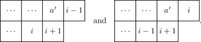
      Therefore, $T''_z=D_i(T''_y)$ and the desired result follows from Lemmas A.1 and A.3.

    • Alternatively suppose that $a'$ is not greater than every entry in row 2 of $T_y$. Then, we have $\textsf{frow}_y(a)>\textsf{frow}_y(c)=2$ and the second rows of $T'_y\leftarrow c$ and $T''_y$ are

      

      so $\textsf{ivalue}^y_{a}(3)=a''$. Similarly, we have $\textsf{frow}_z(c)=2$ and the second rows of $T'_z\leftarrow c$ and $T''_z$ appear as

      

      so $\textsf{ivalue}^z_{a}(3)=a''$. As a result, we have $i\prec _{T''_y}i-1 \prec _{T''_y}i+1$ and $T''_z=D_i(T''_y)$. Therefore, the desired result again follows from Lemmas A.1 and A.3.

  • ii. We could have $y=\cdots (b,i-1)(a,i)\cdots (i+1,c)\cdots$ and $z=\cdots (b,i-1)(a,i+1)\cdots (i,c)\cdots$ where $a<b<i-1<i+1<c$, so that y and z have arc diagrams

    

    In this case, denote the partial tableaux for y obtained just after inserting $(b,i-1)$, just after inserting (a, i), just before inserting $(i+1,c)$, and just after inserting $(i+1,c)$ by T, $T_y$, $T'_y$, and $T''_y$, respectively. Define $T_z$, $T'_z$, and $T''_z$ relative to z similarly. Then, $T_z$ is just $T_y$ after replacing i by $i+1$. We abbreviate by writing

    $$\begin{aligned} \textsf{frow}_y(b):=\textsf{frow}_{T\leftarrow b}\quad \text {and}\quad \textsf{frow}_y(a):=\textsf{frow}_{T_y\leftarrow a}. \end{aligned}$$

    Since $a<b$, we must have $\textsf{frow}_y(b)<\textsf{frow}_y(a)$ by Lemma A.2 and then $i\prec _{T'_y} i-1$. After the insertions $T'_y\xleftarrow {\hspace{0.5mm}\textsf{cB}\hspace{0.5mm}}(i+1,c)$ and $T'_z\xleftarrow {\hspace{0.5mm}\textsf{cB}\hspace{0.5mm}}(i,c)$, we get

    $$\begin{aligned} i\prec _{T''_y} i-1\prec _{T''_y} i+1 \quad \text {and}\quad T''_z=s_i(T''_y)=D_i(T''_y), \end{aligned}$$

    so the desired result follows from Lemmas A.1 and A.3.

  • iii. We could have $y=\cdots (a,i)\cdots (i-1,b)\cdots (i+1,c)\cdots$ and $z=\cdots (a,i+1)\cdots (i-1,b)\cdots (i,c)\cdots$ where $a<i-1<i+1<b<c$, so that

    

    Let $T_y$ denote the partial tableau for y obtained after inserting (a, i), let $T'_y$ be the partial tableau for y obtained after inserting $(i-1,b)$, let $T''_y$ be the partial tableau for y obtained before inserting $(i+1,c)$, and let $T'''_y$ be the partial tableau for y obtained after inserting $(i+1,c)$. Define $T_z$, $T'_z$, $T''_z$, and $T'''_z$ relative to z similarly. Then, $T'_z$ is just $T'_y$ after replacing i by $i+1$, and we have $i\prec _{T'_y} i-1$. Thus, by Lemma A.1, we have $i\prec _{T''_y} i-1$. Now, consider the insertion $T''_y\xleftarrow {\hspace{0.5mm}\textsf{cB}\hspace{0.5mm}}(i+1,c)$ and $T''_z\xleftarrow {\hspace{0.5mm}\textsf{cB}\hspace{0.5mm}}(i,c)$. Then, $i+1$ is in the first row of $T'''_y$, while i is in the first row of $T'''_z$, so

    $$\begin{aligned}i\prec _{T'''_y} i-1_{T'''_y}\prec i+1\quad \text {and}\quad T'''_z=s_i(T'''_y)=D_i(T'''_y).\end{aligned}$$

    Thus, the desired result follows from Lemmas A.1 and A.3.

  • iv. Finally, we could have $y=\cdots (i,a)\cdots (i-1,b)\cdots (i+1,c)\cdots$ and $z=\cdots (i+1,a)\cdots (i-1,b)\cdots (i,c)\cdots$ where $i+1<a<b<c$, so that

    

    In this case, the proof is similar to case iii after replacing (a, i) by (i, a).

• (3e) Assume $y(i-1)=i+1$ and $y(i)=a<i-1$. In this case, $y=\cdots (a,i)(i-1,i+1)\cdots$ and $z=\cdots (i-1,i)(a,i+1)\cdots$ have arc diagrams

  

  Let T denote the partial tableau for y obtained just before inserting (a, i). Then, let $T_y$ and $T'_y$ be the partial tableaux for y obtained after inserting (a, i) and $(i-1,i+1)$, respectively. Likewise, define $T_z$ and $T'_z$ to be the partial tableaux for z obtained after inserting $(i-1,i)$ and $(a,i+1)$, respectively. Then, write

  $$\begin{aligned} \textsf{ivalue}^y_a(k):= \textsf{ivalue}_{T\leftarrow a}(k) \quad \text {and}\quad \textsf{ivalue}^y_{i-1}(k):=\textsf{ivalue}_{T_y\leftarrow i-1}(k). \end{aligned}$$

  Also, write

  $$\begin{aligned} \textsf{frow}_y(a):=\textsf{frow}_{T\leftarrow a}\quad \text {and}\quad \textsf{frow}_y(i-1):=\textsf{frow}_{T_y\leftarrow i-1}. \end{aligned}$$

  There are now two cases, as we either have (I) $\textsf{frow}_y(a)=1$ or (II) $\textsf{frow}_y(a)=j>1$. In case (I), since $\textsf{frow}_y(a)=1$, the first two rows of $T'_y$ and $T'_z$ appear as

  

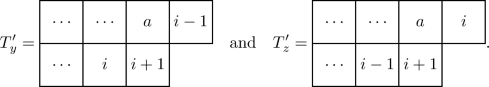
  Thus, we have $i\prec _{T'_y}i+1\prec _{T'_y}i-1$ and $T'_z=s_i(T'_y)$ and the desired result follows from Lemma A.3. Suppose instead that we are in case (II). If i is in the first row of $T_y$, then a and i are the last two elements in the first row of $T_y$. Thus, $T_y$ and $T_z$ appear as below, where we write $f=\textsf{frow}_y(a)$ and $a_j=\textsf{ivalue}^y_a(j)$ for $j<f$ (so $a=a_1$)

  

  After inserting $(i-1,i+1)$ into $T_y$ and $(a,i+1)=(a_1,i+1)$ into $T_z$, we get

  

  so we have

  $$\begin{aligned} i\prec _{T'_y}i-1\prec _{T'_y}i+1 \quad \text {and}\quad T'_z=s_{i-1}(T'_y)=D_i(T'_y). \end{aligned}$$

  If i is not in the first row of $T_y$, then $\textsf{frow}_y(a)>\textsf{frow}_y(i-1)$, so $\textrm{B}_{T\leftarrow a}\cap \textrm{B}_{T_y\leftarrow i-1}=\varnothing$. Thus, interchanging the order in which we insert the cycles involving a and $i-1$ does not change anything but the position of i and $i+1$. Consequently, we have

  $$\begin{aligned} i\prec _{T'_y}i-1\prec _{T'_y}i+1\quad \text {and}\quad T'_z=s_i(T'_y)=D_i(T'_y). \end{aligned}$$

  Either way, the desired result follows from Lemmas A.1 and A.3.

In all of these cases, we deduce that $P_{\textsf{cB}}(y) = D_i(P_{\textsf{cB}}(z))$ as needed. $\square$

Propositions A.5, A.7, and A.8 address the three cases in Theorem 2.13. By combining these results, the theorem follows.

References

R. Adin, A. Postnikov, and Y. Roichman, Combinatorial Gelfand models, J. Algebra 320 (2008), 1311–1325.
S. Assaf, Dual equivalence graphs I: A new paradigm for Schur positivity, Forum Math. Sigma, 3, Article e12 (2015).
J. S. Beissinger, Similar constructions for Young tableaux and involutions, and their application to shiftable tableaux, Discrete Math. 67 (1987), 149–163.
A. Björner and F. Brenti, Combinatorics of Coxeter groups, Graduate Texts in Mathematics 231 (2005), Springer, New York
P. Edelman and C. Greene, Balanced tableaux, Adv. Math. 63 (1987), no. 1, 42–99.
B. Elias and G. Williamson, The Hodge theory of Soergel bimodules, Ann. Math. 180 (2014), 1089–1136.
M. Haiman, Dual equivalence with applications, including a conjecture of Proctor, Discrete Math. 99 (1992), 79–113.
J. E. Humphreys, Reflection groups and Coxeter groups, Cambridge University Press, Cambridge, 1990.
D. Kazhdan and G. Lusztig, Representations of Coxeter groups and Hecke algebras, Invent. Math. 53 (1979), 165–184.
E. Marberg, Bar operators for quasiparabolic conjugacy classes in a Coxeter group, J. Algebra 453 (2016), 325–363.
E. Marberg and B. Pawlowski, Gröbner geometry for skew-symmetric matrix Schubert varieties, Adv. Math. 405 (2022), 108–488.
E. Marberg and Y. Zhang, Gelfand \(W\)-graphs for classical Weyl groups, J. Algebra 609 (2022), 292–336.
E. Marberg and Y. Zhang, Perfect models for finite Coxeter groups, J. Pure Appl. Algebra 227 (2023), 107303.
V. M. Nguyen, Type \(A\) admissible cells are Kazhdan–Lusztig, Algebr. Comb. 3 (2020) no. 1, 55–105.
J. Post, Combinatorics of arc diagrams, Ferrers fillings, Young tableaux and lattice paths, M.Sc. Thesis, Simon Fraser University (2009).
E. M. Rains and M. J. Vazirani, Deformations of permutation representations of Coxeter groups, J. Algebr. Comb. 37 (2013), 455–502.
A. Reifegerste, Permutation sign under the Robinson–Schensted–Knuth correspondence, Ann. Combin. 8 (2004), 103–112.
C. Schensted, Longest increasing and decreasing subsequences, Can. J. Math. 13 (1961), 179–191.
J. R. Stembridge, Admissible \(W\)-Graphs, Represent. Theory 12 (2008), 346–368.
Y. Zhang, Quasiparabolic sets and affine fixed-point-free involutions, J. Algebra 587 (2021), 522–554.
Acknowledgements
The authors are very grateful to Joel Lewis for helpful discussions which benefited this work, and for contributing the proof of Proposition 2.14.
Funding
Open access funding provided by Hong Kong University of Science and Technology. This work was partially supported by grant GRF 16306120 from the Hong Kong Research Grants Council and by grant 2023M741827 from the China Postdoctoral Science Foundation. The authors have no other relevant financial or non-financial interests to disclose.
Author information
Authors and Affiliations
Corresponding author
Additional information
Communicated by Nathan Williams.
Publisher's Note
Springer Nature remains neutral with regard to jurisdictional claims in published maps and institutional affiliations.