Structured Condition Number for a Certain Class of Functions of Non-commuting Matrices

Abstract

We investigate the structured condition number of a class of functions of two non-commuting matrices with some type of structure, in order to assess the sensitivity of structured perturbations in the input matrices. This might have interest in several practical applications, like the computation of the geometric mean of two symmetric positive definite matrices or the exp-log mean of two symplectic matrices. These two particular matrix functions deserve a particular study, as well as the matrix-matrix exponentiation. Algorithms for computing the structured condition number are proposed, but they are in general expensive. To round this issue, we derive lower and upper bounds for estimating the structured condition number. Results regarding the comparison between the structured and unstructured condition numbers for pairs of symmetric or skew-symmetric input matrices are provided. Several numerical experiments involving many structured matrices are carried out to compare the structured condition number with the bounds and also with the unstructured condition number.

1 Introduction

This paper deals with the class of functions of two non-commuting matrices introduced in [13, Sec. 3]. Such a class is constituted by functions whose expression is based on a combination of primary matrix functions and is revisited here by convenience. We refer the reader to [22, 25] for details about primary matrix functions. Throughout the text, ${\mathbb {K}}$ denotes either ${\mathbb {R}}$ or ${\mathbb {C}}$.

Definition 1

Let $A,B\in {\mathbb {K}}^{n\times n}$ and let the symbol $\circledast$ denote either a matrix sum or a matrix product, so that $A \circledast B$ means $A + B$ or AB. Assume that $\phi (z)$, ${\widetilde{\phi }}(z)$ and $\psi (z)$ are scalar valued complex functions such that $\phi (A)$, ${\widetilde{\phi }}(B)$ and $\psi \left( \phi (A)\circledast {\widetilde{\phi }}(B)\right)$ are primary matrix functions. We say that

$$\begin{aligned} \begin{array}{cccc} {{\varvec{f}}}:&{} {\mathbb {K}}^{n\times n}\times {\mathbb {K}}^{n\times n} &{} \longrightarrow &{} {\mathbb {K}}^{n\times n}\\ &{} (A,B) &{} \longmapsto &{} C=f(A,B) \end{array} \end{aligned}$$

belongs to the ${{\mathcal {P}}}_2$ class (${{\mathcal {P}}}$ from primary and 2 from two variables), if ${{\varvec{f}}}(A,B)$ can be written as a finite number of products and/or sums of functions of the form $\psi \left( \phi (A)\circledast {\widetilde{\phi }}(B)\right)$.

The class of functions ${{\mathcal {P}}}_2$ includes well-known functions depending on two non-commuting matrices. For instance, the matrix-matrix exponentiation [7], the Lie bracket [17], means of two matrices [4, 19, 26], matrix beta function [28], polynomials in A and B (particular cases of polynomials of two non-commuting variables, that is, linear combinations of products of powers of the variables), rational functions involving two non-commuting matrices, etc..

The definition we used (Definition 1) makes it easier to extend the Fréchet derivatives to functions that depend on two matrices. Such derivatives play a key role in the definition of condition numbers that allow us to measure the sensitivity of functions in the ${{\mathcal {P}}}_2$ class to perturbations of first order in the input matrices A and B.

In this work, we assume that A and B have a special structure, that is, they belong to either a certain automorphism group, a Lie algebra or a Jordan algebra associated with a given scalar product. In the numerical computation of ${{\varvec{f}}}(A,B)$, it is important to assess the sensitivity of ${{\varvec{f}}}$ to perturbations in A and B. If A is perturbed by an arbitrary matrix E and B is perturbed by another arbitrary matrix F, then the unstructured condition number provides a key tool to understand such a sensitivity. However, if the perturbations are structured, i.e., if A and $A+E$ (resp., B and $B+F$) have the same structure, then the unstructured condition number may be useless, especially if it has a large value. To deal with these cases, we need to define and estimate the structured condition number of a function in ${{\mathcal {P}}}_2$ to understand how structure preserving algorithms for computing ${{\varvec{f}}}(A,B)$ behave when implemented in finite precision environments. If the unstructured condition number is large while the structured one is small, this misleads us to think that the problem is ill conditioning when actually it is not. This makes clear the importance of investigating the structured condition number. As will be seen in Section 2.2, the structured condition number takes into account the structure of the matrices while the unstructured one does not.

There is a large literature devoted to study structured problems, including the computation of functions depending on a single structured matrix; see [22, Sec.14.1] and the large amount of the references therein. We recall here by convenience what is written at the beginning of Sec.14.1 of Higham’s book: “ In many applications the matrices that arise are structured and when structure is present it is natural to try to exploit it. The benefits to be gained include faster and more accurate algorithms and reduced storage, as well as more physically meaningful solutions in the presence of rounding and truncation errors.”

As far as we know, this paper is the first one dedicated to the investigation of the structured condition number of functions depending on two non-commuting structured matrices. We propose a definition to the structured condition number of a function ${{\varvec{f}}}$ in ${{\mathcal {P}}}_2$ that extends the definition considered in [6, 14] for primary matrix functions. It turns out that the computation of the exact structured condition number requires the orthogonalization of a set of vectors with dimension $n^2$, which is an expensive procedure. To overcome this issue, we derive upper and lower bounds on the structured condition number, that are relatively cheaper to compute than obtaining the exact structured condition number. Our general results are then applied to particular functions in ${{\mathcal {P}}}_2$, such as the geometric mean, the exp-log mean and the matrix-matrix exponentiation. By exploiting the properties of these functions and the structure of the matrices A and B, we design algorithms to compute the structured condition number. A set of numerical experiments is then carried out to understand whether the estimates given by the bounds are reliable and also to compare the structured condition number with the unstructured one.

If $M^TM=I,\ M^T=-M$, it is proved in [14] that the structured and the unstructured condition numbers of primary matrix functions coincide, whenever the input matrix is symmetric or belongs to a Lie algebra. A comparison between those two condition numbers is also investigated for functions in ${{\mathcal {P}}}_2$, when A and B are either symmetric or skew-symmetric. Unfortunately, their values may be different, in particular, for the matrix-matrix exponentiation function. However, the numerical examples suggest that they coincide for both the geometric and exp-log means in the special case of A and B being symmetric. When A and B are skew-symmetric, we will see that, in general, the structured and the unstructured condition numbers are distinct. A couple of interesting results relating those two condition numbers when the input matrices are symmetric or skew-symmetric are stated.

Let us now recall the definition of three functions in ${{\mathcal {P}}}_2$ whose structured condition number will be investigated in this work. The first one is the geometric mean function $A\# B$ of two Hermitian positive definite matrices A and B, which may be defined by [26]

$$\begin{aligned} A\# B:= A^{1/2} \left( A^{-1/2}BA^{-1/2}\right) ^{1/2} A^{1/2}, \end{aligned}$$

(1)

where $Y=X^{1/2}$ stands for the principal square root of the matrix X. Recall that, for any matrix X with no non-positive eigenvalues, the principal square root Y of X is the unique matrix having eigenvalues on the open right half plane such that $Y^2=X$. Using the properties of the principal matrix square root, namely the fact that $(S\,X\,S^{-1})^{1/2}=S\,X^{1/2}\,S^{-1}$, for any non-singular matrix S, it can be shown that

$$\begin{aligned} A\# B=A(A^{-1}B)^{1/2}=(AB^{-1})^{1/2}B=(BA^{-1})^{1/2}A=B(B^{-1}A)^{1/2}. \end{aligned}$$

(2)

We recall that $A\#B$ as defined in (1) is a geodesic in the cone of symmetric positive definite matrices, in the sense that it minimizes the Riemannian distance; see, for instance, [31, Sec.3].

Ando, Li and Mathias defined the k-geometric means (ALM-mean) of positive definite matrices in [4]. Similarly to the ALM-mean, a new geometric mean is defined in [9], with applications in elasticity experiments in physics [21]. The matrix geometric mean has also applications in electrical networks [33], image processing [15] and medical imaging [5]. Trapp [35] also gave a list of applications of the geometric mean in electrical engineering literature.

In this paper, we consider the extension of the geometric mean concept to other matrices A and B, and use the notation f(A, B) instead of $A\# B$, that is,

$$\begin{aligned} f(A,B):= A^{1/2} \left( A^{-1/2}BA^{-1/2}\right) ^{1/2} A^{1/2}, \end{aligned}$$

(3)

where A and $A^{-1/2}BA^{-1/2}$ are assumed to have no non-positive real eigenvalue. The identities in (2) also hold in this case. We recall that means of matrices that are not symmetric positive definite might be of interest in applications; see for instance [30] for means of rotation matrices.

The second one is the exp-log mean function, which arises in applications in optometry [16, 18, 19]. Another application occurs in the different version of Hellinger distance given in terms of the geometric mean and the exp-log mean [8]. Hellinger distance is used to measure the similarity distance between two probability distributions.

Assuming that A and B have no eigenvalues on the closed negative real axis, the exp-log mean function is defined by

$$\begin{aligned} g(A,B)=e^{0.5(\log A+\log B)} \end{aligned}$$

(4)

where $e^X$ and $\log X$ denote the matrix exponential and the principal matrix logarithm of X, respectively.

The last function in ${{\mathcal {P}}}_2$ to be addressed with special emphasis is the matrix-matrix exponentiation. If A has no eigenvalue on the closed negative real axis and if B is a square matrix, then $A^B$ is defined as

$$\begin{aligned} h(A,B)=e^{(\log A)B}. \end{aligned}$$

(5)

Von Neumann found a connection between quantum mechanics and thermodynamics in 1931 [7]. The entropy of a quantum system can be written as

$$\begin{aligned} S(A)=-\log (\det (A^A)) \end{aligned}$$

for a density matrix A. In [7, Sec.4], the authors explain how this new representation of the entropy can bring benefits. Von Neumann’s entropy is also used to deal with the entanglement between the multipartite systems [32] and to obtain entropy of a black hole [10].

The paper is organized as follows. In Sect. 2, we start by reviewing the structured condition number of a primary matrix function, where we assume that the input matrix has some particular structure. Then, in Sect. 2.2, we generalize the concept of structured condition number to functions in ${{\mathcal {P}}}_2$ and derive lower and upper bounds to its value. Algorithms for computing exactly or estimate the structured condition number are proposed as well. The particular case when the input matrices are symmetric or skew-symmetric is investigated in Sect. 2.3. Section 3 deals with three particular functions in ${{\mathcal {P}}}_2$, where we construct the Kronecker forms of their Fréchet derivatives. In Sect. 4, a set of numerical results is carried out to illustrate our results and to investigate the significance of the structured condition number for functions in ${{\mathcal {P}}}_2$. In particular, we compare the structured condition number with their bounds and with the unstructured condition number. In the final section, some concluding remarks are drawn.

2 Sensitivity Analysis

An important tool to assess the sensitivity of a function f to perturbations of first order in the input matrix A is the Fréchet derivative. We recall that the Fréchet derivative of a primary matrix function f at A is a linear mapping $L_f(A,E): {\mathbb {K}}^{n \times n}\rightarrow {\mathbb {K}}^{n \times n}$ such that $\, \Vert f(A+E)-f(A) -L_f(A,E)\Vert = o(\Vert E\Vert ) \,$ for all $E\in {\mathbb {K}}^{n \times n}$. Applying the $\text{ vec }$ operator to $L_f(A,E)$ gives $\, \text{ vec }(L_f(A,E))=K_f(A)\text{ vec }(E),\,$ where $K_f(A)\in {\mathbb {K}}^{n^2\times n^2}$ is called the Kronecker form of the Fréchet derivative, where $\text{ vec }(.)$ denotes the operator that stacks the columns of a matrix into one column vector. See [22] for more information on the Fréchet derivative. Provided that f is Fréchet differentiable at A, the absolute (unstructured) condition number of a primary matrix function f(A) is given by

$$\begin{aligned} \mathrm {\mathop {cond}}(f,A):= \lim _{\epsilon \rightarrow 0} \sup _{\Vert E\Vert \le \epsilon } \frac{\Vert f(A+E) - f(A) \Vert }{\epsilon }, \end{aligned}$$

where $\Vert \cdot \Vert$ stands for a given matrix norm. For a more comprehensive exploration of the theory of condition numbers, please see [34]. The unstructured condition number can be expressed in terms of the norm of the Fréchet derivative:

$$\begin{aligned} \mathrm {\mathop {cond}}(f,A) = \max _{E\ne 0} \frac{\Vert L_f(A,E)\Vert }{\Vert E\Vert }. \end{aligned}$$

If we specialize to the Frobenius norm we obtain the unstructured condition number via the Kronecker form of the Fréchet derivative:

$$\begin{aligned} \mathrm {\mathop {cond}}(f,A)= \max _{E\ne 0} \frac{\Vert L_f(A,E)\Vert _F}{\Vert E\Vert _F} =\max _{E\ne 0} \dfrac{\Vert \text{ vec }(L_f(A,E))\Vert _2}{\Vert \text{ vec }(E)\Vert _2} =\Vert K_f(A)\Vert _2, \end{aligned}$$

where we use the fact that for $A\in {\mathbb {K}}^{n \times n}$, $\Vert A\Vert _{F}=\Vert \text{ vec }(A)\Vert _{2}$, where $\Vert \cdot \Vert _2$ stands for the 2-norm. Let M be a given real non-singular matrix and consider the scalar product from ${\mathbb {K}}^n\times {\mathbb {K}}^n$ to ${\mathbb {K}}$: $(x,y)\mapsto \langle x,y\rangle _M$ defined by

$$\begin{aligned} \langle x,y\rangle _M =\left\{ \begin{array}{ll} x^TMy, &{} \text {for real or complex bilinear forms,}\\ x^*My, &{} \text {for sesquilinear forms,} \end{array}\right. \end{aligned}$$

where $x^*$ stands for the conjugate transpose of x. For any matrix $A\in {\mathbb {K}}^{n \times n}$, there exists a unique $A^{{\textstyle \star }} \in {\mathbb {K}}^{n \times n}$, called the adjoint of A with respect to $\langle .,.\rangle _M$, that is given by

$$\begin{aligned} A^{{\textstyle \star }}= \left\{ \begin{array}{ll} M^{-1}A^TM, &{} \text {for real or complex bilinear forms,}\\ M^{-1}A^*M, &{} \text {for sesquilinear forms.} \end{array}\right. \end{aligned}$$

There are three classes of structured matrices associated with $\langle .\,,.\rangle _M$: a Jordan algebra ${\mathbb {J}}_M$, a Lie algebra ${\mathbb {L}}_M$ and an automorphism group ${\mathbb {G}}_M$, which are defined by

$$\begin{aligned}{} & {} {\mathbb {J}}_M {:}= \{ A\in {\mathbb {K}}^{n \times n} \,\mid \,A^{\textstyle \star }=A\},\qquad {\mathbb {L}}_M {:}= \{ A\in {\mathbb {K}}^{n \times n} \,\mid \,A^{\textstyle \star }=-A\}, \\{} & {} {\mathbb {G}}_M{:}= \{ A\in {\mathbb {K}}^{n \times n} \,\mid \,A^{\textstyle \star }=A^{-1}\}. \end{aligned}$$

For convenience, our focus in this work is on real and complex bilinear forms, so sesquilinear forms will not be addressed. In Table 1, we give examples of the most common algebraic structures generated by bilinear forms. The following notation is used:

(6)

where $I_s$ is the identity matrix of order s. All the matrices M involved in Table 1 satisfy $M^TM=I$ and $M=\mu M^T$, with $\mu =\pm 1$.

Table 1 Special choice of M for the structured matrices in ${\mathbb {J}}_M$, ${\mathbb {L}}_M$ and ${\mathbb {G}}_M$

2.1 Structured Condition Number for f(A)

In this work we restrict the function f to real submanifolds of the $n^2$-dimensional real vector space ${\mathbb {R}}^{n \times n}$ or complex submanifolds of the $n^2$-dimensional complex vector space ${\mathbb {C}}^{n \times n}$ associated with real bilinear forms and complex bilinear forms contained in the domain of f. We first review the structured condition number of primary matrix functions [6, 14].

Definition 2

Let $f: {\mathcal {M}}\rightarrow {\mathcal {N}}$ be a ${\mathbb {K}}$-differentiable map between two smooth square matrix manifolds ${\mathcal {M}},\,{\mathcal {N}}\subseteq {\mathbb {K}}^{n \times n}$. Given $A \in {\mathcal {M}}$, assume that f(A) is a primary matrix function. Then the absolute structured condition number of f(A) is

$$\begin{aligned} \mathrm {\mathop {cond}}_{\text{ struc }}(f,A) =\lim _{\epsilon \rightarrow 0} \sup _{\Vert X-A\Vert \le \epsilon \atop X \in {\mathcal {M}}} \dfrac{\Vert f(X) - f(A) \Vert }{\epsilon }. \end{aligned}$$

The extra condition $X \in {\mathcal {M}}$ restricts the choice of the perturbation $X-A$ to a smaller set, and hence, by the definition of supremum, obviously we have

$$\begin{aligned} \mathrm {\mathop {cond}}_{\text{ struc }}(f,A) \le \mathrm {\mathop {cond}}(f,A). \end{aligned}$$

For a smooth manifold ${\mathcal {M}}\subseteq {\mathbb {K}}^{n \times n}$ the matrix $E\in {\mathbb {K}}^{n \times n}$ is called a tangent vector of ${\mathcal {M}}$ at $A\in {\mathcal {M}}$ if there is a smooth curve $\gamma :{\mathbb {K}}\rightarrow {\mathcal {M}}$ such that $\gamma (0)=A$, $\gamma ^\prime (0)=E$. The tangent space of ${\mathcal {M}}$ at A is given as

$$\begin{aligned} T_A{\mathcal {M}}:=\{E\in {\mathbb {K}}^{n \times n} \,\mid \,\exists \ \gamma :{\mathbb {K}}\rightarrow {\mathcal {M}} \text{ smooth } \text{ with } \gamma (0)=A\text{, } \gamma '(0)=E\}. \end{aligned}$$

If $f:{\mathcal {M}}\rightarrow {\mathcal {N}}$ is ${\mathbb {K}}$-differentiable then the differential of f at the point A is the map

$$\begin{aligned} df_A:T_A{\mathcal {M}}\rightarrow T_{f(A)}{\mathcal {N}}, \quad df_{A}(\gamma ^\prime (0))=(f\circ \gamma )^\prime (0). \end{aligned}$$

The case ${\mathcal {M}}\subseteq {\mathbb {C}}^{n \times n}$ with f being ${\mathbb {R}}$-Fréchet differentiable f will not be analysed here. It is possible to express the structured condition number by the differential of f at A, which is defined between the tangent spaces in the following way:

$$\begin{aligned} \Vert df_A\Vert := \max _{E \in T_A {\mathcal {M}}\atop E\ne 0} \dfrac{\Vert df_A(E)\Vert }{\Vert E\Vert }. \end{aligned}$$

In [6, Thm. 2.3], it is proved that $\mathrm {\mathop {cond}}_{\text{ struc }}(f,A)=\Vert df_A\Vert$.

Let the columns of U span the tangent space $T_A {\mathcal {M}}$ and let $p=\dim _{{\mathbb {K}}}T_A {\mathcal {M}}$. Then, for any $E\in T_A {\mathcal {M}}$, there exists $y\in {\mathbb {K}}^p$ such that $\text{ vec }(E)=Uy$. The structured condition number is obtained as

$$\begin{aligned} \mathrm {\mathop {cond}}_{\text{ struc }}(f,A)= & {} \max _{E \in T_A {\mathcal {M}}\atop E\ne 0} \dfrac{\Vert \text{ vec }(L_f(A,E))\Vert _2}{\Vert \text{ vec }(E)\Vert _2}\\= & {} \max _{y\in {\mathbb {K}}^p \atop y\ne 0} \dfrac{\Vert K_f(A)Uy\Vert _2}{\Vert Uy\Vert _2} \\= & {} \dfrac{\Vert K_f(A)UU^+Uy\Vert _2}{\Vert Uy\Vert _2} \\= & {} \Vert K_f(A)UU^+\Vert _2, \end{aligned}$$

where $U^+$ denotes the Moore-Penrose inverse of U. By using the property $\Vert U^+\Vert _2^{-1}\Vert y\Vert _2\le \Vert Uy\Vert _2\le \Vert U\Vert _2\Vert y\Vert _2$, we can obtain the following upper and the lower bounds:

$$\begin{aligned} \Vert K_f(A)U\Vert _2\Vert U\Vert _2^{-1}\le \mathrm {\mathop {cond}}_{\text{ struc }}(f,A)\le \Vert K_f(A)U\Vert _2\Vert U^+\Vert _2. \end{aligned}$$

(7)

If U has orthonormal columns then the upper and lower bounds coincide and

$$\begin{aligned} \mathrm {\mathop {cond}}_{\text{ struc }}(f,A)=\Vert K_f(A)U\Vert _2. \end{aligned}$$

2.2 Structured Condition Number for f(A, B)

Let ${\mathcal {M}}_1\subseteq {\mathbb {K}}^{n \times n}$ and ${\mathcal {M}}_2\subseteq {\mathbb {K}}^{n \times n}$ be smooth square matrix manifolds. Given the matrix function $f(A,B):{\mathcal {M}}_1\times {\mathcal {M}}_2\rightarrow {\mathcal {N}}$, the Fréchet derivative [13] is defined by

$$\begin{aligned} \Vert f(A+E,B+F)-f(A,B)-L_f(A,B;E,F) \Vert =o\left( \Vert (E,F)\Vert \right) . \end{aligned}$$

Assuming that f is Fréchet differentiable at (A, B), with respect to an induced norm, we obtain the unstructured condition number

$$\begin{aligned} \mathrm {\mathop {cond}}(f,(A,B)):=\max _{ (E,F)\ne 0} \dfrac{\Vert L_f(A,B;E,F)\Vert }{\Vert (E,F)\Vert }. \end{aligned}$$

We recall that the condition number gives an upper perturbation bound for small perturbations E and F:

$$\begin{aligned} \dfrac{\Vert f(A+E,B+F)-f(A,B)\Vert }{\Vert f(A,B)\Vert } \le \mathrm {\mathop {cond}}(f,(A,B))\dfrac{\Vert (E,F)\Vert }{\Vert f(A,B)\Vert }+o(\Vert (E,F)\Vert ). \end{aligned}$$

Applying the $\text{ vec }$ operator to the Fréchet derivative of f(A, B), gives

$$\begin{aligned} \text{ vec }(L_f(A,B;E,F))=K_f(A,B)\begin{bmatrix} \text{ vec }(E)\\ \text{ vec }(F) \end{bmatrix}, \end{aligned}$$

(8)

where $K_f(A,B)\in {\mathbb {K}}^{n^2\times 2n^2}$ is the Kronecker form of the Fréchet derivative and $\mathrm {\mathop {cond}}(f,(A,B))=\Vert K_f(A,B)\Vert _2$. For the structured condition number, we propose the following definition:

$$\begin{aligned} \mathrm {\mathop {cond}}_{\text{ struc }}(f,(A,B))=\lim _{\epsilon \rightarrow 0} \sup _{\Vert (X-A,Y-B)\Vert \le \epsilon \atop X \in {\mathcal {M}}_1,\, Y\in {\mathcal {M}}_2 } \dfrac{\Vert f(X,Y) - f(A,B) \Vert }{\epsilon }. \end{aligned}$$

(9)

The differential of f at the point (A, B) is defined between the tangent spaces $T_{(A,B)}\left( {\mathcal {M}}_1\times {\mathcal {M}}_2\right)$ and $T_{f(A,B)}{\mathcal {N}}$ [36]:

$$\begin{aligned} df_{(A,B)}: T_{(A,B)}\left( {\mathcal {M}}_1\times {\mathcal {M}}_2\right) \rightarrow T_{f(A,B)}{\mathcal {N}}, \end{aligned}$$

where we can write $T_{(A,B)}\left( {\mathcal {M}}_1\times {\mathcal {M}}_2\right) =T_A{\mathcal {M}}_1\times T_B{\mathcal {M}}_2$, which restricts the perturbation matrices to the corresponding tangent spaces, that is, $E \in T_A {\mathcal {M}}_1$ and $F \in T_B {\mathcal {M}}_2$.

Theorem 1

Let $f:\Omega _1\times \Omega _2\rightarrow \Omega$ be a map between the open subsets $\Omega _1\subset {\mathcal {M}}_1$, $\Omega _2\subset {\mathcal {M}}_2$ and $\Omega \subset {\mathcal {N}}$, where ${\mathcal {M}}_1$, ${\mathcal {M}}_2$ and ${\mathcal {N}}$ are smooth square matrix manifolds of ${\mathbb {K}}^{n \times n}$. Assuming that $f\in {{\mathcal {P}}}_2$, for any pair $(A,B)\in \Omega _1\times \Omega _2$, we have

$$\begin{aligned} \mathrm {\mathop {cond}}_{\text{ struc }}(f,(A,B))=\Vert df_{(A,B)}\Vert . \end{aligned}$$

Proof

Consider the curves $X(t)=A+tE$ with $X(0)=A$, $X(\epsilon )=X$, $X^\prime (0)=E$ and $Y(t)=B+tF$ with $Y(0)=B$, $Y(\epsilon )=Y$, $Y^\prime (0)=F$. For all t in a certain neighbourhood of 0, we assume that $X(t)\in \Omega _1$ and $Y(t)\in \Omega _2$. We can write the following: $f(X,Y)=f(A,B)+\epsilon \, df_{(A,B)}(E,F)+o(\epsilon ).$ From the definition of the structured condition number we obtain

$$\begin{aligned} \mathrm {\mathop {cond}}_{\text{ struc }}(f,(A,B))&= \lim _{\epsilon \rightarrow 0} \sup _{\Vert (X-A,Y-B)\Vert \le \epsilon \atop X \in \Omega _1,\, Y\in \Omega _2 } \dfrac{\Vert f(X,Y) - f(A,B) \Vert }{\epsilon } \\&= \lim _{\Vert (X-A,Y-B)\Vert \rightarrow 0} \sup _{ X \in \Omega _1 \atop Y\in \Omega _2 } \dfrac{\Vert f(X,Y) - f(A,B) \Vert }{\Vert (X-A,Y-B)\Vert } \\&= \lim _{\epsilon \rightarrow 0} \sup _{ E \in T_A\Omega _1\atop F\in T_B\Omega _2} \dfrac{\epsilon \Vert df_{(A,B)}(E,F)\Vert +o(\epsilon )}{\epsilon \Vert (E,F)\Vert +o(\epsilon )} \\&= \Vert df_{(A,B)}\Vert . \end{aligned}$$

$\square$

From the uniqueness of the differential and the Fréchet derivative we conclude that $df_{(A,B)}(E,F)=L_f(A,B;E,F).$ Hence, for $A\in {\mathcal {M}}_1$ and $B\in {\mathcal {M}}_2$, the structured condition number may be written in terms of the Fréchet derivative as

$$\begin{aligned} \mathrm {\mathop {cond}}_{\text{ struc }}(f,(A,B))=\max _{E \in T_A {\mathcal {M}}_1, \,\, F \in T_B {\mathcal {M}}_2 \atop (E,F)\ne 0} \dfrac{\Vert L_f(A,B;E,F)\Vert }{\Vert (E,F)\Vert }. \end{aligned}$$

With respect to the Frobenius norm, we have

$$\begin{aligned} \mathrm {\mathop {cond}}_{\text{ struc }}(f,(A,B))= & {} \max _{E \in T_A {\mathcal {M}}_1, \,\, F \in T_B {\mathcal {M}}_2 \atop (E,F)\ne 0} \dfrac{\Vert L_f(A,B;E,F)\Vert _F}{\Vert (E,F)\Vert _F}\\= & {} \max _{y_1\in {\mathbb {K}}^{p_1}, \,\, y_2\in {\mathbb {K}}^{p_2}\atop y_1\ne 0,\,\, y_2\ne 0}\dfrac{\Vert K_f(A,B)Uy\Vert _2}{\Vert Uy\Vert _2}\\= & {} \Vert K_f(A,B) U U^+\Vert _2. \end{aligned}$$

Here $U\in {\mathbb {K}}^{2n^2\times (p_1+p_2)}$, with $p_1=\dim _{{\mathbb {K}}}T_A {\mathcal {M}}_1$, $p_2=\dim _{{\mathbb {K}}}T_B {\mathcal {M}}_2$, and y are given as

$$\begin{aligned} U= \begin{bmatrix} U_1 &{}\quad 0 \\ 0 &{}\quad U_2\end{bmatrix}, \quad \quad y= \begin{bmatrix}y_1\\ y_2\end{bmatrix},\quad y_1\in {\mathbb {K}}^{p_1} \, \,\text {and} \, \, y_2\in {\mathbb {K}}^{p_2}, \end{aligned}$$

where the columns of $U_1\in {\mathbb {K}}^{n^2\times p_1}$ and $U_2\in {\mathbb {K}}^{n^2\times p_2}$ are the bases of $T_A{\mathcal {M}}_1$ and $T_B{\mathcal {M}}_2$, respectively. Substituting $\text{ vec }(E)=U_1y_1$ and $\text{ vec }(F)=U_2y_2$ in (8) gives

$$\begin{aligned} K_f(A,B)\begin{bmatrix} \text{ vec }(E)\\ \text{ vec }(F) \end{bmatrix}= K_f(A,B)\begin{bmatrix} U_1y_1\\ U_2y_2 \end{bmatrix}= K_f(A,B)\begin{bmatrix} U_1 &{} 0 \\ 0 &{} U_2\end{bmatrix}\begin{bmatrix} y_1\\ y_2 \end{bmatrix}. \end{aligned}$$

Hence, we obtain the following bounds which extend the ones given in (7) to $f\in {{\mathcal {P}}}_2$:

$$\begin{aligned} \Vert K_f(A,B)U\Vert _2\Vert U\Vert _2^{-1}\le \Vert K_f(A,B)UU^+\Vert _2\le \Vert K_f(A,B)U\Vert _2\Vert U^+\Vert _2. \end{aligned}$$

(10)

If U has orthonormal columns, then the structured condition number of f(A, B) can be computed by means of the Kronecker form of the Fréchet derivative:

$$\begin{aligned} \mathrm {\mathop {cond}}_{\text{ struc }}(f,(A,B))=\Vert K_f(A,B)U\Vert _2. \end{aligned}$$

However, if U does not have orthonormal columns, then

$$\begin{aligned} \mathrm {\mathop {cond}}_{\text{ struc }}(f,(A,B))\le \Vert K_f(A,B)U\Vert _2. \end{aligned}$$

Now we summarize the process of constructing the basis $U_1$ and $U_2$ of the tangent spaces $T_A{\mathcal {M}}_1$ and $T_B{\mathcal {M}}_2$, respectively, at the structured matrices A and B. For more details, see [6]. Let ${\mathbb {S}}_M$ represent either ${\mathcal {M}}_1$ or ${\mathcal {M}}_2$. For ${\mathbb {S}}_M\in \{{\mathbb {J}}_M,{\mathbb {L}}_M\}$, the basis of the tangent space of ${\mathbb {S}}_M$, which is ${\mathbb {S}}_M$ itself, can be given by

$$\begin{aligned} U_{{\mathbb {S}}_M}=(I_n\otimes M^{-1})D_{{\mathbb {S}}_M}, \end{aligned}$$

(11)

with

(12)

where $s=1$ if ${\mathbb {S}}_M={\mathbb {J}}_M$, $s=-1$ if ${\mathbb {S}}_M={\mathbb {L}}_M$ and ${\widetilde{D}}_{\mu s}\in {\mathbb {R}}^{n^2\times n(n-1)/2}$ is a matrix with columns

$$\begin{aligned} (e_{(i-1)n+j}+\mu s e_{(j-1)n+i})/\sqrt{2}, \quad 1\le i<j\le n, \end{aligned}$$

and $\check{I}\in {\mathbb {R}}^{n^2\times n}$ has the column vectors $e_{(i-1)n+i}$, $i=1,\dots ,n$. Here, $e_i$ denotes the $n^2\times 1$ vector with 1 in the i-position and zeros elsewhere and $\mu =\pm 1$ such that $M=\mu M^T$.

For real or complex bilinear forms, the basis of the tangent space to ${\mathbb {S}}_M\in \{{\mathbb {G}}_M\}$ at X is given by

$$\begin{aligned} U_{{\mathbb {G}}_M}=(I_n\otimes XM^{-1})D_{{\mathbb {L}}_M}. \end{aligned}$$

(13)

For example,

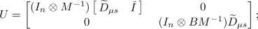
• if $A\in {\mathbb {J}}_M$ (suppose $\mu s=1$) and $B\in {\mathbb {G}}_M$ (suppose $\mu s=-1$), then the matrix U is built as

  

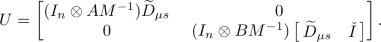
• if $A\in {\mathbb {G}}_M$ (suppose $\mu s=-1$) and $B\in {\mathbb {G}}_M$ (suppose $\mu s=1$), then the matrix U is given by

  

Provided that M is orthogonal and $M^T=\pm M$, for ${\mathbb {S}}_M\in \{{\mathbb {J}}_M,{\mathbb {L}}_M\}$, the columns of $U_{{\mathbb {S}}_M}$ given by (11) are ortohonormal so no orthonormalization process is required to compute the exact structured condition number. This is the case of all the Jordan and Lie algebras listed in Table 1. Recall that for ${\mathbb {S}}_M\in \{{\mathbb {J}}_M,{\mathbb {L}}_M\}$, $T_X {\mathbb {S}}_M={\mathbb {S}}_M$ since ${\mathbb {J}}_M$ and ${\mathbb {L}}_M$ are linear subspaces so they are flat smooth manifolds. However, if A or B are not orthogonal and belong to an automorphism group ${\mathbb {G}}_M$, the columns of $U_{{\mathbb {G}}_M}$ in (13) may not be orthonormal. Since $U_i$ has size $n^2\times p_i$, for some integer $p_i\le n^2$ ($i=1,2$), orthogonalizing its columns is in general an expensive procedure, requiring about $O(n^2p_i^2)$ operations (see [20, ch.5] for a description of the most used orthogonalization techniques). Our proposal to round this issue is to derive lower and upper bounds that are able to estimate the structured condition number in $O(pn^2)$ flops.

We now specify the bounds in (10) to four different cases, where the dependence on $\Vert U_i\Vert _2$ and $\Vert U^+_i\Vert _2$ ($i=1,2$) is avoided. For $\{{\mathbb {J}}_M,{\mathbb {L}}_M\}$ classes, we use the following inequalities

$$\begin{aligned} \Vert U^+\Vert _2&= \max \{\Vert U^+_1\Vert _2,\Vert U^+_2\Vert _2\}\le \max \{\Vert M_1\Vert _2,\Vert M_2\Vert _2\} \\ \Vert U\Vert _2&= \max \{\Vert U_1\Vert _2,\Vert U_2\Vert _2\} \le \max \{\Vert M^{-1}_1\Vert _2,\Vert M^{-1}_2\Vert _2\}. \end{aligned}$$

Here $M_1$ and $M_2$ are the real non-singular matrices involved in the scalar products defining ${\mathcal {M}}_1$ and ${\mathcal {M}}_2$, respectively, which are chosen from Eq. (6), according to the structure of A and B. For the $\{{\mathbb {G}}_M\}$ class, we have the inequalities

$$\begin{aligned} \Vert U_1\Vert _2&\le \Vert M^{-1}_1\Vert _2\Vert A\Vert _2 \quad \text {and}\quad \Vert U_1^+\Vert _2 \le \Vert D^T_{{\mathbb {L}}_{M_1}}(I_n\otimes A^TM_1)\Vert _2\le \Vert A\Vert _2\Vert M_1\Vert _2 \\ \Vert U_2\Vert _2&\le \Vert M^{-1}_2\Vert _2\Vert B\Vert _2 \quad \text {and}\quad \Vert U_2^+\Vert _2 \le \Vert D^T_{{\mathbb {L}}_{M_2}}(I_n\otimes B^TM_2)\Vert _2\le \Vert B\Vert _2\Vert M_2\Vert _2. \end{aligned}$$

Let us denote ${\hat{\kappa }}:=\mathrm {\mathop {cond}}_{\text{ struc }}(f,(A,B))$. So, for each class, the upper bounds are given as:

• (i) ${\mathcal {M}}_i, (i=1,2)$ is a Jordan or Lie algebra:

  $$\begin{aligned} \dfrac{\Vert K_f(A,B)U\Vert _2}{\max \{\Vert M_1\Vert _2,\Vert M_2\Vert _2\}} \le {\hat{\kappa }}\le \Vert K_f(A,B)U\Vert _2\max \{\Vert M_1\Vert _2,\Vert M_2\Vert _2\}. \end{aligned}$$

  (14)

• (ii) ${\mathcal {M}}_1$ and ${\mathcal {M}}_2$ are automorphism groups:

  $$\begin{aligned}{} & {} \dfrac{\Vert K_f(A,B)U\Vert _2}{\max \{\Vert A\Vert _2\Vert M_1\Vert _2,\Vert B\Vert _2\Vert M_2\Vert _2\}} \nonumber \\{} & {} \quad \le {\hat{\kappa }}\le \Vert K_f(A,B)U\Vert _2\times \max \{\Vert A\Vert _2\Vert M_1\Vert _2,\Vert B\Vert _2\Vert M_2\Vert _2\}. \end{aligned}$$

  (15)

• (iii) ${\mathcal {M}}_1$ is an automorphism group and ${\mathcal {M}}_2$ is a Jordan or Lie algebra:

  $$\begin{aligned} \dfrac{\Vert K_f(A,B)U\Vert _2}{\max \{\Vert A\Vert _2\Vert M_1\Vert _2,\Vert M_2\Vert _2\}} \le {\hat{\kappa }}\le \Vert K_f(A,B)U\Vert _2\max \{\Vert A\Vert _2\Vert M_1\Vert _2,\Vert M_2\Vert _2\}.\nonumber \\ \end{aligned}$$

  (16)

• (iv) ${\mathcal {M}}_1$ is a Jordan or Lie algebra and ${\mathcal {M}}_2$ is an automorphism group:

  $$\begin{aligned} \dfrac{\Vert K_f(A,B)U\Vert _2}{\max \{\Vert M_1\Vert _2,\Vert B\Vert _2\Vert M_2\Vert _2\}} \le {\hat{\kappa }}\le \Vert K_f(A,B)U\Vert _2\max \{\Vert M_1\Vert _2,\Vert B\Vert _2\Vert M_2\Vert _2\}.\nonumber \\ \end{aligned}$$

  (17)

Let us now assume that $M_1$ and $M_2$ are orthogonal and that $(A,B)\in {\mathbb {G}}_{M_1}\times {\mathbb {G}}_{M_2}$. Excepting the particular case $M_1=M_2=I$, in general there is no orthonormal basis U available to ${\mathbb {G}}_{M_1}\times {\mathbb {G}}_{M_2}$ and so we must resort to the bounds (15) to get an estimate of the structured condition number. In the next lines, we will derive an inequality that give some clues on how the condition number of the matrices A and B with respect to the Frobenius norm, $\kappa _F(A)=\Vert A\Vert _F\Vert A^{-1}\Vert _F$ and $\kappa _F(B)=\Vert B\Vert _F\Vert B^{-1}\Vert _F$, influence the quality of the estimate of the relative structured condition number ${\hat{\kappa }}{\Vert (A,B)\Vert _F}/{\Vert f(A,B)\Vert _F}$ provided by ${\Vert K_f(A,B)U\Vert _2}/{\Vert f(A,B)\Vert _F}$.

Since

$$\begin{aligned} \max \{\Vert A\Vert _2,\Vert B\Vert _2\}=\Vert \mathrm {\mathop {diag}}(A,B)\Vert _2\le \Vert \mathrm {\mathop {diag}}(A,B)\Vert _F=\Vert (A,B)\Vert _F, \end{aligned}$$

(15) yields

$$\begin{aligned} \dfrac{\Vert K_f(A,B)U\Vert _2}{\Vert (A,B)\Vert _F} \le {\hat{\kappa }}\le \Vert K_f(A,B)U\Vert _2\Vert (A,B)\Vert _F, \end{aligned}$$

and hence

$$\begin{aligned} \dfrac{\Vert K_f(A,B)U\Vert _2}{\Vert f(A,B)\Vert _F} \le {\hat{\kappa }}\dfrac{\Vert (A,B)\Vert _F}{\Vert f(A,B)\Vert _F} \le \dfrac{\Vert K_f(A,B)U\Vert _2}{\Vert f(A,B)\Vert _F}\Vert (A,B)\Vert ^2_F. \end{aligned}$$

Attending that $\Vert A^{-1}\Vert _F=\Vert A\Vert _F$ and $\Vert B^{-1}\Vert _F=\Vert B\Vert _F$ hold (recall that for any $X\in {\mathbb {G}}_M$, with M orthogonal, $X^{-1}=M^TX^TM$ implies that $\Vert X^{-1}\Vert _F=\Vert X\Vert _F$) so that $\Vert (A,B)\Vert ^2_F=\kappa _F(A)+\kappa _F(B)$, we arrive at

$$\begin{aligned} \dfrac{\Vert K_f(A,B)U\Vert _2}{\Vert f(A,B)\Vert _F} \le {\hat{\kappa }}\dfrac{\Vert (A,B)\Vert _F}{\Vert f(A,B)\Vert _F} \le (\kappa _F(A)+\kappa _F(B))\dfrac{\Vert K_f(A,B)U\Vert _2}{\Vert f(A,B)\Vert _F}.\nonumber \\ \end{aligned}$$

(18)

Inequality (18) shows in particular that if A or B are well-conditioned, so $\kappa _F(A)+\kappa _F(B)\approx 2$, then ${\Vert K_f(A,B)U\Vert _2}/{\Vert f(A,B)\Vert _F}$ provides an acceptable estimate to the relative structured condition number. The quality of the bound estimations according to the value of $\max \{\kappa _F(A),\kappa _F(B)\}$ will be discussed in Sect. 4.

In the two next algorithms, we address the computation of $\kappa :=\Vert K_f(A,B) U\Vert _2$, which corresponds to the structured condition number if U has orthonormal columns or to an upper bound if not. Algorithm 1 can be viewed as an extension of [6, Alg. 2.6] to the functions in the class ${{\mathcal {P}}}_2$, and, provided that U has orthonormal columns and that $L_f(A,B;E,F)$ can be computed exactly, it gives the exact structured condition number.

Algorithm 1

Let $f(A,B):{\mathcal {M}}_1\times {\mathcal {M}}_2\rightarrow {\mathcal {N}}$, where ${\mathcal {M}}_1$, ${\mathcal {M}}_2$ are smooth manifolds of ${\mathbb {K}}^{n\times n}$ and let $U_1$ and $U_2$ be bases of the tangent spaces $T_A{\mathcal {M}}_1$ and $T_B{\mathcal {M}}_2$, respectively. Assume that for any $E\in T_A{\mathcal {M}}_1$, $\text{ vec }(E)=U_1y_1$ for some $y_1\in {\mathbb {K}}^{p_1}$ and $F\in T_B{\mathcal {M}}_2$, $\text{ vec }(F)=U_2y_2$ for some $y_2\in {\mathbb {K}}^{p_2}$. Provided that an algorithm for evaluating the Fréchet derivative $L_f(A,B;E,F)$ is available, this algorithm computes $\kappa =\Vert K_f(A,B)U\Vert _2$, where $U= \mathrm {\mathop {diag}}(U_1,U_2)$.

In Step 3 (resp., Step 7), $\text{ vec }(E_i) = U_1e_i$ and $\text{ vec }(F_i) = U_2e_i$, where $e_i$ denotes the $p_1\times 1$ (resp., $p_2\times 1$) vector with 1 in the i-th position and zeros elsewhere.

Since Algorithm 1 is in general computationally expensive (about $O(p^2n^2+pn^3)$ flops, where constructing X costs $O(pn^3)$ flops and computing its 2-norm costs $O(p^2n^2)$ flops if f(A, B) and $L_f(A,B;E,F)$ can be computed in $O(n^3)$ flops), we can alternatively estimate the structured condition number by a cheaper method, like the following one, which is based on the power method which requires only $O(kpn^2)$ flops, where k is the number of iterations. To estimate $\Vert K_f(A,B)U\Vert _2$ by the power method, one needs to use the adjoint operator $L_f^\star (A,B;W)$, which satisfies the property

$$\begin{aligned} \text{ vec }\left( L_f^\star (A,B;W) \right) =K^*_f(A,B)\text{ vec }(W); \end{aligned}$$

(19)

see [23, Lem. 6.1] and also [13, Sec. 6].

Algorithm 2

With the same notation and conditions of Algorithm 1, this algorithm uses the power method to compute $\gamma$ such that $\gamma \le \Vert K_f(A,B)U\Vert _2$.

Algorithms 1 and 2 do not require the orthogonalization process for U. If U is orthonormal, Algorithm 1 gives the exact structured condition number while Algorithm 2 provides an estimate. Note however that the former algorithm is more expensive than the latter. If U does not have orthonormal columns, instead of orthonormalizing U, which is in general expensive, we may alternatively use the bound (10) or its specifications (14)–(17). The computation of the value $\Vert K_f(A,B)U\Vert _2$ involved in those bounds can be carried out by means of $O(kpn^2)$ flops, if estimated by Algorithm  2. Here k is the number of iterations required in the power method. In some cases, we may exploit the structure of $U_1$ and $U_2$ in line 3 of Algorithm 1 to reduce the cost.

In Algorithms 1 and 2 we need to compute the Fréchet derivative in the given directions. Depending on the way the Fréchet derivatives are evaluated (different functions require usually distinct procedures), these two algorithms can be adapted to particular functions belonging to the class ${{{\mathcal {P}}}}_2$. In particular, specifications of those algorithm to the geometric mean, exp-log mean and matrix-matrix exponentiation will be included in Sect. 3.

2.3 A and B are Either Symmetric or Skew-Symmetric

In this section, we investigate the structured condition number of a given function $f(A,B)\in {{\mathcal {P}}}_2$, in the particular case when A and B are both either symmetric or skew-symmetric matrices. Thus, we are assuming that $M=I$ and that either $A,B\in {\mathbb {J}}_I$ or $A,B\in {\mathbb {L}}_I$. This issue might be of interest for some functions involving structured matrices, like, for instance, the geometric mean of two symmetric positive definite matrices or the exponential of a sum of skew-symmetric matrices.

The results derived below involve the well-known commutation matrix $\Pi$ of order $\ell ^2$, which is the unique matrix that satisfies $\Pi \,\text{ vec }(X)=\text{ vec }(X^T)$, for any matrix X of order $\ell$ [29, Sec.9.2]. $\Pi$ is symmetric and orthogonal, with spectrum $\{-1,\,1\}$, where the eigenvalue $(-1)^i$ has multiplicity $n_i=\frac{1}{2}n(n+(-1)^i)$, $i=1,2$. Note that $n_1+n_2=n^2.$ Hence, there is a real orthogonal matrix Q such that

$$\begin{aligned} \Pi =Q\,\mathrm {\mathop {diag}}(-I_{n_1},I_{n_2})\,Q^T. \end{aligned}$$

(20)

Let us now consider the matrices

$$\begin{aligned} {\widetilde{U}}_i:=\frac{1}{2}\left( I_{n^2}+(-1)^i\,\Pi \right) , \end{aligned}$$

(21)

where $i=1,2$. Both matrices ${\widetilde{U}}_1$ and ${\widetilde{U}}_2$ are symmetric, idempotent and diagonalizable with eigenvalues 0 and 1. Moreover, if Q is the orthogonal matrix considered in (20), we have

$$\begin{aligned} {\widetilde{U}}_1= & {} Q\,\mathrm {\mathop {diag}}(I_{n_1},0_{n_2})\,Q^T, \\ {\widetilde{U}}_2= & {} Q\,\mathrm {\mathop {diag}}(0_{n_1},I_{n_2})\,Q^T. \end{aligned}$$

Lemma 1

Let $M=I$, and assume that $D_{{\mathbb {J}}_I}$ and $D_{{\mathbb {L}}_I}$ are matrices defined as in (12) and that $U_{{\mathbb {J}}_I}$ and $U_{{\mathbb {L}}_I}$ are defined as in (11). Then, both $U_{{\mathbb {J}}_I}=D_{{\mathbb {J}}_I}$ and $U_{{\mathbb {L}}_I}=D_{{\mathbb {L}}_I}$ have orthonormal columns, that is, $U_{{\mathbb {J}}_I}^T U_{{\mathbb {J}}_I}=I$ and $U_{{\mathbb {L}}_I}^T U_{{\mathbb {L}}_I}=I$. Moreover, $U_{{\mathbb {J}}_I}\,U_{{\mathbb {J}}_I}^T={\widetilde{U}}_2$ and $U_{{\mathbb {L}}_I} U_{{\mathbb {L}}_I}^T={\widetilde{U}}_1$, where ${\widetilde{U}}_i$ $(i=1,2)$ are given in (21).

Proof

The results follow from the way as the matrices $U_{{\mathbb {J}}_I}$ and $U_{{\mathbb {L}}_I}$ are defined. Check (11). $\square$

In [14, Sec.4], it is proven that, if A is symmetric or skew-symmetric, then the structured and the unstructured condition numbers of f(A) coincide. The proof is mainly based on the fact that the Kronecker form $K_f(A)$ is symmetric and commutes with the commutation matrix $\Pi$. Unfortunately, these results cannot be extended to functions $f(A,B)\in {{\mathcal {P}}}_2$. Indeed, if A and B are either both symmetric or skew-symmetric, the Kronecker form of the Fréchet derivative $K_f(A,B)=[K_1\ K_2]\in {\mathbb {K}}^{n^2\times 2n^2}$ is a non-square matrix, with $K_1$ and $K_2$ being in general non-symmetric. Moreover, $K_1$ and $K_2$ do not commute in general with $\Pi$ and $\mathrm {\mathop {cond}}(f,(A,B))$ and $\mathrm {\mathop {cond}}_{\text{ struc }}(f,(A,B))$ may not coincide. The connections we have found between these two condition numbers are stated in the following theorem. Before that, it is worth to recall that $U_{{\mathbb {J}}_I}$, $U_{{\mathbb {L}}_I}$, $\Pi$ and Q are real matrices, while $K_f(A,B)$ may be non-real if A or B have non-real entries.

Theorem 2

Let $A, B\in {\mathbb {K}}^{n\times n}$ be either both symmetric or skew-symmetric matrices such that $f(A,B)\in {{\mathcal {P}}}_2$ and let $S:=K_1K_1^*+K_2K_2^*$, where $K_1$ and $K_2$ are square matrices of order $n^2$ such that $K_f(A,B)=\left[ K_1\ K_2\right]$. Assume in addition that $K_1$ and $K_2$ commute with the commutation matrix $\Pi$.

• (i) $Q^T\,S\,Q=\mathrm {\mathop {diag}}\left( S_1,\,S_2\right)$, where Q is the orthogonal matrix in (20) and, for $i=1,2$, $S_i$ is a Hermitian matrix of order $n_i=\frac{1}{2}n(n+(-1)^i)$.

• (ii) If A and B are symmetric, then $\mathrm {\mathop {cond}}_{\text{ struc }}(f,(A,B))=\Vert S_2\Vert _2^{1/2}$ and

  $$\begin{aligned} \mathrm {\mathop {cond}}(f,(A,B))=\max \left\{ \Vert S_1\Vert _2^{1/2},\,\mathrm {\mathop {cond}}_{\text{ struc }}(f,(A,B)) \right\} . \end{aligned}$$

  (22)

• (iii) If A and B are skew-symmetric, then $\mathrm {\mathop {cond}}_{\text{ struc }}(f,(A,B))=\Vert S_1\Vert _2^{1/2}$ and

  $$\begin{aligned} \mathrm {\mathop {cond}}(f,(A,B))=\max \left\{ \mathrm {\mathop {cond}}_{\text{ struc }}(f,(A,B)),\, \Vert S_2\Vert _2^{1/2}\,\right\} . \end{aligned}$$

  (23)

Proof

To ease the notation, let $K:=K_f(A,B)=[K_1\ K_2]\in {\mathbb {K}}^{n^2\times 2n^2}$.

• (i) Let us consider the orthonormal basis $U_{{\mathbb {J}}_I}$ for ${\mathbb {J}}_I$, as defined in (11). Since $K_1$ and $K_2$ commute with $\Pi$, it is easy to show that $S=K_1K_1^*+K_2K_2^*$ commutes with ${\widetilde{U}}_2=\frac{1}{2}\left( I_{n^2}+\,\Pi \right)$. Because S is Hermitian, there exists R unitary and D diagonal with real entries, such that $S=R\,D\,R^*$. Let $V:=R^*Q$, where Q is the orthogonal matrix of (20). Hence

  $$\begin{aligned}{} & {} S\,{\widetilde{U}}_2 ={\widetilde{U}}_2\, S\\{} & {} \quad \iff R\,D\,R^*Q\,\mathrm {\mathop {diag}}(0_{n_1},I_{n_2})Q^T = Q\,\mathrm {\mathop {diag}}(0_{n_1},I_{n_2})\,Q^T R\,D\,R^*\\{} & {} \quad \iff V^*DV\,\mathrm {\mathop {diag}}(0_{n_1},I_{n_2})=\mathrm {\mathop {diag}}(0_{n_1},I_{n_2}) V^*DV, \end{aligned}$$

  which means that $V^*DV$ commutes with $\mathrm {\mathop {diag}}(0_{n_1},I_{n_2})$. If we denote $G:=V^*DV$ and partition it conformally with $\mathrm {\mathop {diag}}(0_{n_1},I_{n_2})$,

  $$\begin{aligned} G=\left[ \begin{array}{cc} G_1 &{} G_2 \\ G_3 &{} G_4 \end{array}\right] , \end{aligned}$$

  then

  $$\begin{aligned} \mathrm {\mathop {diag}}(0_{n_1},I_{n_2})\, G = G\,\mathrm {\mathop {diag}}(0_{n_1},I_{n_2}) \end{aligned}$$

  implies that $G_1$ and $G_4$ are Hermitian matrices of orders, respectively, $n_1$ and $n_2$, and $G_2$ and $G_3$ are zero matrices. Therefore,

  $$\begin{aligned}{} & {} V^*DV=\mathrm {\mathop {diag}}(G_1,\,G_4)\\{} & {} \quad \iff Q^TRDR^*Q =\mathrm {\mathop {diag}}(G_1,\,G_4)\\{} & {} \quad \iff Q^TS Q =\mathrm {\mathop {diag}}(G_1,\,G_4), \end{aligned}$$

  and the result follows by letting $S_1:=G_1$ and $S_2:=G_4$.

• (ii) For any matrix $X\in {\mathbb {K}}^{n\times n}$, it is known that $\Vert X\Vert _2^2=\Vert XX^*\Vert _2=\Vert X^*X\Vert _2$. Denoting $U:=\mathrm {\mathop {diag}}\left( U_{{\mathbb {J}}_I},\,U_{{\mathbb {J}}_I}\right)$, we have:

  $$\begin{aligned} \mathrm {\mathop {cond}}_{\text{ struc }}(f,(A,B))= & {} \Vert K\,U\Vert _2 \\= & {} \Vert (K\,U)^*\Vert _2 \\= & {} \left\| KU(KU)^*\right\| _2^{1/2} \\= & {} \left\| {\widetilde{U}}_2 S\right\| _2^{1/2} \\= & {} \left\| Q\,\mathrm {\mathop {diag}}(0_{n_1},I_{n_2})\,Q^T Q\,\mathrm {\mathop {diag}}(S_1,S_2)\,Q^T\right\| _2^{1/2} \\= & {} \left\| \mathrm {\mathop {diag}}(0_{n_1},S_2)\right\| _2^{1/2} \\= & {} \Vert S_2\Vert _2^{1/2}, \end{aligned}$$

  which proves the first part of the claim (ii). The equality (22) holds, because

  $$\begin{aligned} \mathrm {\mathop {cond}}(f,(A,B))= & {} \Vert K\Vert _2 \\= & {} \Vert K^*\Vert _2 \\= & {} \left\| KK^*\right\| _2^{1/2}\\= & {} \left\| \mathrm {\mathop {diag}}(S_1,\,S_2)\right\| _2^{1/2}\\= & {} \max \left\{ \Vert S_1\Vert _2^{1/2},\ \Vert S_2\Vert _2^{1/2} \right\} . \end{aligned}$$

• (iii) Similar to the proof of (ii). $\square$

If A and B are symmetric, it will be shown in Sect. 3 that both the matrix geometric mean and the exp-log mean satisfy the conditions of Theorem 2, namely $K_1$ and $K_2$ commute with $\Pi$. Hence, for these two functions we can ensure that the structured and unstructured condition numbers can be related by (22). Surprisingly, in all the experiments we have carried out with the matrix geometric and the exp-log means of randomized symmetric matrices, we have noticed an equality between those two condition numbers. Although we were not able to provide a theoretical support for this fact, a possible explanation may lie on the fact that the order of $S_2$, which is equal to $n_2=\frac{1}{2}n(n+1)$, is larger than the order of $S_1$ ($n_1=\frac{1}{2}n(n-1)$) which makes more probable that the largest singular value of S comes from $S_2$ instead of $S_1$. In contrast, no pair of skew-symmetric matrices A and B was found to illustrate a possible equality between the unstructured and the structured condition numbers.

In the case of the matrix-matrix exponentiation, in general the matrices $K_1$ and $K_2$ do not commute with $\Pi$, even in the particular case when A and B are commuting matrices and symmetric. Hence, the conditions of Theorem 2 are not satisfied and equality (22) may not be valid.

3 Some Important Functions in the Class ${{\mathcal {P}}}_2$

3.1 Matrix Geometric Mean

In this section, we will assume that f(A, B) stands for the geometric mean defined in (3).

Lemma 2

Let M be real non-singular and let $A, B\in {\mathbb {G}}_M$ (resp., ${\mathbb {J}}_M)$ such that A and $A^{-1/2}BA^{-1/2}$ have no non-positive eigenvalue. Then $f(A,B)\in {\mathbb {G}}_M$ (resp., ${\mathbb {J}}_M)$.

Proof

The (principal) matrix square root and the matrix inverse preserve automorphism groups [24]. Since ${\mathbb {G}}_M$ is closed under multiplications, the geometric mean preserves the automorphism group structure. To show that $A, B\in {\mathbb {J}}_M$ implies $f(A,B)\in {\mathbb {J}}_M$, we just need to carry out a few calculations and pay attention to the identities (2). $\square$

From Lemma 2, we can say, in particular, that if A and B are orthogonal (resp., symplectic, symmetric) matrices satisfying the above mentioned spectral restrictions, then f(A, B) is orthogonal (resp., symplectic, symmetric).

The Kronecker form of f(A, B) is given in the next lemma.

Lemma 3

Assume that A and $A^{-1/2}BA^{-1/2}$ have no non-positive eigenvalue. The Kronecker form of the Fréchet derivative of the matrix geometric mean function f(A, B) is given by

$$\begin{aligned} K_f(A,B)=\begin{bmatrix} (I\otimes Z+Y^T\otimes I)^{-1}\ {}&\ (I\otimes Z^{-1}+Y^{-T}\otimes I)^{-1} \end{bmatrix} \end{aligned}$$

(24)

where $Z=(AB^{-1})^{1/2}$ and $Y=(B^{-1}A)^{1/2}$.

Proof

The proof is omitted because it is somewhat similar to the one given in [26, Thm. 3.1], with the difference that here A and B may not be symmetric positive definite. $\square$

Algorithms 1 and 2 presented in Sect. 2.2 are now particularized for the geometric mean function.

Algorithm 3

Assume that $A\in {\mathcal {M}}_1$ and $B\in {\mathcal {M}}_2$, where ${\mathcal {M}}_1$, ${\mathcal {M}}_2$ are smooth matrix manifolds of ${\mathbb {K}}^{n\times n}$, are given. For any $E\in T_A{\mathcal {M}}_1$, with $\text{ vec }(E)=U_1y_1$ for some $y_1\in {\mathbb {K}}^{p_1}$ and $F\in T_B{\mathcal {M}}_2$, with $\text{ vec }(F)=U_2y_2$ for some $y_2\in {\mathbb {K}}^{p_2}$, this algorithm computes $\kappa =\Vert K_f(A,B)U\Vert _2$ $(U= \textrm{diag}(U_1,U_2))$ for the matrix geometric mean.

For the matrix geometric mean, the adjoint operator (19) is now given by

$$\begin{aligned} \text{ vec }\left( L_f^\star (A,B;W) \right) = \begin{bmatrix} (I\otimes Z^{*}+Y\otimes I)^{-1}\text{ vec }(W) \\ (I\otimes Z^{-*}+Y^{-1}\otimes I)^{-1}\text{ vec }(W) \end{bmatrix}. \end{aligned}$$

The following algorithm is employing the power method to estimate the structured condition number of geometric mean.

Algorithm 4

Given the same function and matrices as in Algorithm 3, this algorithm uses the power method to compute $\gamma$ such that $\gamma \le \Vert K_f(A,B)U\Vert _2$.

3.2 The Exp-Log Mean

We now return to the exp-log mean function g(A, B) defined in (4), which is written here for convenience: $g(A,B)=\exp (0.5(\log A+\log B))$.

Lemma 4

Let M be non-singular and let A and B have no eigenvalues on the closed negative real axis. If $A, B\in {\mathbb {G}}_M$ (resp., ${\mathbb {J}}_M$), then $g(A,B)\in {\mathbb {G}}_M$ (resp., ${\mathbb {J}}_M$).

Proof

The proof is mainly based on the fact that for any $X\in {\mathbb {G}}_M$ with no non-positive eigenvalue, $\log (X)\in {\mathbb {L}}_M$, while $e^Y\in {\mathbb {G}}_M$, for any $Y\in {\mathbb {L}}_M$. For more details see [12]. $\square$

Lemma 4 implies, in particular, that the exp-log mean of orthogonal (resp., symplectic) matrices is also orthogonal (resp., symplectic).

Lemma 5

Let A and B have no eigenvalues on the closed negative real axis. The Fréchet derivative of the exp-log mean of g at (A, B) in the direction of (E, F) is given by

$$\begin{aligned} L_g(A,B;E,F)=L_{\exp }\Big ( 0.5(\log A+\log B);\,0.5(L_{\log }(A,E)+L_{\log }(B,F))\Big ), \end{aligned}$$

where $L_{\exp }$ and $L_{\log }$ represent the Fréchet derivatives of the matrix exponential and the principal logarithm, respectively.

Proof

Using [13, Thm. 4.1], we have

$$\begin{aligned} g\left( \begin{bmatrix} A&{}\quad E\\ 0 &{}\quad A \end{bmatrix} ,\begin{bmatrix} B&{}\quad F\\ 0 &{} \quad B \end{bmatrix} \right)&=\exp \left( 0.5\left( \log \begin{bmatrix} A &{}\quad E \\ 0 &{}\quad A \end{bmatrix} + \log \begin{bmatrix} B &{}\quad F \\ 0 &{}\quad B \end{bmatrix} \right) \right) \\&= \exp \left( 0.5 \begin{bmatrix} \log A+\log B &{}\quad L_{\log }(A,E)+L_{\log }(B,F) \\ 0&{}\quad \log A+ \log B \end{bmatrix} \right) \\&= \begin{bmatrix} \exp (0.5(\log A+\log B)) &{}\quad L_{\exp }(X,W) \\ 0&{}\quad \exp (0.5(\log A+ \log B)) \end{bmatrix} \end{aligned}$$

where $X=0.5(\log A+\log B)$ and $W=0.5(L_{\log }(A,E)+L_{\log }(B,F))$, which proves the result. $\square$

Hence, the Kronecker form of the exp-log mean is given by

$$\begin{aligned} K_g(A,B)=K_{\exp }(X) \begin{bmatrix} K_{\log }(A) \quad K_{\log }(B) \end{bmatrix}, \end{aligned}$$

(25)

where $K_{\exp }(X)$ and $K_{\log }(X)$ represent the Kronecker forms of the Fréchet derivative of the matrix exponential and the principal logarithm, respectively. Hence, building the Kronecker form of the exp-log mean requires the construction of the Kronecker forms of the matrix exponential and logarithm functions and two matrix-matrix multiplications.

The adapted versions of Algorithms 1 and 2 for the exp-log mean function are given in the next two algorithms.

Algorithm 5

Let us assume that $A\in {\mathcal {M}}_1$ and $B\in {\mathcal {M}}_2$, where ${\mathcal {M}}_1$, ${\mathcal {M}}_2$ are smooth matrix manifolds of ${\mathbb {K}}^{n\times n}$, are given. For any $E\in T_A{\mathcal {M}}_1$, $\text{ vec }(E)=U_1y_1$, for some $y_1\in {\mathbb {K}}^{p_1}$, and $F\in T_B{\mathcal {M}}_2$, $\text{ vec }(F)=U_2y_2$, for some $y_2\in {\mathbb {K}}^{p_2}$, this algorithm computes $\kappa =\Vert K_g(A,B)U\Vert _2$ $(U= \textrm{diag}(U_1,U_2))$ for the exp-log mean.

In the next less expensive algorithm we estimate the structured condition number of g(A, B), where the Eq.  (19) has now the form

$$\begin{aligned} \text{ vec }\left( L_g^\star (A,B;W) \right) = \begin{bmatrix} K_{\log }(A^*)K_{\exp }(X^*)\text{ vec }(W) \\ K_{\log }(B^*)K_{\exp }(X^*)\text{ vec }(W) \end{bmatrix} \end{aligned}$$

and, consequently, we have

$$\begin{aligned} L_g^\star (A,B;W)= \begin{bmatrix} L_{\log }(A^*, L_{\exp }(X^*,W)) \\ L_{\log }(B^*, L_{\exp }(X^*,W)) \end{bmatrix}. \end{aligned}$$

Algorithm 6

Given the same function and matrices as in Algorithm 5, this algorithm uses the power method to compute $\gamma$ such that $\gamma \le \Vert K_g(A,B)U\Vert _2$.

3.3 Matrix–Matrix Exponentiation

As a last primary matrix function in ${{\mathcal {P}}}_2$, we analyse the matrix-matrix exponentiation $h(A,B)=e^{(\log A)B}$.

Lemma 6

Given a non-singular matrix M, let $A, B\in {\mathbb {J}}_M$ and let them commute. Then $A^B\in {\mathbb {J}}_M$.

Proof

For a given matrix function we have $h(X^\star )=h(X)^\star$.

$$\begin{aligned} \left( A^B\right) ^\star&= \left( e^{(\log A)B} \right) ^\star \\&= e^{B^\star (\log A)^\star } \\&=e^{B(\log A^\star )} \\&=e^{B(\log A)} \end{aligned}$$

If B commutes with A then B commutes with $\log A$ [22, Thm. 1.13], which yields

$$\begin{aligned} \left( e^{\log (A)B} \right) ^\star =e^{(\log A)B}. \end{aligned}$$

$\square$

Lemma 7

[13]. Let A have no eigenvalues on ${\mathbb {R}}^-_0$ (the closed negative real axis) and B be arbitrary. The Fréchet derivative of $h(A,B)=A^B$ is given by

$$\begin{aligned} L_h(A,B;E,F)=L_{\exp }(\log (A)B;\log (A)F+L_{\log }(A,E)B) \end{aligned}$$

where $L_{\exp }$ and $L_{\log }$ represent the Fréchet derivatives of the matrix exponential and matrix logarithm, respectively.

The Kronecker form $K_h(A,B)$ of the matrix-matrix exponentiation is obtained as [13]

$$\begin{aligned} K_h(A,B)=K_{\exp }\left( (\log A)B \right) [(B^T\otimes I)K_{\log } (A) \quad I\otimes \log A]. \end{aligned}$$

(26)

The cost of constructing the Kronecker form of the matrix-matrix exponentiation has the same cost of the exp-log mean function since it requires the computation of the Kronecker form of the matrix exponential and logarithm together with their multiplication.

Algorithm 7

Let us assume that $A\in {\mathcal {M}}_1$ and $B\in {\mathcal {M}}_2$, where ${\mathcal {M}}_1$, ${\mathcal {M}}_2$ are smooth matrix manifolds of ${\mathbb {K}}^{n\times n}$, are given. For any $E\in T_A{\mathcal {M}}_1$, $\text{ vec }(E)=U_1y_1$ for some $y_1\in {\mathbb {K}}^{p_1}$ and $F\in T_B{\mathcal {M}}_2$, $\text{ vec }(F)=U_2y_2$ for some $y_2\in {\mathbb {K}}^{p_2}$ this algorithm computes $\kappa =\Vert K_h(A,B)U\Vert _2$ $(U= \textrm{diag}(U_1,U_2))$ for the matrix-matrix exponentiation.

For the matrix-matrix exponentiation Eq. (19) yields

$$\begin{aligned} L_h^\star (A,B;W)= \begin{bmatrix} L_{\log }(A^*;L_{\exp }(X^*;W)B^*) \\ \log (A^*)L_{\exp }(X^*;W) \end{bmatrix} \end{aligned}$$

We present the power method to estimate the structured condition number of matrix-matrix exponentiation.

Algorithm 8

Given the same function and matrices as in Algorithm 7, this algorithm uses the power method to compute $\gamma$ such that $\gamma \le \Vert K_h(A,B)U\Vert _2$.

3.4 A and B are Symmetric or Skew-Symmetric

In this section we investigate whether the above three particular primary matrix functions f(A, B), g(A, B) and h(A, B) satisfy the conditions of Theorem 2, whenever A and B are either symmetric or skew-symmetric matrices, namely if $K_1$ and $K_2$ commute with the commutation matrix $\Pi$. The results for f and g are displayed in next Lemma.

Lemma 8

Let A and B be either symmetric or skew-symmetric matrices.

• (i) If $W_1=f(A,B)$ is well defined, then $W_1$ is a symmetric matrix and both $K_1$ and $K_2$ commute with $\Pi$, where $K_f(A,B)=[K_1\ K_2]$ is the matrix in (24).

• (ii) If $W_2=g(A,B)$ is well defined, then $W_2$ is symmetric and both $K_1$ and $K_2$ commute with $\Pi$, where $K_g(A,B)=[K_1\ K_2]$ is the matrix in (25).

Proof

The symmetry of $W_1$ and $W_2$ comes from Lemmas 2 and 4, respectively. To avoid repetition, we prove the above results only for the matrix $K_1$, with the assumption of A and B being symmetric.

• (i) From (24) we have $K_1= (I\otimes Z+Y^T\otimes I)^{-1}$, where $Y=(B^{-1}A)^{1/2}$ and $Z=(AB^{-1})^{1/2}$. Since A and B are assumed to be symmetric, the properties of the inverse and of the matrix square root ensure that $Z=Y^T$. Hence, $K_1= (I\otimes Z+Z\otimes I)^{-1}$. Attending that the commutation matrix $\Pi$ of order $n^2$ satisfies $\Pi ^{-1}=\Pi$ and $\Pi (X_1\otimes X_2)=(X_2\otimes X_1)\Pi$, for every matrix $X_1$ and $X_2$ of order n, a few calculations yield $K_1\Pi = \Pi K_1.$

• (ii) Now, we have $K_1=K_{\exp }(X)\,K_{\log }(A)$, where $X=0.5\left( \log (A)+\log (B)\right)$; see (25). Then the result follows because, for a given symmetric matrix W for which $K_{\log }(W)$ exists, it is known that both $K_{\log }(W)$ and $K_{\exp }(W)$ commute with $\Pi$; see [14].

$\square$

If A and B are symmetric and $AB=BA$, we know that the matrix-matrix exponentiation $A^B$ is symmetric; check Lemma 6. However, as mentioned previously, $K_1$ and $K_2$ may not commute with $\Pi$ and so the conditions of Theorem 2 are not full filled.

4 Numerical Experiments

In this section we conducted numerical tests to compare the structured and unstructured condition number and to analyse the reliability of the lower and the upper bounds on the structured condition number. All the numerical experiments were performed in MATLAB R2020b on a machine with Core i7 for which the unit roundoff is $u \approx 1.1 \times 10^{-16}$. We consider the following primary matrix functions from ${\mathcal {P}}_2$: $f(A,B)=A(A^{-1}B)^{1/2}\,$, $\,g(A,B)= \exp (0.5(\log A+\log B))\,$ and $\,h(A,B)=A^B.$

The exact structured condition number of the matrix functions f(A, B), g(A, B) and h(A, B) is computed by Algorithms 3, 5 and 7, respectively. These algorithms are also used for computing the unstructured condition number, with the difference that now we take $U=I_{2n^2}$.

To compute the square root of a matrix in automorphism groups (real orthogonal, symplectic and perplectic matrices), we use the following structure preserving iteration [24]:

$$\begin{aligned} Y_{k+1}= & {} \frac{1}{3}Y_k \bigl [I + 8\bigl (I+3Z_kY_k\bigr )^{-1}\bigr ], \qquad Y_0 = A,\\ Z_{k+1}= & {} \frac{1}{3}\bigl [I + 8\bigl (I+3Z_kY_k\bigr )^{-1}\bigr ] Z_k, \qquad Z_0 = I, \end{aligned}$$

where

$$\begin{aligned} \lim _{k\rightarrow \infty }\, Y_k=A^{1/2}\quad \lim _{k\rightarrow \infty }\, Z_k=A^{-1/2}, \end{aligned}$$

while for the remaining test matrices, we use the sqrtm MATLAB function. Matrix logarithm and matrix exponential are computed by [3, Algor. 5.1] and expm MATLAB function based on [2], respectively. For the Fréchet derivative of matrix exponential and the matrix logarithm, we employ [1, Alg. 6.4] and [3, Algor. 6.1], respectively.

In the first part of the experiment, we consider two symplectic matrices taken from [18], regarding an application of averaging eyes in Optometry:

$$\begin{aligned}{} & {} A=\left[ \begin{array}{cccc} -0.0835 &{} 0.1331 &{} 0.0166 &{} 0.0004 \\ 0.1286 &{} 0.1326 &{} 0.0004 &{} 0.0169 \\ -64.4147 &{} 7.9214 &{} 0.8281 &{} 0.0295\\ 7.7307 &{} -52.5506 &{} 0.0297 &{}0.8535 \end{array}\right] , \\{} & {} B=\left[ \begin{array}{cccc} 0.0385 &{} 0.0882 &{} 0.0158 &{}0\\ 0.0888 &{}0.2505 &{}0 &{} 0.0160 \\ -61.1187&{}5.0696 &{} 0.8806 &{} 0.0025 \\ 5.1390 &{} -48.4305 &{} 0.0025 &{} 0.8994 \end{array}\right] . \end{aligned}$$

We construct the basis using Eq. (13) in which

$$\begin{aligned} M=\begin{bmatrix} 0 &{}\quad I_{2}\\ -I_{2}&{}\quad 0 \end{bmatrix} \end{aligned}$$

and compute the exp-log mean of A and B. The unstructured condition number is about $\mathrm {\mathop {cond}}(g,(A,B))=56.5468$, while the structured condition number is much lower: $\mathrm {\mathop {cond}}_{\text{ struc }}(g,(A,B))=2.4482$. Here, the ratio between the unstructured and structured condition number is about 23, that is, the unstructured condition number is 23 times the structured one.

In the second part of the experiment the size of the test matrices is chosen as 10 apart from the last experiment which is 2 and they are built as follows:

• For random orthogonal, symplectic and perplectic matrices we use Jagger’s MATLAB Toolbox [27];

• Hamiltonian matrices are constructed by

  $$\begin{aligned} A=\begin{bmatrix} X &{} G \\ F &{} -X^T \end{bmatrix},\quad F^T=F\quad \text {and} \quad G^T=G; \end{aligned}$$

• For symmetric positive definite matrices we use $A=XX^T$, where X is a random $n \times n$ matrix.

In figures we plot the values of the relative unstructured uscond and relative structured scond condition numbers

$$\begin{aligned} \texttt{uscond}&=\mathrm {\mathop {cond}}(f,(A,B))\dfrac{\Vert (A,B)\Vert _F}{\Vert f(A,B)\Vert _F},\\ \texttt{scond}&=\mathrm {\mathop {cond}}_{\text{ struc }}(f,(A,B))\dfrac{\Vert (A,B)\Vert _F}{\Vert f(A,B)\Vert _F}, \end{aligned}$$

together with the lower and the upper bounds on the structured condition number given in (14), (15), (16) and (17). For some test matrices, we present the maximum condition number of the test matrices A or B.

Fig. 1

Lower and upper bounds, together with the structured and unstructured condition numbers of f(A, B) (top) and g(A, B) (bottom) for orthogonal matrices A and B

Fig. 2

Lower and upper bounds, together with the structured and unstructured condition numbers of g(A, B) for symplectic matrices A and B

Fig. 3

Lower and upper bounds, together with the structured and unstructured condition numbers of g(A, B) for perplectic matrices A and B

Fig. 4

Lower and upper bounds, together with the structured and unstructured condition numbers of f(A, B) for symplectic matrices A and B

Fig. 5

Lower and upper bounds, together with the structured and unstructured condition numbers of f(A, B) for perplectic matrices A and B

Fig. 6

Lower and upper bounds, together with the structured and unstructured condition numbers of h(A, B) for symplectic matrices A and B

Fig. 7

Lower and upper bounds, together with the structured and unstructured condition numbers of h(A, B). In the top picture, A is orthogonal and B is skew-symmetric; in the bottom picture, A is symplectic and B is Hamiltonian

Fig. 8

Lower and upper bounds, together with the structured and unstructured condition numbers of f(A, B) and g(A, B) for symmetric positive definite matrices A and B

Fig. 9

Lower and upper bounds, together with the structured and unstructured condition numbers of h(A, B) for symmetric positive definite matrices A and B

Figure 1 presents the bounds and the condition numbers for the geometric mean and exp-log mean of orthogonal matrices A and B. Since the orthogonal matrices are well-conditioned, the difference between the structured and unstructured condition numbers is relatively small. For some cases, we observe that the unstructured condition number is larger than the upper bound. The results of the exp-log mean for symplectic and perplectic matrices A and B are reported in Figs. 2 and 3, respectively, with increasing maximum condition number of $\kappa _F(A)$ and $\kappa _F(B)$. Figures 4 and 5 assess the experiments for the geometric mean of symplectic and perplectic pairs A and B, respectively. The gap between the structured and unstructured condition numbers is increasing in Figs. 2, 3, 4 and 5, in particular for the test matrices with high condition numbers. Figure 6 shows the experimental data on the matrix-matrix exponentiation of the symplectic matrices A and B. Figure 7 provides results to $A^B$, with orthogonal A and skew-symmetric B on the top graphic and symplectic A and Hamiltonian B on the bottom. Similarly, the unstructured condition number can be relatively larger than the structured condition number for ill-conditioned matrices, as shown in Figs. 6 and 7. Finally, in Figs. 8 and 9 we compare the unstructured and structured condition numbers with the bounds for the given three functions in ${{\mathcal {P}}}_2$ with the input matrices A and B being symmetric positive definite. While for the geometric mean and the exp-log mean the structured and unstructured condition numbers are the same (see Sect. 2.3), we get a small difference for the matrix-matrix exponentiation. We also see that the bounds are equal to the structured condition number when A and B are symmetric positive definite. Recall that in this situation an orthonormal basis U is available. In all the experiments we observe that the lower bound of the structured condition number, which is cheaper to evaluate, is a good approximation to the structured condition number even for the ill-conditioned matrices. While in most of the cases the unstructured condition number is smaller than the upper bound of the structured condition number, in some of them it is larger, which might happen.

5 Conclusion

In this work, we have given a detailed analysis of the structured condition number for a certain class of functions of two matrices, here denoted by ${\mathcal {P}}_2$. When the unstructured condition number is small, the problem of computing f(A, B), with A and B structured, is well conditioned; however, if it is large that does not necessarily mean that the problem is ill conditioning, because the structured condition number may be small. This situation reinforces the interest in estimating the structured condition number. We also have shown that for certain functions depending on two non-commuting symmetric matrices the two condition numbers are likely to be the same and hence in these special situations there is no need of estimating the structured condition number.

Algorithms for computing the structured condition number and lower/ upper bounds have been provided for it. When orthonormal bases for the tangent spaces of ${\mathcal {M}}_1$ and ${\mathcal {M}}_2$ are not available, it is cheaper to estimate the structured condition number by the bounds, instead of orthonormalizing the bases. Particular emphasis has been devoted to the geometric mean, the exp-log mean and the matrix-matrix exponentiation functions. A set of experiments has shown that the unstructured condition number can be relatively larger than the structured condition number, especially for ill-conditioned matrices. One of the examples comes from a practical application in Optometry. The results also indicate that in most of the cases the lower bound is a good approximation to the structured condition number, even when the matrices are ill-conditioned, which gives an advantage in terms of computational cost. For future work, we are planning to generalize our results to functions depending on more than two non-commuting matrices.

References

Al-Mohy, A.H., Higham, N.J.: Computing the Fréchet derivative of the matrix exponential, with an application to condition number estimation. SIAM J. Matrix Anal. Appl. 30(4), 1639–1657 (2009)
Al-Mohy, A.H., Higham, N.J.: A new scaling and squaring algorithm for the matrix exponential. SIAM J. Matrix Anal. Appl. 31(3), 970–989 (2009)
Al-Mohy, A.H., Higham, N.J., Relton, S.D.: Computing the Fréchet derivative of the matrix logarithm and estimating the condition number. SIAM J. Sci. Comput. 35(4), C394–C410 (2013)
Ando, T., Li, C., Mathias, R.: Geometric means. Linear Algebra Appl. 385, 305–334 (2004)
Arsigny, V., Fillard, P., Pennec, X., Ayache, N.: Geometric means in a novel vector space structure on symmetric positive-definite matrices. SIAM J. Matrix Anal. Appl. 29, 328–347 (2006)
Arslan, B., Noferini, V., Tisseur, F.: The structured condition number of a differentiable map between matrix manifolds, with applications. SIAM J. Matrix Anal. Appl. 40(2), 774–799 (2019)
Barradas, I., Cohen, J.E.: Iterated exponentiation, matrix-matrix exponentiation, and entropy. J. Math. Anal. Appl. 183(1), 76–88 (1994)
Bhatia, R., Gaubert, S., Jain, T.: Matrix versions of the Hellinger distance. Lett. Math. Phys. 109, 1777–1804 (2019)
Bini, D., Meini, B., Poloni, F.: An effective matrix geometric mean satisfying the Ando–Li–Mathias properties. Math. Comput. 79, 437–452 (2010)
Bombelli, L., Koul, R.K., Lee, J., Sorkin, R.D.: Quantum source of entropy for black holes. Phys. Rev. D. 34(2), 373–383 (1986)
Breen, J., Kirkland, S.: A structured condition number for Kemeny’s constant. SIAM J. Matrix Anal. Appl. 40(4), 1555–1578 (2019)
Cardoso, J.R., Leite, F.S.: Theoretical and numerical considerations about Padé approximants for the matrix logarithm. Linear Algebra Appl. 330, 31–42 (2001)
Cardoso, J.R., Sadeghi, A.: Conditioning of the matrix–matrix exponentiation. Numer. Algorithms 79(2), 457–477 (2018)
Davies, P.I.: Structured conditioning of matrix functions. Electron. J. Linear Algebra 11, 132–161 (2004)
Estatico, C., Benedetto, F.D.: Shift-invariant approximations of structured shift-variant blurring matrices. Numer. Algorithms 62(4), 615–635 (2013)
Fiori, S.: A Riemannian steepest descent approach over the inhomogeneous symplectic group: application to the averaging of linear optical systems. Appl. Math. Comput. 283, 251–264 (2016)
Hall, Y.: Lie Groups, Lie Algebras, and Representations: An Elementary Introduction, 2nd edn. Springer, Cham (2016)
Harris, W.F.: The average eye. Ophthalmic Physiol. Opt. 24(6), 580–585 (2004)
Harris, W.F., Cardoso, J.R.: The exponential-mean-log-transference as a possible representation of the optical character of an average eye. Ophthalmic Physiol. Opt. 26, 380–383 (2006)
Golub, G.H., Van Loan, C.: Matrix Computations, 4th edn. The Johns Hopkins University Press, Baltimore, MD (2013)
Hearmon, R.F.S.: The elastic constants of piezoelectric crystals. Br. J. Appl. Phys. 3(4), 120–124 (1952)
Higham, N.J.: Functions of Matrices: Theory and Computation. SIAM, Philadelphia, PA (2008)
Higham, N.J., Lin, L.: A Schur-Padé algorithm for fractional powers of a matrix. SIAM J. Matrix Anal. Appl. 32(3), 1056–1078 (2011)
Higham, N.J., Mackey, D.S., Mackey, N., Tisseur, F.: Functions preserving matrix groups and iterations for the matrix square root. SIAM J. Matrix Anal. Appl. 26(3), 849–877 (2005)
Horn, R.A., Johnson, C.R.: Topics in Matrix Analysis. Cambridge University Press, Cambridge (1994)
Iannazzo, B.: The geometric mean of two matrices from a computational viewpoint. Preprint at https://arxiv.org/abs/1201.0101 (2011)
Jagger, D. P.: MATLAB toolbox for classical matrix groups. M.Sc. Thesis, University of Manchester, Manchester, England (2003)
Jódar, L., Cortés, J.C.: Some properties of gamma and beta matrix functions. Appl. Math. Lett. 11(1), 89–93 (1998)
Lutkepohl, H.: Handbook of Matrices. Wiley (1996)
Moakher, M.: Means and averaging in the group of rotations. SIAM J. Matrix Anal. Appl. 24(1), 1–16 (2002)
Moakher, M.: A differential geometric approach to the geometric mean of symmetric-positive definite matrices. SIAM J. Matrix Anal. Appl. 26(3), 735–747 (2005)
Popescu, S., Rohrlich, D.: Thermodynamics and the measure of entanglement. Phys. Rev. A 56(5), R3319–R3321 (1997)
Pusz, W., Woronowicz, S.L.: Functional calculus for sesquilinear forms and the purification map. Rep. Math. Phys. 8(2), 159–170 (1975)
Rice, J.R.: A theory of condition. SIAM J. Numer. Anal. 3(2), 287–310 (1966)
Trapp, G.E.: Hermitian semidefinite matrix means and related matrix inequalities-an introduction. Linear Multilinear Algebra 16, 113–123 (1984)
Tu, L.W.: An Introduction to Manifolds. Springer, New York (2010)
Funding
The work of João R. Cardoso was partially supported by the Centre for Mathematics of the University of Coimbra - UIDB/00324/2020, funded by the Portuguese Government through FCT/MCTES.
Author information
Authors and Affiliations
Contributions
All authors contributed to the work. All authors read and approved the final manuscript.
Corresponding author
Ethics declarations
Conflict of interest
The authors have no conflicts of interest to disclose.
Additional information
Publisher's Note
Springer Nature remains neutral with regard to jurisdictional claims in published maps and institutional affiliations.
Rights and permissions
Springer Nature or its licensor (e.g. a society or other partner) holds exclusive rights to this article under a publishing agreement with the author(s) or other rightsholder(s); author self-archiving of the accepted manuscript version of this article is solely governed by the terms of such publishing agreement and applicable law.
About this article
Cite this article
Arslan, B., Cardoso, J.R. Structured Condition Number for a Certain Class of Functions of Non-commuting Matrices. Results Math 78, 248 (2023). https://doi.org/10.1007/s00025-023-02020-3
Received:
Accepted:
Published:
DOI: https://doi.org/10.1007/s00025-023-02020-3
Keywords
- Functions of non-commuting matrices
- Fréchet derivatives
- structured condition number
- geometric mean