
Abstract
Solitary waves are localized gravity waves that preserve their consistency and henceforth their visibility by the properties of nonlinear hydrodynamics. In this present work, numerous group-invariant solutions of the (3+1)-dimensional KdV-type equation are derived with the virtue of Lie symmetry analysis. Also, we obtain the corresponding infinitesimal generators, Lie point symmetries, geometric vector fields, commutator table and a one-dimensional optimal system of subalgebras. In addition, two-dimensional optimal system of subalgebra is also obtained using one-dimensional optimal system. Several interesting symmetry reductions and corresponding group-invariant solutions of the equation are obtained based on a one-dimensional optimal system of subalgebras. These group-invariant solutions include special functions like the WeierstrassZeta function, W-shaped solitons, M-shaped solitons, bright-dark solitons, solitary waves and rogue waves which we furnish for the first time for this equation. The physical interpretation of the obtained solutions is discussed graphically based on numerical simulation through Mathematica. Furthermore, nonlocal conservation laws are studied via the Ibragimov approach for Lie point symmetries.
1 Introduction
Nonlinear evolution equations (NLEEs) and solitons are generally utilized to explain complex nonlinear physical phenomena in many emerging engineering areas, such as fiber optics, nonlinear dynamics, plasma physics, condensed matter, fluid dynamics, ion-acoustics, convective fluids and quantum field theory [1]. In view of the substantial role of solitons and nonlinear equations that play in these scientific fields, constructing exact analytic solutions for the NLEEs is of great value.
Lie symmetry analysis is a powerful method, that is highly used for solving nonlinear evolution equations (NLEEs) in many real-world physical problems in mathematical physics and other nonlinear wave phenomena. Because it is a strong method, it can be applied to various higher-order NLEEs, even if the equations are integrable or nonintegrable, linear or nonlinear [2, 3]. For a given NPDEs, there are many extensive applications in science and engineering from point symmetries, such as finding new solutions from relatively old ones [4], reducing dimensions of NPDEs by using similarity reductions and obtaining group-invariant solutions [5] and finding nonlocal conservation laws [6].
To obtain exact analytic solutions by applying Lie point symmetries, a one-dimensional optimal system is constructed. Then, our main goal is to analyze the dynamical behavior of the obtained solutions. An optimal system of symmetry algebra is studied through the characteristic equations and used methodically to classify the obtained symmetry subalgebras and group-invariant solutions. The concept of the optimal system was originated by Ovsiannikov [4]. This method was developed by Meleshko [7] and Ibragimov et al. [8]. However, Olver [2] formulated the optimal system by applying the adjoint table and the corresponding group classification. Nowadays, researchers are frequently following the modified method introduced by Olver [2].
In the mid-nineteenth century, John Scott Russell first investigated shallow-water solitary waves experimentally and noted their importance through nonlinear interactions [9, 10]. Both Boussinesq and Rayleigh established mathematically the existence of steady solitary waves on shallow water before KdV published their famous PDE, which was first originally derived by Boussinesq [11,12,13]. After this work, the theory of solitary waves remained almost untouched for 70 years until the mid-1960s when numerical studies by Zabusky and Kruskal [14] discovered the robust nature of soliton interactions, prompting an explosion of refined mathematical analysis on nonlinear PDEs. The history of solitary waves has been analyzed by Miles [15], and that of water waves more generally by Darrigol [16]. In 1895, Korteweg and de Vries (KdV) gave the first derivation of the NPDE
The evolution of small amplitude and long water waves down a canal of rectangular cross section is described by the KdV Eq. (1). This equation is characterized by the special waves which are known as solitons on shallow water surfaces [14]. Equation(1) has a number of connections with physical problems like shallow-water waves with weakly nonlinear restoring forces, ion-acoustic waves in plasma, acoustic waves on a crystal lattice and long internal waves in a density-stratified ocean.
The inverse scattering method and many other approaches were used to solve the KdV equation. Many other methods, such as the Hirota bilinear method, exp function method, Kudryashov simplest equation method, Darboux transformation method, the tanh method, and the Lie group of transformation method, were formally employed for solving this equation to make further progress and to obtain more results and conclusions [2, 3, 9, 17,18,19,20,21,22,23,24,25,26,27,28].
In this work, we study a (3+1)-dimensional KdV-type equation of the form
which was introduced by Lou [29] where five different types of multidromion solutions were obtained. In this equation, \(u=u(x,y,z,t)\), \((x,y,z) \in {\mathbb {R}}^3\) and \(t>0\), x is the direction of propagation while y and z are transverse variables. Further, Wazwaz [30] investigated one- and two-soliton solutions only with the help of a simplified form of Hirota’s direct method established by Hereman and Nuseir [31]. In addition, the same problem was tackled by Ünsal [32] and obtained complexiton and interaction solutions by Hirota direct method. Liu et al. [33] constructed two homoclinic breather solutions and rogue wave solutions with the help of another method extended homoclinic test. Also, Mao et al. [34] used Bell polynomial approach to find Hirota’s bilinear form equation, for exploring the rogue wave solution, the homoclinic breather wave solution, one-soliton solution and two-soliton solution. Wazwaz introduced the concept of non-singular complexiton solutions for nonlinear partial differential equations in [35].
Motivated by the aforementioned references, the KdV Eq. (2) will be investigated by using the Lie symmetry approach. The prime objective of this paper is to obtain several symmetry reductions and numerous group-invariant solutions by using the Lie symmetry method. We study various exact closed-form solutions of the equation via the computerized symbolic calculations, including solitary waves solitons, single solitons, doubly solitons, multi-solitons, W-shaped solitons, M-shaped solitons and dark-bright solitons. Furthermore, the exact solutions of Eq. (2) are graphically analyzed through their profiles. This study reveals that waves that propagate in a certain medium are solitary waves specifically special M-shaped and W-shaped solitons. Eventually, we also discussed the physical interpretation of Eq. (2) via numerical simulation. Also, we depict the explicit conservation laws for the KdV equation.
The skeleton of the paper is organized as follows: In Sect. 2, we found the Lie point symmetries of Eq. (2) using Lie group analysis and all the geometric vector fields are presented. Also, group transformations are discussed in detail. In Sect. 3, an optimal system of a one-dimensional subalgebra of the Lie algebra \(L^{10}\) for Eq. (2) is constructed. We also obtain two-dimensional optimal system of symmetry subalgebra. In Sect. 4, we obtain the group-invariant forms and Lie symmetry reductions corresponding to the optimal system of subalgebra and their exact analytic solutions. Numerical simulation of obtained solution is discussed through Mathematica 11.3. Also, M-shaped and W-shaped soliton solutions are constructed in this section. In Sect. 5, adjoint equation and conservation laws are established using the nonlocal conservation theorem. The different dynamical wave structures of the established soliton solutions are addressed in Sect. 6. Finally, the concluding remarks are discussed in Sect. 7.
2 Lie symmetry analysis
In this section, we will utilize the powerful Lie symmetry method to obtain the numerous group-invariant solutions for the KdV type equation. If Eq. (2) is invariant under a one-parameter Lie group of transformations [2, 3]:
where \(\epsilon \) is a one-parameter with infinitesimal generator
where \(\xi ^1, \xi ^2, \xi ^3, \xi ^4\) and \(\eta \) are functions of independent variables, then the associated vector field given by Eq. (3) generates a Lie point symmetry of Eq. (2). Moreover, Eq. (3) must satisfy
where \(\mathrm{pr}^{(5)}{} \mathbf{V}\) denotes the fifth prolongation. So, applying \(\mathrm{pr}^{(5)}{} \mathbf{V}\) to Eq. (2), then we obtain
with coefficients
etc., where \({\mathcal {D}}_x\), \({\mathcal {D}}_y\), \({\mathcal {D}}_z\) and \({\mathcal {D}}_t\) denote the total derivatives for x, y, z and t, respectively. All the expressions of Eq. (6) into Eq. (4) are incorporated, and then by equating the same powers of u and its derivatives to zero, we get the desired system of determining equations:
where \(\eta _t=\frac{\partial \eta }{\partial t}, \eta _x=\frac{\partial \eta }{\partial x}, \eta _u=\frac{\partial \eta }{\partial u}, \xi ^1_x=\frac{\partial \xi ^1}{\partial x}, \xi ^4_{tt}=\frac{\partial ^2 \xi ^4}{\partial t^2}, \xi ^1_{ty}=\frac{\partial ^2 \xi ^1}{\partial t \partial y}, etc\). Solving coupled partial differential equations given in Eq. (7) resulted in the following infinitesimal generators:
where \(a_i\), (\(1\le i \le 10\)) are arbitrary parameters. Hence, Lie algebra of vector fields of Eq. (2) is given as follows

To obtain the group transformation which is generated by the infinitesimal generator, we need to solve the following system of ordinary differential equations with the initial condition:
which is generated by the generators of infinitesimal transformations  for \(1 \le i \le 10\). In order to get some exact solutions from known ones, we should find the Lie symmetry groups from the related symmetries. To get the Lie symmetry group, we should solve the following problems For this purpose, we need to solve the following system of ODEs
where \(\epsilon \) is an arbitrary real parameter and
So, we can obtain the Lie symmetry group
According to different \(\xi ^1, \xi ^2, \xi ^3, \xi ^4\) and \(\eta \), we have the following groups generated by each point symmetries given in the following form:
The entries on the right side give the transformed point \(\exp (x,y,z,t,u)=({\tilde{x}}, {\tilde{y}}, {\tilde{z}}, {\tilde{t}}, {\tilde{u}})\). The symmetry groups \(g_2, g_3, g_6, g_7\) and \(g_{10}\) demonstrate the space and time invariance of the equation. The well-known scaling symmetry turns up in \(g_1, g_4, g_5, g_8\) and \(g_9\). We can obtain the corresponding new solutions by applying above groups \(g_i, 1 \le i \le 10\).
If \(u=f(x,y,z,t)\) is a known solution of Eq. (2), then by using above groups \(g_i, 1 \le i \le 10\) corresponding infinite new solutions \(u_i, 1 \le i \le 10\) can be obtained as follows
Similarity variables, similarity forms and group-invariant solutions associated with any vector field V in (3) can be accomplished by its characteristic equation
By applying the Lie symmetry reductions through the characteristic equation, then we obtain numerous group-invariant solutions by allocating the appropriate values to arbitrary constants \(a_i \,(1 \le i \le 10)\). Subsequently, we compute one-dimensional and two-dimensional optimal system of symmetry subalgebras to a (3+1)-dimensional KdV equation.
3 Optimal system of Lie subalgebras
We construct invariant function of the symmetry algebra \(L^{10}\) [25, 36, 37] in this section. As Olver [2] said, the investigation of that kind of an invariant is important as it places restrictions on what stage, we can expect to simplify V. The ten-dimensional Lie algebra is generated through the obtained symmetry generators, given by Eq. (9). Also, it is easy to verify that the symmetry generators obtained in Eq. (9) form a closed Lie algebra whose commutation relations are provided in Table 1. Infinitesimal generators given in Eq. (2) can be furnished as a linear combination of  as
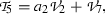
as

We observed that commutator Table 1 is skew-symmetric where (i, j)th entry of Table 1 is given by  . Even, the generators
  are linearly independent.
Then, taking any subgroup  to act on V, we have

where \(\Theta = \Theta (a_1,...,a_n,b_1,...,b_n)\) can be obtained by using the commutator table. The commutation relations are given in Table 1. Putting  and
and  in Eq. (15) with
For any \(b_j, 1 \le j \le 10\), it requires
Collecting the coefficients of all \(b_i\) in the above equation, ten differential equations about \(\phi (a_1,a_2,\dots ,a_{10})\) are obtained as
As per the following references [25, 26, 36], the general invariant function of the symmetry algebra \(L^{10}\) is
where F is an arbitrary function of two basic invariants \(a_1\) and \(a_5\) of Eq. (2). We form the adjoint matrix to get an optimal system of Eq. (2). The adjoint representation table of the ten-dimensional Lie algebra can be formulated in Table 2.
For \(F_i^s:g\rightarrow g\) defined by  is a linear map, for \(i=1,2,...,10\). The matrix \(M_i^\epsilon \) of \(F_i^\epsilon , i=1, 2, \dots , 10\) with respect to basis
  are given below:
Similarly, one can find other matrices; hence, using these ten matrices we obtain the adjoint group which is defined by the matrix

given in Appendix I.
3.1 Optimal system of one-dimensional Lie subalgebras
In order to form the one-dimensional optimal system of Eq. (2), For the vectors,  and
and  , we apply the adjoint transformations equation for Eq. (2) is given by
The following cases are considered to classify the one-dimensional Lie subalgebras of the resulted nonclassical symmetries.
Case 1 \(a_1 \ne 0, a_3=0, a_4 = 0, a_5 = 0, a_9 = 0\). Adopt one representative element  . Substituting \(\beta _1 =1, \beta _i=0, 2 \le i \le 10\) into Eq. (22), we get
\(\epsilon _6\) is an arbitrary constants.
Substituting \(a_1 = 0, a_5 = 0\) in Eq. (22) provides new invariants
Due to the Remark 2 in [36], we have following three instances as: \(a_3 a_9 (a_4)^{\frac{3}{2}} =1\), \(a_3 a_9 (a_4)^{\frac{3}{2}} =-1\) and \(a_3 a_9 (a_4)^{\frac{3}{2}}=0\). By virtue of second invariant, the following sub-cases are constructed and discussed below.
Case 2 \(a_3 \ne 0, a_i=0, i=1,2,4,\dots ,9\). Choose a representative element  . Substituting \(\beta _3=1, \, \beta _i=0, \, 1 \le i \le 10, \, i \ne 3\) into Eq. (22), we get
\(\epsilon _2,\epsilon _3,\epsilon _6,\epsilon _7,\epsilon _9\) and \(\epsilon _{10}\) are arbitrary constant.
Case 3 \(a_4 \ne 0, a_1=0, a_3=0, a_5 = 0, a_9 = 0\). Adopt one representative element  . Substituting \(\beta _4 =1, \beta _i=0, i = i=1,2,3,5,\dots ,10\) into Eq. (22), we get
\(\epsilon _2, \epsilon _6\) and \(\epsilon _8\) are arbitrary constants.
Case 4 \(a_6 \ne 0,\) \(a_i = 0, i=1,3,4,5,7,8,9,10\). Adopt one representative element  . Substituting \(\beta _6=1, \beta _i=0,i=1,\dots ,5,7,\dots ,10\) into Eq. (22), we get
\(\epsilon _i, i=2,3,4,6,7,8,10\) are arbitrary constants.
Case 5 \(a_2 \ne 0, a_7 \ne 0\). Adopt one representative element  . Substituting \(\beta _2=\beta _7=1, \beta _i=0,i=1,3,4,5,6,8,9,10\) into Eq. (22), we get
\(\epsilon _2, \epsilon _3, \epsilon _4,\epsilon _6,\epsilon _7\) and \(\epsilon _{10}\) are arbitrary constants.
Case 6 \(a_8 \ne 0, a_i=0, i=1,\dots ,7,9\). Adopt one representative element  . Substituting \(\beta _8 =1, \beta _i=0, i=1,\dots ,7,9,10\) into Eq. (22), we get
\(\epsilon _2, \epsilon _4, \epsilon _6,\epsilon _8,\epsilon _9\) and \(\epsilon _{10}\) are arbitrary constants.
Case 7 \(a_9 \ne 0, a_i=0, i=1,3,4,5,6,7\). Adopt one representative element  . Substituting \(\beta _9 =1, \beta _i=0, i=1,\dots ,8,10\) into Eq. (22), we get
\(\epsilon _2, \epsilon _4, \epsilon _6,\epsilon _8,\epsilon _9\) and \(\epsilon _{10}\) are arbitrary constants.
Case 8 \(a_6 \ne 0, a_7 \ne 0\). Adopt one representative element  . Substituting \(\beta _6 =\beta _7=1, \beta _i =0, i=1,\dots ,5,8,9,10\) into Eq. (22), we get
\(\epsilon _2, \epsilon _3, \epsilon _4,\epsilon _6,\epsilon _7\) and \(\epsilon _{10}\) are arbitrary constants.
Case 9 \(a_2 \ne 0, a_7 \ne 0,a_{10} \ne 0\). Adopt one representative element  . Substituting \(\beta _2=\beta _7=\beta _{10}=1, \beta _i =0, i=1,3,4,5,6,8,9\) into Eq. (22), we get
\(\epsilon _2, \epsilon _3, \epsilon _4,\epsilon _6,\epsilon _7\) and \(\epsilon _{10}\) are arbitrary constants.
Case 10 \(a_7 \ne 0,a_8 \ne 0, a_{10} \ne 0\). Adopt one representative element  . Substituting \(\beta _7 =\beta _8=\beta _{10}= 1, \beta _i =0, i=1,2,3,4,5,6,9\) into Eq. (22), we get
\(\epsilon _2, \epsilon _3, \epsilon _4,\epsilon _6,\epsilon _7\) and \(\epsilon _{10}\) are arbitrary constants.
Case 11 \(a_2 \ne 0, a_6 \ne 0\). Adopt one representative element  . Substituting \(\beta _2 =\beta _6=1, \beta _i =0, i=1,3,4,5,7,8,9,10\) into Eq. (22) we obtain the solution
\(\epsilon _2, \epsilon _3, \epsilon _4,\epsilon _6,\epsilon _7\) and \(\epsilon _{10}\) are arbitrary constants.
Similarly, we can find values of \(\epsilon _i\)’s for other members of optimal system. We concluded that the one-dimensional optimal system of subalgebra for KdV-type equation is as follows:
-
(1)

-
(2)

-
(3)

-
(4)

-
(5)
-
(6)

-
(7)

-
(8)
-
(9)

-
(10)

-
(11)


3.2 Optimal system of two-dimensional Lie subalgebras
Further, in this section we construct an optimal system of two-dimensional Lie subalgebras with the help of one-dimensional optimal system [4].
Let \(<W>\) be a one-dimensional Lie subalgebra from previous section and consider the problem of finding all two-dimensional Lie subalgebras containing \(<W>\). To construct such optimal system, we must find all possible \(V \in g\) such that \(<V, W>\) is a two-dimensional Lie subalgebra. As required, \(<V, W>\) to be a two-dimensional Lie subalgebra, there must be some constants \(\lambda \) and \(\mu \) such that
which are to be determined. Here, we must find V such that \(<V, W>\) is a two-dimensional vector space, and \(\lambda \) and \(\mu \) satisfy (24). This gives number of algebraic equations whose solutions will give the two-dimensional Lie subalgebras including \(<W>\).
To illustrate, we compute all two-dimensional Lie subalgebras which contain the one-dimensional Lie subalgebra \(<V_1>\). Let \(V = a_2 V_2 + \dots + a_9 V_9 + a_{10} V_{10}\) be a second basis element of a desired two-dimensional Lie subalgebra. Using Table 1, we obtain
which provides the left-hand side of Eq. (24). The problem here is to find \(a_2, \dots , a_{10}\) not simultaneously zero and \(\lambda \) and \(\mu \) such that
Case 1: When \(\mu = 0\) then, \(a_2=a_3= a_4= a_7= a_8= a_9=a_{10} = 0\). Any \(a_5\) and \(a_{6}\), not simultaneously zero, which is to be chosen arbitrarily. This gives a required member of two-dimensional Lie subalgebras \(<a_5 V_5 + a_{6} V_{6}, V_1>\), \((a_5, a_6)\) \(\in {\mathbb {R}}^2 \setminus {(0,0)}\).
Case 2: When \(\mu \ne 0\) then, \(a_5= a_6 = 0\). As \(V \ne 0, \mu =\frac{1}{4}\), is the only choice and \(a_2, a_3, a_4, a_7, a_8, a_9, a_{10}\) which is to be chosen arbitrarily. This gives a required member of two-dimensional Lie subalgebras \(<a_2 V_2+ a_3 V_3 +a_4 V_4 +a_7 V_7+ a_8 V_8 +a_9 V_9+ a_{10} V_{10}, V_1>, (a_2, a_3, a_4, a_7, a_8, a_9, a_{10}) \in {\mathbb {R}}^7 \setminus {(0,0,0,0,0,0,0)}\).
Secondly, we compute all two-dimensional Lie subalgebras which contain the one-dimensional Lie subalgebra \(<V_6>\). Let \(V = a_1 V_1 + \dots +a_5 V_5 +a_7 V_7+a_8 V_8+a_9 V_9 + a_{10} V_{10}\) be a second basis element of a desired two-dimensional Lie subalgebra. Using Table 1, we obtain
which provides the left-hand side of Eq. (24). The problem here is to find \(a_1, a_2, \dots , a_{10}\) not simultaneously zero and \(\lambda \) and \(\mu \) such that
Case 3: When \(\mu = 0\) then, \(a_9 =0\). Any \(a_1, a_3, a_4, a_5, a_7, a_8, a_9\) and \(a_{10}\) is not simultaneously zero, which is to be chosen arbitrarily. This gives a required member of two-dimensional Lie subalgebras \(<a_1 V_1 + \dots + a_5 V_5 +a_7 V_7+a_8 V_8 + a_{10} V_{10}, V_6>\), \((a_1, a_3, a_4, a_5, a_7, a_8, a_9, a_{10})\) \(\in {\mathbb {R}}^8 \setminus {(0,0,0,0,0,0,0,0)}\).
Case 4: When \(\mu \ne 0\) then, \(a_1= a_3= a_4= a_5= a_7= a_8= a_9=a_{10} = 0\). As \(V \ne 0, \mu =1\) is the only choice and \(a_2\), which is to be chosen arbitrarily. This gives a required member of two-dimensional Lie subalgebras \(<a_2 V_2, V_6>, a_2 \in {\mathbb {R}} \setminus {(0)}\).
This process, applied to all the one-dimensional Lie subalgebras from previous section, computes the two-dimensional Lie subalgebras which contain one-dimensional Lie subalgebras.
4 Group-invariant solutions
In this section, we restrict our study to the one-dimensional optimal system of Lie subalgebras computed in previous section. We derive several Lie symmetry reductions and corresponding group-invariant solutions with the help of one-dimensional optimal system of subalgebras.
4.1
Subalgebra
 :
:
 :
:For the infinitesimal generator

Thus, Eq. (13) becomes
which gives

where  is similarity function in which similarity variables X, Y and Z can be expressed as
Using Eq. (31) into Eq. (2), we get the following (2+1)-dimensional nonlinear reduced equation with variable coefficients as first reduction of the equation given as

where  , etc. To solve Eq. (33), we obtain new set of infinitesimal given as

where \(A_1\) and \(A_2\) are arbitrary constants.
4.1.1 For \(A_1 \ne 0, A_2 = 0\) in Eq. (34)
With the help of characteristic Eq. (13), then function F can be written as

through \(r = X Z^{\frac{1}{4}}\) and \(s= \frac{Y}{\sqrt{Z}}\). Putting the similarity form in Eq. (33), we have following reduced equation
We could not find generators of Eq. (36) because of high nonlinearity. Hence, this equation can be solved numerically.
4.1.2 For \(A_1 = 0, A_2 \ne 0\) in Eq. (34)
Using characteristic equations for this subcase, we obtain the similarity variables as follows

By substituting F in Eq. (33), we have
Again, we can find infinitesimals for Eq. (38) given as
where \(b_1\) is an arbitrary constant. Then, established characteristic equation for Eq. (39) is
We obtain the similarity variable as \(w = r \sqrt{s}\), and the similarity form is given by
Putting G in Eq. (38), we get
which is a highly nonlinear ODE. where \('\) denotes the derivative with respect to w. One particular result is given below
Using Eqs. (43), (41), (37) in Eq. (31), one obtains
4.2
Subalgebra
 :
:
 :
:Solving characteristic equations in this case yields

with \(X=x\), \(Y=y\), \(Z=z\). On inserting Eq. (45) into Eq. (2), reduced equation is

Then, the solution form for Eq. (46) is

with \(c_i \,(1 \le i \le 4)\) being arbitrary constants. Hence, Eq. (47) gives
Applying Lie symmetry method, Eq. (46) admits infinitesimals as

with \(\xi _X, \xi _Y , \xi _Z\) and  and \(A_i \,(1 \le i \le 7)\) being arbitrary constants. Moreover, some particular cases are discussed below.
4.2.1 Case \(A_2 \ne 0\)
Corresponding Lagrange’s equations are given below

By solving Eq. (50), we obtain

through \(r =X\) and \(s =Y\). Thus, we have

Substituting  where \(\zeta = a\,r +b \,s\) with a and b being constants in Eq. (52), we obtain an ordinary differential equation in H as
The general solution of (53) is given as
with \(c_1, c_2\) and \(c_3\) being arbitrary constants. Hence, using Eqs. (54) and (51), we obtain WeierstrassZeta function solution for governing KdV

The physical structures of Lump-type solitons and multi-solitons profiles for (55) with parameters \(c_1 = 154, c_2 = 0.003, c_3 = 2717\) for (a)–(f) and \(c_1 = 1, c_2 = 0.3, c_3 = 1\) for (g)–(i)
4.2.2 Case \(A_3 \ne 0\)
Lagrange’s system for this case is

By solving Eq. (56), we obtain

through similarity variables \(r =X/\sqrt{Y}\) and \(s =Z\). Substituting the value of  into Eq. (46), we obtain

Again, Eq. (58) admits infinitesimal generators as

where \(b_1\) and \(b_2\) are arbitrary constants. Using generators (59), solution G(r, s) takes the form as

where \(w= r \sqrt{s}\). Inserting Eq. (60) into Eq. (58), we have
Eq. (61) is a highly nonlinear ODE and cannot be solved easily. Assuming R(w) as polynomial with constants, we get
where \(\gamma \) is the arbitrary constant. Ultimately, group-invariant solution is
4.2.3 Case \(A_4 \ne 0\)
By solving characteristic equations, we obtain

with \(r =X\) and \(s =Z\). On inserting the value of  solution (64) into Eq. (46), we get

Similarity transformation method (STM) provides the following generators infinitesimal

where real parameters \(b_1, b_2\) and \(b_3\) are real arbitrary constants. Using Eq. (66), we obtain the solution  as
as

Inserting Eq. (67) into Eq. (65), we obtain ordinary differential equation as
Eq. (68) is a complex nonlinear ordinary differential equation. General solution is not easy to obtain, but one solution is given below
where real parameters \(\gamma \) are the arbitrary constant. Using Eqs. (69), (67), (64) in Eq. (45), corresponding rational function solution u is obtained as
4.2.4 Case \(A_5 \ne 0\)
The Lagrange’s equations read as

which produces

with variables \(r = Y\) and \(s = Z\). Thus, one obtains

The general solution is given as

Hence, using Eqs. (74), (72) in Eq. (45), the invariant solution is
with f being arbitrary function of y and z.
4.3
Subalgebra
 :
:
 :
:Using characteristic equation for  , we obtain

On inserting the similarity solution in Eq. (2), reduction equation is

Also, infinitesimals for Eq. (76) are

where \(A_i \,(1 \le i \le 5)\) are arbitrary constants. For completeness, reduced equations and invariant solutions for subcases are furnished in Table 3.

4.4
Subalgebra
 :
:
 :
:With the help of Lagrange system for  we found invariants as \(X=x, Y=y, T=t\) and
  . By putting u in Eq. (2), we get

The solution of Eq. (78) is

with \(c_1, c_2, c_3\) and \(c_4\) being arbitrary constants. Using Eq. (79), kink-type solution is obtained as
Moreover, by using wave transformation \(w = a X+ b Y- c T\) where a, b and c are constants in Eq. (78), putting \(F(x,y,t)=H(w)\), we get
Solving Eq. (81), we obtain
Eventually, solution of Eq. (2)
where \(a_1\) is an arbitrary constant.
4.5
Subalgebra
 :
:
 :
:4.5.1 For \(a_2=0\)
Subalgebra reduces to  , and using its characteristic equation the corresponding invariant form is

with \(X=x, Z=z, T=t\). On inserting solution in Eq. (2), we found the following reduction equation

The solution for Eq. (85) is

where \(c_1, c_2, c_3\) and \(c_4\) are arbitrary constants. Using Eq. (86) in Eq. (84), the kink-type solution of Eq. (2) is
Again, new set of infinitesimals for Eq. (85) are

where \(A_i \,(1 \le i \le 6)\) are arbitrary constants.
4.5.2 When \(A_1=0, A_3=0\) in Eq. (88)
Characteristic equations are given by

Using Eqs. (89), the solution with similarity variables is given by

Substituting the above invariant form in Eq. (85), the reduced equation is given as

Again, new set of infinitesimal generators are

where \(b_1, b_2\) and \(b_3\) are integral constants and group-invariant solution is

Using the value of  in Eq. (91), we have
Unfortunately, the solution for Eq. (94) is extremely difficult to solve analytically, and we can assume one particular solution given as
where b and c. Here, b in terms of other constants is given as follows
Hence, using Eqs. (95), (90) in (84), solution for Eq. (2) is given as
4.5.3 For \(a_2=1\)
Thus, corresponding subalgebra reduces to  , and using its characteristic equation, the similarity solution is

where the similarity variables \(X=x, Z=z, T=t\). Putting above value of u in (2), one obtain

The solution for Eq. (98) is given by

Hence, with the help of Eq. (99) in (97), one gets
The case for \(a_2=0\) is already discussed when we take subalgebra  . Similarly, we do for \(a_2=-1\) to obtain solution of Eq. (2).
4.6
Subalgebra
 :
:
 :
:Using the characteristic equation for  , we get

with \(Y=y, Z=z, T=t\). Making the use of u in (2), we have

By solving Eq. (102), we obtain

Hence, using Eq. (103) in Eq. (101), we get the desired group-invariant solution
Choosing two suitable values of arbitrary function \(g(\cdot ,\cdot )\) in the form of tanh function via Fig. 2 and sech function via Fig. 3 is demonstrated.

The physical structure of W-shaped soliton profile for (104) presents doubly soliton, traveling wave along the x-axis for \(g\left( \frac{t}{y},\frac{3zt-5y^2}{3t}\right) = \text {tanh}^2\left( \frac{3 t z-5 y^2}{3 y}\right) + \tanh ^2\left( \frac{2 t^3}{y^3}+\frac{2 \left( 3 t z-5 y^2\right) }{t}\right) +\text {tanh}^2\left( \frac{\left( 3 t z-5 y^2\right) ^2}{9 t^2}+\frac{2 t^2}{y^2}+1\right) \)

The physical struture of M-shaped soliton profile for (104) shows doubly soliton, and 2D plot exhibits solitary waves for \(g\left( \frac{t}{y},\frac{3zt-5y^2}{3t}\right) = \text {sech}^2\left( \frac{3 t z-5 y^2}{3 y}\right) + \text {sech}^2\left( \frac{2 t^3}{y^3}+\frac{2 \left( 3 t z-5 y^2\right) }{t}\right) +\text {sech}^2\left( \frac{\left( 3 t z-5 y^2\right) ^2}{9 t^2}+\frac{2 t^2}{y^2}+1\right) \)
4.7
Subalgebra
 :
:
 :
:For  , using characteristic equation we get

with invariants \(Y=y, Z=z, T=t\).

The physical structure of single soliton profile for (108) with \(g\left( \frac{z}{y},\frac{3zt-5y^2}{3z}\right) =\tanh \left[ \frac{3 t z-5 y^2}{3y}\right] ^2\) shows perspective view of the real part of the dark-bright soliton solution, the wave propagation pattern of the wave along the y-axis
Putting the above invariant solution in Eq. (2), we have

which has the general solution

Hence, using Eq. (107) in Eq. (105), we get the desired group-invariant solution is

The physical structure of single-soliton profile for (108) with \(g\left( \frac{z}{y},\frac{3zt-5y^2}{3z}\right) =\text {sech}\left[ \frac{3 t z-5 y^2}{3y}\right] ^2\) shows perspective view of the real part of the bright-dark soliton solution, the wave propagation pattern of the wave along the y-axis
Some particular solutions are shown in Figs. 4 and 5.
4.8
Subalgebra
 :
:
 :
:For \(a_6=1\),  becomes
  and using its characteristic equation, we get the desired invariant solution as
  , with \(X=x,Y=y-z\) and \(T=t\). Thus, the reduction equation is

By solving Eq. (109), we found the value of  as
as

with \(c_1, c_2\) and \(c_3\). Hence, using Eq. (110), the group-invariant solution in this case is
Following similar procedure we reduce Eq. (2) to ODEs and hence obtain solution for the case \(a_6=-1\).
4.9
Subalgebra
 :
:
 :
:In this case subalgebra is given by

and using corresponding characteristic equations, we have  , with \(X=x-y,Z=z\) and \(T=t\). Putting the value of u into (2), we have

Solving Eq. (112), we get

where \(c_1,\dots , c_4\) are arbitrary constants. Hence, one obtains
Moreover, generators of Eq. (112) are

where \(b_1, \dots , b_6\) are arbitrary constants. The characteristic equation is
Let \(b_3=b_1\), then group-invariant is

where
Reduced (1+1)-dimensional equation is given as
Under the condition \(b_6=\frac{b_4}{10}\), then above equation can be recast as
Using infinitesimals, we write characteristic equation as
Then, we obtained \( G(r,s)=\frac{d_2 r}{d_1}+R(w)\), where \(w=s\). We get the desired ODE as
The primitive is
Using back substitution, we obtain group-invariant solution is
4.10
Subalgebra
 :
:
 :
:For the infinitesimal generator

ultimately gives  , where \(Y=x-y(1+t),Z=z\) and \(T=t\). Putting the above value of u into governing equation, we have

Infinitesimals of Eq. (125) are

with \(\tilde{b_1}, \tilde{b_2}, \tilde{b_3}, \tilde{b_4}\) and \(\tilde{b_5}\) being the arbitrary constants.
Case I: If \(\tilde{b_1} \ne 0\), then using Eq. (126)

where \(b_1 = \frac{\tilde{b_4}}{\tilde{b_1}}, b_2=\frac{\tilde{b_3}}{\tilde{b_1}}, b_3=\frac{\tilde{b_2}}{\tilde{b_1}}, b_4=\frac{\tilde{b_5}}{\tilde{b_1}}\), then similarity forms of original equation yield

with similarity variable
The second reduction in this case
Clearly, one nontrivial solution of Eq. (130)
Eventually, group-invariant solution of Eq. (2)
which presents a parabolic wave profile in \(y-z\) plane.
Case II: If \(\tilde{b_1} = 0\), then using Eq. (126) then we obtain

then similarity forms of KdV-type equation yield

where similarity variables \(s=Z-\frac{b_3 T}{b_2}\) and \(r=X-\frac{b_4 Z}{b_3}\).
The second reduction of Eq. (2) produces
Infinitesimals of Eq (135) are
where \(d_1\) and \(d_2\) are arbitrary constants. In order to find corresponding third reduction using Eq. (136), we obtain the correspond group-invariant form
with \(w=s\), which leads to ordinary differential equation given as
The solution of (138) is
Eventually, the group-invariant solution of (2) is
which exhibits also a parabolic wave profile in x, y, z, t.
Remark
The obtained group-invariant solutions including the WeierstrassZeta function, M-shaped solitons, W-shaped solitons, multi-solitons and rational function solutions which are entirely different compared to other researchers works [29, 32,33,34]. Also, the different dynamical structures of these solutions have rich localized structures due to the existence of free parameters in the infinitesimals.
4.11
Subalgebra
 :
:
 :
:For the infinitesimal generator

we have following characteristic equation
The similarity form of the solution of Eq. (2)

with similarity variables \(X=x, Y=y\) and \(T=t\). Inserting the value of u into (2), we have

To solve Eq. (143), we obtain new set of infinitesimal generators given as

where \(A_1,A_2,A_3,A_4,A_5,A_6,A_7\) and \(A_8\) are arbitrary constants.
For \(A_2, A_5, A_7\) and \(A_8\) being nonzero and taking all other constants zero, we obtain following characteristic equations

The function  can be written as

through \(r=X-T, s = Y-T\). Putting the similarity form in Eq. (143), we have following reduced equation
Again we can find infinitesimals for Eq. (143) given as
where \(B_1,B_2,B_3,B_4\) are arbitrary constants. Let us take \(B_1 = 0 \), then the desired characteristic equations are given as
We obtain the similarity variable as \(w= r-\frac{B_3}{B_2}\), and the similarity form is given by
Putting G in Eq. (147), we obtain
Primitives for Eq. (151) are
where \(\xi = -239B_2^2+22B_2B_3+B_3^2+228B_2B_4-12B_3B_4+36 B_4^2\) and \(\alpha \) is an arbitrary constant. Using Eqs (152), (150), (146) in (142), we obtain
In summary, the physical interpretation of the resulting soliton solutions is illustrated by various three-dimensional, two-dimensional and contour graphs through numerical simulation. The constructed group-invariant solutions involve many arbitrary constants and arbitrary functions, thereby exhibiting rich physical structures and including the existing solutions in the literature.
5 Adjoint equation and conservation laws
5.1 Necessary preliminaries and adjoint equation
For a given differential equation, there is a close connection between Lie symmetries and conservation laws as established by Noether’s theorem. To derive conservation laws of Eq. (2), we use the following Theorem proved by Ibragimov [6, 38].
Theorem 1
Any symmetry (Lie point, Lie-Bäcklund, nonlocal symmetry)
of Eq. (2) provides a conservation law \({\mathcal {D}}_i(C_i) = 0\) for the system consisting of Eq. (2) and the adjoint equation

The conserved vector is given by
where W and \({\mathcal {L}}\) are defined as
For a conserved vector, the following conservation equation holds:
where \({\mathcal {C}}^x = {\mathcal {C}}^x(t,x,y,z,u,...)\), \({\mathcal {C}}^y = {\mathcal {C}}^y(t,x,y,z,u,...)\), \({\mathcal {C}}^z = {\mathcal {C}}^z(t,x,y,z,u,...)\), \({\mathcal {C}}^t = {\mathcal {C}}^t(t,x,y,z,u,...)\).
A formal Lagrangian for three-dimensional KdV-type equation is
Here, p(x, y, z, t) is a new dependent variable also known as adjoint variable. According to Eq. (161), we obtain
The adjoint equation for (3+1)-dimensional KdV-type equation is given by
where
where \({\mathcal {D}}_x , {\mathcal {D}}_y, {\mathcal {D}}_z\) and \({\mathcal {D}}_t\) denote the total differentiation with respect to x, y, z and t, respectively. Substituting Eq. (164) into Eq. (163), the adjoint equation for the (3+1)-dimensional KdV-type equation is expressed by
Clearly, when \(p=u\), we obtain
It is easily obtain that on substituting u instead of p in adjoint equation (2) is not recovered. Thus, (3+1)-dimensional KdV-type equation is not self-adjoint ”.
5.2 Conservation laws
Using Lagrangian in Eq. (161) and Theorem 1 for Eq. (2), the general form of conservation laws is given as
with \(W = \eta -\xi _x u_x - \xi _y u_y- \tau u_t\).
In this article, we consider conservation laws related with two infinitesimal symmetries  and
and  . They are given as follows: For the symmetry
  , we have \(W = -u_t\). Now, using Eqs. (162) in Eq. (167), the corresponding conservation laws are
For the symmetry  , we have \(W = -u_x\). Now, using Eqs. (162) in Eq. (167), the corresponding conservation laws are
Similarly, one can obtain other conservation laws corresponding to each Lie point symmetry. Making use of explicit solutions of Eq. (165), nonlocal conservation laws in case of each Lie point symmetries can be obtained for (3+1)-dimensional KdV-type equation.
6 Results and discussion
The exact analytical wave solutions are obtained with the help of symbolic computation via Lie symmetry analysis for a (3+1)-KdV equation. The dynamical behavior of obtained solutions demonstrates the different lump-type soliton solutions for adequate choice of arbitrary independent functions and free parameters. Some important physical structures are obtained, and a summary of the profiles of the solutions is as follows:
Figure 1 shows the physical structures of Lump-type solitons and multi-soliton profiles for (55) with parameters \(c_1 = 154, c_2 = 0.003, c_3 = 2717\). Properties of such solitons reveal that solitons do not transform their size and shapes when they are associated with each other and complete elastic nature is described by the wave structures. In this figure, we have shown elastic behavior with parameters (a) \(a=0.3, b=1\), (b) \(a=1, b=1\), (c) \(a=1.5, b=1\), (d) \(a=0.3, b=4\), (e) \(a=1, b=4\), (f) \(a=1.5, b=4\). Moreover, annihilation has been achieved for parameters (g) \(a=1, b=1, c_1=1, c_2=0.3, c_3=1\), (h) \(a=1, b=5, c_1=1, c_2=0.3, c_3=1\), (i) \(a=1, b=20, c_1=1, c_2=0.3, c_3=1\). In this figure, we have observed annihilation of multisoliton into a stationery wave profile for Eq. (55) by changing the specific arbitrary constants as \( c_1=1, c_2=0.3, c_3=1\).
Figure 2 exhibits the physical structure of W-shaped soliton profile for (104) presents doubly soliton, traveling wave along the x-axis for \(g\left( \frac{t}{y},\frac{3zt-5y^2}{3t}\right) = \text {tanh}^2\left( \frac{3 t z-5 y^2}{3 y}\right) + \tanh ^2\left( \frac{2 t^3}{y^3}+\frac{2 \left( 3 t z-5 y^2\right) }{t}\right) +\text {tanh}^2\left( \frac{\left( 3 t z-5 y^2\right) ^2}{9 t^2}+\frac{2 t^2}{y^2}+1\right) \). Moreover, two-dimensional wave profiles and contour plots are demonstrated in this figure for parameters \(z=0.9654, t=6\) and \(x=1,5,10\). An important observation is the amplitude, the velocity and the shape of the soliton remains constant.
Figure 3 shows the physical struture of M-shaped soliton profile for (104) shows doubly soliton; 2D plot exhibits solitary waves for \(g\left( \frac{t}{y},\frac{3zt-5y^2}{3t}\right) = \text {sech}^2\left( \frac{3 t z-5 y^2}{3 y}\right) + \text {sech}^2\left( \frac{2 t^3}{y^3}+\frac{2 \left( 3 t z-5 y^2\right) }{t}\right) +\text {sech}^2\left( \frac{\left( 3 t z-5 y^2\right) ^2}{9 t^2}+\frac{2 t^2}{y^2}+1\right) \). In this figure, three-dimensional plot is sketched using \(z=0.9654, t=6\), two-dimensional plot shows M-wave propagation for \(x=3.5, z=0.9654\) and a contour plot is also exhibited for \(z=0.9654, t=6\). Such solitary waves type precisely M-shaped and W-shaped solitons described the propagation of ultrashort pulses in optical fibers [39].
Figure 4 represents V-type physical structure of single soliton profile for (108) with \(g\left( \frac{z}{y},\frac{3zt-5y^2}{3z}\right) =\tanh \left[ \frac{3 t z-5 y^2}{3y}\right] ^2\) shows perspective view of the real part of the dark-bright soliton solution and the wave propagation pattern of the wave along the y-axis. It includes three-dimensional plots for \(z=1, t=15\), wave propagation using two-dimensional plot for \(x=2, z=1, t=15\) and contour plot for \(z=1, t=15\).
Figure 5 exhibits the physical structure of single soliton profile for (108) with \(g\left( \frac{z}{y},\frac{3zt-5y^2}{3z}\right) =\text {sech}\left[ \frac{3 t z-5 y^2}{3y}\right] ^2\) and shows perspective view of the real part of the bright-dark soliton solution, the wave propagation pattern of the wave along the y-axis. It includes three-dimensional plot for \(z=1, t=14\), wave propagation using two-dimensional plot for \(x=2, z=1, t=14\) and contour plot for \(z=1, t=14\). Such types of solutions are new soliton solutions obtained in this work that can help us with understanding the propagation of solitons through a nonlinear medium.
Figure 6 shows the physical structure of Kink wave soliton profile (111) for \(c_1 = 0.4873\), \(c_2 = 0.3374\) and \(c_3 = 0.3984\) which describes strip single soliton in 3D plot; 2D plot with three values of x and corresponding contour shape [40]. Using the values of certain free parameters, we can control the solitons propagation direction and speed and reduce the interactions between them as well.

The physical structure of kink wave soliton profile (111) for \(c_1 = 0.4873\), \(c_2 = 0.3374\) and \(c_3 = 0.3984\) shows strip single soliton in 3D plot; 2D plot with three values of x and corresponding contour shape
It is interesting to notify that the established solutions in this article have not been reported in the literature. Furthermore, the wide diversity of features and physical parameters of these generated soliton solutions are illustrated with the assistance of 3D plots, considering the suitable choice of involved arbitrary independent functions and other constants. Such type of investigation is highly recommended in the areas of progressive research and development.
7 Conclusion
Applications of the Lie group-theoretic method are well defined for constructing Lie point symmetries and group-invariant solutions of three-dimensional KdV-type equation. The geometric vector fields spanned by ten basic Lie point symmetries are obtained with the help of computerized symbolic computation Maple. An optimal system of ten symmetry subalgebras is established to classify all the symmetry reductions. By using the optimal system, Eq. (2) is converted into numerous NPDEs with less order. In this work, symbolic computation is used for numerical simulation of various solutions and different types of solutions are derived and interpreted via three-dimensional and two-dimensional graphs through Mathematica 11.3. The obtained solutions are given by equations (44), (55), (70), (75), (80), (83), (96), (104), (108), (111), (100), (114), (124), (132), (140) which are entirely different compared to the works [33, 34]. Using the Ibragimov approach, we constructed nonlocal conservation laws for some Lie point symmetries. The obtained conservation laws can be used in the construction of new numerical schemes and stability analysis of solutions so obtained. Some exact analytic solutions in the shapes of kink waves, traveling waves, single solitons, doubly solitons, curved-shaped multi-solitons and explicit WeierstrassZeta are constructed by Lie group of transformation method. Moreover, this work reveals that some traveling waves which propagate are solitary wave types precisely M-shaped, W-shaped solitons and dark-bright solitons.
References
G.B. Whitham, Linear and Nonlinear Waves (Wiley, New York, 1974)
P.J. Olver, Applications of Lie Groups to Differential Equations (Springer, Berlin, 1991)
G.W. Bluman, S. Kumei, Symmetries and Differential Equations (Springer, Berlin, 1989)
L.V. Ovsiannikov, Group Analysis of Differential Equations (Academic, New York, 1982)
P.J. Olver, P. Rosenau, Group-invariant solutions of differential equations. SIAM J. Appl. Math. 47, 263–278 (1987)
N.H. Ibragimov, A new conservation theorem. J. Math. Anal. Appl. 333, 311–328 (2007)
S.V. Meleshko, Group classification of the equations of two dimensional motions of a gas. J. Appl. Maths. Mech. 58, 629–635 (1994)
N.H. Ibragimov, M. Torrisi, A. Valenti, Preliminary group classification of equations \( v_{tt} = f(x, v_x ) v_{xx} + g(x, v_x ) \). J. Math. Phys. 32, 2988 (1991)
Y. Zhang, W.X. Ma, Rational solutions to a KdV-like equation. Appl. Math. Comp. 256, 252–256 (2015)
F. Batool, G. Akram, New solitary wave solutions of the time-fractional Cahn-Allen equation via the improved \(\left(\frac{G^{\prime }}{G}\right)\)-expansion method. Eur. Phys. J. Plus 133, 171 (2018)
D.J. Korteweg, G. Vries, On the change of form of long waves advancing in a rectangular canal, and on a new type of long stationary wave. Philos. Mag. 39, 422–443 (1895)
A.J. Khattak, A comparative study of numerical solutions of a class of KdV equation. App. Math. Comput. 199, 425–434 (2008)
S.A. Khuri, Soliton and periodic solutions for higher order wave equations of KdV type. Chaos Solitons Fractals 26, 25–32 (2005)
N.J. Zabusky, M.D. Kruskal, Interaction of solitons in a collisionless plasma and the recurrence of initial states. Phys. Rev. Lett. 15, 240–243 (1965)
J.M. Miles, Solitary waves. Ann. Rev. Fluid Mech. 12, 11–43 (1980)
O. Darrigol, Worlds of Flow (Oxford University Press, Oxford, 2005)
R. Hirota, The Direct Method in Soliton Theory, 155 (Cambridge University Press, Cambridge, 2004)
M. Wang, Y. Zhou, Z. Li, Application of a homogeneous balance method to exact solutions of nonlinear equations in mathematical physics. Phys. Lett. A 216, 67–75 (1996)
A. Biswas, D. Milovic, Bright and dark solitons of the generalized nonlinear Schrödinger’s equation. Commun. Nonlinear Sci. Numer. Simul. 15, 1473–1484 (2010)
N.A. Kudryashov, Simplest equation method to look for exact solutions of nonlinear differential equations. Chaos Solitons Fractals 24, 1217–1231 (2005)
M. Lakshmanan, P. Kaliappan, Lie transformations, nonlinear evolution equations, and Painlevé forms. J. Math. Phys. 24, 795–806 (1983)
M. Kumar, R. Kumar, A. Kumar, On similarity solutions of Zabolotskaya-Khokhlov equation Comput. Math. Appl. 68, 454–463 (2018)
M. Xu, M. Jia, Exact solutions, symmetry reductions, painlevé test and Bäcklund transformations of a coupled KdV equation. Commun. Theor. Phys. 68, 417–444 (2017)
S. Kumar, D. Kumar, Solitary wave solutions of (3+1)-dimensional extended Zakharov-Kuznetsov equation by Lie symmetry approach Comput. Math. Appl. 77(8), 2096–2113 (2019)
S. Kumar, D. Kumar, A.M. Wazwaz, Group invariant solutions of (3+1)-dimensional generalized B-type Kadomstsev Petviashvili equation using optimal system of Lie subalgebra. Phys. Scr. 94 (2019)
D. Kumar, S. Kumar, Some new periodic solitary wave solutions of (3+1)-dimensional generalized shallow water wave equation by Lie symmetry approach. Comput. Math. Appl. 78, 857–877 (2019)
S. Kumar, A. Kumar, H. Kharbanda, Lie symmetry analysis and generalized invariant solutions of (2+1)-dimensional dispersive long wave (DLW) equations. Phys. Scr. 95 (2020)
D.V. Tanwar, A.M. Wazwaz, Lie symmetries and dynamics of exact solutions of dissipative Zabolotskaya-Khokhlov equation in nonlinear acoustics. Eur. Phys. J. Plus 135, 520 (2020)
S.Y. Lou, Dromion like structures in a (3 + 1) dimensional KdV-type equation. J. Phys. A Math. Gen. 29, 5989–6001 (1996)
A.M. Wazwaz, Soliton solutions for two (3+1)-dimensional non-integrable KdV-type equations. Math. Comp. Mod. 55, 1845–1848 (2012)
W. Hereman, A. Nuseir, Symbolic methods to construct exact solutions of nonlinear partial differential equations. Math. Comput. Simul. 43, 13–27 (1997)
Ö. Ünsal, Complexiton solutions for (3+1)-dimensional KdV-type equation. Comp. Math. Appl. 75(7), 2466–2472 (2018)
N. Liu, Y. Liu, Homoclinic breather wave, rouge wave and interaction solutions for a (3+1)-dimensional KdV-type equation. Phys. Scr. 94 (2018)
J.J. Mao, S.F. Tian, T.T. Zhang, Rogue waves, homoclinic breather waves and soliton waves for a (3+1)-dimensional nonintegrable KdV-type equation. Int. J. Numer. Method H 29, 763–772 (2019)
A.M. Wazwaz, New solutions for two integrable cases of a generalized fifth-order nonlinear equation. Mod. Phys. Lett. B 29, 1550065 (2015)
X. Hu, Y. Li, Y. Chen, A direct algorithm of one dimensional optimal system for the group invariant solutions. J. Math. Phys. 56 (2015)
P. Satapathy, T.R. Sekhar, Optimal system, invariant solutions and evolution of weak discontinuity for isentropic drift flux model. Appl. Math. Comp. 334, 107–116 (2018)
N.H. Ibragimov, Nonlinear self-adjointness and conservation laws. J. Phys. A Math. Theor. 44 (2011)
G. Dieu-donne, C.G.L. Tiofack, A. Seadawy et al., Propagation of W-shaped, M-shaped and other exotic optical solitons in the perturbed Fokas-Lenells equation. Eur. Phys. J. Plus 135, 371 (2020)
S. Kumar, D. Kumar, A. Kumar, Lie symmetry analysis for obtaining the abundant exact solutions, optimal system and dynamics of solitons for a higher-dimensional Fokas equation. Chaos Soliton Fractals 142 (2021)
Author information
Authors and Affiliations
Corresponding author
Ethics declarations
Conflict of interest
None.
Appendix I
Appendix I
where \(A_{ij}\) are given below
Rights and permissions
About this article

Cite this article
Kumar, S., Kumar, D. & Wazwaz, AM. Lie symmetries, optimal system, group-invariant solutions and dynamical behaviors of solitary wave solutions for a (3+1)-dimensional KdV-type equation. Eur. Phys. J. Plus 136, 531 (2021). https://doi.org/10.1140/epjp/s13360-021-01528-3
Received:
Accepted:
Published:
DOI: https://doi.org/10.1140/epjp/s13360-021-01528-3