
Abstract
In the present study, we report here the flow curve prediction of AlCoCrFeNi2.1 eutectic high entropy alloy (EHEA) at different temperatures and strain rates using different modeling techniques such as physics-based [modified Zerilli–Armstrong (ZA) model], phenomenological [modified Johnson–Cook (JC) model, Arrhenius model], and artificial neural network (ANN) modeling. Finally, the performance of all conventional (i.e., physics-based and phenomenological) and ANN modeling was evaluated by coefficient correlation (R) and average absolute relative error (AARE) parameters. It is found that the flow curve prediction by phenomenological modeling [i.e., modified JC model (R = 0.9646, AARE = 19.41%) and Arrhenius model (R = 0.9696, AARE = 14.62%)] is better as compared to physics-based modified ZA model (R = 0.9321, AARE = 21.42%). A comparative evaluation of obtained simulated results indicates that the prediction of hot deformation behavior of studied EHEA using ANN modeling (where R = 0.9985, and AARE = 4.57%) is matching excellently with experimental flow curve results as compared to conventional modeling approaches.
Introduction
Multicomponent high entropy alloys (HEAs) have been attracting attention worldwide and constitute an active, frontier area of research in the exploration of novel materials development with unseen properties since the pioneering work of Cantor et al. (2004) and Yeh et al. (2004) on these alloys in 2004. The search for novel HEA with unique microstructure is being actively pursued as a major step towards realizing the potential applications. It is reported that eutectic HEAs (EHEAs) having high thermal stability and unique properties open up new opportunities for creating next-generation engineering materials. Therefore, understanding the flow curve behavior during hot deformation is extremely important for the manufacturing of materials. Since the hot deformation processing of materials is a complex phenomenon. During the deformation, the hardening and softening mechanism depends on the thermomechanical processing parameters such as temperature, strain, and strain rate (Jain et al. 2020b; Samal et al. 2016; Rahul et al. 2018). Microstructural development and mechanical properties of materials are interconnected during hot deformation and can be understood by a different flow mechanism (Huang and Logé 2016). Microstructural changes during the processing affect mechanical properties such as flow stress. Understanding the flow behavior of HEAs during hot working conditions helps in designing the alloy for high-temperature applications. The different mechanisms associated with the hot deformation of materials are work hardening, softening, and dynamic recrystallization (Huang and Logé 2016; Alaneme and Okotete 2019). The different constitutive models are also used to understand thermomechanical processing of materials and are categorized as phenomenological, physics-based, and artificial neural network (ANN) models (Lin and Chen 2011; Murugesan and Jung 2019). It is to be noted that a phenomenological model based on mathematical functions provides information regarding flow stress but not about the physical significance of the process. The calibration of that model is easy due to the limited material constant to predict the flow stress, but that model is not applicable to a wide range of strain rate and temperature (Murugesan and Jung 2019). In phenomenological models, flow stress is the function of temperatures, stress, and strain rates. Those models are based on the classical approach for determining the prediction of flow stress for materials. Further, in the phenomenological model, the prediction of material properties is based on fitting and regression of experimental results at higher strain rate and temperature during the thermomechanical processing of materials. However, it is found that this model fails to predict the material behavior accurately. Further, the physics-based model provides information regarding the thermodynamics, dislocation, and kinetics of materials. Materials constant calculation for the above-discussed model is based on regression fitting. Also, due to the non-linear flow stress behavior with temperature and strain rate during hot deformation of materials, the regression analysis for flow stress prediction is not accurate (Lin and Chen 2011).
Recently, artificial neural network (ANN) models have attracted researchers to design materials for different applications and predict mechanical properties for high-temperature applications (Altinkok and Koker 2004; Hattab and Motelica-Heino 2014; Jain et al. 2020a). ANN model can solve a complex problem with good accuracy as compared to a conventional model. ANN approach is based on the human brain, the neural network mainly consists of different layers, and each layer has neurons that collect and transfer the data to the layer (Sabokpa et al. 2012). First input parameter as a signal is collected by each neuron in the input layer and then these signals transfer to the hidden layer and, subsequently, the layer activation function transfers the signals to the output layer. Patnamsetty et al. (2020) reported the flow stress prediction using a constitutive model for CoCrFeMnNi HEA and found that the predicted output is an accurate track with experimental results in a broad range of temperature and strain rates. Motlagh et al. (2020) reported the hot deformation prediction of 1.4542 Stainless Steel using different constitutive models and found that the suggested model prediction is accurate and tracked with experimental results. Sani et al. (2018) reported the prediction of the flow behavior of Mg alloy (at a temperature range 250–450 °C and strain rates range 0.001–1 s−1) by constitutive and ANN modeling approaches and obtained results show that the ANN model prediction is better than the constitutive model. Jain et al. (2020b) recently reported that the prediction of the flow curve using ANN modeling is well matched with the experimental flow curve compared to the results obtained using the constitutive model for novel Co–Cr–Fe–Ni–Zr quasi-peritectic HEA.
Considerable literature is available on various aspects of HEAs, including the development of novel HEAs and microstructure-property correlation. It is worth mentioning that the subject of the mechanical behavior of materials, followed by correlation with microstructure, has also been adequately covered in the literature (Miracle and Senkov 2017; Chen et al. 2018). The different modeling techniques, including physics-based modeling, phenomenological modeling, and artificial neural network (ANN), prove to be useful tools in the analysis of materials flow behavior. In the current study, the conventional and ANN models are used to predict the hot deformation flow curve of the studied EHEA. The conventional models have specific limitations to predict the flow behavior, such as JC model has not considered the thermal softening effect for flow stress prediction, while physics-based ZA model considers the strain hardening, thermal softening, and other physical effects for flow stress prediction, but uses some parameters which are estimated using precision equipment. The main objective is to develop different modeling approaches that predict the hot deformation behavior of the studied EHEA at different hot working conditions with great accuracy.
Modeling Details
The experimental flow stress data were collected from a previous study conducted by Rahul MR and their coworkers on EHEA under various hot deformation conditions, including temperature ranges of 900–1100 °C and strain rate ranges of 0.001–10 s−1 (Rahul et al. 2018). In this study, three different types of models such as the physics-based, phenomenological, and ANN models, are used to predict the flow behavior of EHEA. It is to be noted here that the modified Zerilli–Armstrong (ZA) model, modified Johnson–Cook (JC) model, Arrhenius-type constitutive equations, and ANN model with backpropagation training algorithm are used for predicting the flow stress. The different model's accuracy or performance is evaluated by the following parameters: coefficient of correlation (R) and average absolute relative error (AARE).
Results and Discussion
Modified Zerilli–Armstrong (ZA) Model
The simple ZA model is based on dislocation mechanisms which primarily is the cause of inelastic behavior under several load conditions (Lin and Chen 2011). The effects of strain hardening, strain rate hardening, and thermal softening on flow stress are considered. However, the simple ZA model considers only the coupling effect of temperature and strain rate. While the modified ZA model assumes the coupling effects of both temperature and strain rate as well as temperature and strain. The modified ZA model is represented by the following equation (Lin and Chen 2011; Murugesan and Jung 2019; Niu et al. 2020):
where C1, C2, C3, C4, C5, C6, and n are material constants and T* = T–Tr, Tr being the reference temperature, is taken as 900 °C and \(\dot{\varepsilon }^{*}\) (ratio of strain rate to reference strain rate) which is taken as 1 s−1. The following procedure has been employed to determine all the material constants:
-
(i)
First, C1 is to be determined from flow curves at reference conditions. Actually, C1 is the reference yield stress (at reference strain rate and temperature conditions), i.e., at 900 °C and 1 s−1. C1 was found to be 298.77 MPa.
-
(ii)
C2 and n are to be determined at reference strain rate using the following equation:
$$\sigma = \left( {C_{1} + C_{2} \varepsilon^{n} } \right) \exp \left[ { - \left( {C_{3} + C_{4} \varepsilon } \right)T^{*} } \right].$$(2)
Taking natural logarithm and introducing two parameters I1 and S1 such that
We get
By putting the flow stress–strain data at reference strain rate 1 s−1, the values of S1 and I1 can be determined from the slope and intercept of ln \(\sigma\) vs. T* at every discrete strain, as shown in Fig. 1a. Now, to find C2 and n, the following equation is used:
lnC2 and n are the intercept and slope of \(\ln \left( {\exp \left( {I_{1} } \right) - C_{1} } \right)\) vs. \(\ln \varepsilon\) linear fit curve (given in Fig. 1b). C2 and n are found to be 63.213005 and − 0.14001898, respectively.

Calculation of material constant for modified ZA model
-
(iii)
Now to find C3 and C4, the expression of S1 is used:
$$S_{1 } = - \left( {C_{3} + C_{4} \varepsilon } \right).$$(7)For every strain, S1 is obtained. In the S1 vs. \(\varepsilon\) linear fit curve (given in Fig. 1c), the slope is −C3, and the intercept is −C4. Thus, C3 and C4 are found to be 0.00379014 and 0.00117786, respectively.
-
(iv)
C5 and C6 can be found by taking the natural logarithm of Eq. (1) and introducing a new parameter S2 such that:
$$\ln \sigma = \ln \left( {C_{1} + C_{2} \varepsilon^{n} } \right) - \left( {C_{3} + C_{4} \varepsilon } \right)T^{*} + S_{2} \ln \dot{\varepsilon }^{*}$$(8)$$S_{2 } = C_{5} + C_{6} T^{*} .$$(9)
For all the temperatures and discrete strains, S2 is to be found by the slope of the \(\ln \sigma\) vs. \(\ln \dot{\varepsilon }^{*}\) linear fit curve. Then, C5 and C6 are found from the slope and intercept of S2 vs. T* linear fit at every discrete strain (given in Fig. 1d). The final C5 and C6 are the average of all C5 and C6 at each strain. Thus, C5 and C6 are found to be 0.164199 and 0.00039463, respectively. Now finally, the obtained modified ZA equation is expressed:
The predicted and experimental flow curve at different thermomechanical conditions employing a modified ZA model is given in Fig. 2.

Predicted and experimental flow stress at different hot working conditions using a modified ZA model
Modified Johnson–Cook Model for Flow Stress Prediction
In the J–C model, flow stress is dependent on the temperature, strain, and strain rate which is used for different types of materials and a more comprehensive range of temperature and strain rate due to the simplicity and easy availability of model parameters. In a simple JC model, the relationship between the deformation temperature, flow stress, strain rate, and strain can be expressed as (Murugesan and Jung 2019; Motlagh et al. 2020; Niu et al. 2020; Samantaray et al. 2009; He et al. 2018):
where the \(\sigma\) is flow stress, \(\sigma_{y}\) is the reference yield stress (at the reference temperature and strain), A is strain hardening coefficient, n is strain hardening exponent, B is coefficient of strain rate hardening, m is the thermal softening coefficient, \(\dot{\varepsilon }^{*}\) dimensionless coefficient (ratio of strain rate \(\dot{\varepsilon }\) and \(\dot{\varepsilon }_{{\text{r}}}\) reference strain rate), and T* is homologous temperature. T* can be expressed as:
where the T is the hot working temperature, \(T_{{\text{m}}}\) is the melting temperature, and \(T_{{\text{r}}}\) is the reference temperature. The minimum value of temperature and strain rate during hot working is assumed to be the reference value. However, it is observed that the temperature and strain rate do not have independent effects on flow stress. This leads to a new modified Johnson cook model, which identifies the coupling effects of temperature and strain rates (Zhang et al. 2017). The modified Johnson Cook (JC) model can be expressed as:
where A1, B1, B2, C1, \(\lambda_{1}\), and \(\lambda_{2}\) are materials constants. The meanings of the rest of the variables are the same as those in the simple JC model.
The following procedure is employed to determine these material constants:
-
(a)
First, to determine A1, B1, and B2, a two-degree polynomial fitting is done at a reference temperature of 1100 °C (not taken minimum in modified JC model) and reference strain rate of 1 s−1 (given in Fig. 3a). The stress would now be evaluated in the reference conditions by the following expression:
$$\sigma = \left( {A_{1} + B_{1} \varepsilon + B_{2} \varepsilon^{2} } \right).$$(14)Fig. 3 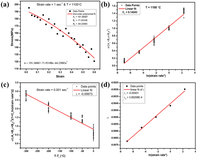
Calculation of material constant for modified JC model
On performing a two-degree linear fit for all chosen discrete strains (0.025–0.6) at reference conditions, we get A1, B1, B2 as 191.5067, − 71.93108, − 64.23083, respectively, from the coefficient of fitted polynomial equation.
-
(b)
Now for determining C1, only reference temperature (1100 °C) is used. In this condition, we get the following equation:
$$\frac{\sigma }{{\left( {A_{1} + B_{1} \varepsilon + B_{2} \varepsilon^{2} } \right)}} = 1 + C_{1} \ln \dot{\varepsilon }^{*} .$$(15)Thus, from the given expression, C1 is the slope of \(\frac{\sigma }{{\left( {A_{1} + B_{1} \varepsilon + B_{2} \varepsilon^{2} } \right)}}\) vs. \(\ln \dot{\varepsilon }^{*}\) (given in Fig. 3b). This needs to be done for all discrete strains and strain rates in a single graph. C1 is determined as 0.1424.
-
(c)
Next to determine \(\lambda_{1}\), \(\lambda_{2}\), the following expression is used, which is results from rearranging the modified JC equation and taking its logarithm, we get
$$\ln \frac{\sigma }{{\left( {A_{1} + B_{1} \varepsilon + B_{2} \varepsilon^{2} } \right)\left( {1 + C_{1} \ln \dot{\varepsilon }^{*} } \right)}} = \left( {\lambda_{1} + \lambda_{2} \ln \dot{\varepsilon }^{*} } \right)\left( {T - T_{{\text{r}}} } \right).$$(16)

To simplify this equation, a parameter λ is introduced such that:
λ can be easily determined as it is the slope of the \(\ln \frac{\sigma }{{\left( {A_{1} + B_{1} \varepsilon + B_{2} \varepsilon^{2} } \right)\left( {1 + C_{1} \ln \dot{\varepsilon }^{*} } \right)}}\) vs. \(\left( {T - T_{{\text{r}}} } \right)\) given in Fig. 3c. Similarly, a different λ for every strain rate is obtained. Hence, \(\lambda_{1}\), \(\lambda_{2}\), can be easily found from the intercept and slope of λ vs. \(\ln \dot{\varepsilon }^{*}\) plot, which is presented in Fig. 3d. \(\lambda_{1}\) and \(\lambda_{2}\) are found to be − 0.00401 and 0.000395208, respectively. Thus, the final modified JC equation can be expressed as follows:
The predicted and experimental flow stress at different hot working conditions using a modified JC model is given in Fig. 4.

Predicted and experimental flow stress at different hot working conditions using a modified JC model
Arrhenius Model
In this model, hot deformation flow behavior during hot working of materials can be predicted by using the constitutive equation. In the equation, flow stress is the function of different hot working variables such as temperature, strain, and strain rate. The equation can be written as follows considering the Zener–Holloman parameter (Z) (Saravanan and Senthilvelan 2016; Gao et al. 2018):
In the above equation, \(\dot{\varepsilon }\) is strain rate (s−1), Q is the activation energy (J mol−1), R is the universal gas constant 8.314 J−1mol−1 K−1, T is deformation temperature in K, σ is hot deformation stress (MPa), and A, α (α = β/N), and n are materials constant. The value of different material constants is calculated by linear fitting of different plots mentioned in Fig. 5. The values β and N are the slopes of the lnσ vs. ln\(\dot{\varepsilon }\) and σ vs. ln\(\dot{\varepsilon }\) plot with a linear fit (Fig. 5a, b). Linear fitting of ln\(\dot{\varepsilon }\) vs. ln[sinh(ασ)] plot yields the value of n (given in Fig. 5c). The activation energy (Q) and parameter A can be calculated by taking the logarithm of Eq. (19), which can be expressed as:

Calculation of material constant for Arrhenius model
In Eq. (21), the value of s is the slope after linear fitting the plot between 10,000/T vs. ln[sinh(ασ)] (given in Fig. 5d) and intercept of plot between the ln[sinh(ασ)] vs. lnZ determines the value of A, which is represented in Fig. 5e. The predicted flow stress curve using the Arrhenius model is represented in Eq. (23):
Here, n is dependent on temperature and strain rate, so the value of n is the average slope of plot \(\left\{ {\left( {\partial \ln \dot{\varepsilon }} \right)/\partial \ln \left[ {\sinh \left( {\alpha \sigma } \right) } \right] } \right\}\) at various hot working temperatures. The value of different parameters for strain 0.5 is represented in Fig. 5. The parameters Z, \(\dot{\varepsilon }\) , and σ at strain 0.5 can be expressed by the following equations:
Similarly, flow stress is calculated for all strains by putting the α, Z, A, and n in Eq. (26). The obtained predicted flow curve using the Arrhenius model and experimental flow curve at different thermomechanical conditions are represented in Fig. 6.

Predicted and experimental flow stress at different hot working conditions using the Arrhenius model
Artificial Neural Network (ANN) Modeling Approach for Flow Stress Prediction
ANN modeling approach is based on the human brain that collects the data by adoptive self-learning (Jain et al. 2022; Hosseini et al. 2004), which solves simple and complex problems by adaptive learning. Recently, this approach is extensively used in the materials community to design novel materials for specific applications. In this approach, there are different layers which can solve the problem with a proper database. The input layer first receives the input data and then transfers it to the hidden layer, after training in a hidden layer by the activation function, the data is transferred into an output layer. Before training, the data scaling should be performed to convert the data between 0 and 1. In this study, data scaling is done by two approaches which are mentioned in Table 1, as designated as ANN model-1 and ANN model-2. Both the ANN models have used a feed-forward backpropagation approach with the L–M algorithm. In the present study, a total of 2400 input-target (temperature, strain, strain rate, and flow stress) data are used. The model trains the data to get the output and then that compares with the targeted value. The output after several iterations for both the ANN models is presented in Table 1. The mean square error (MSE) plot and coefficient of correlation (R) during training, validation, testing, and overall data for ANN model-1 and ANN model-2 are represented in Figs. 7a, b, and 8a, b, respectively. The comparison of the flow curves for ANN model-1 and ANN model-2 at different temperatures and strain rates is given in Figs. 9 and 10, which shows that the prediction of flow stress at a higher strain rate is better than at a lower strain rate.

a MSE (mean square error) and b coefficient of correlation at different stages of ANN model 1

MSE (mean square error) and coefficient of correlation at different stages of ANN model 2

Predicted and experimental flow stress at different hot working conditions using ANN model 1

Predicted and experimental flow stress at different hot working conditions using ANN model 2
Performance of the Models
The performance of all above-discussed models is evaluated by the coefficient of correlation (R) and average absolute relative error (AARE), which can be mathematically expressed as (Sabokpa et al. 2012; Jain et al. 2020b):
where E and P are experimental and predicted values, respectively, and N is the total number of datasets. The performance of all models is represented in Fig. 11. From the result, it is observed that the ANN model-2 predicts flow behavior more accurately as compared to all other models.

Performance of models a modified JC, b modified ZA, c Arrhenius model, d ANN model 1, and e ANN model 2
Conclusion
In the present study, two phenomenological, one physical-based, and two ANN-based models have been used to predict the flow behavior (at temperature range 800–1100 °C and strain rates range 10–3–10 s−1 of AlCoCrFeNi2.1 eutectic EHEA. The following conclusions are drawn based on the above-presented result and discussion.
-
1.
The flow curve prediction is done by physics-based modified ZA model with R = 0.9321 and AARE = 21.42%. This model does not predict the flow behavior accurately which is attributed to the dependence of some variables which requires precision equipment to be measured.
-
2.
The phenomenological model such as the modified JC model does not also provide accurate tracking of flow stress at a higher strain rate and lower temperature which is due to the lack of information available on various phenomena during deformation. The observed values of R and AARE for the modified JC model are 0.9646 and 19.41%.
-
3.
Another phenomenological model such as the Arrhenius model (R = 0.9696 and AARE = 14.62%) shows an improvement in the flow curve's predictability compared to the modified ZA model and the modified JC model.
-
4.
It is observed that the ANN model-2 ANN model with backpropagation training algorithm predict accurately the flow behavior at a wide range of temperature and strain rates with obtained R = 0.9985, MSE = 8.91 × 10⁻⁵ and AARE = 4.57%) as compared to ANN model-1 (R = 0.988, MSE = 0.0013621, and AARE = 16.42%) and conventional models. The predicted flow curve is in good agreement with the experimental results due to the proper scaling of input data.
Data availability
The datasets used and analyzed during the current study are available from the corresponding author on reasonable request.
References
Alaneme KK, Okotete EA (2019) Recrystallization mechanisms and microstructure development in emerging metallic materials: a review. J Sci Adv Mater Devices 4:19–33. https://doi.org/10.1016/j.jsamd.2018.12.007
Altinkok N, Koker R (2004) Neural network approach to prediction of bending strength and hardening behaviour of particulate reinforced (Al–Si–Mg)-aluminium matrix composites. Mater Des 25:595–602. https://doi.org/10.1016/j.matdes.2004.02.014
Cantor B, Chang ITH, Knight P, Vincent AJB (2004) Microstructural development in equiatomic multicomponent alloys. Mater Sci Eng A 375–377:213–218. https://doi.org/10.1016/j.msea.2003.10.257
Chen J, Zhou X, Wang W et al (2018) A review on fundamental of high entropy alloys with promising high-temperature properties. J Alloys Compd 760:15–30. https://doi.org/10.1016/j.jallcom.2018.05.067
Gao X, Li HX, Han L et al (2018) Constitutive modeling and activation energy maps for a continuously cast hyperperitectic steel. Metall Mater Trans A Phys Metall Mater Sci 49:4633–4648. https://doi.org/10.1007/s11661-018-4801-2
Hattab N, Motelica-Heino M (2014) Application of an inverse neural network model for the identification of optimal amendment to reduce copper toxicity in phytoremediated contaminated soils. J Geochem Explor 136:14–23. https://doi.org/10.1016/j.gexplo.2013.09.002
He J, Chen F, Wang B, Zhu LB (2018) A modified Johnson–Cook model for 10%Cr steel at elevated temperatures and a wide range of strain rates. Mater Sci Eng A 715:1–9. https://doi.org/10.1016/j.msea.2017.10.037
Hosseini SMK, Zarei-Hanzaki A, Yazdan Panah MJ, Yue S (2004) ANN model for prediction of the effects of composition and process parameters on tensile strength and percent elongation of Si–Mn TRIP steels. Mater Sci Eng A 374:122–128. https://doi.org/10.1016/j.msea.2004.01.007
Huang K, Logé RE (2016) A review of dynamic recrystallization phenomena in metallic materials. Mater Des 111:548–574. https://doi.org/10.1016/j.matdes.2016.09.012
Jain R, Dewangan SK, Kumar V, Samal S (2020a) Artificial neural network approach for microhardness prediction of eight component FeCoNiCrMnVAlNb eutectic high entropy alloys. Mater Sci Eng A 797:140059. https://doi.org/10.1016/j.msea.2020.140059
Jain R, Jain A, Rahul MR et al (2020b) Development of ultrahigh strength novel Co–Cr–Fe–Ni–Zr quasi-peritectic high entropy alloy by an integrated approach using experiment and simulation. Materialia. https://doi.org/10.1016/j.mtla.2020.100896
Jain R, Umre P, Sabat RK et al (2022) Constitutive and artificial neural network modeling to predict hot deformation behavior of CoFeMnNiTi eutectic high-entropy alloy. J Mater Eng Perform 2022:1–12. https://doi.org/10.1007/S11665-022-06829-X
Lin YC, Chen XM (2011) A critical review of experimental results and constitutive descriptions for metals and alloys in hot working. Mater Des 32:1733–1759. https://doi.org/10.1016/j.matdes.2010.11.048
Miracle DB, Senkov ON (2017) A critical review of high entropy alloys and related concepts. Acta Mater 122:448–511. https://doi.org/10.1016/j.actamat.2016.08.081
Motlagh ZS, Tolaminejad B, Momeni A (2020) Prediction of hot deformation flow curves of 1.4542 stainless steel. Met Mater Int 27:2512–2529. https://doi.org/10.1007/S12540-020-00627-7
Murugesan M, Jung DW (2019) Two flow stress models for describing hot deformation behavior of AISI-1045 medium carbon steel at elevated temperatures. Heliyon 5:e01347. https://doi.org/10.1016/j.heliyon.2019.e01347
Niu D, Zhao C, Li D et al (2020) Constitutive modeling of the flow stress behavior for the hot deformation of Cu-15Ni-8Sn alloys. Front Mater 7:1–10. https://doi.org/10.3389/fmats.2020.577867
Patnamsetty M, Saastamoinen A, Somani MC, Peura P (2020) Constitutive modelling of hot deformation behaviour of a CoCrFeMnNi high-entropy alloy. Sci Technol Adv Mater 21:43–55. https://doi.org/10.1080/14686996.2020.1714476
Rahul MR, Samal S, Venugopal S, Phanikumar G (2018) Experimental and finite element simulation studies on hot deformation behaviour of AlCoCrFeNi2.1 eutectic high entropy alloy. J Alloys Compd 749:1115–1127. https://doi.org/10.1016/j.jallcom.2018.03.262
Sabokpa O, Zarei-Hanzaki A, Abedi HR, Haghdadi N (2012) Artificial neural network modeling to predict the high temperature flow behavior of an AZ81 magnesium alloy. Mater Des 39:390–396. https://doi.org/10.1016/j.matdes.2012.03.002
Samal S, Rahul MR, Kottada RS, Phanikumar G (2016) Hot deformation behaviour and processing map of Co–Cu–Fe–Ni–Ti eutectic high entropy alloy. Mater Sci Eng A 664:227–235. https://doi.org/10.1016/j.msea.2016.04.006
Samantaray D, Mandal S, Bhaduri AK (2009) A comparative study on Johnson Cook, modified Zerilli–Armstrong and Arrhenius-type constitutive models to predict elevated temperature flow behaviour in modified 9Cr-1Mo steel. Comput Mater Sci 47:568–576. https://doi.org/10.1016/j.commatsci.2009.09.025
Sani SA, Ebrahimi GR, Vafaeenezhad H, Kiani-Rashid AR (2018) Modeling of hot deformation behavior and prediction of flow stress in a magnesium alloy using constitutive equation and artificial neural network (ANN) model. J Magnes Alloy 6:134–144. https://doi.org/10.1016/j.jma.2018.05.002
Saravanan L, Senthilvelan T (2016) Constitutive equation and microstructure evaluation of an extruded aluminum alloy. J Mater Res Technol 5:21–28. https://doi.org/10.1016/j.jmrt.2015.04.002
Yeh JW, Chen SK, Lin SJ et al (2004) Nanostructured high-entropy alloys with multiple principal elements: novel alloy design concepts and outcomes. Adv Eng Mater 6:299–303. https://doi.org/10.1002/adem.200300567
Zhang Y, Yao S, Hong X, Wang Z (2017) A modified Johnson–Cook model for 7N01 aluminum alloy under dynamic condition. J Cent South Univ 24:2550–2555. https://doi.org/10.1007/s11771-017-3668-5
Author information
Authors and Affiliations
Corresponding author
Ethics declarations
Conflict of interest
The authors declare that they have no known competing financial interests or personal relationships that could have appeared to influence the work reported in this paper.
Additional information
Publisher's Note
Springer Nature remains neutral with regard to jurisdictional claims in published maps and institutional affiliations.
Rights and permissions
Springer Nature or its licensor (e.g. a society or other partner) holds exclusive rights to this article under a publishing agreement with the author(s) or other rightsholder(s); author self-archiving of the accepted manuscript version of this article is solely governed by the terms of such publishing agreement and applicable law.
About this article

Cite this article
Jain, R., Jain, S., Dewangan, S.K. et al. Prediction of Hot Deformation Behavior in AlCoCrFeNi2.1 Eutectic High Entropy Alloy by Conventional and Artificial Neural Network Modeling. Trans Indian Natl. Acad. Eng. 9, 709–724 (2024). https://doi.org/10.1007/s41403-023-00439-2
Received:
Accepted:
Published:
Issue Date:
DOI: https://doi.org/10.1007/s41403-023-00439-2