
Abstract
Neutron scattering is a very high-performance method for studying the structure and dynamics of condensed matter with similar approaches in wide ranges of space and time, matching dimensions in space from single atoms to macromolecules and in time from atomic vibrations over crystal phonons to low-lying transitions in the microwave range, and to motions of large molecular units. Concerning the number and depth of physical concepts, neutron scattering may be compared to modern nuclear magnetic resonance. Neutrons have contributed essential results to the understanding of atomic and molecular processes and are, in this respect, complementary to other materials science probes. Among others, three properties of thermal neutrons make them especially appropriate for such work: the neutron mass is similar to atomic masses, and both neutron energies and the wavelengths of the neutron material wave match typical values for condensed matter. A further important feature of neutron scattering, making it especially valuable in biochemistry and polymer sciences, is that hydrogen and deuterium atoms very significantly and specifically contribute to the signal in both diffraction and spectroscopy. Additionally, neutrons are scattered at the nuclei and directly reflect the nuclear structure and motions. Results from neutron scattering are of great general interest. This paper aims to provide an introduction for chemists on a level understandable also to students and researchers who are not going to become part of the neutron community and will not be involved in the experiments, but shall be able to understand the basic concepts of the method and its relevance to modern chemistry. The paper focuses on basic theory, typical experiments, and some examples demonstrating the applications. As for many modern experimental techniques, the interpretation of the results of neutron scattering is based on theoretical models and requires a significant mathematical overhead. Most results are only meaningful when compared with computer simulations. For understanding this, in this paper, the theory of scattering is developed, starting with intuitive models and presenting typical concepts such as the scattering triangle, energy and momentum transfer, and the relation of inelastic and elastic scattering to space- and time-dependent information. The interaction of neutrons with matter, scattering cross sections, beam attenuation, and coherent versus incoherent scattering are explained in detail. Two further typical concepts that are not generally familiar to scientists outside the community are the use of wave and particle equivalence, and of handling results as a scattering function that depends simultaneously on momentum and energy transfers. The possibility of obtaining neutron beams for scattering experiments at a few research centers around high-performance sources is explained, and experimentally relevant features of research reactors and spallation sources are mentioned. As neutron experiments always have to deal with small flux and extended beams and shielding, experimental conditions are very far away from laboratory methods where handling of samples and instruments is concerned. Experimental details are given for making experiments more understandable and familiarizing the reader with the method. Related to this are extended possibilities for handling samples in a large variety of different environments. In a further part of the manuscript, a variety of techniques and typical instruments are presented, together with some characteristic applications bringing alive the theory developed so far. This covers powder diffraction and structure of liquid water, triple-axis spectrometers and lattice phonons, backscattering spectrometry and rotational tunneling, time-of-flight spectrometry, and simultaneously probing the energy and shape of low lying vibrations and diffusion, filter spectrometer and vibrational spectroscopy without selection rules, small-angle neutron scattering and protein unfolding, as well as micelles, neutron spin echo spectroscopy, and polymer dynamics.
Introduction
Importance of neutron scattering
Neutron scattering is an established method for obtaining detailed information on the structure and dynamics of condensed matter, aiming to visualize the positions and motion of atoms. A very wide range of condensed phases with different structural organization and dynamics are studied. Other approaches either reveal structures (X-ray diffraction and atomic force microscopy) or dynamics (microwave and far infrared spectroscopies), and this clear distinction is not to be made for neutron scattering.
The scope of physics treated with one single method is enormous, and concerning the variety of information obtained, neutron scattering is probably comparable to nuclear magnetic resonance (NMR). In spite of the merits of the scattering method, it often is not appropriately taken into consideration outside its community. The interpretation of results often has significant computational costs to provide answers to simple questions.
Neutron scattering is not discussed in physical chemistry textbooks, rather in solid-state textbooks [1], but chemists should have some understanding for interpreting the results. Books on neutron scattering often only contain very brief and specialized introductions before presenting a choice of detailed results [2]. So far, most chemists only look to diffraction and small-angle neutron scattering (SANS), where the appropriate approaches and software for data treatment are available from X-ray scattering.
What is a neutron?
Neutrons are elementary particles with zero electrical charge, which build up the nuclei of atoms together with protons. The mass mN of a neutron is close to that of a proton, and the nuclear spins of both particles are equal to I = 1/2. Neutrons rarely leave nuclei by natural radioactivity, and the main source of free neutrons is the collision of nuclei with nucleons. Once released from a nucleus, a free neutron has a life time of only about 880 s. This sounds short for a radioactive decay, but is largely sufficient for scattering experiments. Even a very slow neutron with a wavelength of 20 Å has a velocity of about 200 m/s and needs only about half a second to travel from the source to the end of an experimental hall with a length of 100 m. Each of the few neutrons still decaying yields a proton, an electron, and a neutrino. The proton and electron will hardly transmit shielding and housings before reaching a detector, and the neutrino will not be detected at all.
Why neutrons?
As various physical phenomena have been studied by neutron scattering, there are several reasons to use this technique and to be familiar with its results, e.g.:
-
(i)
The intensities in the respective neutron scattering data, e.g., from vibrational spectroscopy, directly visualize the nuclear dynamics. The scattering experiment thus becomes meaningful for the analysis of the physics in a system, and the observed scattering function can be quantitatively interpreted by models for nuclear motion. In a classical picture, the scattering function reflects the van Hove correlation function of the nuclei.
-
(ii)
In contrast to X-ray experiments, the H-atoms in polymer and biomolecules significantly contribute to the signal. By sophisticated variation of contrast and polarization experiments, different parts of large biomolecules become “visible.”
-
(iii)
A further advantage of thermal or cold neutrons, with respect to other probes of matter such as photons or electrons, is that the energy matches internal modes and the wavelength is of the order of interatomic distances. At 50 °C, we obtain \(R\cdot T=8.314\frac{\mathrm{J}}{\mathrm{mol}\cdot \mathrm{K}}\cdot 323 \mathrm{K}=2.69\frac{\mathrm{kJ}}{\mathrm{mol}}=28 \mathrm{meV}\), and the average energy \(3/2R\cdot T\) of the corresponding Maxwell distribution is about 42 meV or 340 cm−1. The material wave corresponding to this kinetic energy has a wavelength of λ = 1.39 Å, which is close to the typical wavelength of λ = 1.5 Å for X-ray diffraction experiments. Thereby, one can measure structure and dynamics in the same experiment.
In contrast, the wavelengths of infrared (IR) radiation with appropriate photon energies \(\widetilde{\nu }=400-4000 {\mathrm{cm}}^{-1}\) or \(E=50-500 \mathrm{meV}\) are in the range of \(\lambda =2.5\cdot {10}^{4}-2.5\cdot {10}^{5}\) Å, far beyond anything useful for structure determination. Attempts have been made to study structure and dynamics in the same experiment by photons, but this cannot be done in the home lab but affords synchrotron X-ray radiation and will be as costly as a neutron experiment [3].
This paper makes use of the fact that the interaction of slow neutrons with atoms in the sample can be described in a particle and in a material wave picture, which are both equivalent. It is convenient if we talk about neutron scattering and have the particle model in mind or if we consider material waves and talk about neutron diffraction. The frequently applied distinction between elastic diffraction and inelastic scattering is artificial.
The momentum, velocity, wavelength, and energy are connected to each other (Table 1). By determining one of these quantities, the others are also known. The deBroglie relation between the modulus \(p\) of the momentum of the neutron particle and the wavelength \(\lambda\) of its material wave, \(\lambda =\frac{h}{p}\), is used without derivation [4]. The particle–wave equivalence may often seem to be something very theoretical, irrelevant to students, but it is essential to make use of it for understanding neutron scattering (here, the modulus of a vector is denoted by omitting the arrow).
The elementary constants used here are listed in Table 2. The non-SI unit (Système international d’unités) \(1\,{\text{\AA }}={10}^{-10}\mathrm{m}\) is used for lengths including wavelengths, since this is convenient for molecular dimensions. As, e.g., the structures of biomolecules are of increasing importance, we must remain compatible with the standard database for protein structures [6], which exclusively applies this length unit. Another important non-SI unit is \(1\mathrm{ cm}={10}^{-2}\mathrm{ m}\), since the inverse wavelengths of optical radiation, being proportional to the photon energies, are usually quoted in \({\mathrm{cm}}^{-1}\).
Neutron scattering as a sophisticated method
Neutron scattering requires expensive sources and instrumentation; therefore, it is only accessible at a few large research centers. Other than the chemical analysis methods mentioned above, neutrons cannot be used for the routine analysis of a large number of samples. Consequently, neutrons are inadequate for the standard analysis of sample quality or reactions and only benefits if deeper physical insight is obtained. Neutron studies are mostly conducted on selected examples and give ideas on the general physical background. The outcome of many neutron studies can only be understood with a significant background in condensed matter physics. This may keep chemists from using neutron scattering results or even performing experiments on their own.
Focusing on a few research centers is a disadvantage as compared with other physical and chemical methods such as calorimetry, mass spectroscopy, X-ray, IR absorption, and even NMR. On the other hand, specialized computational methods were developed very early by a small community of enthusiasts. Now, time is in favor of running such sophisticated methods with a large overhead of theoretical and computational interpretation since more and more methods now yield data, which afford a fundamental understanding of molecular models, provided by performant computational approaches such as molecular dynamics simulations and others.
An example of this is a phase transition, which is traced in the laboratory with not very expensive differential scanning calorimetry (DSC) equipment [7]. The output reveals temperature and enthalpy of phase transitions at one glance, and the method is applied as routine quality control in production. A more sophisticated approach is X-ray diffraction [8], which allows understanding the structural implications of a phase transition, but affords some data treatment and is too complicated for continuous quality control. Neutron scattering now combines the structural information from X-ray diffraction with dynamic information on shift and softening of vibrations close to the melting point and yields a complete picture of mechanisms and driving forces [9].
Introductions into neutron scattering were usually written for experienced physicists [10,11,12]. These papers are primers for new members of the community and are prepared to handle the physics, but do not address students and chemists who just want to look at the results. This report shall review some elementary concepts and specific fundamental aspects of neutron scattering. The intention is to present examples and the obtained physical data; to explain some terms, which are prohibitive for understanding neutron results; and to demonstrate the technical effort required to obtain neutron scattering data. Some technical details are mentioned when this demonstrates the particularities of the method and clarifies it.
The paper is organized as follows: after this introduction, an explanation of the general neutron scattering process in particle and material wave models is given, and the concepts of energy and momentum transfer are explained. Fundamentals such as cross section, coherent and incoherent scattering, and scattering function are introduced. Some typical applications and the related instruments types are presented, differentiating by crystal and time-of-flight (TOF) monochromatizing and by the range of momentum and energy transfers, such as elastic wide or small-angle scattering, and inelastic scattering for spectroscopy of dynamics on various time scales.
Scattering process
General scattering process, energy and momentum transfers
General scattering experiment
By counting neutrons and determining their energies before and after the scattering, the probability is determined that a neutron with incident energy \({E}_{i}\) is scattered into a steric angle \(\mathrm{d\Omega }\) around an average scattering angle \(2\Theta\). This probability \(P\left({E}_{i},{E}_{f}, \Theta \right)\) is expressed using a double differential cross section:
A simple picture of this is that the neutron sees the atom as a disc with a total area \(\sigma\), but that the surface of this disc is somewhat irregular, e.g., hard or soft and curved. Small parts \(\mathrm{d}\sigma\) of the disc area will thus scatter the neutron into different directions and with different outgoing energy.
It is equivalent to determine the energy, velocity, momentum, or wavevector of a neutron with a known direction of flight. For calculating the kinetic energy \(E\) of the neutrons in scattering experiments, the nonrelativistic relation is used. \(E\) is a few meV up to 2 eV, which is many orders of magnitude smaller than the neutron rest energy of \({m}_{\mathrm{N}}\cdot {c}^{2}=931\mathrm{ MeV}\). Accordingly, the kinetic energy of the neutron may be calculated in the nonrelativistic approximation. The energy \(E\) of the neutron particle with velocity \(\overrightarrow{v}\) and the wavelength \(\lambda\) of the related material wave are related by
and a low energy corresponds to a long wavelength and vice versa. The wavelength is more relevant for elastic scattering, and thus diffraction, whereas the corresponding energy is essential for inelastic scattering. This classic relation between energy and wavelength is in contrast to that for photons with zero rest mass, for which the relativistic relation between momentum and kinetic energy, \(\propto \frac{1}{\lambda }\), holds.
Neutron scatterers usually use the wavevector \(\overrightarrow{k}=\frac{2\pi }{\lambda }\cdot \overrightarrow{{e}_{r}}\) with the corresponding unit Å−1 instead of the vector \(\overrightarrow{s}=\frac{1}{\lambda }\cdot \overrightarrow{{e}_{\mathrm{r}}}\) known from X-ray diffraction. Here, \(\overrightarrow{{e}_{\mathrm{r}}}\) is the unit vector in beam direction.
The momentum \(\overrightarrow{p}\) of a neutron with velocity \(\overrightarrow{v}\) is the product of this wave vector \(\overrightarrow{k}\) and \(\hslash\):
In the particle picture, neutron scattering is a collision of hard spheres, similar to a moving billiard ball hitting one at rest. Most of the neutrons in a beam with given direction and velocity go straight through the sample, but some pass sufficiently close to atomic nuclei for interacting and changing their direction and velocity of flight (Fig. 1). This is equivalent to changes \(\overrightarrow{\Delta p}\) and \(\Delta E\) of the initial momentum \(\overrightarrow{{p}_{i}}\) and the initial kinetic energy \({E}_{i}\), respectively, of the scattered neutron. In more physical terms, these neutrons have transferred momentum and energy to the scattering sample. In such a scattering event, momentum and energy conservation laws have to be fulfilled simultaneously: The sample has to yield or take up the energy, which the neutron has gained or lost, respectively, and the momentum transferred to the sample is oppositely equal to the difference between incident and final momentum of the neutron.

(Top) Schematic view of a diffraction experiment. It is convention to use the half scattering angle \(\Theta\) rather than the full scattering angle \(2\Theta\). This definition is compatible to a (Bragg) reflection on a plane (cf. Fig. 6). The differential steric angle \(\mathrm{d}\Omega\) is indicated as a blue disc. Usually, it is given by the opening of the detector. (Bottom) General set up for a neutron scattering experiment. In the incident beam, one has to define velocity, direction of flight, and flux, which is the number of neutrons per area and time. The device for doing this is called a primary spectrometer. Neutrons from a large source pass a device filtering a small range of incident wavevectors \({k}_{i}\) or, equivalently, energies \({E}_{i}\). This flux is monitored by a transparent detector with low efficiencies, which gives an estimate of the number of neutrons reaching the sample. Neutrons scattered into a steric angle \(d\Omega\) around the average scattering angle \(2\Theta\) may again be filtered for their energy \({E}_{f}\) in the secondary spectrometer and are finally counted in an efficient detector
Determination of momentum transfer
The momentum transfer to the neutron \(\Delta \overrightarrow{p}\) is calculated from the difference \(\overrightarrow{Q}\) between incident and final wavevectors \({\overrightarrow{k}}_{i}\) and \({\overrightarrow{k}}_{f}\) as
Knowing the incident and final neutron velocities or wavelengths is sufficient to determine the scattering angle \(2\Theta\) for calculating \(\overrightarrow{Q}\). In the general case of inelastic scattering, the cosine law is applied to the vector diagram of the scattering (Fig. 2):

Vector diagram of the wavevectors for scattering of a neutron with a single nucleus. Bold letters: initial and final wavevectors \({\overrightarrow{k}}_{i}\) and \({\overrightarrow{k}}_{f}\) as in Fig. 1, normal letters: shifted wavevectors. The diagonal \(\overrightarrow{Q}\) of the parallelogram is the difference between \({\overrightarrow{k}}_{i}\) and \({\overrightarrow{k}}_{f}\). \(-\overrightarrow{Q}\) indicates the momentum transfer to the sample (see text). The hatched area is called scattering triangle and yields \(\overrightarrow{Q}\)
As wavevector and momentum are linked by a constant factor, \(\overrightarrow{k}\) and \(\overrightarrow{Q}\) are often called “momenta” and “momentum transfer.” This ignores the fact that the momentum is a particle property, and a wave vector refers to a material wave. In the elastic case with \({k}_{f}={k}_{i}\) and \(\Delta E=0\), this reduces to
In a single crystal, we must consider the orientation of \(\overrightarrow{Q}\) relative to the axes. Many sample preparation methods do not yield single crystals. In isotropic samples such as liquids, amorphous samples, and powders composed of small crystallites, e.g., from vapor deposition [13], the signal only depends on the modulus \(Q\).
Energy transfer
Table 3 gives examples for typical neutron energies in various units. The energy transfer \(E\) is obtained by calculating the incident and final energies \({E}_{\mathrm{i}}\) and \({E}_{\mathrm{f}}\) before and after the scattering event, respectively. Following the typical denomination in neutron scattering, we obtain
It is thus sufficient to determine either the velocity of a neutron particle or the wavelength of its material wave for obtaining its kinetic energy. The symbol \(\omega\) is related to \(E\) by a factor of \(\hslash\) and is often referred to as “energy transfer” instead of \(E\). The last equation says that a sample, which takes up the momentum \(Q\) and the energy \(E\), behaves like a particle with an effective mass \({m}_{\mathrm{eff}}\). The limiting cases for it are the mass of a single freely recoiling atom and infinity for an atom rigidly bound to a large system. In a realistic condensed sample, the truth will be somewhere in between. By multiplying Eq. (5) with \(\frac{{\hslash }^{2}}{2{\cdot m}_{\mathrm{N}}}\), one obtains
Energy loss and gain
During scattering, the neutron may lose energy (energy loss spectrum), maintain its kinetic energy (elastic scattering) and only change its direction of flight, or gain energy from the sample (energy gain). These three cases are visualized by the respective scattering triangles in Fig. 3. By energy conservation, the sample will gain the energy that the neutron loses, and vice versa. The practical aspect of this is that comparison of neutron spectra with those from other methods may be confusing. Usually, spectroscopic data are plotted with the energy gain of the sample in a positive x direction. Neutron data are often plotted with neutron energy gain in a positive x direction, thus the neutron energy loss, and the corresponding sample energy gain, is found on the negative x axis.

a Scattering is called elastic if the neutron only changes its direction, but not measurably its energy. In most cases, this is the most efficient process, and the elastic line contains the largest part of the observed intensity and is much stronger than other features in the spectrum: \(\omega =0 \Rightarrow {k}_{i}={k}_{f}\), but \(Q=2\cdot {k}_{\mathrm{i}}\cdot \mathrm{sin}\left(\Theta \right)\ne 0\). This elastic line corresponds to the Rayleigh line in the Raman spectrum. b \(\omega >0 \Rightarrow {k}_{\mathrm{i}}>{k}_{\mathrm{f}}\). In this inelastic case, the neutron transfers energy to the sample, and we obtain a neutron energy loss spectrum but an energy gain of the scattering sample. Both cold and hot samples show this effect, similarly to the Stokes line in the Raman spectrum. c \(\omega <0 \Rightarrow {k}_{\mathrm{i}}<{k}_{\mathrm{f}}\). If the neutron takes away energy from the sample, which loses energy, we obtain the energy gain of the inelastic spectrum
Independent of the mechanism of energy transfer between neutron and sample, the intensity ratio between energy gain and loss spectra is always given by the Boltzmann factor \(B\left(\Delta E\right)=\mathrm{exp}\left(-\frac{\Delta E}{R\cdot T}\right)\) at the sample temperature. If the motion of the nucleus is periodic, such as vibrations or rotations, next to the elastic line we obtain two separate side bands at higher and lower neutron energies, similar to the Stokes and anti-Stokes lines in the Raman spectrum. By thermal neutrons, both lines are observed for very low-lying vibrations and rotations in solids, but energy transfers \(\Delta E\gg R\cdot T\), e.g., for most vibrational transitions at room temperature or below, can in general only be measured in the energy loss regime (Fig. 4). This is analogous to the anti-Stokes line, which only appears at high temperature. Small transfers of rotations or diffusion motion (see below) are often measured simultaneously in energy loss and gain, which may be helpful for detecting the exact line shape and removing artifacts.

Detailed balance for excitations in energy gain and loss spectra. In case of two well-defined energy levels, neutron energy loss and gain will excite and quench the upper state, respectively. If the upper state has a small Boltzmann factor and is poorly occupied, the intensity of the neutron energy gain transition (green) will be much smaller than of the loss transition (magenta)
Example information from momentum and energy transfer
Elastic Bragg scattering in the particle model
The scattering probabilities depend on momentum transfers, and this yields information on the structure of the scatterer. At a given incident wavelength, the momentum transfer increases with increasing scattering angle.
An important example is a translational symmetric crystal with fixed atomic positions. Related to this symmetry in space, the crystal can only take up well-defined momenta. The distribution of particles for a simple ideal crystal with a lattice constant of \({d}_{z}\) in z direction is given (Fig. 5 (left)) as

Projection of (left) position and (right) momentum spaces of an ideal crystal in z direction with lattice constant \({d}_{z}\). The arrows indicate infinitely high peaks. The distance between adjacent peaks is the (arbitrary) lattice constant of \({d}_{z}=5 {\text{\AA}}\). A larger lattice constant results in an increase of the distances in position space and a decrease in the momentum space. If the atoms oscillate around their positions in a real crystal at finite temperature, the peaks in space (left) become wider and are no more infinitely high. In momentum space, peaks at higher Q lose intensity. This is commonly described by the Debye–Waller factor
These well-defined z positions of the lattice Fourier transform into a momentum distribution with well-defined peaks again, with a distance of h/d and the corresponding momentum distribution for this crystal is obtained in z only (Fig. 5 (right)) as Fourier transform of \(\psi \left(z\right)\) with respect to z:
The integral in (10) will only diverge from zero, if \(z=n\cdot {d}_{z}\) and \(\mathrm{exp}\left(-\mathrm{i}\cdot 2\uppi \cdot \frac{{p}_{z}}{h}\cdot z\right)=1\), otherwise the exponentials will cancel in the sum. This means that \(\frac{{p}_{z}}{h}=\frac{m}{{d}_{z}}\). In this case, however, we obtain
In the particle model, Bragg law and Laue relations say that a perfect crystal with translational symmetry in space has a comb-like momentum distribution. Momentum transfers to this crystal only occur with discrete values of \({Q}_{z}\), corresponding to differences between the teeth of the comb.
This means that the crystal can only change its momentum in z direction during the scattering process by multiples of \(\frac{h}{{d}_{z}}\), and we obtain
with \(\Delta n=0..\infty\). For a Bragg “reflection” on a crystal surface (Fig. 6), the incident and final angles of the neutron beam with respect to the surface are both equal to \(\Theta\), and momentum transfer only occurs vertically to the surface. We combine this with the expression for the momentum transfer derived above (5’)
and obtain
, which is Bragg’s law. We obtain the diffraction pattern, where the neutrons are not uniformly scattered but are in well-defined directions yielding the Bragg reflections It is noted that the smallest nonzero momentum transfer is \(\Delta {p}_{z,\mathrm{ min}}=\frac{h}{{d}_{z,\mathrm{max}}}\) with a maximum lattice constant \({d}_{z, \mathrm{max}}\). Slow neutrons with a momentum smaller than that cannot transfer momentum to the lattice and the incident beam passes without attenuation by Bragg scattering (cf. “Filter spectrometer”).

Bragg’s law for the first two orders of diffraction in the particle and wave model on a crystal surface (full green line). The atoms are plotted as green dots: (left) Bragg scattering as discrete momentum transfer to a crystal vertically to the surface. The inclined full lines indicate the wavevectors of incident (i) and final (f) neutron beam. The dashed lines are added for generating the scattering triangles for first (dark blue) and second diffraction orders (light blue). As Bragg scattering is elastic, the lengths of all wavevectors are identical. The angles Θ1, 2 are the reflection angles. Obviously, the incoming and outgoing beams form angles of 2Θ1, 2, which are the respective scattering angles. As was laid out in the text, only discrete values of Q1 and Q2 are possible with Q2 = 2Q1. The arrows pointing down indicate the momentum transfer to the crystal vertically to its surface, and thus are −Q1,2. (right) The common way of introducing Bragg’s law is that interference between sphere waves from a column of atoms vertically to the surface (open circles) occurs, if the path difference (red lines) between adjacent atoms is a multiple of the wavelength λ. For the first (full line) and second order (dashed), the differences are 1 × λ and 2 × λ, respectively
In general, the Bragg relation is ascribed to the interference of waves but here it is obtained from the particle model. Diffraction processes are described by the fact that the neutron particle can only transfer well-defined discrete momenta to the crystal lattice, which are proportional to the refraction order \(\Delta n\), and by applying the de Broglie relation to these differences. This probably is a very uncommon access to Bragg’s law (and to Laue conditions), being too complicated for textbooks and no student may want to bother with such quantum mechanical relations, but is an obvious example for the wave particle equivalence.
We still have to explain why we consider this Bragg reflection as an elastic process for the particle. If the whole crystal takes up the momentum rather than a single lattice point, there is almost no energy transferred, since the crystal has a huge mass \(M\) as compared with the neutron, and we have
if M >> mN taking into account that
Atom form factor
X-rays are scattered at electrons. As the size of the atom is of the same order of magnitude as the bond lengths and wavelengths, interference of scattered radiation from different parts of the electron shell results in an atom form factor, which tends to suppress the intensity of higher diffraction orders. This form factor is determined by the size of the electron shells and must not be confused with a second form factor due to the dynamics of atoms around their lattice point, which is described by a \(\mathrm{DWF}\) (Debye–Waller factor).
Due to the atom form factor, the X-ray pattern can, in principle, not be recorded at very high momentum transfers. The signal from a large structure in the space domain is intense only in a small range of momentum transfers. The atom form factor only reduces the intensity of X-ray diffraction from C-atoms at a typical wavelength of 1.5 Å and an angle of \(2\Theta =90^\circ\) to 8.5% of that at small angles [15].
On the other hand, it is a property of Fourier transform that to obtain a high resolution in real space, data at higher diffraction orders, and thus at high \(Q\), values have to be recorded. There, the atom form factor is small and samples have to be irradiated with photons from synchrotron radiation sources. Photon fluxes from there exceed those of thermal neutrons by many orders of magnitude, and diffraction signals can be detected even at high angles, where the atom form factors are very low. However, these large numbers of high-energy photons often rapidly destroy samples such as biomolecules by the photo effect. For obtaining information on the \(\mathrm{DWF}\) and the underlying amplitude of motion, the signal has to be deconvoluted from the atom form factor.
In contrast, thermal neutrons have energies and fluxes orders of magnitude lower than those that induce chemical effects, such as bond break in samples. For neutron scattering at the atom core, as discussed below, the size of the scattering center is infinitely small, and the atom form factor is equal to one in the full range of momentum transfers. Any intensity decrease with increasing \(Q\) is due to the spatial extension of nuclear dynamics.
Inelastic neutron scattering
By inelastic neutron scattering, energy transfer between neutron and sample is measured. In these experiments, the number of scattered neutrons at a well-defined energy is counted and related to the incoming flux. This shows, if there are, e.g., some energies transferred preferentially, because some energy levels such as vibrations or rotations in the sample are excited or quenched. A typical example is vibrations of the atoms around their lattice positions in a crystal, being no longer fixed on lattice points. These vibrations are, as many inelastic processes, excitations between well-defined quantum states. Such processes are straightforward to understand by a particle model, where the scattered neutron changes its energy by the amount necessary for the transition. The energy transfers have to match the energy differences between internal levels. Between the levels of a quantum mechanical oscillator with energies
only energy transfers with \(\Delta E=\mathrm{\Delta v}\cdot h\nu\) with integer \(\Delta v\) may occur, i.e., the neutron loses or gains energy by exciting or de-exciting the upper state. As is known from quantum mechanics, one can directly convert the transition energy into the oscillation frequency \(\nu\).
A further analysis of vibrational spectroscopies (Fourier-transform infrared absorption or Raman scattering) beyond frequencies proceeds via the line intensities derived from transition dipole moments spectra. Neutron scattering has an additional parameter, the momentum transfer, which gives access to the extension of vibrational modes in space. This is well known from X-ray scattering, where the amplitudes of motions of atoms are derived from the decreasing intensities of higher-order reflections. In contrast to infrared spectroscopies and X-ray diffraction, neutron spectroscopy yields information on energies and amplitudes. This is because thermal and epithermal neutrons have both energies in the range of molecular transitions and momenta in the range of inverse vibrational amplitudes. This is an example that momentum transfer yields additional spatial information on the extension and shape of modes.
The basic quantity is the Q-dependent \(\mathrm{DWF}\), which simplifies for isotropic samples to
with an average squared amplitude \(\overline{{u }^{2}}\), reducing the intensity of higher-order reflections. The factor 3 may be attributed to the fact that only a motion in one-dimension parallel \(\overrightarrow{Q}\) is seen. The equation means that the scattering intensity at high \(Q\) or momentum transfers \(\hslash Q\) is reduced by motions with significant amplitudes.
The average amplitude of a harmonic quantum oscillator is related to the frequency \(\omega\) and the average potential energy Epot being half of its total energy Evib. This is given for a quantum mechanical harmonic oscillator with the oscillating mass \({m}_{\mathrm{osc}}\) as
with the limits \({E}_{\mathrm{pot}}\left(T=0\right)=\frac{1}{2}\cdot \frac{\hslash \omega }{2}\) and \({E}_{\mathrm{pot}}(T\to \infty )=\frac{1}{2}\cdot {k}_{\mathrm{B}}\cdot T\).
These vibrations are usually thermally excited, and \(\overline{{u }^{2}}\) is temperature dependent, and at high temperatures even proportional to T. For this reason, the Debye–Waller factor is often addressed as a temperature factor. At low temperatures, \(\overline{{u }^{2}}\) does not disappear, however, but is determined by the zero point energy. In the ground state, an atom or molecule vibrating around its lattice point in the x direction has a probability distribution \(\rho \left(x\right)\) given by a Gaussian \(\rho \left(x\right)\propto \mathrm{exp}\left[-\frac{1}{2}\left(\frac{{x}^{2}}{\overline{{u }^{2}}}\right)\right]\) with an average squared amplitude \(\overline{{u }^{2}}\) given as
Obviously, at a given frequency, the squared amplitude is inversely proportional to the oscillating mass, which will be small, if protons oscillate. Further, the squared amplitude is inversely proportional to the vibration frequency, and thus to the energy transfer. Low-lying vibrations of these light atoms [16] have the largest amplitude and dominate the spectrum, as the incoherent cross section of H is very high.
A single quantum mechanical oscillator in its ground state has a Gaussian shape wavefunction in momentum space
and the momentum distribution \(\rho \left(p\right)\) is given as
It is obvious that \(\rho \left(p\right)\) decreases with increasing \(p\), and that small momentum transfers will be preferred. Thus, the elastic transition of an oscillating particle in the ground state preferably occurs at low momentum transfers and will be weaker at higher momentum transfers, which is consistent with the behavior of the \(DWF\). Without detailed explanation, it is noted that this is consistent with Fig. 5. The vibrations result in a broadening of the peaks in real space according to \(\rho \left(x\right)\). This convolution of the comb pattern in space (left) corresponds to a multiplication of the pattern in momentum space by \(\rho \left(p\right)\) (right side of Fig. 5). Thus, peaks of the momentum distribution at higher \(p\) are suppressed, and higher momentum transfers are less likely.
Scattering at the atoms
Core scattering and scattering length
Interactions
Three interactions between neutron and atom are considered:
-
(i)
Nuclear interaction between neutron and the core of the atom, which is an infinitely small point center for the scattered wave.
-
(ii)
Interaction between the magnetic momenta of the neutron and of an atomic core, which has a nonzero spin and thus a magnetic dipole moment.
-
(iii)
Interaction between the magnetic momenta of the neutron and the spins of the electrons of the atom. The last point is often referred to as magnetic scattering since it is relevant for ferromagnetic and antiferromagnetic metallic samples [17, 18]. Magnetic scattering of neutrons at electrons plays an important role in solid state and material physics. Examples are high temperature super conductors and heavy Fermions. For chemical applications, mainly scattering of the neutron with atomic nuclei is relevant, and the forces between neutron and atom are central forces. I will thus exclude magnetic scattering here and focus on the first two interactions.
Interaction potential between neutron and core and scattering length
From the billiard game, we know a hard sphere potential. If one ball comes as close to another one as the sum of the two radii, the two balls fly apart, obeying the laws of momentum and energy conservation. If the two spheres are really hard, such as billiard rather than tennis balls, the interaction takes place only within an infinitely small range, where the two balls just touch. We now consider the scattering nuclei as billiard spheres with a radius of 2b, which are exposed to neutron particles with infinitely small radii. If the neutron hits the core within a distance smaller from its center than its radius, the particle is scattered with equal probability into any direction. A neutron passing the core at a larger distance will not change its direction or velocity at all.
The interaction between a neutron and a nucleus obviously is more complicated than a hard sphere potential between two billiard balls. Neutron scattering is a nuclear effect, and the size of the nucleus is negligible with respect to the dimension of an atom in a molecule or the wavelength of a thermal neutron.
Theoretical approaches to a calculation of neutron cross sections employ Yukawa potentials with an extremely short range in the order of 1–2 fm [19]. The extension of the interaction potential between neutron and nucleus is infinitely small as compared with the neutron wavelength, and the potentials for each single atom are approximated by Fermi pseudopotentials [20], providing a \(\updelta\)-function around the scattering atom at \({\overrightarrow{R}}_{\mathrm{atom}}\) with the scattering length \(b\) as a factor:
The strength of the interaction is described by the only parameter \(b\), which has some analogy to the sum of the radii of the two scattering billiard balls. This scattering length is a property of the respective nucleus and permits characterizing the strength of the potential. Typical values are in the order of \(b\approx {10}^{-5}-{10}^{-4}\,{\text{\AA}}\) or \(1-10 \mathrm{fm}\) for most atoms. Born’s first approximation is used, and no interference between the scattered and the incident beams is taken into account.
This may lead to confusion that the scattering length describes the depth of this potential and characterizes its strength rather than its extension but is treated as the size of the scattering particle. Here, the wave picture is more intuitive. It describes the neutron scattering by a superposition of sphere waves, which are centered at the nuclei of the scattering atoms. The amplitudes of these waves are proportional to the scattering lengths b of the respective atoms. Waves from different nuclei interfere with each other, similarly to the refracted X-rays from electrons.
Definition of the cross section
The total integrated cross section \(\sigma\) is the area of a circle with radius \(2b\) around the nucleus (scattering length): \(\sigma =4\pi {b}^{2}\) and has the unit barn, \(1\mathrm{ barn}={10}^{-24}{\mathrm{cm}}^{2}={10}^{-28}{\mathrm{m}}^{2}\). In principle, it is the result of integrating the double differential cross section as introduced in Eq. (1) with respect to the full steric angle and the final energy. The use of the cross section is demonstrated in Sects. 2.3.2 and 2.3.3, especially in Eqs. (31)–(35). Cross sections may be added, if interference between diffracted waves is neglected, which is analogous to adding intensities from different light sources. As soon as interference phenomena are considered, the scattering length is the relevant parameter, similar to the amplitude of interfering light beams.
Even though the unit barn looks to be very small, the name was derived from the large entrance port of a farm barn, since it was a surprise that material efficiently scatters thermal neutrons. In the wave picture, \(\sigma\) yields the squared amplitude of the scattered material wave, and this is proportional to probability of scattering of neutrons, as the squared wave functions reproduce probability densities. Examples are given in Table 4.
Coherent and incoherent scattering
Chemically equivalent atoms have different scattering lengths
There are two reasons why atoms of the same element may have different scattering lengths and show the so-called incoherent scattering: Some elements contain different isotopes in significant fractions, and many nuclei have a nonzero magnetic moment. Both effects have no direct analogy in X-ray scattering, where the intensity from each atom is only determined by the number of electrons, different isotopes of the same element having identical electron shells. As X-ray scattering takes place in the electron shell, the nuclear magnetic moment and spin orientation are irrelevant.
Isotopes First, a Bragg reflection from a NaCl crystal in X-ray scattering is considered. Sphere waves from all atoms of the same element with identical chemical environment and number of electrons, for example, Cl− ions with 18 e−, have the same amplitude.
Now we consider neutron scattering at this crystal. There are two chlorine isotopes present, 35Cl and 37Cl in a ratio of roughly 3:1. Their neutron scattering lengths b depend on the numbers of protons and neutrons in the nucleus and are different, as for any different isotopes of the same element (see Table 4). Isotope atoms yield sphere waves with different amplitudes, even though they are built into chemically equivalent positions. Chlorine is a rare example with two isotopes of similar occurrence. Many elements in organic molecules including hydrogen, carbon, nitrogen, and oxygen have a few stable isotopes, but only one in a dominant quantity.
An X-ray analogy to incoherent neutron scattering by isotope mixing would be a crystal with different elements on equivalent sites, K and Na, e.g., which have different refraction intensities due to a different number of electrons. This results in diffuse scattering, which is a broad intensity due to the incomplete interference of scattered waves from Na and K. As, in this example, Na and K do not only differ in the electron number but also in ion size, this crystal would also contain distortions, and it would be difficult to distinguish between scattering background from them and from the proper incoherence of spherical waves from Na and K ions only.
Nuclear magnetic moment Single isotopes with a nonzero nuclear spin I have two different scattering lengths. In our example, this holds for the only stable sodium isotope 23Na with I = 3/2. Such nuclei have a magnetic field, which interacts with the magnetic moment of the incident neutron. This interaction depends on the orientation of the neutron spin relative to the nucleus. As the neutron has a spin of ½, there are two configurations, + and −, possible with the scatterer with total spins of I + 1/2 and I −1/2, respectively. The scattering lengths b+ and b− for both configurations are usually different. The beam hitting a sample, in general, contains neutron with spins up and down, and also the nuclei in the sample have random orientation. In standard experiments, the orientation of the neutron spin then is arbitrary, relative to the nuclear spin of the scattering nucleus, and both combinations, L = I + 1/2 and L = I −1/2 occur. We follow the treatment given in [10]. As the degeneracy of a system with angular momentum L in general is 2(L + 1), we obtain probabilities \({p}_{+}\) and \({p}_{-}\):
The averages of scattering lengths and squared scattering lengths are then
(In the following, averages are denoted by the top bar, and angle brackets are used for quantum mechanical matrix elements).
Incomplete interference generating incoherent scattering
Consider the consequence for Bragg scattering at a crystal of this fluctuation of scattering lengths: as long as equivalent atoms in different unit cells have equal scattering lengths, the sphere waves fully interfere and all intensity is concentrated in a few sharp Bragg reflections. We now replace one particle by a core with a higher scattering length, and the interference will no longer be complete (Fig. 7). Only a part of the sphere wave starting from this particle interferes with the others, and the remaining part is a sphere wave representing scattering without angular dependence. The interfering part of sphere waves from different atoms is given by the average scattering length.

Coherent and incoherent scattering demonstrated using the interference of sphere waves. The small green dots are atoms with equal scattering lengths; their sphere waves fully interfere (blue line) and yield directed coherent scattering. One atom of the same element (large green dot) has a higher scattering length and its sphere wave yields incoherent scattering (thick circle). More precisely, the coherent scattering is determined by the average scattering length and the incoherent intensity by its fluctuation
Compare this with light reflection from a blazed optical grating, which may be familiar to many readers. As long as all grooves have identical reflectivity, the light from different grooves fully interferes. The grating then has high quality and no stray light is produced, but all intensity is found in its diffraction orders. As soon as the cut is not perfect, and the reflectivity of the grooves fluctuates, the diffraction intensity into well-defined directions is only given by the average reflectivity of grooves. In addition to that, stray light is observed with an intensity given by the fluctuation of the groove reflectivity.
Coherent and incoherent cross sections
Students may remember the textbook definition that isotopes are physically different but chemically equivalent; however, this is a crude simplification. Already, different carbon isotopes are not really chemically equivalent, consider C3 and C4 plants [24]. Chemical equivalence definitely does not hold for the two stable hydrogen isotopes H and D. They often have to be considered almost as different elements, since substitution of H by D significantly modifies the chemical properties such as hydrogen bonding (do not drink C2D5OD just for fun !). In IR absorption, H/D substitution only results in the shift of some lines from vibrations with hydrogen participating, and in typical X-ray pattern, both isotopes are just invisible. Both neutron diffraction and spectroscopy are applied differently and yield completely different results for molecules with a natural hydrogen composition or after isotope substitution with deuterium. The total scattering cross section of the deuterium atom (about 8 barn) is smaller by about a factor of 10 than that of H (about 80 barn), and no simple isotope substitution is possible in neutron spectroscopy as in IR.
A practically important feature is the highly negative scattering length \({b}_{-}\) of the proton, being at the origin of its unexpectedly high incoherent cross section, and of the specific visibility of hydrogen in scattering experiments (see below). Without going into details of nuclear physics, one may understand that a proton and the incoming neutron have a bound state (which is actually the core of the deuterium atom). Such bound states of the neutron and the scattering particle may lead to negative scattering lengths. In a wave picture, a negative \(b\) corresponds to a phase shift by 180° of the scattered, with respect to the incoming, material wave.
The bound H-atom has the highest incoherent cross section known for thermal neutrons, of about \({\sigma }_{\mathrm{inc}}=80\, \mathrm{barn}\) and a poor coherent cross section of only about \({\sigma }_{\mathrm{coh}}=1.8\, \mathrm{barn}\), and H is mainly an incoherent scatterer (cf. Table 5). Natural substances contain a very small amount of D replacing H on random positions and further contributing to the incoherent scattering, but this effect is very small as compared with the incoherence due to the nuclear spin of the proton. The very high incoherent cross section of hydrogen is crucial for many applications of inelastic neutron scattering (INS) (see below).
In diffraction studies on hydrogen containing condensed matter, the coherent scattering from the protons has a similar intensity than from heavy atoms. The coherent cross section of H is at the lower end of relevant cross sections (cf. Table 4), but the number of protons in organic molecules is usually very high. The signal-to-noise (S/N) ratio is reduced by the high incoherent cross section yielding a broad background. It is largely suppressed by replacing H with D since the incoherent cross section drops to 2.0 barns. The coherent cross section increases to 5.6 barns, and D is mainly a coherent scatterer. This value is in the range of cross sections for elements such as C, N, and O (5–10 barns), which are of crucial importance for organic and biochemical systems. In deuterated samples, coherent scattering from D is similarly intense as that from the “heavy” elements. In contrast to X-ray diffraction patterns, the D atoms contribute significantly to the neutron diffraction from isotope-substituted organic and biochemical molecules. As the light atoms become visible, neutron diffractometry of deuterated substances is complementary to X-ray diffraction [25].
From source to sample
Beam tube into reactor vessel and neutron guide
Neutrons usually leave the source in beam tubes with a cross section of typically \(2\times 5 {\mathrm{cm}}^{2}\) up to \(4\times 4 {\mathrm{cm}}^{2}\). For obtaining sufficient flux, these beams are much larger than light or X-ray beams in the corresponding devices [26, 27]. Due to these large beams and to protective shielding, the experimental setups need large areas.
A neutron beam rapidly loses intensity with increasing distance from the source, similar to the light of a lamp. Instruments using hot and thermal neutrons have to be directly connected to the reactor source or spallation target (see below). For cold neutrons, guides were designed, which consist of glass or metal tubes with an inner cross section of, e.g., \(2\times 5 {\mathrm{cm}}^{2}\) covered with thin metallic layers. Neutrons are totally reflected at its surface, and the intensity decays much slower with increasing distance from the source than according to a simple 1/r2 dependence. In these guides, neutrons are transferred over distances of 10–100 m from the source to the sample, and the halls around a neutron source have extensions of several 100 or 1000 m2. As the operation of a neutron source is very expensive, it is of great interest to connect as many as possible instruments to it. Neutron guides are crucial for using numerous instruments at a single cold source.
The theory behind these guides is another striking application of the particle and material wave models, and transfers the concept of a refraction index from light to neutrons. A material, which has a nonzero scattering length density \({N}_{b}\), has an index of refraction for neutron material waves different from one. The scattering length density is the weighted average of the scattering lengths per volume, and is easily calculated as the sum of scattering lengths \({b}_{j}\) multiplied by number density \({N}_{j}\):
We first note that, in a condensed phase, the neutron sees an average position-independent potential energy due to the interaction with the atoms by the Fermi potential (Eq. 22) as
Averaging over the \(\delta\)-function and \(b\) yield a factor of one and \({N}_{b}\), respectively. Energy conservation says that the kinetic energy \({E}_{m}\), and thus the velocity and wavevector, \(\overrightarrow{{k}_{m}}\) of the neutron in matter are different from the values in the incident beam:
and the resulting index of refraction is
[28]. Equation (26) holds for classical particles, whereas the relation of refraction index to wave vectors is taken from wave optics. The second part of (26’) assumes a refraction index close to one. Very similarly to optics, total reflection is observed for neutrons with small divergence (grazing incidence), and the maximum Bragg angle for total reflection is
with the refraction index \({n}_{\mathrm{vac}}=1\) inside the evacuated neutron guides. If the scattering length of an element is positive, the resulting index of refraction is slightly smaller than 1 and \({\Theta }_{t}>0\). Neutrons with small divergence are totally reflected at the outer surface.
A simple example for a material with a refraction index significantly different from 1 is the nickel isotope 58Ni. It has a very high positive scattering length density and small losses by incoherent scattering (b = 14.4 fm [22], ρ = 8.908 g/cm3). From Eq. (27), we obtain \({\Theta }_{t}=1.18\cdot (0.1^\circ \cdot \frac{\lambda }{1{\text{\AA}} })\), and the maximum angle of total reflection is slightly more than 0.1° per Angstrom wavelength \(. {\Theta }_{\mathrm{t}}\) increases from 0.12° for hot neutrons with \(\lambda =1 \,{\text{\AA}}\) to 2.3° for cold neutrons with \(\lambda =20 \,{\text{\AA}}\). Long neutron guides, of some 10 m in length, are thus mainly useful for cold neutrons. The prefactor depends on the material used for the reflecting layer. In the meantime, so-called supermirrors have been developed, which are based on a similar concept as dielectric mirrors in optical devices, and the numerical value of 1.18 for 58Ni was enhanced to 3–5.
Beam attenuation
The incident neutron beam in matter is attenuated similarly to a light beam in optical spectroscopy, even though the mechanism is different. In optical spectroscopy, light scattering is often a parasite, and the useful information is obtained from absorption, but here it is vice versa. The cross sections for three relevant processes, coherent and incoherent scattering as well as absorption (cf. Table 4) sum up to the total cross section for attenuation of the incident beam.
The Beer–Lambert law for light reads
Here, the particle concentration c is given by the number N of particles in the sample volume V divided by NA, and V is the product of sample area A and thickness d:
For small attenuations, the Lambert law holds:
The expression \(\sigma \frac{N}{A}\) is the ration of the summed-up cross sections in the sample to the sample area, and replaces the optical density as known from light attenuation in media. The penetration depth \({d}_{0}={\left(\sigma \frac{N}{V}\right)}^{-1}\) denotes the thickness, reducing the intensity to 1/e of its initial value and is a measure of the interaction strength of radiation with matter (Fig. 8). By comparing Eq. (28) with (29), one obtains

Attenuation of thermal neutrons (red dots, \(\lambda =1.4 \,{\text{\AA}}\)) in condensed samples of chemical elements [11] as compared with X-rays (blue) and electrons (yellow). The penetration depth of neutrons is in the order of cm and orders of magnitude higher than for X-rays or electron beams. Neutrons permit bulk materials to be studied, whereas X-rays and especially electrons are often applied to thin films or surfaces, respectively. The scattering lengths and cross sections and the corresponding penetration depths of neutrons do not have similar systematic dependencies on the atomic number as does the X-ray cross section. Reprinted by permission from Pynn R. Chapter 2, neutron scattering—a non-destructive microscope for seeing inside matter. In Liang L, editor. Neutron applications in earth, energy and environmental sciences, Neutron scattering applications and techniques. Springer; 2009
Thus, H2O with a typical cross section of about \({\sigma }_{\mathrm{H}2\mathrm{O}}\approx 168 \, \mathrm{ barns}\) per molecule attenuates neutrons similarly to a substance with a decadic logarithmic absorption coefficient of
The interaction of neutrons with material is weak, and, at least for inelastic measurements, samples are larger than for studies with many other methods. On the other hand, the results are often not very sensitive to impurities. The attenuation of the neutron beam by scattering is thus fairly small as compared with optical or X-ray radiation, and gaseous samples are, in general, not studied. In neutron scattering, samples are usually characterized by their scattering probability \({P}_{\mathrm{sc}}\) in percent rather than by the attenuation. Both are related by
Sample size
The sample size is chosen according to the instrument available and experiment planned, and may differ widely. Important parameters are the total scattering and absorption cross sections and the resulting beam attenuation. In most cases, no real-time dependent development of the sample is studied, but rather time correlation functions are derived from the scattering function (see below). As a consequence, rather long measuring times for a given sample are acceptable, reaching from less than minutes to hours. The measuring time is determined by the condition that the statistical error in the counted data is sufficiently small for enabling numerical modeling with sufficient certainty. By a current increase in flux at spallation sources, both measuring times may be reduced and the resolution of data in E and Q improved.
Usually, samples that fully fill the large cross section of the neutron beams are desirable. However, especially if single crystals are studied, this will not always be possible. Protein crystals are often very small and, as is mentioned below, they have cross sections of only a few mm2. Such small samples with low scattering probabilities may be studied in a diffraction experiment on highly performant instruments, especially for coherent elastic scattering into few strong Bragg peaks. Also, small-angle scattering (SANS) only needs little neutron exposition. Typical experiments in solution may use big samples and may even be performed at smaller neutron sources. Somewhat more demanding are experiments with liquid or amorphous samples, where the elastic intensity is no more focused into some sharp peaks, but yields a broad feature, which can only be interpreted after careful separation from the instrument background.
The elastic intensity is, under standard conditions, one to two orders of magnitude higher than the inelastic signal, and the detection limit for inelastic scattering is orders of magnitude higher than for elastic experiments. Here, scattering probabilities of 1% or even more may be necessary for obtaining a sufficiently strong signal beyond statistical scatter within a few minutes or hours. As the resolution width in inelastic spectra is rather wide as compared with IR absorption, one may, in many cases, want to improve the resolution on performant sources rather than to reduce sample size.
While signal statistics put a lower limit to the sample size, an upper limit is given by multiple scattering. A scattered neutron may be scattered a second time in the sample. The second scattering process will change the direction once more but respective to the direction after the first scattering event, not to the incoming beam. In case of a diffraction experiment, this leads to a broad background. The direction relative to the incident beam will be arbitrary and the angular dependence of the scattering signal is scrambled by this so-called multiple scattering. Due to this, the probability of scattering of an incident neutron in the sample should not exceed 5–10%, better 1%, and the sum of the scattering cross sections in the sample should be well below 1 cm2, keeping multiple scattering contributions below 1%, preferably 0.01%.
From the known scattering cross sections, the optimum sample sizes are estimated. An instructive example is a water layer. We saw before that the intensity \(I\) of the outgoing beam is related to the total scattering and absorption cross sections of the sample. A layer with a thickness of just a tenth of a millimeter, \(\left({d}_{\mathrm{H}2\mathrm{O}}=100 \mathrm{\mu m}\right)\), e.g., in a thin leaf of a plant, attenuates thermal neutrons by about 6%:
This attenuation is already at the upper limit for inelastic scattering experiments. This estimate also has another practical aspect: extremely efficient shielding against neutron radiation are provided by water and other hydrogen-containing substances such as concrete. Moreover, neutron scattering can reveal hydrogen dynamics in highly diluted systems, e.g., in matrices [13], and samples with 0.5–1 mol% of hydrogenous additives in 0.3–0.5 mol of a matrix yielded a good signal.
Sample environment
Very sophisticated experiments at extremely low or high pressures and temperatures are possible with neutron scattering. Aluminum has a small cross section and high heat conductivity, and is a favorite material for sample containers in the low temperature range. Even large shielding does not significantly attenuate the neutron beam. Repeating the previous calculation (Eq. 32) for Al with a density and molar mass of 2.70 g/cm3 and 27.0 g/mol, respectively, one obtains:
In a 1 mm aluminum foil, the neutron beam thus is attenuated by only about 1%. This makes it possible to design complicated sample environments and to scan very low temperatures, making use of aluminum heat shieldings.
In practice, aluminum shows coherent scattering (cf. Table 4) and the sample container yields nearly no continuous background but some spurious elastic Bragg reflections. In inelastic experiments, these contributions to the elastic line are usually less important. The situation is different for neutron powder diffraction, where the significant data come from elastic scattering. Here, vanadium sample containers are preferred, which essentially only contribute direction independent incoherent intensity (cf. Table 4). The resulting smooth background can more easily be subtracted off than single sharp peaks.
Typically, closed cycle or liquid helium cryostats are used (Fig. 9) for cooling down to 5–20 K. Closed cycle cryostats are cheaper in operation, but have less cooling power and need longer sample change times than liquid helium cryostats. The latter may be equipped with special inserts for temperatures of, e.g., 10 mK [30]. In specialized devices, the possibility of experiments at temperatures down to 20 nK has been demonstrated [31]. Working at such low temperatures is possible since the thermal charge on the sample by the neutron beam is less than 10 nW. Optical spectroscopies such as IR experiments are not possible at these low temperatures since the sample would heat up in any beam with sufficient power for absorption measurements.

a A typical equipment for a sample environment for neutron scattering is the “orange cryostat” from ILL [29]. The device obtains its high cooling power by the evaporation of liquid helium. Public domain image reprinted from https://www.nist.gov/sites/default/files/images/2020/03/23/OC70mm_1.jpg. b Schematic cut through the circular symmetric cryostat. The insulation vacuum (gray) reduces heat transfer to the inside. The circular liquid nitrogen tank at 77 K dramatically reduces the heat radiation to which the inner liquid helium container (light blue) is exposed. Wrapping special aluminum foil around the liquid nitrogen and helium containers further reduces radiation losses, and gives an autonomy of days before the next helium refill. The helium evaporation, and thus the cooling power, is regulated by a cold valve (1) at the bottom of the helium tank. The evaporated helium is fully recycled. The sample is introduced from the top into a vertical tube, which ends in an aluminum cylinder at the bottom. The neutron beam passes horizontally through this cylinder and the sample. This permits rapid sample changes without warming up the cryostat and breaking its insulation vacuum. Even in the standard version, the cryostat attains temperatures down to 4.2 K in a large sample volume. The public domain figure was reprinted from https://www.nist.gov/image/oc70mminnerschematic. c Specialized inserts have been designed, permitting, e.g., the sample preparation in situ [12] by quench condensation of up to 12 l of gases: (1) aluminum sample container, 25 mm in diameter, (2) and (11) thermocouples, (3) Cu tubes decouple the inlet tube thermally from the cold sample, (4) gas inlet line to (5) the pump for the isolation vacuum, (6) inlet for deposited gas, (7) plug for heaters and thermocouples, (8) thermocouple for the sample volume, (9) cryostat chamber with helium filling (12) for heat transfer to the sample, (10) heat screens, and (13) gauge for isolation vacuum
The large sample volume of the orange cryostat makes it possible to use sophisticated devices for sample handling and control. In Fig. 9c, an inlet line for quench condensation is shown, which was used for matrix isolation and preparation of amorphous samples. Similarly, a huge pressure range from ultra-high vacuum to 10 kbar is accessible in containers, which do not shade off too much the neutron beam. Standard equipment further contains furnaces up to 2000 K, often with Nb shielding, and magnetic fields up to 40 T (unit tesla of magnetic field) [32]. An example for the extreme possibilities of sample environments for neutron scattering is an experiment on the diffraction and pair correlation of extremely corrosive liquid fluorine at a research reactor in Italy in the 1980s [33].
For some elements, neutron absorption rather than scattering is the dominant process, e.g., for Li, Cu, Cd, and Gd, with extremely high absorption cross sections. If such elements are exposed to thermal neutrons, nuclear reactions take place having a much higher cross section than scattering, and radioactivity with γ radiation results. Some typical construction materials such as iron should not be exposed to neutrons for this reason. Similarly, copper would serve as good heat conductor, but the high absorption cross section indicates activation by nuclear reactions in the neutron beam, and thus aluminum is preferred for sample containers.
The S/N ratio from the samples is significantly improved by reducing the background scattering from sample containers. One method to do that is to shade off parts of the sample and containers by Cd foils of a thickness of, e.g., 1 mm, which may be bent by hand into a stable mechanical form. The blade has \({10}^{21}-{10}^{22}\) atoms per cm2:
and \(\sigma \frac{N}{A}\) is calculated from the Cd absorption cross section in the same way as for a scatterer given by
Even if this is well beyond the range of validity of the Lambert law, we have \(\frac{I}{{I}_{0}}\approx 0\), and the beam is shaded off. The absorption cross section of Gd is about a factor of 20 higher, and thus layers of a few micron are already sufficient for shielding against neutrons. Gd may be used in neutron collimators.
Scattering function S(Q,E)
Relating cross section to the atomic dynamics by an experiment-independent function
In a scattering experiment, the incident flux of neutrons with well-defined direction and velocity and the outgoing flux at a given velocity and direction into a given steric angle \(\partial\Omega\) are measured by appropriate detectors. The ratio of these two fluxes is the double differential cross section of each nucleus in the sample per steric angle and energy interval of the scattered neutrons, \(\frac{{\partial }^{2}\sigma \left({E}_{i}\right)}{\partial\Omega \partial {E}_{i}}\), cf. Eq. (1), the subscript i denotes the initial neutron energy.
The scattering process is completely described by a scattering function \(S\left(\overrightarrow{Q},E\right)\), which only depends on energy and momentum transfers \(\overrightarrow{Q}\) and \(E\), respectively, and is only a property of the sample, not of the experimental parameters. \(S\left(\overrightarrow{Q},E\right)\) reflects the probability with which energies and momenta are simultaneously transferred to the sample, and thus is the ratio of densities of neutron states after \(\uprho \left({E}_{f,}{k}_{f}\right)\) (f or final) and \(\uprho \left({E}_{i},\overrightarrow{{k}_{i}}\right)\), (i or initial) before the sample.
The meaning of the ratio is obvious, twice as many incident neutrons will result in twice as many scattered ones, e.g., \(S\left(\overrightarrow{Q},E\right)\) is straightforward, calculated from the measured double differential scattering cross section by multiplying with the factor \(\frac{{v}_{i}}{{v}_{f}}=\frac{{k}_{i}}{{k}_{f}}\). A hand-waving explanation for this factor is that the detectors measure the neutron fluxes \({\Phi }_{i}\left({E}_{i}\right)\) and \({\Phi }_{f}\left({E}_{f,}\theta \right)\) in the incident and outgoing beams, respectively, rather than densities of neutron states. In general, a flux \(\Phi\) is related to density \(\rho\) and velocity \(v\) as
We thus have
A thorough derivation for the scattering function and related issues from scattering theory is found in [20]. The factor \(\sigma\) contains the effective scattering cross section.
Derivation of S(Q,E) from models of structure and dynamics
Each scattering event of a neutron with the change of energy and momentum \(E\) and \(Q\) corresponds to the uptake of \(-E\) and \(-Q\) by the sample. Well-defined combinations of energy and momentum are related to the properties of the sample, i.e., to molecular quantities. Thus \(S\left(\overrightarrow{Q},E\right)\) can only depend on the sample properties and must be independent of the incident energy \({E}_{i}\). Results from different experiments on the same sample are, in principal, identical, differing in practice only by the instrumental resolution function. For a given sample, \(S\left(Q,E\right)\) may be calculated by models for the nuclear motion and is a natural interface between theory and experiment.
Quantum mechanical expression
The scattering function is written in a quantum mechanical formulation with the wave functions, \({\psi }_{i}\) and \({\psi }_{f}\) of the initial and final states of the scattering sample as (cf. [20]):
This formulation makes clear that the scattering function is the sum of interfering spherical waves with vectors \(\overrightarrow{{k}_{i}}, \overrightarrow{{k}_{f}}\) around the nuclei m, n at \(\overrightarrow{{r}_{m}}\), \(\overrightarrow{{r}_{n}}\) with the amplitudes of these waves given by the scattering lengths \({b}_{m}, {b}_{n}\), respectively. The initial states \({\psi }_{i}\) are multiplied by a temperature-dependent weight factor \({P}_{i}=\frac{{B}_{i}}{Z}\) with the Boltzmann factor \({B}_{i}=\mathrm{exp}\left(-\frac{{E}_{i}}{R\cdot T}\right)\) and the partition function of the system \(Z=\sum_{j}{B}_{i}\).
According to the second part of Eq. (39), \(S\left(\overrightarrow{Q},E\right)\) only depends on the momentum transfers \(\overrightarrow{Q}\), not on the incoming or final wavevectors \({\overrightarrow{k}}_{i}, {\overrightarrow{k}}_{f}\) themselves. If the energy transfer \(E\) of the neutrons is analyzed in a setup for inelastic scattering, only combinations of initial and final states with the appropriate differences of their initial and final energies \({E}_{i}\), \({E}_{f}\) contribute to the observed scattering. This energy conservation is imposed by the \(\updelta\) function.
The quantum states \({\psi }_{i}, {\psi }_{f}\) are composed of translational, rotational, and vibrational modes. Electronic transitions as observed in visible and ultraviolet absorption (VIS/UV), are not considered here. In condensed phases, as usually studied by neutrons, translations of the free atoms are replaced by collective excitations (phonons) and local modes in pure crystals and inhomogeneous systems, respectively. The free rotations of molecules in the gas phase are, in most cases, hindered by the adjacent atoms and transferred into librations, which are rotational vibrations. It is a rare exception that some molecules such as H2O and CH4 rotate nearly freely in inert cages at low temperatures [34,35,36]. Internal vibrations are seen in the condensed phases as in the gas phase, but the environmental influence may be strong. This is well known, e.g., for the OH vibration, which is largely shifted as soon as hydrogen bonding to neighboring acceptors is possible [37].
Neutron scattering intensities from such rotational and vibrational modes are subject to completely different rules than optical methods such as infrared absorption (IR) and Raman spectroscopy. These methods reflect the electron dynamics, and in IR, e.g., the transition probability is given by the squared matrix element \({\left|\langle {\psi }_{i}|e\cdot \overrightarrow{r}|{\psi }_{f}\rangle \right|}^{2}\). The dipole transition moment \(e\cdot \overrightarrow{r}\) is a vector and is responsible for symmetry selection rules. Accordingly, some transitions with unfavorable symmetries of initial and final states do not affect the dipole moment and are not seen in the spectrum. A textbook example is the breathing vibration of the benzene molecule.
The last part of Eq. (39) shows that such symmetry selection rules do not apply here. By mathematics, which are not explained here, we obtain an equation for \(S\left(\overrightarrow{Q},E\right)\), which no longer contains \({\psi }_{f}\) and thus cannot depend on symmetry relations between final and initial states. The neutron scattering contains, however, the time dependence of the atomic positions \(\overrightarrow{{r}_{m}}\left(t\right)\). The signal is modulated by the nuclear motion, and in spite of the lower resolution, neutron spectroscopy yields data that may be more directly quantitatively modeled than IR results [38].
Separation of \({\varvec{S}}\left({\varvec{Q}},{\varvec{E}}\right)\) into coherent and incoherent scattering functions
The total scattering function for one species of interfering atoms, say the O atoms in liquid water or ice, is split into coherent and incoherent parts (cf. Fig. 7)
.
The coherent part contains the interference between the spherical waves from different scattering centers, which are the nuclei m, n of different atoms, and its intensity is proportional to the squared average scattering length \({\overline{b} }^{2}\) [20]:
Principally, coherent scattering yields information on the relative particle positions for different atoms \(n\ne m\). This may be structural information from elastic scattering or a time-dependent pair correlation function (PCF) from inelastic scattering. For \(n= m\), the same information is obtained as from incoherent scattering, which does not contain interference from different atoms, but only the sphere waves from one single particle at different times interfere.
The incoherent part accounts for the remaining intensity, which is a sphere wave with an intensity proportional to the averaged squared difference of each individual scattering length \({b}_{i}\) and the average \(\overline{b }\), being equal to the fluctuation (cf. Table 5):
Inelastic scattering in the wave picture: classical scattering function dependence on momentum and energy transfer, structure, and dynamics
It was shown in “Elastic Bragg scattering in the particle model” that elastic scattering, which is usually described in the wave picture, may also be consistently derived from the particle model. In turn, the particle model is typically applied to energy transfer to vibrations, but inelastic scattering may also be understood in terms of a shift in wavelength of material waves. Positions and motions of atoms are described by classical physics. Instead of the probability density of single particles, the particle density is used as a function of time and position.
As mentioned before, a sample with completely rigid atom positions would only show elastic scattering. As long as the particle is at rest and the nucleus has a fixed position relative to the detector, just a continuous sphere wave with a constant wavelength is emitted, which is identical to that of the incident neutrons in the coordinate system of detector (thin gray circle in Fig. 10). As soon as the scattering particles start to move from the green starting position in the direction of the scattering vector \(\overrightarrow{Q}\), the spherical waves are emitted from different positions as a function of time and the time interval between consecutive peaks fluctuates. This is equivalent to a fluctuation of the frequency of the detected wave.

Inelastic scattering in the wave picture. Top: geometry for scattering at a single atom. Bottom: the process is shown in the wave picture. The incident wave hits the atom at its original position (green) and incites first the large sphere wave (thick gray line). If the atom remains in its position, the next sphere is concentric to the first one and the radius is smaller by \({\lambda }_{f}={\lambda }_{i}\) (thin gray line). The detector will see a scattered wave with the wavelength of the incident one, which is elastic scattering. If the atom moves away from its original position, the center of the sphere generated by the next plane wave maximum is shifted. If the atom moves, as shown to the left, the next incident plane wave will hit it earlier and the sphere wave thus has a larger diameter. The important point is, what wavelength will be seen by the detector: If the atom moves in the direction parallel to \(\overrightarrow{Q}\) (full blue circle), the wavelength is different from the incident one, and one sees inelastic scattering. In the example shown, \({\lambda }_{f}<{\lambda }_{i}\) (blue double arrow). If the atom moves in a direction vertically to \(\overrightarrow{Q}\) (magenta full circle), the sphere wave emitted will still have another center and diameter than for the atom in rest, but the detector sees the same wavelength (magenta double arrow). Motions parallel to the scattering vector are seen as inelastic due to the shift in wavelength
Correlation functions
The atom auto- and pair-correlation functions are deduced from the incoherent and coherent scattering functions, respectively, using the van Hove derivations [20]. The first step is to link the scattering function \(S\) to the intermediate scattering function \(I\), which depends on \(\overrightarrow{Q}\) and \(t\) instead of \(E\), by Fourier transform:
By one more Fourier transform, one gets rid of \(\overrightarrow{Q}\) and obtains correlation functions in time and real space:
Neutron data can be expressed by the two correlation functions \({G}_{\mathrm{coh}}\left(\overrightarrow{r},t\right)\) and \({G}_{\mathrm{inc}}\left(\overrightarrow{r},t\right)\) depending on three space and one time coordinate each. \({G}_{\mathrm{coh}}\left(\overrightarrow{r},t\right)\) results from coherent scattering and is a cross-correlation function for the scattering nuclei. This includes a correlation of several particle positions with respect to each other, but also with respect to time, reflecting the structure and the dynamics of the system, respectively. The incoherent data yield the autocorrelation function \({G}_{\mathrm{inc}}\left(\overrightarrow{r},t\right)\) for each particle. Following the particle over some time, one sees it oscillating or even moving away.
The concept of correlation functions depending on time and simultaneously on several space coordinates may be quite uncommon to many readers. I try to explain it with a daily life example, which has nothing to do with neutron scattering, but which is familiar to students. This is the weather on the surface of the earth, depending on two space and one time coordinate. Correlation here means that the weather at a given time may be quite similar within a few kilometers around a given point, thus rather strongly correlated. If you know the weather in the center of a town, you assume it being as bad or good in its outskirts. Over distances of a few hundred kilometers, correlation is lost. That means that even knowing the weather in the south of Germany at a given time, no reasonable prediction can be made for the north at the same time.
Time correlation means that one takes out one point of the map and records the weather only there. First, this function will fluctuate with different periods (12 h: nights are cold, days are warm; 180 days: summer is warm, winter is cold). Beyond that, one expects some correlation with a decay time of a few days: if the weather is warm today, it will probably be similarly warm tomorrow and with less certainty also the day after tomorrow, but in 14 days it may be cold or warm, any correlation to today will be lost.
Scattering without energy resolution of outgoing neutrons
Pair distribution function (PDF) without time resolution
In a diffraction experiment, scattering is recorded without energy resolution, and one obtains a signal corresponding to the integration over all final neutron energies:
Strictly speaking, elastic scattering, as introduced above, is described by \(S\left(Q,E=0\right)\), which is not identical to this \(S\left(Q\right)\). As most of the neutrons are usually scattered elastically at condensed matter, the signal without energy resolution is largely dominated by scattering with small energy transfers. Data recorded without energy analysis are usually called “elastic.”
Different to X-rays, the scattering has to be split into a sum of incoherent and coherent intensities
The total cross section \(\sigma\) then is given as the sum of both. Only in the limiting case for single atoms with very high mass do we obtain
and with the respective cross sections \({\sigma }_{\mathrm{coh}}\) and \({\sigma }_{\mathrm{inc}}\)
, which is the total cross section of one atom. The integration of an angular-independent scattering function over the steric angle yields a factor of \(4\uppi\).
As long as the scattering function is energy dependent, the Fourier transform yields the intermediate scattering function \({I}_{\mathrm{coh}}\left(\overrightarrow{Q},t\right)=\int {S}_{\mathrm{coh}}\left(\overrightarrow{Q},E\right)\cdot \mathrm{exp}\left(\mathrm{i}\frac{E}{\mathrm{\hslash }}t\right)d\frac{E}{\mathrm{\hslash }}\) cf, Eq. (43). If we put in \(t=0\), we obtain
This intensity can be interpreted as a diffraction pattern in analogy to X-ray diffraction.
On the other hand, one obtains from Eq. (44):
It is noted here without proof (cf [20]) that the coherent part of \(S\left(Q\right)\) yields the no-longer-time-dependent pair distribution function \(g\left(r\right)\):
If the angular-dependent cross section is measured without energy resolution of scattered neutrons, only space-dependent information is obtained. This function yields the average probability to find other particles at a distance \(r\) from a given particle. The delta function says that trivially within a distance of zero from each particle, it is found itself. The normalization factor \(N\) is the average number density of the particles. The important term is \(g\left(r\right)\), from which the diffraction pattern is directly calculated. In the formulation given here, \(g\left(r\right)\) only depends on the scalar \(r\) and thus already contains a powder average over all directions in space. This function is directly used for amorphous and liquid substances. For powder patterns from crystals, one usually considers directly the regular crystal structure, but in principal, it is also possible to calculate the respective diffraction pattern directly from \(g\left(r\right)\).
The coherent scattering function is the interference of the scattering from N atoms n at their positions \(\overrightarrow{{R}_{n}}\). As long as the motion of atoms around their lattice points is neglected, this is:
The sum contains information on the relative position of the scattering atoms by interference between them. The coherent scattering is used for recording powder diffraction or single crystal data pattern. The wavelength has to be in the order of the interatomic distances or bond lengths, i.e.,
\(\overrightarrow{Q}\cdot \left(\overrightarrow{{R}_{n}}-\overrightarrow{{R}_{n-1}}\right)\approx 1\) for neighboring atoms n, n−1.
The incoherent scattering function is given by a sum containing no interference between different atoms, but adding up the intensities of sphere waves from single particles only:
and thus a value of 1 for each summand, as long as the atoms are fixed at their positions. This incoherent elastic scattering results in a broad background with weak angular dependence. A common example is vanadium, which scatters mainly incoherently and thus is nearly isotropic; its direction-independent scattering is often used for detector calibration.
Inelastic scattering: energy resolution yields time dependence
The scattering function \(S\left(Q,E\right)\) as measured with energy analysis of the scattered neutrons, yields the time-dependent cross and auto pair correlation functions of moving particles.
Periodic motions: spectroscopy
Excitations, such as vibrations, are periodic in time with \({t}_{\mathrm{osc}}\), and the particle returns after constant time intervals to its starting point. In case of such periodic motions, the emitted wave is modulated with the vibrational frequency and contains contributions with smaller and higher frequencies than the incident beam, yielding the energy gain and loss spectra, respectively. This is similar to Raman scattering, where the excitation and de-excitation of vibrations is often visualized in a classical picture providing the modulation of the scattered wave by the polarizability of the molecule, oscillating with the frequency of a molecular vibration. It is thus intuitively clear that the scattering function yields the spectrum of the sample.
Consequently, \(G\left(\overrightarrow{r},t\right)\) also contains periodicity in time, and the Fourier transform with respect to \(E\) (Eqs. (43) and (44)) yields \(S\left(Q,E\right)\) with sharp peaks at \(E=\frac{h}{{t}_{\mathrm{osc}}}\). The transition energy of a vibration is directly linked to its frequency, and thus to time. This illustrates that time-dependent processes yield inelastic contributions to the scattering, and vice versa, the energy dependence of spectra gives information on the time dependence of motions.
Aperiodic excitation: diffusion
An important aspect of INS is that not only periodic excitations with well-defined frequencies are seen. The correlation functions can be generalized to the time dependence and spatial extension of aperiodic motions. Here, the scattering function of self-diffusion is discussed as a typical example. Atoms and molecules move freely in the gas phase. Translational diffusion results from this free translation by increasing the density and the number of collisions between particles. It is important to distinguish it from “rotational” diffusion (see below). In liquids and other dense systems, the translational motion results in self-diffusion, which occurs in any, even homogeneous liquids, in variance to the standard concept of diffusion as the balancing of concentration.
The main difference from the dominant dynamics in the solid is that particles, in general, are no longer trapped oscillating around a lattice point to which they return periodically. This diffusion does not result in well-defined transitions as known, e.g., from Raman scattering on solids, but in a broadening of the elastic line itself (Fig. 11), which is called “quasielastic scattering.” In some cases, even a gradual transition from periodic low frequency modes to overdamped diffusion is seen in the same experiment [40].

Copyright 1985 by the American Physical Society
3D-plot of the scattering function \(S\left(Q,E\right)\) for diffusion in super-cooled water recorded with an incident wavelength of 3.14 meV [39]. The dashed lines indicate the energy resolution width of the time-of-flight instrument in the respective configuration (IN6 at the ILL in Grenoble). Vertically to the \(E\) = 0 line, one finds “constant Q-scans” at the indicated Q values. The raw data are recast, yielding spectra with constant momentum but variable energy transfer. Figure reprinted with permission from Teixeira J, Bellissent-Funel M, Chen S, Dianoux A., Phys. Rev. A., 31, 1913, 1985.
The example of diffusion shows how information is obtained from the scattering function \(S\left(Q,E\right)\), which depends on two parameters: the transfer of energy \(E\) and the modulus of the momentum \(Q\). Such scattering functions may be visualized as a three-dimensional plot as a function of the two parameters. Inelastic contributions have some typical \(Q\) dependence, and the combination of \(Q\) and \(E\) dependencies gives information on the shape of motions in space and their time dependence. It is often instructive to plot the spectra \(S\left(Q=\mathrm{const},E\right)\) measured at constant momentum transfers (Fig. 11).
Translational continuous motion
Quasielastic scattering is simply described in a wave picture. The second Fick’s law from textbooks [41] describes the time and space distribution of a number of particles diffusing into a different environment. Best known is the solution for the concentration \(c\left(r,t\right)\) as a function of the distance \(r\) from the starting point and the elapsed time \(t\) when starting with \(N\) particles at one position (0,0,0)
, which may be a small ink droplet spreading out into clean water neither shaken nor stirred. A typical feature of diffusion is that the average squared displacement \(\overline{{r }^{2}}\) of the particles from the starting point is proportional to time, \(\overline{{r }^{2}}=6\cdot D\cdot t\). From the factor of proportionality \(6\cdot D\) the diffusion coefficient \(D\) is taken, usually in cm2/s. Other than ink, water molecules in water are not seen, but still each single molecules undergoes a diffusional motion, which is described by an autocorrelation function \({G}_{s}\left(r,t\right)\). For this, mathematical equivalent equations and solutions are obtained as for the ink droplet [20]:
At a given time, this is a Gaussian with a width proportional to \(\sqrt{t}\). The intermediate scattering function, as obtained by Fourier transform with respect to \(Q\), is a Gaussian again, but with a width proportional to \(\sqrt{1/t}\) and \(Q\) as variable:
With respect to time, \({I}_{s}\left(Q,t\right)\) is a single exponential with negative exponent. By plotting \(\mathrm{ln} {I}_{s}\left(Q=\mathrm{const}, t\right)\) over \(t\), one obtains straight lines with a slope of \(-D{\cdot Q}^{2}\) in time ranges for a given diffusion mechanism with constant \(D\) Fourier transform of Eq. (51’) yields a Lorentzian as a function of energy transfer for \(S\left(Q,E\right)\), [42]:
This is a quasielastic scattering function consisting of a line centered at \(E=0\) with width
The width of the elastic line increases with \(Q\) and yields \(D\) when plotted over \({Q}^{2}\) (cf. Fig. 11).
Only under simplified conditions, such as diffusion in free water in the limit of long times, does the intermediate scattering function have such a simple form, and it might be sufficient to analyze the width of the quasielastic line only. In complex environments, such as water molecules in the pores of silicates [43], the intermediate scattering function is a sensitive tool for describing the dynamics and one may distinguish between several rotational and translational processes over a time scale of several decades (cf. Fig. 12). Papers like this are an example of how the neutron data as in Fig. 5 in [43] on their own do not look very impressive to the spectroscopist. Only by combining them with extensive simulations and models is a wealth of information deduced. Without going into details of this theory, the good news is that water structure has a memory, the bad news is that the memory only lasts a few picoseconds, which does not help you very much, since drinking a glass takes much longer.

Calculated intermediate scattering function for H2O dynamics in confined systems from a molecular dynamics calculation on 216 molecules for different values of \(Q\). The function is plotted over the logarithm of t in a time range from 1 fs to 1 ns. Figure reprinted from Faraone A, Liu L, CY M, Shih P. (2003) J Chem Phys 119:3963–3971 with the permission of AIP publishing
Translational jump diffusion
On a coarse length scale, translational diffusion is smooth, but on a small scale in the order of molecular dimensions, translational diffusion in condensed phases does not consist of a continuous motion but of jumps between different adjacent sites, on which the particle rests till the next jump (Fig. 13). This is very obvious, e.g., for the diffusion of H atoms in solid metals but also applies to diffusion in disordered systems such as polymers and liquids. A simple picture is that the diffusing particle is trapped in a cage of other particles and oscillates around its center with a given frequency \(\nu\). For escaping from this cage, the particle has to cross an energy barrier, succeeding only after a large number of oscillations against the wall. The average time \(\tau\) between two jumps of a particle out of the cage thus is large with respect to the oscillation period inside, i.e., \(\tau \gg \frac{1}{\nu }\). The diffusion coefficient and the mean square displacement are then obtained as

Schematic drawing of jump diffusion. Top: in a condensed phase, a molecule (full red) is trapped in a cage of adjacent particles (light blue in thick circle). The particle oscillates inside (double arrow, black) until a path (thin arrow) and a neighboring cage (hatched circle) open due to the thermal fluctuation. The trapped molecule may then jump over the barrier into the neighboring cage. Bottom: the path from one cage to the next passes over an energy barrier and has a length of about \({r}_{0}\)
The scattering function is sensitive to the geometry of such jumps. Under the assumption of jumps occurring in all directions always over a constant distance \({r}_{0}\) [42], the width of the Lorentzian in the homogeneous system does not increase continuously but has to be rewritten using a Bessel function:
for the interference between initial and final cages (Fig. 13).
According to the properties of Fourier transform, small values of \(Q\) correspond to high distances \({r\gg r}_{0}\), where the motion may be considered as being nearly continuous. In this limit, one obtains the linear dependence of \(\Delta \omega \left(Q\right)\) on \({Q}^{2}\) :
In the other limiting case of large \(Q\), where only the jump dynamic is seen, a width of \(\Delta \omega \left(Q\right)\approx \frac{1}{\tau }\) is obtained. As long as the assumption on the jumps holds, one can obtain D and τ from the limiting cases of the elastic line broadening for small and large \(Q\), and thus also the average jump distance \({r}_{0}\). A more detailed analysis of jump diffusion is given in [44].
Rotational diffusion
The rotation of molecules trapped in dense phases such as solids or liquids is usually perturbed, often by an arbitrary sequence of collisions with neighboring particles dephasing the free rotation. In a solid, the particle may be fixed in space, on a lattice point, e.g., and return with some probability to its original orientation. This aperiodic motion without center-of-gravity displacement is called rotational diffusion. The spectrum again consists of a quasielastic broadening rather than well-defined transitions, but a sharp elastic line remains [45]. In practice, it may be tricky to distinguish if an elastic line from the rotational diffusion in the sample itself remains on top of the quasielastic broadening or not, as for translational diffusion. The sample environment, container, and shielding usually generate some elastic intensity, and a very thorough background subtraction is afforded.
Neutron sources
Even in highly performant modern sources, the attainable resolution and sensitivity are limited by the neutron flux. The flux in the core of a dedicated research reactor is about 1014–1015 n/cm2/s. The neutrons come from a source with a broad spectrum of energies corresponding to a thermal distribution at the temperature of the moderator. The directed flux in a beam tube is 109–1010 n/cm2/s. In general, only a small part of this spectral distribution is taken out and admitted to the sample. The resulting flux depends on the desired energy resolution. Typically, the energy spread of the incident beam is in a wide range nearly proportional to the incident energy, amounting to about 1–5% of it. The remaining “monochrome” flux then is of the order of 106–108 n/cm2/s and the total flux in a beam with, e.g., an area 10 cm2 will be 107–109 neutrons/s at the sample.
These neutron fluxes are small as compared with the number of quanta available in an optical spectroscopy experiment. The difference may be appreciated by comparing the above-mentioned values with the photon flux \({N}_{\mathrm{photon}}\) from a laser. A typical midIR-laser running with 0.1 mW cw power at \(\lambda =10 \mathrm{\mu m}\), corresponding to 1000 cm−1 or a photon energy of 125 meV emits
in a beam with a much smaller cross section and wavelength spread than the neutron beam.
Here, research reactors and spallation sources are discussed as neutron sources.
Reactors as continuous sources
Sites
Historically, small reactors were first used for neutron scattering, such as Harewell in England [46]. Later, dedicated high-flux reactors for neutron scattering were built, e.g., at the Institut Laue-Langevin (ILL) in Grenoble, France [47]; in Dubna [48], former USSR; at the former Brookhaven site, USA [49]; or in Munich, Germany [50]. Apart from Dubna, reactors provide a continuous neutron flux, which is their important performance parameter. Flux is optimized by employing a very compact core. The total thermal power (usually in the order of 5–60 MW) and the content of nuclear material are small as compared with typical power reactors for heat generation with up to 1000 MW electrical and corresponding 4000 MW thermal power. Still, safety and security issues are complicated, and only on a few sites may nuclear material be handled.
In typical reactor sources such as ILL and FRM II, fast neutrons are produced from nuclear chain reactions in a single fuel element with a diameter of only 40 cm (Fig. 14) in a heavy water tank. The element is cooled by D2O to about 50 °C, and the chain reaction is moderated by this water. The fast neutrons lose their energy after nuclear fission by collisions with the D2O molecules in the bath and their kinetic energy is thermalized, similar to a hot gas diluting in a cold gas. Biological shielding is a “light water” tank (H2O) with a thickness of a few meters. The heavy concrete shielding around the reactor is so thick that the radiation level in the reactor hall outside from it is low and permanent work is possible.

Copyright Forschungsreaktor FRM II/Technische Universität München, reprinted with permission
Cut through of the reactor FRM II in Munich. Neutrons are produced by nuclear fission in the central single fuel element immersed into a heavy water tank (dark blue). Light water and concrete shielding reduce the level of radiation penetrating to the outside (gray). Neutrons are extracted by beam tubes marked SR-..(“Strahlrohr”). A few tubes, such as SR-5 and SR-10, point into the heavy water and “see” a thermal neutron spectrum with a maximum of near 50 meV. SR-1, SR-2, and SR-4 point to the cold source and supply slow neutrons, which are needed for several experiments (see below) and can be transported over 10–100 m in neutron guides. As is indicated in the figure, SR-1 feeds several of such guide tubes. SR-9 is directed towards the hot source, which yields a spectrum shifted to higher energies as needed, e.g., for vibrational spectroscopy (see below) [51].
Available spectrum
The thermalization process in the reactor vessel not only enables the nuclear chain reaction but also determines the velocity distribution of the neutrons (Fig. 15, “thermal”). The neutrons then leave the bath with an energy distribution corresponding to a gas at the moderator temperature. This spectrum is fixed by the design of the reactor and the temperature of the cooling water.

Energy distributions of neutrons from the reactor of the ILL. On the y axis, the neutron flux per area, time, and steric angle is plotted. The data from [52, 53] were replotted to reflect the flux at a typical relative energy resolution of 5% in the whole energy range. Numbers will differ for different neutron facilities and beam tubes, but the typical occurrence of broad energy distributions and their temperature dependence is readily seen. The beam tubes H15, H12, and H3 “look” into the cold, thermal, and hot sources (cf. Fig. 14), and thus withdraw neutrons with different energy distributions from the reactor vessel. The peak energies of the distributions pass from 7 to 46 to 120 meV. A thermal distribution at the reactor temperature of 320 K would peak at 27 meV. The curve for thermal neutrons has a small tail at high energies, which is typical for epithermal nonmoderated neutrons in a reactor [54]
A shift of the available neutron spectra may only be obtained by thermalization in cold or hot sources inserted into the reactor vessel. Such devices are small containers with a higher or lower temperature than the reactor vessel, shifting the velocity distribution of the neutrons toward the respective temperature, producing “cold” or “hot” neutrons beyond the thermal spectrum. Very common are cold sources with liquid deuterium at 25 K (Figs. 14, 16). The corresponding Maxwell distribution now has an average energy of 3.2 meV, corresponding to 5 Å and a long wavelength tail. In reactors, the neutron absorption of liquid hydrogen (Table 4) perturbs the neutron flux, and liquid deuterium is preferred in spite of its lower cross section. The ILL reactor hosts a hot source in its reactor vessel, where a block of graphite is heated up to 2400 K by the radiation in the reactor and generates neutrons with higher energies and a energy distribution shifted to a few hundred meV (Fig. 15). The use of hot sources at reactors is largely superseded now by the availability of “epithermal” hot neutrons after incomplete moderation at spallation sources.

Copyright Forschungsreaktor FRM II/Technische Universität München, reprinted with permission
Cold source vessel at the reactor FRM-II in Munich surrounded by three beam tubes [51]. In operation, the metal sphere in the middle contains 12 l of liquid deuterium at 18 K.
Spallation source
In spallation sources, pulses of charged particles attain high energies in an accelerator and in the large storage ring. Then, they are extracted and shot on a target where they trigger nuclear reactions releasing strong short pulses of fast neutrons (Fig. 17) [55]. Technically, these sources are very demanding in construction and operation, but in practice, an important advantage with respect to research reactors is that less nuclear material must be handled and that no nuclear chain reaction is started for the operation. Consequently, safety and security issues are reduced, and the site and inner parts are more easily accessible than nuclear reactors.

Plan of the spallation source ISIS at the Rutherford Appleton Laboratory in Great Britain [26]: for technical reasons, first H− atoms are produced (protons with two electrons each) and attain an energy of 70 MeV in a linear accelerator (Linac). After stripping off their electrons, the protons are accelerated to 800 MeV in a synchrotron storage ring. The current is 10–100 µA, which characterizes the performance of the source. Proton pulses are extracted from this ring, converted to H- and finally shot to a target consisting of a block of an appropriate material such as uranium or tantalum. Here, neutrons are formed by collision with the large cores. Reprinted from [26] by kind permission of Dr. John Thomason, copyright ISIS Neutron and Myon Source, Rutherford Appleton Laboratory, Didcot, Great Britain
Historically, some of the spallation sources made use of earlier high-energy physics accelerators that had ceased operation [26]. Presently, several dedicated high-flux spallation sources are in operation or constructed (Table 6). A new neutron source containing accelerator, target, and moderator, and the experimental halls is a major project even before scientific instrumentation is installed. Views from the websites of these sources give an idea on the impressive dimensions of the experimental facilities.
Neutron generation by fission in a reactor such as ILL will only work if the fuel element is embedded in heavy water. It is thus inherent to the function that the neutrons are moderated to thermal energies. This is different for the spallation source, which generates fast neutrons without a moderator. The moderators can thus fully be adapted to the needs of the connected instruments. Intense beams of “epithermal” neutrons with energies up to 2.5 eV [14] are obtained without employing an extra hot source, as needed in a reactor. This is sufficient for vibrational spectroscopy and even comes close to quantum energies in the visible range. As experiments with slow neutrons are very important, most spallation sources also contain moderators with liquid H2 and CH4, yielding a high flux between 0.1 and 100 meV, with a maximum at a few mV [62]. Several moderator materials are discussed in [63]. Plans for the future ESS [64] show a design where a liquid hydrogen and a water moderator are arranged close to the target.
For long time, the average flux of spallation sources was significantly lower than of high flux reactors such as ILL, and they could only be competitive to reactors if their instrumentation could make use of the pulsed beam and benefit from the very high instantaneous intensity. The background counted by the detectors of the instruments at a spallation source is much lower than in reactors, since the source is off between the pulses, i.e., most of time. This helped even smaller spallation sources to compete successfully with reactors.
Only recently did the SNS in Oak Ridge supersede the ILL reactor (from 1972) in average flux [65]. A further step forward will be made with the ESS, which will have a greater pulse length and achieve an average flux far beyond ILL.
Instrumentation
Neutron flux and detectors
An optimized high neutron flux is especially important for short time measurement of evolving diffraction pattern or for inelastic experiments, where only a small part of the scattered neutrons contributes to the signal, and only in major high flux sources, a sufficient neutrons flux is available. At smaller reactors with significantly lower fluxes, one will focus, e.g., on small-angle scattering (SANS) experiments without time resolution.
A consequence of the low neutron flux is that, especially for inelastic experiments, wider resolution widths have to be tolerated than in optical spectroscopies such as IR. Due to the low relative resolution, the neutron incident energy \({E}_{i}\) has to be adapted to the experiment. The resolution width of inelastic data is not only a function of \({E}_{i}\), but also of the energy transfer \(E\), being worse in energy gain than in energy loss. In energy gain, the scattered neutrons have a higher velocity, which is measured with less absolute precision. In [66], the intrinsically much sharper lowest ortho–para transition in solid hydrogen at 14.7 meV had a fwhm of 0.83 meV in energy loss (J = 0 to > 1), but of 1.5 meV in energy gain (J = 1 to > 0) (IN4, incident energy 31 meV).
The number of scattered neutrons is proportional to the incident flux, which is measured by a calibrated detector with small efficiency and high transmission for the quantitative determination of scattering probabilities. Such a detector is called a monitor and gives an estimate of the total number of neutrons having reached the sample during one measurement.
In optical experiments, the intensity is often measured, and only sophisticated detectors for very low intensities apply photon-counting techniques. For the small numbers of scattered neutrons, counting techniques always have to be applied in the secondary spectrometer. Geiger tubes for radioactive β and γ radiation count single current pulses generated by gas ionization. Thermal neutrons have energies of a few meV, which is not sufficient for directly producing photons (1–2 eV) for a CCD-camera or generating a current pulse of ionized gas atoms (some 100 eV). High-energy particles have to be generated by capture of slow neutrons triggering a nuclear reaction. A standard method is to fill counter tubes with a few bars of 3He. These atoms capture neutrons with a high cross section (cf. Table 5), forming an intermediate 4He nucleus that releases ionizing particles (tritium atom and proton) with a total kinetic energy of 740 keV [21]. In contrast to the millielectronvolt neutron energies, this is largely enough to produce a detectable number of ionized particles. 3He is usually preferred to boron trifluoride (11BF3) gas, because helium has preferable chemical properties and counters have a higher efficiency. Nearly every neutron entering such a tube of, e.g., 25 mm in diameter, undergoes a nuclear reaction. This yields ionizing radiation and triggers a discharge, which is measured as in a classical proportional counter.
Since a few years, scintillator detectors started to replace gas tube devices. In this case, neutrons generate high-energy α-particles by nuclear reactions. The issue is to distinguish between neutron-induced signals and noise as produced by γ radiation. In a recent paper [67], the complex processes for obtaining efficient scintillators are laid out in detail: the traditional scintillator ZnS, which is known from many other applications, is used again, but is doped with Ag for the detection of α radiation. By producing nanoparticles and doping them with 6LiF, a material is obtained, in which first thermal neutrons are converted into high-energetic α-particles by the lithium. These particles are then generating light pulses in the ZnS:Ag, which are in turn transferred via appropriate light guides to photomultipliers, CCD-cameras and other photosensors, and finally converted into electrical signals.
Instrument design: measure the wavelength by Bragg diffraction or the velocity by time of flight
Neutrons are used for a variety of elastic and inelastic experiments in a large wavelength range. As neutrons with similar energies and wavelengths are used both for diffraction and for spectroscopy, the techniques used for diffractometers and spectrometers are similar, but very different from laboratory spectroscopy. It is characteristic that the Nobel Prize in Physics 1994 was awarded “for pioneering contributions to the development of neutron scattering techniques for studies of condensed matter” jointly with one half to Bertram N. Brockhouse “for the development of neutron spectroscopy” and with one half to Clifford G. Shull “for the development of the neutron diffraction technique” [68].
A number of spectrometer types have been developed for different wavelength ranges of the incident beam and different precision, with which the scattered neutrons are measured. Instruments for neutron scattering may contain several tons of material including heavy shielding, choppers, detectors, and cryostats. These setups are firmly connected to the source via beam tubes and neutron guides, and thus are optimized for the spectral distribution of neutrons at the respective beam. Here, some of the characteristics of the instrumental techniques are presented for making the respective results understandable. Technical realizations differ considerably from one neutron source to another. For a profound understanding, the reader should refer to the documentation of the respective instruments [26, 47, 69].
Nearly all instruments determine the neutron wavelength at some stage, usually at least in the incident beam, which is called “direct geometry.” For elastic scattering, the scattered neutrons are counted only as a function of their direction. For inelastic scattering, the velocities or wavelengths in the scattered beam and the scattering angle are measured simultaneously. There are two important methods for determining the wavelengths or velocities of neutrons, either by diffraction at a crystal and taking out one Bragg reflection, which corresponds to a well-defined wavelength, or by measuring the time of flight (TOF) over a given distance and determining the velocity.
Monochromators using Bragg reflection at large crystals
The wavelength of the neutrons in the incident beam may be defined by Bragg scattering at a large single crystal of pyrolytic graphite, copper, silica a.o. A problem is that Bragg reflections of neutrons in crystals are often contaminated by higher order contributions. If a monochromator crystal is e.g. adjusted to admit in first order (n = 1) neutrons with 3 Å or 9.1 meV, neutrons with 1.5, 1.0, ..Å or 36.4, 81.8,.. meV also fulfill the Bragg conditon for n = 2,3,.. These “higher order contaminations” may have significant intensities. In diffraction patterns, higher order contributions may scramble the relative line intensities, which are important for the analysis of the structure. In inelastic scattering spectra as, e.g., from triple axis spectrometers (see below), higher-order reflections at the monochromator result in parasitic intensities. Previsions have to be taken to filter out the desired order, which may reduce the ranges of useful energy and momentum transfers.
Diffraction
Neutron powder diffraction (NPD)
Crystals For crystalline samples, the treatment of neutron data is largely comparable to X-ray diffraction. In the case of crystalline powders, Bragg scattering at the sample is observed. For each peak, a lattice constant \(d\) is obtained from the Bragg relation discussed above, where \(p\) is the momentum of the incident neutrons:
The well-known Rietveld analysis [70] was first developed for neutron diffraction, since sufficient computing facilities were early available in the neutron research centers [71], and later on transferred to X-ray data. The method consists of fitting the measured data by a pattern calculated from a structure model and adjusting the corresponding structure parameters.
Amorphous solids and liquids Most textbooks focus on crystals with a long-range order, which can be described simply by intuitive concepts. In reality, systems with a short-range order such as liquids and amorphous solids play a huge role. Liquids are ubiquitous in daily life, especially water and oils. It is less obvious how important amorphous systems are. Most biomolecules such as fats, collagens, and proteins are amorphous, just think of butter, chocolate, and boiled eggs. These substances are in a soft, rubber-like state, in contrast to hard and brittle glasses for window panes or for drinking a beer.
Figure 18 (left) shows a typical elastic coherent scattering function for systems without long-range order, such as disordered glassy systems and liquids. Obviously the Q-dependence is much more smeared out than for a crystalline sample with sharp Bragg reflections. This broad intensity from coherent scattering still reflects interatomic interferences and must not be confused with incoherent contributions. Amorphous and liquid samples do not have a long-range order and cannot be described by crystallographic approaches. The short-range order around each particle is described by \(g\left(r\right)\) (Fig. 18 (right)), which is simply calculated from \(S\left(Q\right)\) by a sine Fourier transform

Structure factor S(Q) (left) and pair distribution function (PDF) \(g\left(r\right)\) (right) for liquid Rubidium. Both graphs may easily be confused: S(Q) is an experimentally determined scattering function and thus plotted as a function of Q or the scattering angle. Whereas crystalline samples would show sharp Bragg peaks in this experiment from long regular columns of atoms, liquids yield a broad-intensity distribution, the maxima reflecting only the interference between few atoms. \(g\left(r\right)\) is calculated from S(Q) by Fourier transform and is plotted over the particle–particle distance r. The first sharp maximum in \(g\left(r\right)\) yields the distance between each particle and those surrounding it in a first shell (cf. Fig. 13). The corresponding value of r (here 4.9 Å) thus roughly reflects the particle diameter. Due to a lack of long-range order, further shells are strongly broadened [72, 73]. Figures were taken from Ref. [74] with kind permission of Wolf-Christian Pilgrim
The meaning of \(g\left(r\right)\) may be rationalized in two ways: if the volume element \(\mathrm{d}V\) is large as compared with the volume of a single particle, the dimensionless quantity \(g\left(r\right)\) simply describes the ratio of the density inside the volume element to the average density. For describing the short-range order of a liquid or amorphous solid, \(\mathrm{d}V\) (e.g., in nm3) has to be small and may only contain one or even zero particle centers. Then, the expression \(N\cdot g\left(r\right)\cdot \mathrm{d}V\) with the particle density \(N\) (in particles per nm−3) is the average number of other particles found in a small volume \(\mathrm{d}V\) at a distance \(r\) around any given atom. In the limit of long distances \(r\), this is just given by \(N\cdot \mathrm{d}V\), and \(g\left(r\right)\) is normalized to \(g\left(r\to \infty \right)=1\). At very short distances below the sum \({r}_{12}={r}_{1}+{r}_{2}\) of the radii of the two particles, \(g\left(r\right)\) is close to zero, since particles cannot permeate. At \(r={r}_{12}\) we find a number of particles forming a shell around the center particle, and \(g\left(r\right)\) has a pronounced maximum. Further, usually much smaller maxima indicate second and third shells, which are less pronounced. A simple shell model for \(g\left(r\right)\) and the corresponding scattering function has been introduced in [75].
A spectacular example of the merits of neutron scattering in this field is the short-range order of liquid water. Good water models have a huge importance for the understanding for processes in aqueous solution, including nearly all biochemical reactions. The intermolecular interactions including hydrogen bonding are difficult to describe and are the key issue for a consistent model of this liquid. X-ray scattering from water yields a significant signal only from oxygen. Neutrons see strong scattering from H and D [77]. By isotope substitution and varying the ratios of H and D, the coherent contribution from hydrogen atoms was separated off, and the radial distribution functions for the H–H, O–O, and O–H distances were deduced and compared with simulations (Fig. 19) [78].

Measured pair distribution functions of water atoms (open circles) and comparison with force field simulations. Especially, the first peaks at about 1.8 Å (O–H), 2.5 Å (H–H), and 3 Å (O–O) reflect the hydrogen bonding and are sensitive to the modeling. Even results from simulations with a widely used sophisticated standard water force field (TIP4P/2005) (dashed line) differed significantly from the experimental data. Only after empirically modifying the force field, was a very good agreement between experiment and simulation attained (full line). Figure was reprinted from Ref. [76] by A.K. Soper under Creative Commons Attribution License
Setup A simple setup for neutron powder diffractometers has Debye–Scherrer geometry, similar to X-rays. At continuous sources, the incident wavelength \(\lambda\) is typically defined by Bragg scattering at a large monochromator single crystal from graphite, silicon, or copper. At a spallation source, the incident neutron velocity \(v\) is usually controlled by choppers. In both cases, the momentum of the incident neutrons is obtained:
Then, the scattering probability is measured as a function of the scattering angle at the sample, usually employing 1D-position sensitive detectors, and short measuring times below minutes are attained for high-quality diffraction patterns. The high intensity of elastic scattering permits attaining very high resolution. An example for that is the powder diffractometer HRPD at the ISIS spallation source [79, 80], where an extremely precise definition of the incident velocity is obtained by measuring the neutron flight time over a path of 100 m, and the resolution for measured lattice constants attains \(\frac{\Delta d}{d}=5\cdot {10}^{-4}\). By collimators before and after the sample, perturbation of the line shapes are reduced and, in spite of using large samples, peak quality may be at least comparable to X-ray data. By rotating the sample, texture effects are traced.
Single crystal diffraction
Similarly to X-ray scattering, diffraction of single crystals affords a four circle goniometer for orienting the sample with respect to the incident beam. Both rotating crystal or Laue methods with a single incident energy or a white neutron spectrum, respectively, may be applied [25, 81, 82]. Inspection of the Brookhaven protein database [6] shows that only some 200 protein structures out of 175,000 have been determined by neutrons, while the dominant method is X-ray scattering. A major application of neutrons consists in the determination of proton positions, which is not possible with X-rays. The treatment of neutron data follows similar lines as of X-ray diffraction and is not discussed here.
In spite increasing the performance of sources and instruments, the large minimum crystal sizes remain an issue for neutrons. A very recent neutron diffraction paper [83] on a sugar-binding protein (8DHD) is based on crystals with sizes of 3–10 mm3. This seems to be tiny, but even in a somewhat older review on X-ray diffraction [84], it is claimed that crystals 0.1–0.3 mm in size are sufficient for this technique. This corresponds to a crystal volume of 0.001–0.01 mm3, which is still about a factor of 1000 lower than for neutrons. Taking into account the efforts made by biochemists to grow single crystals for structural studies on thousands of proteins, this difference in sensitivity may be decisive for the choice of X-rays rather than neutrons.
Inelastic scattering (INS)
Triple-axis spectrometer
The genuine type of instrument for INS at a continuous reactor source is the triple-axis spectrometer (Fig. 20), which was mentioned in the textbook of solid-state physics by Kittel [1]. As the name says, angles at three axis are variable (cf. Fig. 20). The energy and momentum transfers are calculated according to Eqs. (4) and (6) and Fig. 2, respectively. A wide range of energy and momentum transfers can be scanned. By collimation of the incident and scattered beams, the resolution of \(Q\) and \(E\) can be adjusted. As the instrument detects low count rates, heavy shielding is afforded to prevent spurious background radiation from reaching the detector. In combination with the large beam size, big masses have to be moved, and a special technique was developed to mount the sample and detector on pressurized air cushions, which glide on a polished marble table with an area of several m2 (“Tanzboden” instruments). As the sensitivity of this setup with only one detector covering a small steric angle of scattered neutrons is small, one usually measures coherent intensity, which is concentrated in a small angular range with well-defined \(Q\) transfer.

Modern triple-axis spectrometer: schematic layout of IN8 at a thermal beam (ILL, Grenoble) [47], reprinted by kind permission, ©ILL wwww.ill.eu. The “white” neutron beam (from the right) passes through a diaphragm (orange) to a monochromator drum with three crystals (blue is active, red and gray). The wavevector \({\overrightarrow{k}}_{i}\) and the corresponding energy Ei of the incident neutrons are determined by this monochromator. The Bragg angle at the monochromator may be varied by rotating the drum (first axis) and the shielding (blue dots and dark gray) appropriately. After passing through the monitor, which measures the number of neutrons passing to the sample and a second diaphragm, the beam passes the sample (red circle) and finally the beam stop. The background level is reduced by further shielding (gray). The scattering angle at the sample is varied by rotating the analyzer/detector unit (green) and adapting the shielding around the sample accordingly (second axis). The final wavevector \({\overrightarrow{k}}_{f}\) and the energy Ef of the scattered neutrons is measured by Bragg reflection at the second crystal, the so-called analyzer (light blue). This energy is scanned by rotating this crystal and the detector unit (green polygon) with a counter tube inside around the third axis. The monochromator and analyzer consist of large single crystals for selecting wavelengths by Bragg reflections
Dispersed modes phonons
In extended crystals with high translational symmetry, vibrations of the particles are usually not independent, but the relative phase between adjacent equivalent oscillators is well defined. Such lattice vibrations or so-called phonons have wavelengths in the order of a few lattice constants. That means that oscillators, which are only a few nanometers apart from each other, vibrate with opposite phases. With a typical sound velocity of \(v=6000\frac{\mathrm{m}}{\mathrm{s}}\) [85], a wave spreading through the MgO crystal, a so-called phonon, with a frequency of \(\nu =5\mathrm{ THz}= 5\cdot {10}^{12}{\mathrm{s}}^{-1}\) has a wavelength of \(\lambda =12\,{\text{\AA}}\), which corresponds to three lattice constants, i.e., is on an atomic length scale. Equivalent oscillations, which differ only by the phase difference between adjacent oscillators, have different frequencies, and such modes are called “disperse.”
The wavelength of optical radiation in an appropriate frequency range below, e.g., 25 THz (Fig. 21) is higher than 12 µm, which is at least four orders of magnitude higher than a typical lattice constant. Thus, only phonons, where adjacent unit cells vibrate nearly in phase, can be observed by radiation with such long wavelength or small wavevector k. Due to this “k = 0” selection rule, acoustic phonons normally do not appear in the IR and Raman spectra. For optical phonons, the full dispersion curves are not seen, but only the limit, where the whole lattice oscillates in phase (cf. * in Fig. 21). In variance to optical radiation, wavelengths and energies of thermal neutrons both match the range of lattice vibrations, and numerous complete phonon spectra of systems with extended periodicity such as crystalline MgO were measured by coherent INS [87, 88].

Phonon dispersion curves of solid MgO [86]. Optical techniques only yield few results (*) for optical phonons at the Γ-point, where all elementary cells oscillate in phase. Only the systematic neutron measurements in a wide range of wavevectors and energies (frequencies in THz) yield sufficient data (open symbols) for calibrating electron structure calculations on the crystal (full lines). Reprinted from J. Phys. Chem. Solids., 61, Parlinski K, Łaz˙ewskib J, Y. Kawazoe, “Ab initio studies of phonons in MgO by the direct method including LO mode”, 87–90, Copyright 1999, with permission from Elsevier
Textbooks for solid-state physics [1] typically propose very simple approaches for the crystal vibrations such as the Debye model, not respecting internal interactions and being insufficient for any specific description of the solid. By neutron scattering, one obtains phonon dispersion curves as a function of the crystal orientation. From the phonons, a series of physical properties are derived such as a precise density of vibrational states, specific heat, sound velocity, and elastic constants. Interaction potentials in the crystal may be calibrated by comparing measured and calculated dispersion curves.
Backscattering spectrometer
Very high-energy resolutions are attained with backscattering spectrometers such as IN13 and IN10 in Grenoble. This is a special spectrometer type with energy definition by Bragg scattering at crystals, being designed for resolving very small energy transfers from the elastic line [47]. These spectrometers make use of the fact that the wavelength resolution on an ideal crystal in the limit of backscattering (\(\Theta =90^\circ\)) may, in principle, go to infinity. We obtain from the Bragg condition for the first refraction order:
and if the neutrons scattered from the sample are collected in a finite angular range \(\Delta \Theta\), the corresponding wavelength spread still is very small.
In these spectrometers, in general, monochromator and analyzer are crystals of the same material (e.g., CaF2) with essentially the same lattice constant. By heating or by periodic motion, the effective lattice constant of the analyzer is slightly shifted with respect to that of the monochromator due to thermal expansion or Doppler shift, respectively, and the detected scattered neutrons have a slightly different wavelength than the incident beam, corresponding to a small energy transfer. In practice, typical resolutions are 1–10 µeV at energy transfers of 50–500 µeV. An important application of spectrometers for small transition energies is tunneling spectroscopy, since tunneling splitting usually has energies well below the vibrational spectra [40].
Spectroscopy of methyl groups in condensed phases
Many organic molecules contain methyl groups, and their dynamics are intensively studied by inelastic neutron scattering. In organic chemistry, one usually considers CH3 groups which are connected by a single C–C bond to the body of the molecule, as freely rotating around this bond. In fact, it is very unlikely that the energy of this bond is completely independent of the rotation angle. In practice, “freely rotating” means that the barrier height against rotation is only in the order of a few \(R\cdot T\) with \(T\approx 300 K\), and that rapid thermally activated reorientation and redistribution over all angles is observed. In condensed phases, the methyl group usually is trapped in a cage of arbitrarily arranged atoms. Perturbation of the rotation around the figure axis is due to intramolecular and, in condensed phases, also to intermolecular interactions. Even though usually much weaker than in hydrogen bonding systems, they still hinder the rotation.
In an angular dependent potential as in Fig. 22 bottom, the rotation of the methyl group around its figure axis is hindered. Now, three transitions are possible: (1) the molecule undergoes torsional vibrations around the figure axis without changing the arrangement of the protons with respect to the cage. These so-called librations often have transition energies of a few meV and are discussed in “Librations of methyl groups in solid”; (2) at low temperatures, the protons can tunnel simultaneously from the respective minima (at 60°, 180°, 300°) through the potential barriers (at 120°, 240°, 0°) to the respective next minimum; and (3) at higher temperatures, thermally activated reorientation occurs as jumps over the barriers, in some analogy to the translational jump diffusion described above.

Tunneling and torsional vibration of a methyl group around its figure axis, cf. [36]. Top: schematic view of a methyl group in a cage seen from top. In the condensed phases the methyl group in the center may be surrounded by other atoms yielding an angular dependent potential. An arbitrarily chosen arrangement of vanderWaals spheres of carbon (full black), oxygen (full red), and hydrogen (open circles) is plotted. As the methyl group will not undergo significant polarization and has a symmetric charge distribution around its figure axis, steric vanderWaals interactions will yield a major contribution to the interaction of CH3 with its cage. Bottom: interaction with the cage yields a rotational hindrance potential, which depends on the angle Φ of the methyl group around its figure axis (blue line). Independently of the cage structure, this potential is strictly three-fold symmetric since a rotation by 120° corresponds to a permutation of the indistinguishable hydrogen atoms [36]. In most cases, the potential is deep enough for providing three deep potential wells and corresponding equilibrium orientations of the group. Inside the potential well, a ground state and at least one excited librational state are found. Both the ground and the first excited librational states are split into two energy levels each (thin black lines), see text
In a classic picture, we could number the protons n = 1,2,3, and distinguish three identical ground states, e.g., by watching which of the protons points to the left in Fig. 22, top. We see librations maintaining the rotational orientation and thermally activated reorientation. For a quantum mechanical description, the three protons can no longer be distinguished, and any stationary wave function must be adapted to the three-fold symmetry of the system. If we now prepare the methyl group in a state where indeed one proton is fixed, e.g., pointing to the left in Fig. 22 top, we obtain a state that is not adapted to the symmetry of the system and thus is nonstationary. It will evolve, and the protons will exchange their positions by “tunneling” through the potential wells with a frequency \({\nu }_{\mathrm{tun}}\). Looking for stationary states leads to a different result than in the classical description. We again get three states in the librational ground state, but they all have nonzero energy due to the zero-point energy of the libration (cf. Fig. 22, bottom). Further on, the three states result from a superposition of the three orientations and are symmetry adapted. In the frame of group theory for a three-fold symmetric system (symmetry group C3) we obtain a totally symmetric single A and a doubly degenerate E level. The tunnel splitting \(\Delta {E}_{\mathrm{tun}}\) between both has a similar origin as the well-known umbrella splitting of the ground state of the nonplanar NH3 molecule. Tunnel splitting of stationary states and tunnel frequency of the nonstationary states are connected by \(\Delta {E}_{\mathrm{tun}}=h\cdot {\nu }_{\mathrm{tun}}\). This \(\Delta {E}_{\mathrm{tun}}\) sensibly depends on the barrier and rapidly decreases with increasing height. As is known from the basics of quantum mechanical tunneling, the splitting also depends on the barrier width. Thus, e.g., a six-fold potential in a symmetric cage induces a higher splitting than the shown threefold at equal height. The rotational modes of the methyl group are related to the nuclear spin of the system, and the transition between the A and E states afford a flip of the total nuclear spin of the three protons. Such transitions are optically forbidden, but can be excited by neutrons having a magnetic moment.
Energy and momentum transfer definition by time-of-flight (TOF) techniques
Whereas monochromators on the basis of Bragg reflections are well known from X-ray sources, especially synchrotrons, neutrons offer a second possibility for defining the energy by determining their flight time over a given distance. The so-called time-of-flight methods use pulsed beams: in a pulse all neutrons start at the same position, usually the sample, and at the same time, and a time dependent detector measures the number of neutrons as a function of their time of arrival. Thereby, the neutron velocity is determined with adequate precision. This method has no analogy in X-ray scattering, but neutron instruments scan a large incident energy range this way.
Choppers and velocity selectors in the primary spectrometer
The incident pulse is shaped by choppers and usually has a width of only a few µs. Usually, all incident neutrons have a well-defined energy and hit the sample at the same time.
Pulsed beams
Pulsed neutron sources are only spallation sources, with the exception of the pulsed reactor in Dubna [48]. At pulsed sources, virtually all spectrometers apply TOF techniques, which make ideal use of the available neutron flux. The neutron sources usually are designed for yielding sufficiently short pulses with reasonable time frames, and the source pulse can be used directly for determining the neutron start time instead of a first chopper. Choppers are only required for velocity determination, as each pulse consists of a wide spectrum of neutrons with different velocities. Two choppers with well-defined phase shifts with respect to the source pulse or a velocity selector are sufficient to filter the desired energy range. Often, the pulse width at spallation sources is proportional to the inverse velocity and filtering results in constant relative resolution for TOF experiments at different wavelengths.
At continuous reactor sources, pulsed beams for inelastic scattering can only be obtained with a great loss of average flux. The incident beam is chopped into pulses with a width of, e.g., 40 µs, which puts a lower limit to the instrument resolution. The distance between two pulses, the so-called frame time, determines the energy range and is typically 2–10 ms. Already with 2 ms, the duty cycle is only 2%.
There are two different approaches for velocity determination in the primary spectrometer:
For elastic scattering without energy analysis in the secondary spectrometer, velocity selectors are used that consist of one piece looking somewhat like an Archimedean screw and filtering incident neutrons with a rather high-duty cycle at a continuous source. These selectors admit frame overlap, i.e., fast scattered neutrons from the next pulse reach the detector at the same time as slow ones from the earlier pulse. These devices work for scattering without energy resolution and are preferably used for small-angle neutron scattering (SANS) (see below). A fairly low-velocity resolution is sufficient, about 10%, and the resulting neutron beam has a high flux. Consequently, SANS instruments with velocity selectors may also be used at smaller neutron sources.
If energy analysis in the secondary spectrometer is afforded for inelastic scattering, one uses distinct choppers generating an incident beam of short pulses with defined energy. During the scattering process, the neutrons change their velocity and reach the detectors at different times. For measuring this time spread, short pulses with significant distance are necessary, which is attained by choppers with small duty cycles. By a second chopper with the same rotational speed, but with a fixed phase shift \(\Delta \varphi\), only those neutrons are taken out of the pulse from the first chopper and reach the sample, which have a selected velocity. In analogy to light, this beam is called “monochromatic.”
There are several possibilities for constructing neutron choppers. One option is to use slit choppers with pairs of discs rotating in opposite sense. Another possibility is to put a tight neutron collimator into the rotator, which set up is called a Fermi chopper (Fig. 23). The collimator may consist of a package of thin aluminum foils that are covered by Gadolinium layers. As long as the collimator is perfectly aligned to the beam, the neutrons pass through the aluminum without major attenuation. As soon as the chopped rotates a few degrees out of this position, the neutrons hit the Gadolinium and are adsorbed. Short pulse widths are obtained by high rotation speeds of 5000–30,000 rpm.

Scheme of a Fermi chopper with a rotating collimator consisting of a pile of aluminum foils (white) and thin Gd layers (black). Left: open position, neutrons (orange) are only slightly attenuated by the aluminum. In the open position, the Gd layers are parallel to the beam and shade off only a small part of it (thin white lines on the right). Right: if the rotating collimator is only slightly inclined with respect to the open position, the neutrons hit the Gd foil and the beam is closed. Thereby a small duty cycle is obtained
Velocity selection principle
Generating monochromatic neutron beams by choppers or velocity selectors works somewhat like the green wave at a traffic light for cars. Two traffic lights are switched with the same frequency, but the second one is shifted by just the time a car needs to reach it starting with the prescribed speed at the first one. Only cars with the desired velocity pass without problems, the others have to stop at this second traffic light (the difference to neutrons is that cars with a wrong velocity should not just be absorbed and disappear and that the duty cycle of a traffic light should be higher than just a few percent as for a neutron chopper).
Figure 24 demonstrates the generation of pulsed monochromatic neutron beams for inelastic neutron scattering, since this technique has no analogy in optical or X-ray methods. The crystal monochromator transmitted higher refraction orders than 1, and thus shorter wavelengths. Velocity selectors and choppers suppress these higher orders, but choppers have some transmission for longer not shorter wavelengths than the selected one, and thus three instead of two pulse shaping devices are needed. In our example of the green wave, you can also pass through at somewhat less than half the speed, e.g., 20 instead of 50 km/h just skipping one green phase. This will not make the drivers behind you happy, but is not prevented by just two traffic lights. One needs a third light somewhere in between, which switches at the same frequency and in appropriate phasing with respect to the outer traffic lights to stop the car with half the speed. Similarly to the green wave for cars, two choppers also let neutrons pass with a lower than the desired velocity, which is a lower-order contamination. In variance to the high-order contamination at monochromator crystals, this problem can be sorted out by a third chopper in between. This is a major advantage with respect to wavelength determination at monochromator crystals.

Schematic time distance diagram for filtering neutron velocities by choppers. The vertical timelines indicate opening and closing of three choppers. The hatched area left of chopper 1 indicates a continuous flow of neutrons from a reactor source. On pulsed spallation sources, the function of chopper 1 may be replaced by the source itself. The choppers rotate at 7500 rpm and open every 4 ms. Choppers 1 and 3 (black lines) are phase shifted for letting neutrons with 2500 m/s or about 33 meV pass (full orange lines). Without chopper 2, neutrons with 833 m/s could also pass and yield parasitic intensity at about 3.6 meV (dashed orange line). These neutrons are stopped by chopper 2 (blue timeline)
Secondary spectrometer: analysis by time measurement
Typically, excitations with weak Q-dependencies are measured at TOF spectrometers (Fig. 25) rather than at triple axes instruments. Incoherent scattering functions and coherent scattering from local excitations are often only weakly angular dependent, and the intensity is spread over a large angular range. In such cases, a much smaller Q-resolution is afforded, as for dispersed modes as discussed above, and the signals from larger angular ranges can be averaged for reducing the noise. In contrast to the filter spectrometers as discussed below, at a TOF spectrometer, very complete scattering functions can be measured within a wide range of momentum transfers, and yield important results on the physics of the system [16].

Typical setup for a time-of-flight spectrometer at a thermal beam: PANTHER at the ILL in Grenoble [89]. A monochromatic incident beam is obtained by Bragg reflection on a crystal (oriented pyrolytic graphite or copper). Background is reduced by a series of disc choppers (green), and the flux of fast neutrons is suppressed by a sapphire crystal. The wavelength of the outgoing neutrons is proportional to their flight time from sample to detector and can be measured by time resolving the count rate at the detectors. By recording data time resolved, e.g., in 512 channels with a time resolution of 4 µs, a wide time spread of neutrons between two pulses is scanned. For technical reasons, usually spectra with energy transfers of up to 80% loss of the incident energy are observable. Figure was reprinted by kind permission of A. Filhol. Schematic layout of PANTHER ©ILL www.ill.eu
Large arrays of detectors are afforded for achieving a high sensitivity. The scattered neutrons are detected in an angular range of, e.g., 20–130° by a high number of 3He counters, and large ranges of energy transfers and scattering angles are scanned simultaneously. Scanning a larger energy range and a wide angular range simultaneously results in large multiplexing advantages as compared with the triple axis spectrometers. Not only at pulsed sources, time-of-flight spectrometers are the obvious choice. These two multiplexing advantages not only compensate the small duty cycle at a reactor source for powder samples or incoherent scatterers, but also result in significantly better signal intensity for excitations scattering into a larger angular range.
TOF spectrometers at cold sources run with small incident energies of up to 5–10 meV (cf. IN5, IN6 in Grenoble), and very small energy transfers of a few µeV can be resolved. Typical examples in this range are quasielastic scattering in diffusing systems (cf. Fig. 11) and tunneling transitions (cf. “Spectroscopy of methyl groups in condensed phases”). In principle, excitations with higher energies can also be measured by scanning the energy gain range, but their intensity will be low due to the small Boltzmann factor (cf. Fig. 4).
Time-of-flight spectrometers with higher incident energies (Fig. 15) give access to energy loss spectra of periodic excitations and reveal data, which are in general not accessible by optical methods. First the evaluation of the Q-dependence of the spectra and the corresponding amplitude of motion is presented. The other two examples are excitations without dipole moment change, but with nuclear spin conversion (spin flip), methyl tunneling, and hydrogen rotation.
Inelastic incoherent scattering
Q-dependent vibrational spectra
The Q-dependence of the incoherent contribution yields a structure factor, which is characteristic for the motion of a single oscillating system. This was shown in the example of HMT, which has a characteristic vibrational spectrum in neutron scattering (Fig. 26).

Inelastic neutron scattering spectra of hexamethylene tetramine (HMT) [16]. Energy loss spectra at (from top to bottom) 5, 80, and 245 K, summed up over the full range of momentum transfers Q. The neutron energy loss is plotted in + x direction for comparison with other spectroscopies. The observed transitions are indicated by arrows in the top spectrum. Peaks at 45.3, 55, 62.2, and 82.1 meV were assigned to C–N–C bending modes ν16, ν10, ν25, and to the C–N–C stretch mode ν24, respectively (cf. [90,91,92]). Peak positions were determined by Gaussian fits, and the resolution width was about 3–4 meV. The peak intensities strongly decrease with increasing temperature, following the decrease of the Debye–Waller factor
The general expression for the scattering function of vibrational transition from a ground state with frequencies \({\omega }_{j}\) is [93]:
Here, \({\sigma }_{i}\) is the cross section of atom i. In the isotropic case, i.e., “powder averaging”, one obtains:
The \({u}_{ij}\) are the amplitudes of atom i due to the vibrational mode j. \(\overline{{u }_{ij}^{2}}\) is the temperature-dependent mean square amplitude of the respective vibration, and \({u}_{j}^{2}\) is a weighted average over all atoms i. The exponential is strongly \(Q\) dependent \(\mathrm{DWF}\), as known from diffraction (cf. Eq. (18)).
The equation shows that not only so-called single phonon transitions \(v=0 \to 1\) are seen, but also “multiphonon transitions” to higher states n > 1. These transitions are usually very weak in optical spectra. Here, the contribution of these levels increases with increasing \(Q\), since the preexponential of higher n then increases faster with \(Q\) than for small n. In a molecule, transition energies from different modes add up, and the spectrum reflects the density of states and its convolutions with itself [94].
In variance to optical spectroscopies, the intensities of vibrations only depend on the motions of the atomic nuclei, not on the electrons. The respective data for \({\overrightarrow{u}}_{ij}\) can be deduced simply from force field models and do not require calculations on the electronic structure. An early example for this is the HMT. In publications on diffraction, usually the parameter \(B\), and not the squared amplitude, is quoted, which is linked to it by\(-\frac{\overline{{u }^{2}}}{3}=-\frac{\overline{B}}{8{\pi }^{2}}\). A comparison of the measured values for \(B\) from Fig. 27 to data derived from force field calculations [90] shows good agreement (Table 7).

The \(Q\)-resolved intensities I of each transition decreases strongly with increasing \(Q\). The plot of \(\mathrm{ln}\left(I/{Q}^{2}\right)\) over \({Q}^{2}\) yields straight lines, as shown for the line at \(\Delta E=45.3 \mathrm{meV}\) (cf. Fig. 26). The slopes yield the averaged squared amplitudes of motion of all modes of the molecule parallel to \(Q\), \(-\frac{\overline{{u }^{2}}}{3}\)
Librations of methyl groups in solids
The frequencies of the librations of methyl groups (Fig. 22) are higher than the corresponding free rotations, which is higher than \(2\cdot {B}_{\mathrm{CH}3}=1.3 \mathrm{meV}\) for the CH3 group with a rotational constant \({B}_{\mathrm{CH}3}=0.65 \mathrm{meV}\). The values largely depend on the curvature of the hindrance potentials in their minima. Such transitions are often more sensitive to the molecular environment than internal modes with high frequencies such as bond stretch or bending vibrations. Librations do not affect the dipole moment of the group and are IR inactive. On the other hand, they induce proton motion with large amplitudes often dominating the neutron spectra [95].
Molecular hydrogen
The properties of hydrogen have been well studied [96] but have regained interest, as it is a consideration for green energy, and hydrogen storage at high densities is still an issue. All vibrational and rotational transitions of the hydrogen molecule are forbidden in IR absorption, since the molecule has no permanent nor a vibration-induced dipole moment. The weak IR absorption of the rotating molecule, e.g., was found in a 10-cm-long sample [97], not in the thin films as are typically used for IR spectroscopy. In contrast, neutrons are strongly scattered at H2, and detailed spectroscopic data are obtained.
The condensed phases of hydrogen are quantum systems. If the density increases during condensation, the available space for each molecule decreases. As a consequence of Heisenberg’s uncertainty relation, the momentum distribution gets wider and the kinetic energy increases. If one tried to compress the system to a density given by the vanderWaals radii, an energetically unfavorable state with very high kinetic energy was attained. It is known even from the simplest examples, such as the particle-in-the-box, that reducing dimensions increases the energies of the levels.
In condensed phases of particles with higher mass, this effect is usually negligible, but in liquid and solid hydrogen, the density is determined by the zero-point energy of the intermolecular vibrations. This momentum distribution and zero-point energy was measured directly by inelastic incoherent neutron scattering [14]. It had been shown in initial experiments that in thermal neutron spectra, strong multiphonon contributions are seen (cf. Eq. (62)), which converge to recoil scattering at even higher momentum transfers [98]. Only if the neutron is very fast and the interaction is short, then each scattering atom acts as a freely recoiling scattering center, and the relation between momentum and energy transfers is given by classical mechanics of recoil of two moving particles. It is possible to determine the momentum distribution of the scattering sample this way [14]. This is analogous to determining the momentum distribution of bound electrons by Compton scattering [99]. An intuitive picture of this is that a fast neutron does no more scan a periodic motion of the scattering atom, but only its present momentum. The scattering spectra of such neutrons will no more reflect vibrational transitions, but only the momentum distribution in the ground state. The resulting kinetic zero-point energies of solid and liquid hydrogen at 10 and 17 K, respectively, correspond to much higher thermal energies of 76 and 63 K, i.e., much higher than expected in a classical system. Additionally, due to the mentioned quantum effect, the value is higher in the solid, which has slightly lower temperature but a higher density than the liquid.
Filter spectrometer
The neutron filter spectrometer is a device for measuring neutron energy losses in a large energy range in only one experiment. Among all neutron scattering instruments, the filter spectrometer is the most comparable to mid infrared (MIR) absorption spectroscopy and covers the energy range of intramolecular vibrational excitations. As the filter spectrometers are used for inelastic scattering, one has to determine both the energies \({E}_{i}\) and \({E}_{f}\) of the incident and of the scattered neutrons, respectively, and calculate the excitation energy \(E\) from \(E={E}_{i}-{E}_{f}\).
A filter spectrometer is typically connected to a beam tube with fast neutrons, e.g., from hot source neutrons, since the energies of thermal neutrons around 50 meV or 400 cm−1 are too low for intramolecular vibrations. This variable, high-incident energy \({E}_{i}\) is determined in the primary spectrometer either by Bragg scattering at a monochromator crystal before the sample (IN1Be in Grenoble), or on a pulsed source by the total flight time from source to detector (TOSCA in Chilton or VISION in Oak Ridge [100]). The sample can then be exposed to a “white” beam of neutrons with energies from a few meV up to 1–2 eV. This setup, with a large bandwidth of incident energies and a small window for \({E}_{f}\) is called “indirect geometry.”
The final energy, \({E}_{f}\), has a small fixed value given by the secondary spectrometer. Only scattered neutrons are detected, which have nearly completely lost their energy by exciting transitions in the sample (Fig. 28). The final energy of the scattered neutrons usually is very small as compared with the incident one, and is considered to be more or less constant. \(E\) is only varied by scanning the incident energy.

Schematic view of a secondary spectrometer with fixed final neutron energy (TOSCA, ISIS). A small part of the incident neutrons hitting the sample are scattered by an angle of about \(2\Theta =135^\circ\). By Bragg reflection at a graphite crystal, the wavelength of the scattered neutrons is defined, and higher orders are suppressed by a beryllium filter. By determining the total time of flight of the neutrons in the detector, the incident energy is calculated [27]. Reprinted with permission from https://www.isis.stfc.ac.uk/Pages/tosca-user-manual6685.pdf, copyright ISIS Neutron and Myon Source, Rutherford Appleton Laboratory, Didcot, Great Britain
In spite of the low energy \({E}_{f}\), the flight time in the secondary spectrometer is small due to the short flight pass from sample to detector. As the analyzing unit is close to the sample, scattered neutrons are detected under a large steric angle, which enhances the sensitivity of the spectrometer. This final energy is either determined by neutron filters (IN1B, FDS) (Figs. 28, 29), by Bragg scattering at a crystal (TOSCA), or an appropriate combination of these methods. The filter makes use of the fact that below a certain wavelength \({\lambda }_{\mathrm{max}}\) no Bragg condition
is fulfilled, and the neutrons pass through without much attenuation. Here, \({d}_{\mathrm{max}}\) is the maximum lattice constant, typically the distance between two planes with small crystallographic indices (cf. “Elastic Bragg scattering in the particle model”). Only the neutrons with wavelengths above twice this maximum lattice constant are detected.

Atomic cross section of carbon and beryllium atoms in pyrolytic carbon and in Be crystals for thermal neutron radiation as a function of the neutron energy [101]. The filter efficiency is enhanced by cooling the filter and suppressing crystal vibrations (cf. Fig. 28). At higher temperatures, where the carbon atoms oscillate, momentum transfers below the one corresponding to Bragg scattering (cf. 2.1.5.2) are possible with significant intensity, and the transmission is reduced by a factor of 50 or 100. Reprinted from https://ncnr.nist.gov/instruments/fans/principle/xsec2.gif of the National Institute of Standard and Technology (NIST)
The first filters were based on beryllium and had a cut off near 4 meV. As all neutrons below this value were counted without further distinction, the neutron energy loss was only defined within 4 meV, and the spectrometers had a fairly low resolution. Additional filters of pyrolytic graphite improved the resolution considerably (Fig. 29). This material consists of large plates of (002) planes, which are oriented vertically to the beam and have a lattice constant of \({d}_{(002)}=3.35{\text{\AA}}\). Only neutron radiation with wavelengths lower than \({\lambda }_{\mathrm{max}}=6.7{\text{\AA}}\) can undergo Bragg reflections, whereas radiation with longer wavelengths is only attenuated by the weak incoherent scattering of carbon atoms. The corresponding cutoff energy \({E}_{\mathrm{min}}\), below which the transmission of the filter is high, is then given by
Now, only at small energy transfers, the resolution of the spectrometer is determined by the analyzer window. At higher energy transfers, the width of the energy distribution in the incident beam of typically 2–4% of \({E}_{i}\) is more important. Infrared absorption is measured in the full range from 5 to 500 meV (40–4000 cm−1) with a much better resolution of, e.g., 10 µeV (0.1 cm−1). In condensed systems, vibrational transitions often have a high intrinsic width, and the disadvantage of INS resolution with respect to MIR loses some importance. The main interest in neutron spectra from filter spectrometers is to obtain complementary data to IR, recorded with a completely different intensity distribution reflecting only the nuclear motions [102], and to fit them by molecular force fields and other simulations.
The filter spectrometer does not make the information hidden in the \(Q\) dependence accessible, which would be another potential advantage of INS (cf. Figs. 26, 27). The useful range of energy transfer is often \(E\gg {E}_{f}\), and the scattered neutrons have nearly completely lost their momentum:
The momentum transfer \(Q\) at higher energy transfers is nearly equal to the momentum \({k}_{i}\) of the incident neutrons and independent of the scattering angle. On the other hand, neutron count rates from a large steric angle may now simply be added up, reducing the statistical error in the data.
As no \(Q\) resolution is attained, typical samples for filter spectrometer are polycrystalline powders [103], amorphous solids, or liquids without long-range translational symmetry. The scattering signal is from powder, averaging over arbitrarily oriented oscillators in the sample. No interference between different oscillating systems is observed, and the coherent and the incoherent parts may be added corresponding to the addition of all atomic intensities.
The intensity of vibrational modes is seen in a large range of energies with similar sensitivity (Fig. 30). At a given temperature, the amplitude of the modes is inversely proportional to the transition energy.

Density of states of solid MgO. a Measured by inelastic neutron scattering at the spectrometer TFXA [104]. b calculated using Eq. (62’), the tail is due to multiphonon transitions. Reprinted from J. Mol. Struct.. 349, Langel W., “Neutron spectroscopy and Car-Parrinello simulation at adsorbates on magnesium oxide surfaces”, 69–72, Copyright (1995), with permission from Elsevier
The observed energy transfer is
as long as \({k}_{i}\gg {k}_{f}\). The squared amplitude is inversely proportional to the energy transfer, and the product of momentum transfer and amplitude is approximately constant along the spectrum for modes with the same oscillator mass. This is often determined by the proton mass, since in the spectra of many compounds, preferably modes with a high participation of vibrating hydrogen atoms are seen. The incoherent scattering cross section of protons and the amplitudes \(\overline{{u }^{2}}\) are high, since the oscillating mass is small. The dimensionless product \({Q}^{2}\cdot \overline{{u }^{2}}\) is essential for the intensity, with which fundamental excitations appear [16], and thus, without detailed analysis, the spectra may be seen as an approximation of the vibrational density of states as a function of the energy transfer, \(Z(E)\):
Often, the neutron data may be compared with the density of states of ideal homogeneous crystals, and information on inhomogeneities and local excitations may be derived.
High-energy transfers are linked in a filter spectrometer to high-momentum transfers, which favor the occurrence of higher transitions. It may thus occur that not only single phonon transition of oscillators from the ground to the first excited state (\(v=0\to 1\)) is observed, but also multiphonon contributions (Fig. 30). According to Eq. (62’), the intensity of the transition (\(v= 0\to n\)) is proportional to \({\left({Q}^{2}\cdot {u}^{2}\right)}^{n}\cdot \mathrm{exp}\left(-\frac{{Q}^{2}\cdot {u}^{2}}{3}\right)\) and these transition become increasingly important with higher \(Q\) [94]. It was even shown in [105] that in the limit of high \(Q\), the multiphonon spectrum of H2 converges to the scattering function for single-particle recoil.
Large structures: small-angle neutron scattering (SANS) and reflectometry
Principle of SANS
A special type of neutron diffraction is the so-called small-angle neutron scattering (SANS), where \(Q\) is significantly smaller than for the first Bragg reflection of the atom–atom interference. \(Q\) is so low that the phase factor between adjacent atoms in such units is close to one:
As we see from the properties of Fourier transform, small angles and \(Q\) correspond to larger dimensions in the sample. Thus, interferences are not observed between single atoms as in wide-angle diffraction, but between zones of different scattering length densities (pores, droplets, large molecules, etc.) in the sample (solvent, solid matrix). In many systems, the matrix is water, in which particles such as molecular aggregates are dissolved.
Small-angle scattering makes important contributions to biochemistry and biology, since biomolecules usually contain an significant amount of hydrogen and match the size range accessible with SANS [106]. In contrast to X-rays, the hydrogen may be visualized by contrast variation, even selectively in parts of the sample. A major application of neutron scattering to the life sciences is in the field of SANS.
There is some analogy to light scattering, where interferences are also not observed between atoms but between extended particles such as oil droplets, which are embedded in a bulk environment with different refraction index, e.g., water or gas. Here, similarly transparent particles in water are only seen if their index of refraction for visible light differs from that of the solvent. One may think of gel beads, which seem to disappear when diluted in water since they take up so much liquid that their refraction index is very close to that of the solvent.
The crucial parameter for neutrons is the scattering length density \({N}_{\mathrm{b}}\) in a homogeneous part of the sample (cf. Eq. (25)). A contrast between a particle and the surrounding matrix is obtained if their scattering length densities are different. This parameter has a similar meaning in a neutron scattering experiment as the index of refraction for light. Both are related to each other (cf. Eq. (26)), but other than in optics, neutron scattering lengths of a material are more easily accessible than refraction indices. As neutron scattering lengths can be positive or negative, their average density is not always positive but may become zero or even negative. Most importantly, the scattering lengths of protons and deuterons have opposite signs (cf. Table 5). By selective partial deuteration, it is thus possible to vary the contrast between a dissolved particle, e.g., a large biomolecule, and the solvent [107,108,109].
The scattering intensity in the small-angle range is given by
Here, \(N\) is the number of the particles with scattering length density \({N}_{\mathrm{b}}(\mathrm{particle})\) embedded into an environment, with a different scattering length density \({N}_{\mathrm{b}}(\mathrm{matrix})\). The amplitudes of the scattered wave from particles and matrix scale with the difference of \({N}_{\mathrm{b}}\) and the particle form factor \(F\left(Q\right)\). We saw above that, in the case of scattering at higher \(Q\), the atomic form factor \(F\left(Q\right)\) is one as the interaction potential between atom and neutron is reduced to a \(\updelta\) potential. As we consider larger particles here, \(F\left(Q\right)\) is no more trivial and contains important information. For comparing with measured intensities \(I\left(Q\right)\), the form factor and the difference in scattering length densities between matrix and particle must be squared. Finally, \(S_i\left(Q\right)\) describes the interference between different particles (see below).
Experimental setup
By defining the spin orientation of the neutron and parts of the sample, interference between these parts is observed rather than incoherent hydrogen scattering. After the velocity selector, a neutron polarizer consisting of curved magnetic mirrors permitted the selection of the spin orientation, and in a spin flipper, the orientation attained in the polarizer could be reversed. The guide field keeps the neutron spin orientation from there. In the sample itself, nuclear spins can be oriented by strong magnetic field of a few T.
Scattering with a given angle results in circles around the incident beam (Fig. 31, top). The intensity in the center is obscured by the incident beam or has to be shaded by a beam stop. Around the center, the intensity is angle dependent. At higher angles, it decreases with increasing angle. The typical experiment employs neutrons from a cold source with wavelengths \(\lambda =6-20 {\text{\AA}}\) This puts a lower limit to the incident wave vector of

Method of SANS [110]. Top: transition from wide-angle to small-angle scattering. Neutrons with a given scattering angle are scattered on circles around the beam going through the sample. At high angles in a Debye–Scherrer setup (dashed arrows), the detector usually only covers a small part of this circle. At small scattering angles, a position-dependent detector can record the full circle (magenta circles). The wavevectors of the incident and final beams, \({\overrightarrow{k}}_{i}\) and \({\overrightarrow{k}}_{f}\), are nearly parallel. The respective \(\overrightarrow{Q}\) is very small and almost vertical to the incoming beam (magenta bar on the sample). For clarity, only one possible \({\overrightarrow{k}}_{f}\) is plotted. Bottom: SANS-2 in Geesthacht [111] was used for pioneering experiments [107]. It consists of two components, one for the SANS and one for spin polarization: the neutron beam from the cold source passes a velocity selector, which filters the appropriate wavelength band with a high duty cycle, and a collimator for reducing divergence. A tight collimation of the incident beam is afforded, since the scattered neutrons may only diverge by a few tenths of a degree from it. After the sample, a large 2D position-sensitive detector is movable inside the evacuated beam tube from about 0.7–20 m behind the sample
The scattering angle and momentum transfer then are at maximum
By resolving this \({Q}_{\mathrm{max}}\) to 1%, one obtains a maximum size of \(r=\frac{1}{Q}=\frac{1}{{1\%\cdot 10}^{-2}{\text{\AA}}^{-1}}={10}^{4}{\text{\AA}} =1 \mathrm{\mu m}\). The neutron wavelength is orders of magnitude lower than in light scattering, and smaller structures are monitored. The vector \(\overrightarrow{Q}\) is nearly precisely vertical to the beam, and the extension of particles in beam direction does not have any influence on the observed pattern.
Spin selective scattering
In 2.2, we saw that the occurrence of two combinations for orientations of nuclear and neutron spin is a major source for incoherent scattering, and in the case of protons, even the only one. Sophisticated experiments may overcome this incoherence by defining both the spin orientations of the neutron and of special parts of the sample (Fig. 31, bottom): spin polarization of neutrons in the incident beam is possible by reflecting the neutrons spin selectively.
A polarizer may consist of a magnetic crystal working as a totally reflecting mirror. If we now orient the magnetic spins of the nuclei in a magnetic field, as is known from NMR, we can obtain scattering from only one combination. By spin labeling, one can study special parts of the sample [107, 108]. Another important device is the spin flipper, which exchanges neutrons with spin + 1/2 and −1/2. The variation of the contrast and spin polarization techniques have no analogy in X-ray scattering but yield a large scope of information, e.g., for biomolecules.
SANS at anisotropic samples
If the sample is isotropic, the signal on circles around the incident beam with a constant scattering angle and a constant modulus of Q is principally constant, but subject to noise. It is thus feasible to sum up and average the respective intensities. An isotropic sample does not necessarily consist of spherical particles, but the scattering particles just have to be randomly oriented as, e.g., is powders or solutions. For such samples with large random mutual distances, we obtain I(Q) from averaging and can extract the form factor of the scatterer from the broadening of the elastic line (Fig. 32a, b).

SANS data from isotropic and anisotropic samples: a The small angle diffraction pattern of a single anisotropic particle is not circular symmetric. Due to reciprocity of Fourier transform, large extension in space (a) corresponds to small extension in \(Q, \Delta Q=\frac{2\pi }{a},\) and vice versa. b Linear 3D plot of SANS intensity around the incident beam. The neutron beam has a high cross section and penetrates a large zone of the sample. Thereby, good powder averaging is attained. Scattering from randomly oriented particles is circular symmetric, even if the particles themselves are anisotropic. This is seen here at the example of rod-shaped micelles with a radius of 19.3 Å in aqueous solution, yielding a signal fully circular symmetric to the incident beam [112, 113] (N-hexadecyloctyldimethylammonium bromide (C16-C8DAB) 50 mM/l 25 °C). For further analysis, the signal from isotropic samples is summed up on circles around the incident beam having the same scattering angle, and the result is plotted as \(I(Q)\) over \(Q\) (see below and [114]). SANS pattern reprinted with permission from Kalus J, Hoffmann H, Chen S, Lindner P. Correlations in micellar solutions under shear: A small-angle neutron scattering study of the chain surfactant N-hexadecyloctyldimethylammonium Bromide. J. Phys. Chem. 93, 1989, 4267–4276. Copyright 1989 American Chemical Society. c 3D plot of a result from an anisotropic sample: The solution in the beginning randomly oriented micelles was exposed to shearing with a velocity of 2000 s−1 in the device shown, and simultaneously studied by SANS. The shear velocity was sufficient to attain an ordered liquid crystalline aggregate of the micelles. The peaks appearing in the data indicate the small distance between adjacent micelles in a direction vertically to their axis. The experiment gave direct information on the geometry of the micelles, on phases and on the relaxation time for reorienting in the liquid [112, 113]. Insert reprinted from Chem. Phys.103, Herbst L, Hoffmann H, Kalus. J, Thurn IH, May R. Orientational relaxation of aligned rod-like micelles on a time scale of 300 ms. Copyright 1986, 437–445 with permission from Elsevier
A striking example for SANS at anisotropic systems were experiments where a preferential orientation of rod-shaped micelles in an aqueous solution was attained by shearing the liquid (Fig. 32c) [112, 113]. The experiment is a further example for using sophisticated sample environments in combination with neutron scattering. The main axis of the micelles was vertical to the incident beam. The data in Fig. 32b, c clearly show that the diffraction pattern is only circular symmetric to the incident beam as long as no shear is applied and the micelles are oriented randomly to the incident beam. The spikes observed indicate the size and mutual distance of the micelles. Other possibilities for orientation of anisotropic objects are opened up by magnetic or electric fields.
Information from isotropic samples
Form factor of large structures
The form factor \(F\left(Q\right)\) of larger units is calculated in general as
This is a continuum approximation in contrast to the atom–atom interference in wide angle diffraction and inelastic scattering as discussed above. The integral sums up the phase-shifted sphere waves \(\mathrm{exp}\left(\mathrm{i}\overrightarrow{Q}\cdot \overrightarrow{r}\right)\) from each volume element \(\mathrm{d}\overrightarrow{r}\) around position \(\overrightarrow{r}\) inside the respective scattering unit,\(\overrightarrow{r}\) starting from its center. Here, the analysis of \(F\left(Q\right)\) for a sphere with radius \(R\) and position-independent \({N}_{b}\) is demonstrated in two different \(Q\) ranges, the Guinier and Porod ranges, with \(Q\cdot R\approx 1\) and \(Q\cdot R\gg 1\), respectively. This may look somewhat mathematical but shows how the assumption of a continuum with constant scattering length density directly results in the observed scattering pattern, which are essential for understanding SANS. The form factor for a sphere is a straightforward calculation by polar coordinates, with \({\theta }_{Qr}\) being the angle between the scattering and position vectors \(\overrightarrow{Q}\) and \(\overrightarrow{r}\). One obtains with \(u=cos\left({\theta }_{Qr}\right)\) in standard polar coordinates:
Guinier range and particle sizes In the range of small \(Q\) transfers, the exponential is developed into
and the three integrals are evaluated separately:
The first integral over 1 just yields the sphere volume \({V}_{s}\), and the second one disappears, since all directions of \(\overrightarrow{r}\) are equally distributed. In the third integral, one makes use of the relation between the gyration radius \({R}_{g}\) and \(R\) for a homogeneous sphere [117],
One obtains \(F\left(Q\right)={V}_{s}\cdot \left(1-\frac{{\left(Q\cdot {R}_{g}\right)}^{2}}{6}\right)\approx {V}_{s}\cdot \mathrm{exp}\left(-\frac{{\left(Q\cdot {R}_{g}\right)}^{2}}{6}\right)\) and
Without proof, it is said that this relation also holds for many other not fully regular structures such as globular proteins, where the gyration radius is better defined and more meaningful than any overall radius. The form factors of many geometries converge to a bell-shaped function, looking similar to a \(DWF\) but with the gyration radius as parameter rather than the vibrational amplitude. In this Guinier range (Fig. 33), the size of particles may be evaluated by plotting ln(I) over \({Q}^{2}\) yielding a straight line with slope \(-\frac{{R}_{g}^{2}}{3}\).

Calculated small-angle scattering (left) on a linear and (right) log–log scale from homogeneous spheres with an average radius of gyration of 25 Å (cf. Eq. 79). The insert shows the radius distributions: At high \(Q\), the intensity decreases proportionally to \({Q}^{-4}\). This range is called the Porod range. The small \(Q\) range around and below \(Q\cdot {R}_{g}=1\) (red mark) is called the Guinier range. \(I\left(Q\right)\) may be fitted by Eq. (77) (full red line), and the particle radius is directly estimated. Typically, the intensity decrease is measured in a range of three orders of magnitude [115]. Form factors calculated from sharp size distributions (right, black lines in all three plots) show characteristic singularities resulting from the periodicity of the sin-function in Eq. (79). Between each two maxima, a sharp minimum is seen at \({\text{sin}}\left( {Q \cdot r} \right) - Q \cdot r \cdot {\text{cos}}\left( {Q \cdot r} \right)=0 \Rightarrow Q \cdot r={\text{tan}}\left( {Q \cdot r} \right) \Rightarrow {\Delta }Q \cdot r \approx \pi .\) In principle, the particle radius can also be evaluated from the difference in \(Q\) between two minima. In practice, the minima are usually smeared out, firstly because often the particle radius \(r\) is not well defined, but has a size distribution (blue lines). In case of powders, this is called a polydisperse system. Consequently, the minima for each size occur at slightly different \(Q\). Secondly, the instrument resolution may be not small enough. The incident beam has a significant spread of wavelength and directions, and the scattering angle, at which a given value of \(Q\) is observed thus is spread (cf. [116])
Porod range At higher \(Q\), the Guinier approximation will fail (cf. Fig. 33). One starts again from Eq. (73) with the assumption of a homogeneous sphere, but the integral is directly evaluated (the second integral is solved by integration by parts using \(Qr\) as variable):
and using a spherical Bessel function:
In this Porod range, the intensity is plotted as \(\mathrm{log}\left(I\left(Q\right)\right)\) over \(\mathrm{log}\left(Q\right)\). This expression is transferable in good approximation to nearly spherical molecules such as globular proteins [118]. Form factors for other geometries are different and may not be simply calculated analytically. It was shown that there is some ambiguity in extracting the shape of the scattering particle from the measured signal only. According to [119], the shape may be developed into spherical harmonics, whose mutual orientation has no influence on the recorded \(S\left(Q\right)\). A better way is to model the particle shape and compare the calculated scattering function with the measured one. One may apply numerical calculation, e.g., Monte Carlo, and fits, such as Reverse Monte Carlo [109, 120]. This is an algorithm similar to standard Monte Carlo methods, but the important difference is that the calculation is not targeting to minimize the potential energy, but the mean squared deviation between the measured data, here from SANS, and the pattern calculated from a model. In each step, this model is slightly modified according to the Monte Carlo procedure until the form factor calculated from the model converges to the experimental data. A more generally applied approach is now the molecular dynamics simulation (MDS). A system structure is built from available information on crystal structure, protein folding, etc. After running the simulation, the diffraction pattern and spectra are extracted and compared with experimental data.
Size distribution In Fig. 33 it is demonstrated how the small-angle pattern is smeared out if the sample is no more monodisperse but has a wider particle size distribution. As example, a Gaussian distribution was chosen. Another typical function, applying to many systems with gradual growth, e.g., for pores and metal particles [121, 122], is called log-normal distribution:
\({r}_{0}\) and \(\sigma\) are a length and a dimensionless parameter, which determine the center and the width of the distribution, respectively.
Fractals The form factor of a sphere decreases with \(Q\) as \({F}^{2}\left(Q\right)\propto {Q}^{-4}\) (Fig. 33(right)). The maxima occur for \(\mathrm{sin}\left(\overrightarrow{Q}\cdot \overrightarrow{R}\right)=0\iff \mathrm{ cos}\left(\overrightarrow{Q}\cdot \overrightarrow{R}\right)=1, \overrightarrow{Q}\cdot \overrightarrow{R}\gg 1\):
A straight line through the local maxima of \(S\left(Q\right)\) has a slope equal to −4. From this line, the particle sizes and shapes cannot be evaluated, since the slope is obtained for any form factor, and by varying the particle size, the straight line is only shifted in the x direction. A special case of systems have fractal properties, showing self-similarity. Roughly speaking, this means that you cannot tell from a photograph of a sample how close you were to it, and which length scale is reproduced. Handling fractals affords a large mathematical overhead beyond the scope of this paper, but some very relevant systems such as DNA strands show such properties [123]. For such samples, the slope \(m\) becomes larger than \(m=-4\), yielding a so called fractal dimension \(d=-\left(m+1\right)<3\).
Pair distance distribution function
For further data analysis, the scattering function \(S\left(Q\right)\) may be converted to a distance distribution function p(r) [125]. This is analog to g(r) for wide-angle diffraction, but does not reflect distances between discrete atoms but between volume elements in a continuum. A typical example for using the distance distribution p(r) is to see its extending to larger r by unfolding or by aggregation of proteins [126] (Fig. 34).

a Unfolding of a protein leads to an increase in size. In a SANS experiment, this is seen as a spreading of the distance distribution function p(r) to higher lengths r [124]. In the figure, p(r) is plotted for solutions of bovine serum albumin (BSA). The addition of the ionic surfactant hexadecyl trimethyl ammonium bromide (C16TAB) leads to a large extension of p(r) from 50 to 100 Å, which is ascribed to unfolding. The effect is reversible under the influence of a nonionic surfactant, C12E10. Reprinted from ACS Omega, 2018, 3, Saha D, Ray D, Kohlbrecher J, Aswal VK. Unfolding and refolding of protein by a combination of ionic and nonionic surfactants. b SANS of a complex of bacterial proteins. The main peak centered around 50 Å is fitted by data from molecular dynamics simulations. The tail up to 150 Å indicates aggregation of these complexes [115]. Reprinted from Biophys. J. 116, 2019, 1931–1940, Martin R, Larsen AH, Corey RA, Midtgaard SR, Frielinghaus H, Schaffitzel C, et al. Structure and dynamics of the central lipid pool and proteins of the bacterial holo-translocon under CC-BY license
Interference between large objects
In many, especially solute samples for SANS, the distribution of mutual distances between the particles is arbitrary. Then, no well-defined interference between the scattering from different particles is observed, and the small-angle signal I(Q) only reproduces their form factor \({F}^{2}\left(Q\right)\). In some cases, there is a regular distance distribution between the centers of the particles. The distance between next neighbors may, e.g., be defined by the structure of the system, if the particles are in contact to each other at high concentrations in solutions, or if they are part of a larger unit. Typical examples are micelles and porous membranes [127].
If the mutual distance of the particles studied by SANS is of a similar order of magnitude as their diameter, we obtain broad interference peaks that are separated from the elastic line. These result from the interference of different particles (Fig. 35) and contain information on their pair distribution. Mathematically, the distribution of the particles is a convolution of the three-dimensional shape of a single particle around its center, with the distribution of the particle centers in space. For obtaining the \(Q\)-dependent scattering function, this distribution has to be Fourier transformed and according to the convolution theorem [129], a convolution in space results in a multiplication of scattering functions in \(Q\) space:

a Schematic plot of a system with large particles yielding small-angle scattering as a product of the single particle form factor \({F}^{2}\left(Q\right)\) and the interference term \({S}_{i}\left(Q\right)\). b Linear plots for SANS at micelles in a 1% lithium dodecyl sulfate (LDS) solution [128]: in this system the particle–particle distance s is fairly well defined and of the order of the particle diameter. The small-angle scattering function is the product of the particle form factor F2(Q) and an additional particle–particle interference term \({S}_{i}\left(Q\right)\). In the experiment, the shape and distance of the micelles was modified by adding a macrocyclic compound to the solution in the ratio 0 (solid lines), 0.5 (dashed), and 1.0 (dash–dotted). The form factor \({F}^{2}\left(Q\right)\) is restricted to a smaller range, implying swelling of the micelles. The peak in \({S}_{i}\left(Q\right)\) is shifted to larger \(Q\), indicating a decrease in the average distance. Reprinted by permission from “Structure and aggregation of lithium dodecyl sulfate micelles in the presence of a macrocyclic cage: a SANS study”, P. Baglioni, Y.C. Liu, S.H. Chen and J. Teixeira, J. Phys. IV France, 3, 1993, IX International Conference on Small Angle Scattering, C8-169–172
In monodisperse systems such as micelles, the form factor \(F\left(Q\right)\) is well defined and the interference term \({S}_{i}\left(Q\right)\) can be extracted easily [130] yielding, e.g., the average particle distance.
An exciting application of the interference between larger units is the determination of protein–protein distances on larger units such as ribosomes by triangulation [106, 107, 131]. Here, the mutual distance between these proteins obviously is well defined by the ribosome structure. By contrast variation and spin polarization, it is possible to distinguish the interferences between specific large biomolecules [108].
Reflectometry
We have seen above that from the scattering length density of neutrons, a refraction index for neutron waves can be derived. Similarly to optics, specular reflection of the neutron beam is observed at plane layers with different refraction indices. By working at angles above the limit \({\Theta }_{t}\) of total reflection, information about the layer may be obtained. In systems such as light water with a negative scattering length density \({N}_{b}\), the refraction index is above one, and no total reflection at all is possible when the beam enters the layer from vacuum (\(n=1\)). The reflectivity rapidly decreases with increasing reflection angle according to a \({Q}^{-4}\) law, and at \(Q\approx 0.1\), a technical limit of about \({10}^{-5}\) is reached. Thus, one has to work with similarly small scattering angles as in SANS.
Neutron reflectometry is preferred to X-rays when hydrogen in layers plays an important role [132]. A typical application is the measurement of the thickness of thin layers, e.g., of polymers or of phospholipid layers from biological membranes (Fig. 36). Reflected beams from the interfaces of air–phospholipid and phospholipid–water interfere, and from interference fringes, the thickness of the layers are determined. By keeping the sample of a few cm2 in area in a Langmuir trough, the conditions can be controlled. In complex systems with a stack of layers with different compositions, the scattering length densities and resulting refraction indices of specific layers may be varied by partial deuteration, and the thickness of the layers may be determined independently of each other. Additionally, the difference in composition and the roughness may be determined [118].

Schematic drawing of neutron reflection at a phospholipid layer on water. The hydrophilic heads of the lipid molecules (red) are dissolved in the surface layer of water (light blue). The hydrophobic tails (green) form a layer on top of the water. The incoming neutron beam is specular reflected at two interfaces, the incoming and outgoing beams forming the same angle \(\Theta\) with the surface. The two reflection planes are indicated in green and light blue, the refraction index changing from air to the hydrophobic layer, and from this layer to bulk water, respectively. By selective deuteration, it might also be possible to obtain further reflection planes, e.g., between the hydrophilic heads and bulk water. The two indicated reflected waves will interfere constructively or destructively depending on their wavelength and the resulting momentum transfer \(\overrightarrow{Q}\). From this interference, the thickness of the hydrophobic layer can be calculated
Other than in SANS, one exposes the sample to a pulsed “white” neutron beam with a large wavelength spread. By TOF techniques as discussed elsewhere, a range of momentum transfers Q is scanned at a constant specular angle without modifying the sample geometry (Fig. 37).

Time-of-flight reflectometer. The neutron beam with a wide spectrum of different wavelengths (from left) is pulsed by disc choppers (turquoise) is slightly deflected by a mirror and falls onto the plane sample. All wavelengths are mainly specular reflected under the same angle and arrive at the detector (right). Neutrons arriving at different times have different velocities and thus wavevectors, and there reflection corresponds to different momentum transfer Q. Figure was reprinted from Ref. [132] under CC-BY 4.0 license
Slow dynamics: spin echo spectrometer
Neutron spin echo spectroscopy (NSE) is a specialized application of neutron scattering permitting the measurement of slow dynamics in large systems [133]. On a molecular scale, characteristic times of motions increase with an increase of the system mass. Single atoms in molecules have vibrational frequencies up to 120 THz corresponding to times of 8 fs. Vibrations of small molecules in a crystal are in the range of 100 GHz with corresponding vibrational times of around 10 ps. The relaxation times of H2O molecules in the liquid are in a similar order of magnitude. Large molecules such as polymers or proteins may have relaxation times in the range of ns to µs. These molecules often do not show periodic motions but have heavily overdamped dynamics.
The velocities of the neutron in the incident beam and after scattering on, e.g., a polymer are compared by a trick. The basic idea is that the time the neutron spends in a longitudinal magnetic field of given length is measured by the change of its polarization due to spin precession. By a spin flip device, the neutrons are first polarized along z direction and enter a magnetic field (Fig. 38 (top)). By precession, the magnetic moment of each neutron changes its direction according to the time the neutron spends in this primary field. After scattering, the neutron spin is flipped and the neutrons pass an identical magnetic field, where their spins rotate backwards. Neutrons that have the same velocity after the scattering than before, i.e., which were scattered elastically, come out with the same polarization as at the beginning, whereas inelastically scattered neutrons have a remaining polarization, which is measured at the detector. Essentially, the neutron velocity is monitored by this precession, and we may consider this as a special type of time-of-flight measurement. A detailed derivation shows that by this method the intermediate scattering function of the sample is obtained.

Top: schematic drawing of the principle of neutron spin echo spectroscopy. In external magnetic fields the neutron spin is rotating according to the drawing. The neutron is flying from source to sample to detector and its magnetic moment is rotating around the flight path due to an external magnetic field. It is not important to use very monochromatic neutrons. Those which are slower (red, S) than the average ones (green) just rotate a bit further on the way to the sample and a bit further back on the way to the detector, and the fast neutrons (blue) rotate less far in and less out. Reprinted from “Neutron Spin Echo” Roger Pynn, https://www.ncnr.nist.gov/summerschool/ss11/pdf/Neutron_Spin_Echo_tutorial.pdf Bottom: intuitive model for the spin-echo neutron spectrometer. Here, instead of the neutron, a rubber ball is thrown with an arrow painted on it marking its orientation looking from top. First line from top: the ball rotates clockwise (little black arrows) when flying from the bowler to the gray wall (black arrow). Imagine that by some means, the ball during hitting the wall shall continue to rotate with the same angular velocity but just reverses its rotational direction and rotates anticlockwise on the way back to the bowler. Second line: only a ball coming back with exactly the same translational velocity as being thrown to the wall will make the same number of rotations backwards and the arrow is exactly oriented towards the wall again, when reaching the bowler. Third line: if the ball is reflected back from the wall a bit slower than it flew into (which is usually the case), it will have more time to rotate on the way back than on forward direction, and the arrow has gone a bit further and points up in the drawing. Conversely, (fourth line): if the ball is faster on its way back and has less time, it cannot rotate as far back as it had done forth on its way to the wall and still points down. The position of the arrow at the detector thus is a sensitive measure for the change of the velocity of the ball at the wall
NSE affords an important theoretical background and may look very abstract to the reader. I give an intuitive analogy as measuring the velocity change of a rubber ball bouncing back from a wall. The approach described here may not be very practical in daily life but should help to understand what spin echo means. Imagine that the ball rotates around a vertical axis and is thrown horizontally against the wall, its orientation with respect to its rotation is indicated by an arrow on top, oriented at the beginning towards the wall (Fig. 38 (bottom)).
Now, take a neutron as ball, replace the arrow by the spin, whose orientation is measured at the start and at the detector. The rotation of the arrow then is the precession of this spin by precession in a magnetic field. The rotational speed is indeed constant and only given by an external magnetic field. Replace the wall by a sample, which does not reflect a ball but scatters the neutron, and induces a reversal of the precession direction by a spin flip near the sample. Then, one can measure a change in the translational velocity of the neutron with very high precision just by comparing the spin orientation at the beginning and at the end of the flight pass.
A classic application of NSE is a study on the mechanism of diffusion in polymer melts [134]. Two different mechanisms are discussed, among others: the Rouse and the reptation model. The first considers the polymer strand as composed of small units, such as loops, which are only fixed at their end points and move in a liquid. The reptation model explains the diffusive motion of the polymer strand by its creeping along in the liquid like a subway train in its tunnel. By NSE, the intermediate scattering function I(Q,t) was measured in a large time range and plotted over \(\sqrt{t}\) for various values of Q. A comparison with simulations for both models permitted to decide in the respective example in favor of the Rouse approach, where I(Q,t) had no significant Q-dependence.
Conclusions
The text explains, at several occurrences, how neutron scattering yields information that is not accessible by other methods. This is very important for appreciating the need for neutron scattering. As these topics have to be explained in various larger contexts, they might get lost in the text, and it will be helpful to compile them here as a conclusion:
-
Nondestructive testing of large samples of many materials is possible due to the large penetration depth of neutrons. Neutron beams are not ionizing, induce nearly no thermal load, and induce no chemical effects (photodissociation a.o.).
-
Protein crystallography may be extended to high \(Q\), yielding good resolution without destroying the samples by exposure to large doses of synchrotron radiation.
-
The momentum transfer \(Q\) is used as an additional parameter for inelastic and quasielastic scattering, e.g., for diffusion, for phonons, and for the amplitude of localized vibrations. The resulting scattering functions yield deep insight in atomic dynamics not accessible by electromagnetic radiation (X-rays, IR) due to the mismatch of wavelength and energy. Moreover, simultaneous diffraction and spectroscopy experiments are possible by neutrons.
-
In addition to well-defined excitations, aperiodic dynamics are seen, e.g., diffusion by quasielastic scattering, and sometimes even a transition from damped periodic vibrations to overdamped diffusion.
-
No selection rules as in IR or Raman apply. Modes such as CH3 librations and H2 rotations and phonons are seen, which are optically inactive.
-
The intensities are only related to core dynamics and thus may directly be described by force fields. Calculations on electron shells and dipole moments, as needed for the interpretation of optical spectra, are not required.
-
The high cross sections of hydrogen and deuterium make hydrogen visible. This is of great interest in biochemical and organic compounds such as proteins and polymer materials.
-
Variation of contrast by deuteration and spin polarization gives access to information beyond SAXS.
References
Kittel C (1971) Introduction into solid state physics, 4th edn. Wiley, New York
Gabrys B (1995) Applications of neutron scattering to soft condensed matter. Gordon and Breach Science Publishers, Philadelphia
Krisch M, Mermet A, Grimm H, Forsyth VT, Rupprecht A (2006) Phonon dispersion of oriented DNA by inelastic X-ray scattering. Phys Rev E 73:061909
Haken H, Wolf H (2005) The physics of atoms and quanta. Springer, New York
CODATA internationally recommended 2018 values of the fundamental physical constants. [Online]. 2019 [cited 10 Aug 2021]. https://physics.nist.gov/cuu/Constants/index.html
Brookhaven protein data base. [Online]. [cited 4 Aug 2021]. https://www.rcsb.org
Höhne G, Hemminger W, Flammersheim H (2013) Differential scanning calorimetry, 2nd edn. Springer, Berlin
Kobayashi Y, Ito S, Itai S, Yamamoto K (2000) Physicochemical properties and bioavailability of carbamazepine polymorphs and dihydrate. Int J Pharm 193:137–146
Shapiro SM, Axe JD, Shirane G (1974) Neutron scattering study of the structural phase tranisition in NbO2. Solid State Comm 15:377–381
Lovesey S (1984) Theory of neutron scattering from condensed matter. Oxford University Press, Oxford
Pynn R (2009) Chapter 2, neutron scattering—a non-destructive microscope for seeing inside matter. In: Liang L (ed) Neutron applications in earth, energy and environmental sciences, Neutron scattering applications and techniques. Springer, Berlin
Price DL, Sköld K (1986) Introduction to neutron scattering. In: Sköld K, Price D (eds) Methods of experimental physics. Neutron scattering 23A, pp 1–97
Langel W (1992) Inelastic neutron scattering from matrix isolated species. Spectrochim Acta Part A 48:405–427
Langel W, Price DL, Simmons R, Sokol PE (1988) Inelastic neutron scattering from liquid and solid molecular hydrogen at high momentum transfer. Phys Rev B 38:11275–11288
Atomic form factors. [Online]. [cited 28 May 2023]. http://lampx.tugraz.at/~hadley/ss1/crystaldiffraction/atomicformfactors/formfactors.php
Langel W (1984) Angular dependence of the neutron inelastic spectrum of hexamethylen tetramine. Institut Laue Langevin, Grenoble
Zaliznyak IA, Lee SH (2004) Brookhaven National Laboratory. [Online]. [cited 17 Aug 2021]. https://www.osti.gov/servlets/purl/15009517-qVgKna/native/
Zhu Y (ed) (2005) Modern techniques for characterizing magnetic materials—neutron scattering. Kluwer, Boston
Raju CC (2015) Neutron-nucleus total elastic scattering. J Mod Phys 6:22–25
Kehr K (1996) Streufunktionen S(Q,E) und Korrelationsfunktionen. In: Hölzle R. Streumethoden zur Untersuchung kondensierter Materie A3.1–38. Forschungszentrum Jülich, Jülich
Batz M, Baeßler S, Heil W, Otten EW, Rudersdorf D, Schmiedeskamp J eKa(2005) 3He spin filter for neutrons. J Res Natl Inst Stand Technol 110:293–298
Sears VF (1992) Neutron scattering lengths and cross sections. Neutron News 3:26–37
Neutron scattering lengths NIST. [Online]. https://www.nist.gov/ncnr/neutron-scattering-lengths-list
O’Leary MH (1988) Carbon isotopes in photosynthesis. Bioscience 38:328–336
O’Dell WB, Bodenheimer AM, Meilleur F (2016) Neutron protein crystallography: a complementary tool for locating hydrogens in proteins. Arch Biochem Biophys 603:48–60
A Practical Guide to the ISIS Neutron and Muon Source. [Online]. [cited 2021 July 11]. https://www.isis.stfc.ac.uk/Pages/A%20Practical%20Guide%20to%20the%20ISIS%20Neutron%20and%20Muon%20Source.pdf
TOSCA user manual. [Online]. https://www.isis.stfc.ac.uk/Pages/tosca-user-manual6685.pdf
Cubitt R, Fragneto G (2002) Chapter 2.8.3 Neutron reflections: principles and examples of applications. In: Pike R, Sabatier P (eds) Scattering: scattering and inverse scattering in pure and applied science. Elsevier, pp 1198–1208
ILL orange cryostat. [Online]. https://www.ill.eu/users/support-labs-infrastructure/sample-environment/services-for-advanced-neutron-environments/history/cryogenics/orange-cryostats/
Steiner M, Bevaart L, AjiroJ Y, Millhouset AJ, Ohlhoff K, Rahn G et al. (1981) Observation of hyperfine-enhanced nuclear polarisation in CoF, by means of neutron diffraction. J Phys C Solid State Phys 14:L597–L602
Clausen N (1991) Neutron scattering at nK temperatures. Neutron News 2:25–18
Stone MB, Winn BL (2014) Report from the workshop on neutron scattering and high magnetic fields, September 4–5, 2013. Oak Ridge National Laboratory, Oak Ridge
Andreani C, Cilloco F, Osae EK (1986) Neutron diffraction study of liquid fluorine at 77K. Mol Phys 57:931–938
Langel W, Knözinger E, Kollhoff H (1986) Inelastic neutron scattering of H2O isolated in solid argon. Chem Phys Lett 124:44–47
Prager M, Langel W (1989) Rotational excitations of methane molecules in a nonequilibrium krypton matrix. J Chem Phys 90:5889–5890
Press W (1981) Single-particle rotations in molecular crystals (Springer Tracts in Modern Physics, 92). Springer, Berlin
Tomkinson J (2005) Vibrational spectroscopy with neutrons—with applications in chemistry, biology, materials science and catalysis (Series on Neutron Techniques And Applications, vol. 3). World Scientific Publishing, New Jersey
Kearley G (198) Modelling of neutron vibrational spectra: a profile-refinement approach for normal-coordinate analyses of inelastic neutron-scattering spectra. J Chem Soc Far Trans 82:41–48
Teixeira J, Bellissent-Funel MC, Chen SH, Dianoux AJ (1985) Experimental determination of the nature of diffusive motions of water molecules at low temperatures. Phys Rev A 31:1913–1918
Prager M, Heidemann T (1997) Rotational tunneling and neutron spectroscopy: a compilation. Chem Rev 97:2933–2966
Atkins P (2001) Physikalische Chemie, 3rd edn. Wiley, Weinheim
Eckold G (1996) Diffusion und quasieleastische Neutronenstreuung. In: Hölzle R (ed) Streumethoden zur Untersuchung kondensierter Materie D5.1–32. Jülich
Faraone A, Liu L, Mou C, Shih P (2003) Translational and rotational dynamics of water in mesoporous silica. J Chem Phys 119:3963–3971
Wuttke J (2012) Quasielastic scattering. In: Angst M, Brückel T, Richter D, Zorn R (eds) Scattering methods for condensed matter research: towards novel applications at future sources, pp D7.1–30
Embs J, Juranyi F, Hempelmann R (2010) Introduction to quasielastic neutron scattering. Z Phys Chem 224:5–32
Smith T, Nicholson K (1990) End of the line for Harwell’s Dido and Pluto research reactors. Atom 402:14–18
ILL Neutrons for society. [Online]. [cited 2021 July 10]. https://www.ill.eu/
Shvetsov VN (2017) Neutron sources at the Frank laboratory of neutron physics of the Joint Institute for Nuclear Research. Quantum Beam Sci 6:1–9
Brookhaven History: Using Reactors as Research Tools. [Online]. [cited 2021 July 10]. https://www.bnl.gov/about/history/reactors.php
Forschungs-Neutronenquelle Heinz Maier-Leibnitz (FRM II). [Online]. [cited 10 July 2021]. https://www.frm2.tum.de/startseite/
Richter D, Petry W (2013) Experimental facilities Heinz Maier Leibniz Zentrum. [Online]. Garching [cited 1 June 2023]. https://www.frm2.tum.de/fileadmin/w00bnv/www/Aktuelles___Medien/Broschueren/Sonstige/Experimental-facilities-MLZ-2013.pdf
Maier B (1986) Neutron research facilities at the ILL high flux reactor. Institut Max von Laue Paul Langevin, Grenoble
Mössbauer RL (1974) Neutron beam research at the high flux reactor of the Institute Max von Laue-Paul Langevin. Europhys News 5:1–5
Neutron flux spectra. [Online]. https://www.nuclear-power.com/nuclear-power/reactor-physics/nuclear-engineering-fundamentals/neutron-nuclear-reactions/neutron-flux-spectra/
Ioffe A (2012) Neutron sources. In: Angst M, Brückel T, Richter D, Zorn R (eds) Scattering methods for condensed matter research: towards novel applications at future sources. Jülich, pp C1.1–14
Spallation Neutron Source. [Online]. [cited 11 July 2021]. https://neutrons.ornl.gov/sns
Neutron and Proton Science at LANSCE. [Online]. [cited 2021 July 11]. https://lansce.lanl.gov/
Japan Spallation Neutron Source (JSNS) of J-PARC. [Online]. [cited 11 July 2021]. https://doi.org/10.1080/10506890903405316
China spallation neutron source. [Online]. [cited 11 July 2021]. http://english.ihep.cas.cn/csns/
Die Neutronenquelle SINQ. [Online]. [cited 04 July 2023]. https://www.psi.ch/de/media/die-neutronenquelle-sinq
ESS European spallation source. [Online]. [cited 11 July 2021]. https://europeanspallationsource.se/
Moderator. [Online]. [cited 29 June 2023]. https://www.isis.stfc.ac.uk/Pages/Moderator.aspx
Huerta Parajona M, Abada E, Bermejo FJ (2014) A review of the cold neutron moderator materials: neutronic performance and radiation effects. Phys Proc 60:74–82
Zanini L, Batkov K, Klinkby E, Mezei F, Schönfeldt T, Takibayev A (2018) The neutron moderators for the European Spallation Source. IOP Conf Ser J Phys Conf Ser 1021:012066
Comsan MNH (2011) Spallation neutron sources for science and technology. In: Proceedings of the 8th conference on nuclear and particle physics, Hurghada, pp 9–22
Langel W (1984) Inelastic neutron scattering of hydrogen trapped in solid argon. Revue de Phys Appliquée 19:755–757
Abdalla AM, Atif MA, Kawaguchi N, Yanagida T (2022) Detection of ionizing radiation using Ag-doped ZnS nanoparticles. J Mater Sci Mater Electron 33:2450–2460
Nobel prizes in physics 1994. [Online]. https://www.nobelprize.org/prizes/physics/1994/summary/
Lewis P, Barr D, Cooper G, Meyer E, Shapiro A, Shurter R et al. (2007) Neutron spectrometer automation at the Lujan Center. In: IEEE Nuclear science symposium conference record
Rietveld HM (1967) Line profiles of neutron powder-diffraction peaks for structure refinement. Act Cryst 22:151–157
Rietveld HM (2010) The Rietveld method: a retrospection. Z Kristallogr 225:545–547
Pilgrim WC, Stellhorn JR, Hosokawa S (2013) X-ray and neutron scattering techniques for structure determination in disordered materials: liquids and glasses. Bunsen-Magazin 3:131–146
Franz G, Freyland W, Gläser W, Hensel F, Schneider E (1980) J de Physique Coll 41:194
Pilgrim WC, Stellhorn JR, Hosokawa S (2013) X-ray and neutron scattering techniques for structure determination in disordered materials: liquids and glasses. Bunsenmagazin, pp 131–146
Langel W, Fleger HW, Knözinger E (1994) Structure and morphology of gas phase deposited ice. Ber Bunsenges Phys Chem 98:81–91
Soper AK (2013) The radial distribution functions of water as derived from radiation total scattering experiments: is there anything we can say for sure? ISRN Phys Chem 279463:11–67
Soper AK (2013) The radial distribution functions of water as derived from radiation total scattering experiments: is there anything we can say for sure? ISRN Phys Chem 279463:1–67
Amann-Winkel K, Bellissent-Funel M, Bove L, Loerting T, Anders Nilsson J, Paciaroni A et al. (2016) X-ray and neutron scattering of water. Chem Rev 116:7570–7589
HRPD. [Online]. [cited 2 June 2021]. https://www.isis.stfc.ac.uk/Pages/Hrpd.aspx
Ibberson RM (2009) Design and performance of the new supermirror guide on HRPD at ISIS. Nucl Instr Methods Phys Res A600:47–49
Keen DA, Gutmanna MJ, Wilson CC (2006) SXD—the single-crystal diffractometer at the ISIS spallation neutron source. J Appl Crystallogr 39:714–722
Raventós M, Tovar M, Medarde M, Shang T, Strobl M, Samothrakitis S et al. (2019) Laue three dimensional neutron diffraction. Sci Rep 9:4798
Shukla S, Myles DA, Cuneo MJ (2022) Mapping periplasmic binding protein oligosaccharide recognition with neutron crystallography. Sci Rep 12:17647
Smyth MS, Martin JHJ (2000) X-ray crystallography. J Clin Pathol Mol Pathol 53:8–14
Chopelas A (1992) Sound velocities of MgO to very high compression. Earth Planet Sci Lett 114:185–192
Parlinski K, Łażewski J, Kawazoe Y (2000) Ab initio studies of phonons in MgO by the direct method including LO mode. J Phys Chem Solids 61:87–90
Bilz H, Kress W (1979) Phonon dispersion relations in insulators. Springer, Berlin
Dorner B (1982) Coherent inelastic neutron scattering in lattice dynamics. Springer tracts in modern physics. Springer, Berlin
Fåk B, Rols S, Manzin G, Meulien O (2022) Panther—the new thermal neutron time-of-flight spectrometer at the ILL. EPJ Web Conf 272:02001
Jobic M, Ghosh R, Renouprez A (1981) The limited influence of the Debye–Waller factor on the intensities of high frequency molecular modes measured by neutron inelastic spectroscopy. J Chem Phys 75:4025–4030
Thomas MW, Ghosh RE (1975) Incoherent inelastic neutron scattering from hexamethylene-tetramine and adamantane. Mol Phys 29:1489–1506
Lauter HJ, Jobic H (1984) High-resolution neutron inelastic scattering from hexamethylentetramine. Chem Phys Lett 108:393–396
Thomas F, Harrelson TF, Dettmann M, Scherer C, Andrienko D, Moulé AJ et al. (2021) Computing inelastic neutron scattering spectra from molecular dynamics trajectories. Sci Rep 11:7938
Sjölander A (1958) Multi-phonon processes in slow neutron scattering by crystals. Ark Fys 14:315
Prager M, Langel W (1986) Intermolecular interaction in Sn(CH3)4: an inelastic neutron scattering study of matrix isolated molecules. J Chem Phys 85:5279–5285
Silvera IF (1980) The solid molecular hydrogens in the condensed phase: Fundamentals and static properties. Rev Mod Phys 52:393
Kriegler RJ, Welsh HL (1968) The induced infrared fundamental band of hydrogen dissolved in solid argon. Can J Phys 46:1181–1189
Langel W (1986) Single particle scattering and momentum distribution of solid hydrogen. J Mol Struct 143:1–4
Talmantaite A, Hunt MRC, Mendis BG (2020) Electron Compton scattering and the measurement of electron momentum distributions in solids. J Microscopy 279:185–188
Vibrational SpectrometerVISION | BL-16B | SNS. [Online]. [cited 4 July 2023]. https://neutrons.ornl.gov/vision
[Online]. https://ncnr.nist.gov/instruments/fans/principle/xsec2.gif
Tomkinson J (1986) The vibrations of hydrogen bonds. Methods Exp Phys 23A:1–97
Copley J, Neumann D, Kamitakahara W (1995) Energy distributions of neutrons scattered from C60 by the beryllium detector method. Can J Phys 73:95–112
Langel W (1995) Neutron spectroscopy and Car-Parrinello simulation at adsorbates on magnesium oxide surfaces. J Mol Struct 349:69–72
Jones P, Knözinger E, Langel W, Moyes R, Tomkinson J (1988) Adsorption of molecular hydrogen at high pressure and temperature on MoS2 and WS2; observed by inelastic neutron scattering. Surf Sci 207:159–176
Trewhella J (1997) Insights into biomolecular function from small-angle scattering. Curr Opin Struct-Biol 7:702–708
Stuhrmann HB, Burkhardt N, Dietrich G, Jünemann R, Meerwinck W, Schmitt M et al. (1995) Proton- and deuteron spin targets in biological structure research. Nucl Inst Methods Phys Res A 356:124–132
Stuhrmann HB (2008) Small-angle scattering and its interplay with crystallography, contrast variation in SAXS and SANS. Acta Cryst A 64:181–191
Cors M, Wiehemeier L, Wrede O, Feoktystov A, Cousin F, Hellweg T et al. (2020) Contrast variation SANS measurement of shell monomer density profiles of smart core–shell microgels. Soft Matter 16:1922–1930
Haubold H (1996) Einführung in die Röntgenkleinwinkelstreuung. In: Streumethoden zur Untersuchung kondensierter Materie C6.1–30. Jülich
Stuhrmann H, Bittner K, Kampmann R, Wagner R (1996) Experimental facilities at the research reactor FRG-1. GKSS Forschungszentrum, Geesthacht
Herbst L, Hoffmann H, Kalus J, Thurn H, Ibel H, May R (1986) Orientational relaxation of aligned rod-like micelles on a time scale of 300 ms. Chem Phys 101:437–445
Kalus J, Hoffmann H, Chen S, Lindner P (1989) Correlations in micellar solutions under shear: a small-angle neutron scattering study of the chain surfactant N-Hexadecyloctyldimethylammonium Bromide. J Phys Chem 93:4267–4276
Castellanos M, McAuley A, Curtis J (2017) Investigating structure and dynamics of proteins in amorphous phases using neutron scattering. Comp Struct Biotech J 15:117–130
Martin R, Larsen AH, Corey RA, Midtgaard SR, Frielinghaus H, Schaffitzel C et al. (2019) Structure and dynamics of the central lipid pool and proteins of the bacterial holo-translocon. Biophys J 116:1931–1940
Rieger J (1996) Neutronenkleinwinkelstreuung an polymeren Systemen. In: Hölzle R (ed) Streumethoden zur Untersuchung kondensierter Materie C7.1–30. Forschungszentrum Jülich, Jülich
Radius of Gyration. [Online]. [cited 5 Aug 2021]. https://www.eng.yale.edu/polymers/docs/classes/polyphys/lecture_notes/2/handout2_wse3.html
Jackson A (2008) Introduction to small-angle neutron scattering and neutron reflectometry. [Online]. http://www.ncnr.nist.gov/summerschool/ss10/pdf/SANS_NR_Intro.pdf. Accessed 9 Aug 2021
Stuhrmann HB (1970) Interpretation of small-angle scattering functions of dilute solutions and gases. A representation of the structures related to a one-particle scattering function. Acta Cryst A 26:297–306
Tóth G (2006) Reverse Monte Carlo analysis of small-angle scattering data on colloids and nanoparticles. J Mol Liq 129:108–114
Krauthäuser H, Heitmann W, Kops A, Nimtz G (1994) Small-angle X-ray scattering analysis of particle-size distributions of mesoscopic metallic systems with consideration of the particle form factor. J Appl Cryst 27:558–562
Daub O, Langel W, Reiner C, Kienle L (1997) QMS-controlled production of nanocrystalline materials by inert gas condenstion in a flow system. Ber Bunsenges Phys Chem 101:1753–1756
Anitas E (2017) Small-angle scattering from mass and surface fractals. In: López-Ruiz R (ed) Complexity in biological and physical systems—bifurcations, solitons and fractals. IntechOpen, pp 169–191
Saha D, Ray D, Kohlbrecher J, Aswal VK (2018) Unfolding and refolding of protein by a combination of ionic and nonionic surfactants. ACS Omega 3:8260–8270
Ilavsky. J. Irena and Nika manuals 1.5.2 documentation. [Online].; (2021) [cited 2022 December 14]. https://saxs-igorcodedocs.readthedocs.io/en/stable/Irena/PairDistanceDist.html
Matsarskaia O, Bühl L, Beck C, Grimaldo M, Schweins R, Zhang F et al. (2020) Evolution of the structure and dynamics of bovine serum albumin induced by thermal denaturation. Phys Chem Chem Phys 22:18507–18517
Lyonnard S, Gebel G (2012) Neutrons for fuel cell membranes: structure, sorption and transport properties. Eur Phys J Spec Top 213:195–211
Baglioni E, Liu Y, Chen S, Teixeira J (1993) Structure and aggregation of lithium dodecyl sulfate micelles in the presence of a macrocyclic cage: a SANS study. J de Physique IV 3:169–173
Brigham E (1988) The fast Fourier transform and its applications, 3rd edn. Prentice Hall, Englewood Cliffs
Benedouch D, Chen SH, Kochler WC (1983) Structure of ionic micelles from small angle neutron scattering. J Phys Chem 87:153–159
Serdyuk IN (1997) Neutron scattering in the ribosome structure. Phys B 234–236:188–192
Cousin F, Fadda G (2020) An introduction to neutron reflectometry. EPJ Web Conf 236:04001
Mezei F (1972) Neutron spin echo: a new concept in polarized thermal neutron techniques. Zeitschrift für Physik A Hadrons and nuclei 255:146–160
Richter D, Baumgärtner A, Binder K, Ewen B, Hayter JB (1981) Dynamics of collective fluctuations and Brownian motion in polymer melts. Phys Rev Lett 47:109
Funding
Open Access funding enabled and organized by Projekt DEAL.
Author information
Authors and Affiliations
Contributions
The author prepared the manuscript without further assistance.
Corresponding author
Ethics declarations
Conflict of interest
The authors declare no competing interests.
Additional information
Publisher’s Note
Springer Nature remains neutral with regard to jurisdictional claims in published maps and institutional affiliations.
Rights and permissions
Open Access This article is licensed under a Creative Commons Attribution 4.0 International License, which permits use, sharing, adaptation, distribution and reproduction in any medium or format, as long as you give appropriate credit to the original author(s) and the source, provide a link to the Creative Commons licence, and indicate if changes were made. The images or other third party material in this article are included in the article's Creative Commons licence, unless indicated otherwise in a credit line to the material. If material is not included in the article's Creative Commons licence and your intended use is not permitted by statutory regulation or exceeds the permitted use, you will need to obtain permission directly from the copyright holder. To view a copy of this licence, visit http://creativecommons.org/licenses/by/4.0/.
About this article

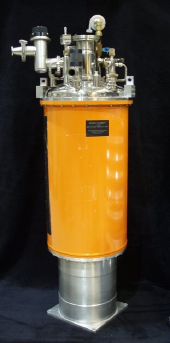
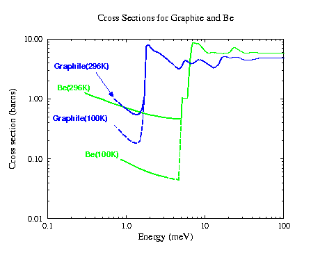
Cite this article
Langel, W. Introduction to neutron scattering. ChemTexts 9, 12 (2023). https://doi.org/10.1007/s40828-023-00184-7
Received:
Accepted:
Published:
DOI: https://doi.org/10.1007/s40828-023-00184-7