
Abstract
This paper represents the exact solution for the properties of the conducting fluid that is flowing past a rotating sphere immersed in a porous medium. It’s a continuation of Sharma and Srivastava (Z Angew Math Mech 103:e202200218, 2022), where the sphere is rotating in the clear fluid region. The solution to the problem was found using Stokes’ equation. In this paper the solutions are found using the Brinkman model in terms of special functions- Bessel’s function of the first and second kind. In this problem, the drag force experienced by the rotating sphere is also calculated for the less permeability of the porous medium. The model is solved using the asymptotic expansion method for the prescribed boundary conditions. By this method, the model consisting of partial differential equations is reduced into ordinary differential equations – modified Bessel’s equations. The results for fluid velocity, stream function, and separation parameters are found in terms of Bessel’s functions and these results match with the existing literature in the absence of Reynolds number. The graphs are plotted for the drag force on the rotating sphere and separation parameter. It has been observed that the separation of the particles occurs at the surface of the sphere more often for high permeability and the drag was found to be decreasing for low permeability. Both graphs were plotted for a range of Reynolds numbers.
1 Introduction
Flow past a body tells about the behavior of fluid as it progresses throughout a body. The fluid interaction with the body can have many outcomes which depend on the properties of the body and of the flow. In the case of the rotating body, the fluid moves around the rotating body, and in this circumstance, the complexity of the model is increased as compared to the stationary body. The rotation of the body can impact the patterns of the flow of the surrounding fluid. When the fluid flows past a rotating body in the presence of a magnetic field, then in that case the study will be influenced by magnetohydrodynamics (MHD).
Underwood (1969) studied fluid flow past a cylinder. He found that the separation parameter takes place at the back of the cylinder for the Reynolds number 5.75. The study was done for the range of Reynolds numbers from the value 0.4–10. Other than separation parameters, other parameters like pressure coefficient, drag coefficient, and streamlines were found and compared positively with the existing literature. Later I Pop (1996) studied the fluid flow past a sphere that is submerged in the permeable medium. For this, he used the Brinkman model. The study was done for the flow separation parameter. It was found for the considered structure that there was no flow separation and in the neighborhood of the sphere there was a velocity surpass. Ovseenko and Ovseenko (1968) considered an incompressible viscid fluid flow around a spinning sphere. The flow parameters were calculated in the series expansion form in terms of Reynolds numbers. The drag on the sphere, pressure, and torque were calculated and it was noticed that the drag on the rotating sphere is higher than the drag on the sphere at rest.
Ghoshal (1970) examined a non-viscous flow past a spheroid and a sphere in the existence of a toroidal magnetic field. In the matter of a sphere, an electric dipole was taken up alongside the axis of symmetry, and in the case of a spheroid, an electric dipole and quadrupole were taken up along the axis of symmetry. It was seen that the expression with flow velocity declined upstream exponentially and downstream algebraically. Few more analyses were done at a far distance of the sphere and also for the area at a far distance of the spheroid. He carried out the work which was done by Ranger (1971). In the work done by Ranger (1971), he considered the presence of the magnetic field. Ranger (1971) noticed that there was an exponential declination of the vorticity in the fluid at every part but leaving the area behind the sphere. In this wake region, the vorticity went off algebraically. Srivastava and Srivastava (2005) examined the flow past a permeable sphere. The model was separated into three sections—inside the permeable sphere, at the interface, and at a distance from the sphere. The equations for the considered model are—Brinkman equation, Stokes and Oseen. The stream function was calculated for the three regions and was matched at the interface. The authors also calculated the drag on the sphere and it was observed that it gets reduced when the considered sphere is porous as well as when the permeability of the sphere was increased. Afterward, both authors (Srivastava and Srivastava 2006) worked on the flow past a permeable sphere a core rigid in nature. Also in this work, three regions were considered which were governed by different equations. The study was done for small Reynolds numbers. The result was found same for the stream function at the interface. The result matched the previous conditions proposed by Ochoa – Tapia, and Whitaker. The drag was found to be increasing with the increase of the ratio of the radii of the concentric spheres and also with the increase in the Darcy number.
Grosan et al. (2010) examined viscous fluid flow past a permeable sphere that is immersed in a porous medium. The investigation was done by the Brinkman model analytically. The streamlines are calculated for the interior and the exterior of the sphere for the distinct values of the porous parameter which rely on the viscosity and the permeableness of both the porous media. The non-dimensional shearing stress was found to be periodic and its magnitude increases on the increment of porous parameters for both the porous media. Satya Deo et al. (2010) considered a model which consists of a fluid sphere which is submerged in a porous medium. The fluid’s movement in the outer region of the fluid sphere was modeled by Brinkman equation whereas the interior of the fluid sphere was by Stokes equation. The drag coefficient was calculated and was found a favorable match with the existing literature. Leont’ev (2014) discussed the fluid’s movement past a sphere and also a cylinder immersed in the permeable medium. Brinkman equation was used to find the exact solution for the no-slip constraints at the interface. The usage of this condition can show the diversity in the flow arrangement near the boundary. Jaiswal and Gupta (2015) considered a problem for which they examined an incompressible viscous flow past a non-miscible Reiner–Rivlin liquid sphere immersed in a porous medium, analytically. Important properties like shear stress and fluid velocity were found on the surface of the considered sphere. They also found similar to Grosan et al. (2010) that dimensionless shear stress is of a periodic nature and its modulus gets reduced along with the permeability parameter. And also this stress remains more or less constant for different values of the considered dimensionless parameter. The separation parameter showed no separation takes place for the considered problem. The drag coefficient was also evaluated. Nurul Farahain Mohammad et al. (2017) examined a problem where boundary layer flow over a sphere in a porous medium is considered unstable. The results for the governing equations were found numerically by the Keller-Box method in the Octave program. The solutions were found for velocity, surface friction, and separation time and it was observed that the porosity can slow down the separation of flow and increase the velocity at frontal and back stagnation points. The shear stress dominates the turnaround of the flow. Madasu et al. (2021) studied the fluid’s slow movement past a spheroid in a porous medium. The slip flow boundary conditions were considered at the interface. In this problem, prolate and oblate spheroids were examined. The drag was found analytically and was seen as its dependence on permeability, and deformity. The outcomes of slip have seen exceptional effects in the case of increasing drag. The different models for which fluid properties were discussed are studied in the papers (Kumar et al. 2016; Maneesha et al. 2017; Singh et al. 2019; Varghese and Jayakumar 2017; Narayanan et al. 2021). These models can be associated with atmospheric problems and also geo-dynamo.
Sharma and Srivastava (2021) examined the variety of fluid quantities for the fluid that is flowing in the annular region made up by using two spheres that were rotating with different velocities in the existence of the toroidal magnetic field. It was noticed that the impact of rotation is better in the first estimation of the velocity. It was also observed that the stream function was reversely proportionate to the magnetic parameter but this parameter didn’t have any impact on the velocity. Shreen El-Sapa and Noura S. Alsudais (2021) considered the flow which is generated by two spheres immersed in a porous medium. Both spheres are of different sizes and moving translatory with different velocities. The hydrodynamic drag was found for both the sphere which coincides with several values of Hartmann number and permeability parameter. These numbers indicate the magnetic field’s presence; the separation parameter, porosity, velocity, and the ratio of the size of both spheres respectively. Saad (2021) looked into the impact of Magnetic regions on an incompressible viscous fluid flow. The fluid is flowing past a porous sphere and it is kept in a spherical cell and they are not concentric. The Brinkman equation is the governing equation for the porous sphere and the spherical shell with clear fluid is governed by the Stokes equation. The problem is solved for the different values of the Hartmann numbers. The drag, which is hydrodynamic in nature was found on the porous sphere numerically. The streamlines were seen all over the porous media for the Happel and Kuwabara unit cell models at distinct values of applicable parameters.
A toroidal magnetic field is attributed to a magnetic field that is similar to the shape of a torus. This torus is similar to a doughnut. This magnetic field is frequently experienced in many physical and engineering problems. Both the poloidal and toroidal components of the field are important. The toroidal component of the Earth’s magnetic field plays a very important role in the dynamics of the geodynamo. This component develops and preserves the earth’s magnetic field.
In this paper, the effect of the toroidal magnetic field is investigated for the fluid flow past a rotating solid sphere immersed in a porous medium. The purpose of this work is to show an analytical explanation of the fluid properties of the flow past a rotating solid sphere. We have found an approximated solution through the perturbation technique. The results are shown through graphs.
2 Problem
The problem consists of a rotating sphere that is immersed in a porous media (Fig. 1). The conducting fluid flow past this sphere is examined. The stream velocity is uniform at infinity. The radius of the sphere is a.

Schematic diagram of the stated problem
2.1 Mathematical modeling of the stated problem
The fluid is flowing with the velocity q for the linear and rotating motion in the cylindrical polar coordinates \(\left(w,\phi ,z\right)\) given as follows:
With the toroidal magnetic field, with no component in the direction of the radius
Here \(q_{z}\) and \(q_{w}\) are the velocity’s components along with the unit vectors \(\hat{e}_{z}\) and \(\hat{e}_{w}\) respectively, and given as follows:
And \(w = r\sin \theta\) and \(z = r\cos \theta\) are considered in the spherical polar coordinate system.
The vector form of the governing equation, taken up from Srivastava and Srivastava (2005) with some modification due to the presence of magnetic is defined as follows:
Here J: current density and \(\mu_{0} J = \nabla \times B_{T} .\)
3 Boundary conditions
The conditions for the governing equation are described as follows:
Non-dimensional quantities are defined as follows:
Here \(\zeta\): Taylor number and \({\text{Re}}\): Reynolds number.
The boundary conditions in dimensionless form can be written as follows:
Boundary conditions are considered at the interface and also far from the rotating sphere. Since the sphere is solid so the velocity at surface of the sphere is taken as zero. The governing equations in non dimensionalized form are as follow:
where \( D^{2} \equiv \frac{{\partial^{2} }}{{\partial z^{2} }} + \frac{{\partial^{2} }}{{\partial w^{2} }} - \frac{1}{w}\frac{\partial }{\partial w},\;\gamma^{2} = \frac{{\mu_{e} }}{\mu },\;{\text{and}}\;c = \frac{a}{{\gamma \sqrt {\rm K} }}\) is a Darcy number.
Figure 1 illustrates the stated problem. It shows the fluid flow past a rotating solid sphere. The toroidal magnetic field’s presence is being taken in this model.
4 Analytic solutions
The properties of fluid—velocity and stream function are considered as an expansion in the terms of \({\text{Re}}\) as follows:
4.1 First approximation
Substituting the expansion (4.1a) in Eq. (3.5), and equating the terms independent of \({\text{Re}} ,\) we get the following equation.
This assumption for the fluid velocity for the fluid flow past a rotating sphere is a simplified form of velocity. This assumption has only the radial component which provides an easy model although representing some of the effects of rotation.
Substituting the assumption (4.2b) in Eq. (4.2a), we get the modified Bessel’s equation as follows:
The solution of (4.3a) can be written as follows:
where \( I_{{{\raise0.7ex\hbox{$3$} \!\mathord{\left/ {\vphantom {3 2}}\right.\kern-0pt} \!\lower0.7ex\hbox{$2$}}}} \left( {rc} \right) = \sqrt {\frac{2}{\pi rc}} \left( {\cosh rc - \frac{\sinh rc}{{rc}}} \right),\) and \(K_{{{\raise0.7ex\hbox{$3$} \!\mathord{\left/ {\vphantom {3 2}}\right.\kern-0pt} \!\lower0.7ex\hbox{$2$}}}} \left( {rc} \right) = \sqrt {\frac{\pi }{2rc}} e^{ - rc} \left( {1 + \frac{1}{rc}} \right).\)
By boundary condition (3.3c), the first estimation for fluid velocity is found as follows:
\({\text{where}} \;C_{1} = 0 \;{\text{and}}\;C_{2} = \frac{1}{{\sqrt c K_{{{\raise0.7ex\hbox{$3$} \!\mathord{\left/ {\vphantom {3 2}}\right.\kern-0pt} \!\lower0.7ex\hbox{$2$}}}} \left( c \right)}} \).
Now substituting the expansion (4.1b) in Eq. (3.4), we get the following equation, independent of \(R_{e}\)
Assume the following form for \(\psi_{0}\):
Substituting the (4.6b) in Eq. (4.6a) can be rewritten as:
Equation (4.7a) is a modified Bessel’s equation, whose solution is given as follows:
Equation (4.7b) can be written as follows:
The solution of Eq. (4.8a) is given as follows:
The constant \({{\text{A}}}_{0}\) which make the stream function infinite is considered zero.
For evaluating the remaining constants of integration, consider (3.3a) for (4.8b), we get the solution of stream function as follows:
The solution exactly goes with the result found by Pop (1996) for \({\psi }_{0}\).
It is noticed that the first estimation matches with the condition (3.1a) as \(r\to \infty \) and for large c i. e. in this stream function can be written as:
4.2 Second approximation
The second estimation for the solution in the exterior area of the rotating sphere is found using the recommended boundary conditions. The terms which are dependent on \({\text{Re}}\) of order 1 after substituting the expansion (4.1a) in the Eq. (3.5), give the following equation
Assuming the following form for \(V_{1}\) suggested by equation (Vasudeviah and Malathi 1995)
Substituting the above assumption in Eq. (4.10a), the LHS gives the following term
The coefficient of \(\left( {1 - \eta^{2} } \right)\) of the Eq. (4.10a) give the following equation.
The solution of Eq. (4.11a), which is a modified Bessel’s equation is given as follow:
And also the coefficient of \(\eta \left( {1 - \eta^{2} } \right)\) of the Eq. (4.10a) is given by
where \(H_{1} = \frac{1}{2}\left( {1 + \frac{{3K_{{{\raise0.7ex\hbox{$3$} \!\mathord{\left/ {\vphantom {3 2}}\right.\kern-0pt} \!\lower0.7ex\hbox{$2$}}}} \left( c \right)}}{{cK_{{{\raise0.7ex\hbox{$1$} \!\mathord{\left/ {\vphantom {1 2}}\right.\kern-0pt} \!\lower0.7ex\hbox{$2$}}}} \left( c \right)}}} \right).\)
The homogeneous solution of Eq. (4.12a), which is non – homogeneous modified Bessel’s equation, is given as follow:
where
The solution is obtained only for homogeneous form because of large c.
Therefore,
After using boundary condition in Eq. (4.12c) defined for \({V}_{1}\) as follow:
Gives the result for the fluid velocity, which can be written as follows:
The terms which are dependent on \({\text{Re}}\) of order 1 after substituting the expansion (4.1b) in the Eq. (3.4), give the following equation
Assuming \(\psi_{1}\) in the following form:
This assumption for the stream function involves the influence of the rotating sphere on the fluid flow and also upholding the complexity of the model.
The LHS of (4.14) leads to
where \(\chi_1=G^{\prime\prime} (r)-2/r^2 G(r)\) and \(\chi_2=H^{\prime\prime} (r)-6/r^2 H(r)\)
The Eq. (4.14) takes the following form:
The solution of (4.16a) is written as follow:
Which is a non – homogeneous Cauchy’s Euler equation whose solution is given by,
After using the boundary conditions (3.3a) and (3.3b), the solution (4.17b) after assuming L1 and A3 zero, is given as follow:
where \({\text{B}}_{3}\) is an arbitrary constant.
The solution of (4.16b) can be written as follows:
where \(\left( {\chi_{2} } \right)_{p}\) is the particular integral of (4.16b).
Due to the complexity of solution to the Eq. (4.16b), only the homogeneous part is considered.
After using the conditions (3.3a) and (3.3b) in (4.18a), the solution (4.18b) after assuming L2 and A4 zero, is given as follow:
where \({{\text{B}}}_{4}\) is an arbitrary constant.
Therefore, the stream function is given by,
It is noticed that the stream function is not influenced by the magnetic parameter at this level as well.
Hence the stream function (4.1b) can be written as follows:
\({\text{B}}_{3}\) and \({\text{B}}_{4}\) are considered as 1 for the simplicity of the form (4.20a). Hence
The stream function \(\psi =0\) at r = 1. So, there are no stream lines on the surface of the sphere.
5 Result and discussions
5.1 Separation parameter
The dimensionless vorticity is calculated for the outer region of the sphere. This parameter examines the separation of fluid from the surface of the sphere.
As stated by Underwood (1969), the separation parameter SEP is given as follows:
The separation parameter matches with the result given by I Pop (1996) for \({\text{Re}} = 0.\)
The tangential velocity can be found as follows:
The above expression, at the boundary of the sphere r = 1 is
5.2 Drag on the rotating sphere
To calculate the drag force on the rotating sphere, normal stress and the shear stress are found by using the following form in spherical coordinates, respectively
For large c, we have very less permeability and in that case the pressure on the sphere due to the fluid flow in porous medium is considered negligible.
Therefore, the components of stress tensor for r = 1 are given as follows:
where \(q_{r} = \frac{1}{{r^{2} \sin \theta }}\frac{\partial \psi }{{\partial \theta }}\) and \(q_{\theta } = - \frac{1}{r\sin \theta }\frac{\partial \psi }{{\partial r}}\) are the components of velocity in the direction of unit vectors \(\hat{e}_{r}\) and \(\hat{e}_{\theta }\) respectively in the spherical coordinates system.
The drag force on the surface of sphere is found using the following formula:
This drag force is calculated for the case when permeability of the medium is less i.e.\(\mathrm{\rm K} \to 0.\)
6 Discussion of different cases and conclusions
6.1 Three possible cases of rotating spheres
Our investigation is led by the following cases:
6.1.1 Case 1: slow flow past a rotating sphere
Ranger (1971) investigated the slow flow past a rotating sphere. The primary Stokes flow past a non-rotating sphere together with an antisymmetric secondary flow in the azimuthal plane induced by the spinning sphere were studied. He found that in the azimuthal plane a region of reversed flow attached to the rear portion of the sphere is seen.
The structure of the vortex is described and is shown to be confined to the rear portion of the sphere. In this case the eddies were observed only for the rear region of the sphere for \(R_{o}^{2} > 6 {\text{Re}}\).
Whereas the case discussed by Majhi and Vasndevaiah (1982) for viscous parabolic shear flow past a spinning sphere for low Reynolds number, the eddies are seen in rear or front or both areas of the sphere for the distinct values of uniform stream, and the ratio of \(R_{o}^{2} {\text{and}} {\text{Re}}\) where \(R_{o}\) is rotational Reynolds number and \({\text{Re}}\) is Reynolds number.
The physical drag was also found and given as follows:
It was observed that in the non – appearance of unform stream, the ratio of pressure drag and skin-friction drag is 1:2 and also the drag was seen to be vanished when uniform stream is 2/3.
In the absence of inertia term in the Navier–Stokes equations converts into Stokes flow, which describes viscous-dominated fluid flow. Castillo et al. (2019) examined the effect of the rotation on the drag. The study was done numerically and experimentally. They wanted to give further proofs for the changes in the drag because of the rotation of the sphere in the absence of fluid inertia. It was seen that the drag on the sphere in a viscoelastic fluid was getting decreased on the increment of the rotation of the sphere and also due to elastic effects there was an increment in the settling velocity. In the non-inertia stage, the drag was reduced at O(Wi2) for small values of De and Wi. Here De is Deborah Number, and Wi is rotational Weissenberg number.
6.1.2 Case 2: slow flow past a rotating sphere in Brinkman medium
Solomentsev and Anderson (1996) considered the case where a sphere is rotating in the Brinkman medium. It was observed that the effect of the Brinkman term was very less on the rotational motion as compared to translation motion. The drag force in the porous medium in connection with Newtonian fluid is (given) considered. The proportion of diffusion terms in the the Brinkman medium to the Newtonian fluid comes as a reciprocal to the ratio of drag forces. Also since the Brinkman term has a different impact on the rotation of the sphere, so the ratio of diffusion due to rotation of the sphere depends in a different way on \(a/\sqrt{k}\). The torque in the Brinkman medium in connection with Newtonian fluid is found as an expansion in terms of small \(a/\sqrt{k}\).
In the case of neglecting inertia term from the governing equation i.e., Brinkman equation gives rise to Darcy’s law, which represents the flow through porous medium typically for low Reynolds number. In such situation, the eddies, vortices are not being considered. Vasudeviah and Malathi (1995) considered a model in which slow viscous fluid was flowing past a spinning sphere with the permeable surface. They calculated the drag coefficient and showed the correction in the existing literature for the same. This drag coefficient follows the collective outcome of rotation and permeability for very small values of Re (< 1). In the case of porous structure, the drag seems to be reduced as compared to the case with an identical solid body.
6.1.3 Case 3: slow flow past a rotating sphere in the presence of the toroidal magnetic field
Sharma and Srivastava (2022) considered the model which consists of slow flow past a rotating sphere in the presence of the toroidal magnetic field.
They studied the separation phenomena evoked due to the rotation of a solid sphere. The whole process is modeled in terms of a partial differential equation and solved using the perturbation method. The following conclusion is being made during the study:
-
1.
The expression for the first approximation of velocity is same as that of Ranger. This shows that there will not be any impact on the velocity due to the magnetic field.
-
2.
The expression for the first approximation of stream function is also the same as that of Ranger, confirming zero impact of the magnetic field.
-
3.
In the limit of r → ∞., the first approximation solution converges to the first term of Oseen’s solution.
-
4.
Also, it has been observed that the second approximate solution, for the region outside the sphere, is similar to the second approximation of the velocity seen in Ranger’s solution.
-
5.
The graph of separation phenomena occurring at the surface of the sphere. It has been observed that the separation of particles occurs more frequently for the low rotation parameter as compared to the high value of the rotation parameter.
-
6.
We have plotted the graph of separation phenomena occurring at the surface of the sphere. It has been observed that the separation of particles occurs more frequently for the high magnetic field as compared to the lesser value of the magnetic field. This may be because Lorentz’s force generated due to the magnetic field is trying to retard the velocity of flow particles.
-
7.
The angle with which the upstream strikes the surface of the sphere and the downstream angle with which it exits the surface of the sphere is given various values of the Taylor number. It shows that with an increase in Taylor number, there is an increase in the angle of exit, but the angle of entry will decrease.
Hence, overall, the impact of the magnetic field and the rotation is visible in the flow field.
Chakraborty (1963) considered the conducting fluid flow past a rotating sphere which conducting magnetized. The toroidal magnetic field is produced due to the rotation of the sphere and its velocity component disappear as approaches to stagnation point.
The rotation of the sphere doesn’t impact drag experienced by the sphere. Also the torque was found which opposes the rotation of the sphere and is proportional to the angular velocity of the sphere. This torque was also depending on the magnetic property of the body.
Zhang and Fearn (1994) investigated the instabilities of the field in the case of rotating spherical shells in the presence of toroidal magnetic field. The study for the instabilities is being done in the presence and absence of inertia.
It was found that there was no change in the main characteristics of the instabilities even after neglecting inertia term when Tm > 105 (Tm: Magnetic Taylor number).
6.2 Conclusions
The intention behind this paper is to study the drag force due to the fluid flow, experienced by a rotating solid sphere in the magnetic field’s existence. And also, the separation parameter awakens because of the rotating solid sphere. The mathematical model consists of partial differential equations, later converted in a set of ordinary differential equations and solved analytically. The following conclusions are found:
-
1.
The first approximation of the stream function (4.9a) is similar to the result found by I Pop. Here, no influence of the magnetic parameter is seen. The result matches with the considered boundary condition (3.1b) for r →∞.
-
2.
The expression for the separation parameter depending on first estimation of the stream function (4.9a) is similar to the result found by I Pop, which is given in (5.2b), the term independent of Re. Here also, there is no impact of the magnetic field is seen.
-
3.
The drag force (5.6b) on the surface of the rotating sphere is calculated for the low permeability of the porous medium. With the assumption that there is no pressure of the fluid on the sphere due to low permeability (Fig. 2).
Fig. 2 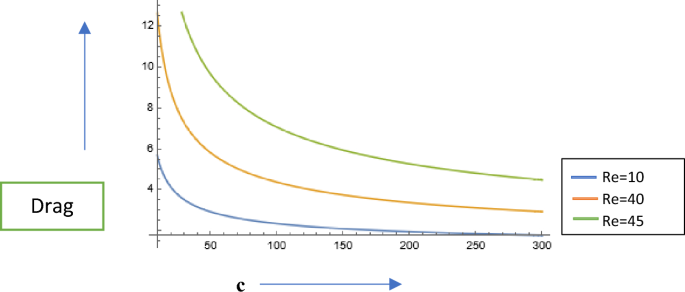
Graph of drag versus c \(\left( {\alpha \frac{1}{{{\text{permeability}} \,\;{\text{parameter}}}}} \right)\)
-
4.
The Fig. 3 represents the graph for the separation parameter that appears at the surface of the rotating sphere. The separation of the particles was seen more for high permeability of the medium than the low permeability in the range of Reynolds number (10 < Re < 60).
Fig. 3 
Graph of separation parameter versus c \(\left( {\alpha \frac{1}{{\text{permeability parameter}}}} \right)\)
-
5.
The Fig. 2 represents the graph for the drag force which is experienced by the surface of the rotating sphere. The drag force is seen to be deteriorating for low permeability of the medium in the range of Reynolds number (10 < Re < 45).
-
6.
The impact of Taylor’s number is not seen in the solution because the results are found for less permeability which was making the solution independent of Taylor number. In case of large permeability, the problem becomes more complex and finding the analytic solution is more complicated. However, in that case the solutions for fluid properties depend on Taylor number.


Abbreviations
- V :
-
Flow velocity
- Ψ :
-
Stream function
- μ :
-
Dynamic viscosity
- \({\mu }_{e}\) :
-
Effective viscosity
- Re:
-
Reynolds number
- \({B}_{T}\) :
-
Toroidal magnetic field
- c :
-
Darcy’s number
- \(\zeta \) :
-
Taylor number
- J :
-
Current density
- \(\Omega \) :
-
Angular velocity
- ρ :
-
Density
- K :
-
Permeability
- \({\mu }_{0}\) :
-
Magnetic permeability
References
Anirudh Narayanan, B., Lakshmanan, G., Mohammad, A., Ratna Kishore, V.: Laminar flow over a square cylinder undergoing combined rotational and transverse oscillations. J. Appl. Fluid Mech. 14(1), 259–273 (2021)
Castillo, A., Murch, W.L., Einarsson, J., Mena, B., Shaqfeh, E.S.G., Zenit, R.: Drag coefficient for a sedimenting and rotating sphere in a viscoelastic fluid. Phys. Rev. Fluids 4, 063302 (2019)
Chakraborty, B.B.: Flow of a conducting fluid past a rotating magnetized sphere. J. Indian Inst. Sci. 45, 1 (1963)
Deo, S., Shukla, P., Gupta, B.R.: Drag on a fluid sphere embedded in a porous medium. Adv. Theor. Appl. Mech. 3(1), 45–52 (2010)
El-Sapa, S., Alsudais, N.S.: Effect of magnetic field on the motion of two rigid spheres embedded in porous media with slip surfaces. Eur. Phys. J. E 44, 68 (2021)
Ghoshal, S.: Flow past spheres and spheroids in the presence of a toroidal magnetic field. Pre Appl. Geophys. 81, 223–229 (1970)
Grosan, T., Postelnicu, A., Pop, I.: Brinkman flow of a viscous fluid through a spherical porous medium embedded in another porous medium. Transp Porous Med. 81, 89–103 (2010)
Jaiswal, B.R., Gupta, B.R.: Brinkman Flow of a Viscous Fluid Past a Reiner-Rivlin Liquid Sphere Immersed in a Saturated Porous Medium. Springer, Dordrecht (2015)
Kumar, S., Rangan, P.V., Ramesh, M.V.: Poster: pilot deployment of early warning system for landslides in eastern Himalayas. In: Proceedings of the Annual International Conference on Mobile Computing and Networking, MOBICOM, vol. 03-07-October-2016, pp. 97–108. (2016)
Leont’ev, N.E.: Flow past a cylinder and a sphere in a porous medium within the framework of the Brinkman equation with the Navier boundary condition. Fluid Dyn. 49(2), 232–237 (2014)
Madasu, M.K., Bucha, T.: Slow motion past a spheroid implanted in a Brinkman medium: slip condition Krishna Prasad. Int. J. Appl. Comput. Math 7, 162 (2021)
Majhi, S.N., Vasndevaiah, M.: Flow separation in a viscous parabolic shear past a sphere. Acta Mech. 45, 233–249 (1982)
Mohammad, N.F., Waini, I., Kasim, A.R.M., Majid, N.A.: Unsteady Boundary layer flow over a sphere in a porous medium. AIP Conf. Proc. 1870, 040076 (2017)
Ovseenko, R.I., Ovseenko, Yu.G.: Drag Of A Rotating Sphere. Izv. AN SSSR. Mekhanika Zhidkosti i Gaza 3(1), 110–118 (1968)
Pop, I., Ingham, D.B.: Flow past a sphere embedded in a porous medium based on the Brinkman model. Int. Commun. Heat Mass Transf. 23(6), 865–874 (1996)
Ramesh, M.V., Pullarkatt, D., Geethu, T.H., Rangan, V.P.: Wireless sensor networks for early warning of landslides: experiences from a decade long deployment. In: Advancing Culture of Living with Landslides. Springer, Cham (2017)
Ranger, K.B.: Slow viscous flow past a rotating sphere. In: Mathematical Proceedings of the Cambridge Philosophical Society, POPS, vol. 69, pp. 63–36. (1971)
Saad, E.I.: Magnetic fields effect on a porous sphere in a nonconcentric spherical cell. J. Porous Media 24(4), 1–18 (2021)
Sharma, B., Srivastava, N.: Fluid flow in between the differentially rotating spherical shells in the presence of toroidal magnetic field. In: Proceedings of the ASME 2021, Copyright © 2021 by ASME
Sharma, B., Srivastava, N.: Fluid flow past a rotating sphere in the presence of a toroidal magnetic field. Z. Angew. Math. Mech. 103, e202200218 (2022)
Singh, P., Velamati, R.K., Prathap, C., Mohammad, A., Chander, S.: Study of flow patterns and impingement heat transfer for an annular array of eight C-rotating Dual-swirling flames. Int. J. Heat Mass Transf. 144, 118657 (2019)
Solomentsev, Y.E., Anderson, J.L.: Rotation of a sphere in Brinkman fluids. Phys. Fluids 8, 1119 (1996)
Srivastava, A.C., Srivastava, N.: Flow past a porous sphere at small Reynolds number. Z. Angew. Math. Phys. 56, 821–835 (2005)
Srivastava, A.C., Srivastava, N.: Flow of a viscous fluid at small Reynolds number past a porous sphere with a solid core. Acta Mech. 186, 161–172 (2006)
Underwood, R.L.: Calculation of incompressible flow past a circular cylinder at moderate Reynolds numbers. J. Fluid Mech. 37(1), 95–114 (1969)
Varghese, J., Jayakumar, J.S.: Numerical investigation of flow parameters for solid rigid spheroidal particle in a pulsatile pipe flow. IOP Conf. Ser. Mater. Sci. Eng. (online) 243(1), 8 (2017). https://doi.org/10.1088/1757-899X/243/1/012008
Vasudeviah, M., Malathi, V.: Slow viscous flow past a spinning sphere with permeable surface. Mech. Res. Commun. 22(2), 191–200 (1995)
Zhang, K., Fearn, D.R.: Hydromagnetic waves in rapidly rotating spherical shells generated by magnetic toroidal decay modes. Geophys. Astrophys. Fluid Dyn. 77, 133–157 (1994)
Acknowledgements
The work in this paper would not have been done without the constant support of the committee members and Amrita School of Engineering, Bangalore. The authors show their gratitude for the constant encouragement of the committee.
Funding
Work is done in the Lab VGST-GRD787.
Author information
Authors and Affiliations
Corresponding author
Ethics declarations
Conflict of interest
Authors have no conflict of interest.
Ethical approval
Authors with significant contribution are appropriately acknowledged and included. The manuscript is not submitted or published anywhere.
Additional information
Publisher's Note
Springer Nature remains neutral with regard to jurisdictional claims in published maps and institutional affiliations.
Rights and permissions
Springer Nature or its licensor (e.g. a society or other partner) holds exclusive rights to this article under a publishing agreement with the author(s) or other rightsholder(s); author self-archiving of the accepted manuscript version of this article is solely governed by the terms of such publishing agreement and applicable law.
About this article

Cite this article
Sharma, B., Srivastava, N. Study of toroidal magnetic field for the flow past a rotating rigid sphere embedded in the less permeable medium. Int J Geomath 15, 5 (2024). https://doi.org/10.1007/s13137-024-00246-z
Received:
Accepted:
Published:
DOI: https://doi.org/10.1007/s13137-024-00246-z