Configuration optimization for heterogeneous time-sensitive networks

Abstract

Time-Sensitive Networking (TSN) collectively defines a set of protocols and standard amendments that enhance IEEE 802.1Q Ethernet nodes with time-aware and fault-tolerant capabilities. Specifically, the IEEE 802.1Qbv amendment defines a timed-gate mechanism that governs the real-time transmission of critical traffic via a so-called Gate Control List (GCL) schedule encoded in each TSN-capable network device. Most TSN scheduling mechanisms are designed for homogeneous TSN networks in which all network devices must have at least the TSN capabilities related to scheduled gates and time synchronization. However, this assumption is often unrealistic since many distributed applications use heterogeneous TSN networks with legacy or off-the-shelf end systems that are unscheduled and/or unsynchronized. We propose a new scheduling paradigm for heterogeneous TSN networks that intertwines a network calculus worst-case interference analysis within the scheduling step. Through this, we compromise on the solution’s optimality to be able to support heterogeneous TSN networks featuring unscheduled and/or unsynchronized end-systems while guaranteeing the real-time properties of critical communication. Within this new paradigm, we propose two solutions to solve the problem, one based on a Constraint Programming formulation and one based on a Simulated Annealing metaheuristic, that provide different trade-offs and scalability properties. We compare and evaluate our flexible window-based scheduling methods using both synthetic and real-world test cases, validating the correctness and scalability of our implementation. Furthermore, we use OMNET++ to validate the generated GCL schedules.

1 Introduction

Real-time communication with safety guarantees over standardized protocols is becoming increasingly necessary in various application domains, such as industrial automation and advanced driver assistance in automotive applications (Ashjaei et al. 2021). Time-Sensitive Networking (TSN) (Institute of Electrical and Electronics Engineers 2016a) is a collection of amendments and protocols that enhances standard 802.1 Ethernet to provide real-time capabilities such as time synchronization, preemption, redundancy management and scheduled traffic (Craciunas et al. 2016). Through TSN, safety-critical scheduled traffic (ST) can be isolated and guaranteed in the presence of best-effort (BE) traffic within the same multi-hop switched Ethernet network. The main TSN mechanisms that enable ST traffic with bounded latency and jitter to coexist with BE communication are a network-wide clock synchronization protocol [802.1ASrev (Institute of Electrical and Electronics Engineers 2017] and a Time-Aware Shaper (TAS) mechanism (Institute of Electrical and Electronics Engineers 2016b) with a global communication schedule implemented in Gate Control Lists (GCLs). The TAS mechanism operates as a gate for each transmission queue, allowing or denying the transmission of frames as configured in the GCL schedule.

Most previous work guaranteeing real-time communication behavior through TSN networks (e.g., Craciunas et al. 2016; Serna Oliver et al. 2018; Pop et al. 2016) assume that the network devices are homogeneous, i.e., they all have the time-aware gating mechanism and are synchronized to a global network time. However, many brownfield deployments in industrial systems require end-to-end guarantees in heterogeneous TSN networks that connect TSN-capable switches with legacy resource-constrained end-points (e.g., PLC, sensors, actuators) that are not easily retrofitted with TSN capabilities. Moreover, in industrial systems that have a long life-cycle and which are dependent on legacy technology (Schriegel et al. 2018), customers are more likely to accept the replacement of switches but not of customized end-points; hence it is more beneficial to transition gradually to new technologies making the integration of legacy systems into TSN networks essential (Mateu et al. 2021). Furthermore, converged IT/OT networks in, e.g., fog and edge use-cases (Schriegel et al. 2018), interconnection of TSN networks with, e.g., 5G domains (Larrañaga et al. 2020), or multi-domain TSN networks with different sync mechanisms cannot readily communicate isochronous (fully periodic) traffic (Böhm and Wermser 2021). Here, the region outside the TSN domain can be viewed as an unscheduled and unsynchronized end-point sending sporadic critical traffic. Moreover, even if the end-points do have some form of TSN capability (e.g., via switched end-points, von Arnim et al. 2020), the software layers on top of the TSN hardware mechanism can suffer from non-deterministic jitter and delays, leading to missed transmission slots and ultimately resulting in a sporadic, rather than periodic frame transmission from the end-points.

Hence, we investigate heterogeneous TSN networks in which end-systems are unscheduled and/or unsynchronized, meaning that they do not have TSN capabilities (such as 802.1Qbv and 802.1AS) and thus lead to sporadic arrivals of critical traffic at the TSN-capable switches or domains. Classical schedule generation methods for GCLs typically enforce either a fully deterministic, 0-jitter forwarding of critical frames with exact SMT/ILP-based solvers (Craciunas et al. 2016) or heuristics (Pop et al. 2016), or a more flexible window-based approach that allows a bounded interference between critical frames (Serna Oliver et al. 2018). The drawback of these methods is that they require end-systems to send critical frames in a scheduled and synchronized way that matches the forwarding schedule of switches, and thus necessitate TSN capabilities in both end systems and switches. Other work, cf. Reusch et al. (2020), Hellmanns et al. (2020a), introduce scheduling approaches that do not impose synchronization on the end-systems level but constrain all forwarding GCL windows on switches to be aligned and, in the case of Hellmanns et al. (2020a), do not use safe formal verification methods like network calculus for the interference calculation used for the schedule creation.

In this paper, which is an extended version of Barzegaran et al. (2022), we consider heterogeneous TSN networks, relaxing the requirement that end-systems need to be synchronized and/or scheduled and, furthermore, take into account relative offsets of windows on different nodes. We intertwine the worst-case delay analysis from Zhao et al. (2020) with the scheduling step in order to generate correct schedules where the end-to-end requirements of ST streams (also called flows in previous work) are met. Furthermore, we compare different TSN scheduling approaches that have been proposed in the literature (see Table 3 for an overview) to our flexible window-based approach. We define the analysis-driven window optimization problem resulting from our more flexible approach with the goal to be able to enlarge the solution space, reduce computational complexity, and apply it to end-systems without TSN mechanisms. Depending on industrial applications’ requirements, our evaluation can help system designers choose the most appropriate combination of configurations for their use-case. The main contributions of the paper are:

• We propose a novel flexible window-based scheduling method that does not individually schedule ST frames and streams, but rather schedules open gate windows for individually scheduled queues. Hence, we can support non-deterministic queue states and thus networks with unscheduled and/or unsynchronized end-systems by integrating the WCD Network Calculus (NC) analysis into the scheduling step. The NC analysis is used to construct a worst-case scenario for each stream to check its schedulability, considering arbitrary arrival times of these streams and the given open GCL window placements.

• We formulate the “window optimization problem” and provide timing guarantees for real-time streams even in systems with unscheduled and unsynchronized end systems.

• We propose two solutions to solve the problem, one based on a Constraint Programming formulation and one based on a Simulated Annealing (SA) metaheuristic.

• For the CP formulation, we propose a proxy function as an alternative to the network calculus analysis in Zhao et al. (2020) and use it to provide timing guarantees inside the CP search.

• We compare and evaluate our flexible window-based scheduling method with existing scheduling methods for TSN networks. The evaluation is based on both synthetic and real-world test cases, validating the correctness and the scalability of our implementation. Furthermore, we use the OMNET++ simulator to validate the generated solutions.

We start by introducing the system, network, and application models in Sect. 2 and outline the problem formulation, including a motivational example, in Sect. 3. In Sect. 4, we present the novel scheduling mechanism and the optimization strategy based on Constraint Programming (CP), followed by our heuristic solution in Sect. 5. We review related research in Sect. 6, focusing on the existing scheduling mechanisms that we compare our work to. In Sect. 7, we present the comparison and evaluation results of our methods and conclude the paper in Sect. 8.

2 System model

This section defines our system model for which we summarize the notation in Table. 1.

Table 1 Summary of notations

2.1 Network model

We represent the network as a directed graph $G=(\varvec{V,E})$ where $\varvec{V}=\varvec{ES}\bigcup \varvec{SW}$ is the set of end systems (ES) and switches (SW) (also called nodes), and $\varvec{E}$ is the set of bi-directional full-duplex physical links. An ES can receive and send network traffic while SWs are forwarding nodes through which the traffic is routed. The edges $\varvec{E}$ of the graph represent the full-duplex physical links between two nodes, $\varvec{E}\subseteq \varvec{V}\times \varvec{V}$. If there is a physical link between two nodes $v_a, v_b\in \varvec{V}$, then there exist two ordered tuples $[v_a, v_b], [v_b,v_a]\in \varvec{E}$. An equivalence between output ports $p\in P$ and links $[v_a,v_b]\in \varvec{E}$ can be drawn as each output port is connected to exactly one link. A link $[v_a, v_b]\in \varvec{E}$ is defined by the link speed C (Mbps), propagation delay $d_p$ (which is a function of the physical medium and the link length), and the macrotick mt. The macrotick is the length of a discrete time unit in the network, defining the granularity of the scheduling timeline (Craciunas et al. 2016). Without loss of generality, we assume $d_p=0$ in this paper.

As opposed to previous work, we do not require that end-system are either synchronized or scheduled. Since ESs can be unsynchronized and unscheduled, they transmit frames according to a strict priority (SP) mechanism. Switches still need to be synchronized and scheduled using the 802.1ASrev and 802.1Qbv, respectively. Please note that our method also works for systems where only a subset of the ESs are unsynchronized or unscheduled, and the rest have TSN capabilities. However, in such mixed systems, the response times of critical traffic coming from synchronized/scheduled ESs may be unnecessarily pessimistic, and the pessimism may lead to reduced schedulability in some use cases. If schedulability needs to be increased and the pessimism decreased, we need to isolate critical traffic that arrives at a switch from TSN-capable ESs from any other traffic. This can be achieved by placing the scheduled critical traffic from scheduled and synchronized ESs into different queues than the sporadic traffic arriving from unscheduled/unsynchronized ESS in order to eliminate interference. While this will guarantee a deterministic timely behavior as in the classical models (e.g. Craciunas et al. 2016; Serna Oliver et al. 2018), it will mean that the reserved queues will not be available for the sporadic critical traffic arriving from unscheduled/unsynchronized ESs.

2.2 Switch model

Figure 1a depicts the internals of a TSN switch. The switching fabric decides, based on the internal routing table to which output port p a received frame will be forwarded. Each egress port has a priority filter that determines in which of the available 8 queues/traffic-classes $q\in p \cdot Q$ of that port a frame will be put. We assume that all 8 may (but don’t have to) be used. Within a queue, frames are transmitted in first-in-first-out (FIFO) order. Similar to Craciunas et al. (2016), a subset ($p \cdot Q_{ST}$) of the queues is reserved for ST traffic, while the rest ($p \cdot \overline{Q}$) are used for non-critical communication. As opposed to regular 802.1Q bridges, where enqueued frames are sent out according to their respective priority, in 802.1Qbv bridges, there is a TAS, also called timed-gate, associated with each queue and positioned behind it. A timed-gate can be either in an open (O) or closed (C) state. When the gate is open, traffic from the respective queue is allowed to be transmitted, while a closed gate will not allow transmission, even if the queue is not empty. When multiple gates are open simultaneously, the highest non-empty priority queue gets selected first, blocking others until it is empty or the corresponding gate is closed. The 802.1Qbv standard includes a mechanism to ensure that no frames can be transmitted beyond the respective gate’s closing point. This look-ahead checks whether the entire frame present in the queue can be fully transmitted before the gate closes and, if not, it will not start the transmission.

Fig. 1

TSN Switch model and queue interference

The state of the queues is encoded in a GCL, which (contrary to e.g., TTEthernet Issuing Committee 2011) acts on the level of traffic-classes instead of on an individual frame level (Craciunas and Serna Oliver 2017). Hence, an imperfect time synchronization, frame loss, ingress policing (cf. Craciunas et al. 2016), or the variance in the arrival of frames from unscheduled and/or unsynchronized ESs may lead to non-determinism in the state of the egress queues and, as a consequence, in the whole network. If the state of the queue is not deterministic at runtime, the order and timing of the sending of ST frames can vary dynamically. In Fig. 1b, the schedule for the queue of the (simplified) switch SW, opens for two frames and then, sometime later, for the duration of another two frames. The arrival of frames from unscheduled and/or unsynchronized end systems may lead to a different pattern in the egress queue of the switch, as illustrated in the top and bottom figures of Fig. 1b. Note that we do not actually know the arrival times of the frames, and what we depict in the figure are just two scenarios to illustrate the non-determinism. There may be scenarios where one of the frames, e.g., frame “2”, arrives much later. This variance makes it impossible to isolate frames in windows and obtain deterministic queue states, and, as a consequence, deterministic egress transmission patterns, as required by previous methods for TSN scheduling (e.g. Craciunas et al. 2016; Serna Oliver et al. 2018; Pop et al. 2016; Dürr and Nayak 2016). We refer the reader to Craciunas et al. (2016) for an in-depth explanation of the TSN non-determinism problem.

The queue configuration is expressed by $q=\langle Q_{ST}, \overline{Q} \rangle$. The decision in which queue to place frames is taken either according to the priority code point (PCP) of the VLAN tag or according to the priority assignment of the IEEE 802.1Qci mechanism. In order to formulate the scheduling problem, the GCL configuration is defined as a tuple $\left<\phi , w, T\right>_q$ for each queue $q \in p \cdot Q_{ST}$ in an output port p, with the window offset $\phi$, window length w and window period T.

2.3 Application model

The traffic class we focus on in this paper is ST, also called time-sensitive traffic. ST traffic is defined as having requirements on the bounded end-to-end latency and/or minimal jitter (Craciunas et al. 2016). Communication requirements of ST traffic itself are modeled with the concept of streams (also called flows), representing a communication from one sender (talker) to one or multiple receivers (listeners). We define the set of ST streams in the network as $\mathcal{F}$. A stream $f\in \mathcal{F}$ is expressed as the tuple $\langle l, T, P, D \rangle_f$, including the frame size, the stream period in the source ES, the priority of the stream, and the required deadline representing the upper bound on the end-to-end delay of the stream.

The route for each stream is statically defined as an ordered sequence of directed links,e.g., a stream $f\in F$ sending from a source ES $v_1$ to another destination ES $v_n$ has the route $r=[[v_1,v_2], \ldots, [v_{n-1},v_n]]$. Without loss of generality, the notation is simplified by limiting the number of destination ES to one, i.e., unicast communication. Please note that the model can be easily extended to multicast communication by adding each sender-receiver pair as a stand-alone stream with additional constraints between them on the common path.

We assume that streams arrive sporadically, meaning at a random time, but with a minimum interarrival time of the stream’s period.

3 Problem formulation

Given (1) a set of streams $\mathcal{F}$ with statically defined routes $\mathcal{R}$, and (2) a network graph G, we are interested in determining GCLs, which is equivalent to determining (i) the offset of windows $q .\phi$, (ii) the length of windows q.w, and (iii) the period of windows q.T such that the deadlines of all streams are satisfied and the overall bandwidth utilization (cf. Sect. 4.2) is minimized.

We remind the reader that with flexible window-based scheduling, we do not know the arrival times of frames, and frames of different ST streams may interfere with each other. Frames that arrive earlier will delay frames that arrive later; also, a frame may need to wait until a gate is open, or arrive at a time just before a gate closure and cannot fit in the interval that remains for transmission.

Once the problem is unschedulable (some stream deadlines are missed), we determine the solution in which the number of missed stream deadlines is minimized. In this paper, we use Network Calculus (Jean-Yves and Patrick 2001) to calculate the worst-case delay of streams.

Our problem is intractable, i.e., the decision problem associated with the scheduling problem has been proved to be (NP)-complete in the strong sense (Sinnen 2007). We present two solutions for this problem. Our first solution is based on Constraint Programming (CP), see Sect. 4. CP is an exact mathematical programming approach that attempts to find an optimal solution. However, as our experiments in Sect. 7 will show, CP cannot handle realistic test cases. Hence, we also propose a second solution, based on a SA metaheuristic, see Sect. 5. Metaheuristics have been used as an alternative to exact optimization methods such as CP (Burke and Kendall 2014).

3.1 Motivational example

Let us illustrate the importance of determining optimized windows. Recall that with flexible window-based scheduling, we do not know the arrival times of frames, and frames of different ST streams may interfere with each other. Frames that arrive earlier will delay frames that arrive later; also, a frame may need to wait until a gate is open, or arrive at a time just before a gate closure and cannot fit in the interval that remains for transmission.

We illustrate in Fig. 2 three window configurations (a), (b), and (c), motivating the need to optimize the windows. The vertical axis represents each egress port in the network, and the horizontal axis represents the timeline. The tall grey rectangles give the gate open time for a priority queue. As mentioned, we do not know the arrival times of the frames, thus it is necessary to provide a formal analysis method to ensure real-time performance. In this paper, we use the Network Calculus (NC)-based approach from Zhao et al. (2020) to determine the worst-case end-to-end delay bounds (WCDs) for each stream. In the motivational example, the WCDs are determined by constructing a worst-case scenario for each stream. Hence, in Fig. 2 we show worst-case scenarios. The red and blue rectangles in the figure represent ST frames’ transmission. There are two periodic streams $f_1$ (blue rectangles) and $f_2$ (red rectangles) with the same frame size and priority. We use the arrows pointing down to mark the arrival time for ST frames creating the worst-case case for $f_2$. Let us assume that the deadline of each stream equals its period $f_i \cdot T$. In each configuration in Fig. 2 we show that arrival scenario which would lead to the worst-case situation for frame $f_2$, i.e., the largest WCD for $f_2.$

Fig. 2

Motivational example showing the importance of optimizing the windows. Note that the arrival times of frames are not known beforehand, hence we decided to illustrate in each configuration (a) to (c) an arrival scenario that leads to the worst-case delay for frame $f_2$

Since the ESs are unscheduled (without TAS) and/or unsynchronized, the frames can arrive and be transmitted by the ES at any time (the offset of a periodic stream on the ES is in an arbitrary relationship with the offsets of the windows in the SWs). However, on the switches, frame transmissions are allowed to be forwarded only during the scheduled window. The worst-case for $f_2$ happens when the frame (1.1) of $f_1$ arrives on [$ES_1, SW_1$] slightly earlier than the frame (2.1) of $f_2$ arrives on [$ES_2, SW_1$], and at the same time, they arrive on the subsequent egress port [$SW_1, SW_2$] at a time when the remaining time during the current window is smaller than the frame transmission time. In this case, the guard band delays the frames until the next window slot.

With the window configuration in Fig. 2a, the WCD of $f_2$ is larger than its deadline, i.e., $WCD(f_2)>f_2.T$, hence, $f_2$ is not schedulable. If the window period is narrowed down, as shown in Fig. 2b, the WCD of $f_2$ satisfies its deadline. However, there is a large bandwidth usage occupied by the windows. Figure 2c uses the same window period as in Fig. 2a but changes the window offset. As can be seen in the figure, the WCD of the stream $f_2$ is also smaller than its deadline $f_2 \cdot T$, and compared with Fig. 2b, the bandwidth usage of the windows is reduced. With the increasing complexity of the network, e.g., multiple streams joining and leaving at any switch in the network and/or an increased number of ST streams and priorities, an optimized window configuration cannot be done manually; therefore, optimization algorithms are needed to solve this problem.

4 Constraint programming window optimization (CPWO)

In this section we present a solution based on a Constraint Programming formulation. Although CP can perform an exhaustive search and find the optimal solution, this is infeasible for large networks. Hence, we propose a strategy called Constraint Programming-based Window Optimization (CPWO) that is able to “prune” the search to find optimized solutions in a reasonable time, at the expense of optimality. CPWO has two features intended to speed up the search:

• (i) A metaheuristic search traversal strategy: CP solvers can be configured with user-defined search strategies, which enforce a custom order for selecting variables for assignment and for selecting the values from the variable’s domain. Here, we use a metaheuristic strategy based on Tabu Search (Burke and Kendall 2014).

• (ii) A timing constraint specified in the CP model that prunes the search space: Ideally, the WCD Analysis would be called for each new solution. However, an NC-based analysis is time-consuming, and it would slow down the search considerably if called each time the CP solver visits a new valid solution. Hence, we have introduced “search pruning” constraints in the CP model (the “Timing (pruning)” constraints in the “CP model” box in Fig. 3), explained in Sect. 4.5.

  Fig. 3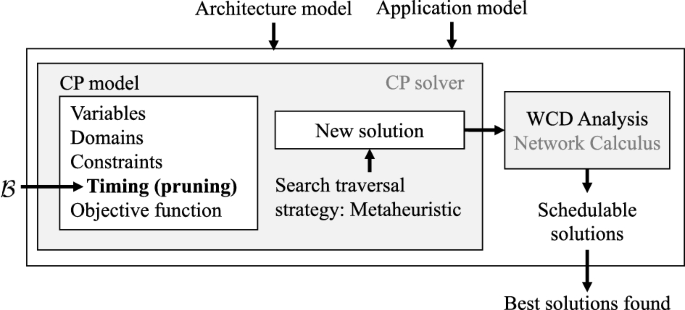

  

  Overview of our CPWO optimization strategy

4.1 Overview

CPWO takes as the inputs the architecture and application models and outputs a set of the best solutions found during search (see Fig. 3). We use CP to search for solutions (the “CP solver” box). CP performs a systematic search to assign the values of variables to satisfy a set of constraints and optimize an objective function, see the “CP model” box: the sets of variables are defined in Sect. 4.3, the constraints in Sect. 4.4 and the objective function in Sect. 4.2. A feasible solution is a valid solution that is schedulable, i.e., the worst-case delays (WCDs) of streams are within their deadlines. Since it is impractical to check for schedulability within a CP formulation, we employ instead the Network Calculus (NC)-based approach from Zhao et al. (2020) to determine the WCDs, see the “WCD Analysis” box in Fig. 3. The WCD Analysis is called every time the CP solver finds a “new solution” which is valid with respect to the CP constraints. The “new solution” is not schedulable if the calculated latency upper bounds are larger than the deadlines of some critical streams.

These timing constraints implement a crude analysis that indicates if a solution may be schedulable and are solely used by the CP solver to eliminate solutions from the search space. These constraints may lead to both “relaxed-pruning” scenarios that are actually unschedulable or “aggressive-pruning” scenarios that eliminate solutions that are schedulable. The proxy function (pruning constraint) can thus be parameterized to trade-off runtime performance for search-space pruning in the CP-model.

The timing constraints assume that for a given stream, its frames in a queue will be delayed by other frames in the same queue, including a backlog of frames of the same stream. A parameter $\mathcal{B}$ is used to adjust the number of frames in the backlog which is an integer number greater than zero, as preemption is not allowed, tuning the pruning level of the CP model’s timing constraints. Note that NC still checks the actual schedulability, so it does not matter if the CP analysis is too relaxed—this will only prune fewer solutions, slowing down the search. However, using overly aggressive pruning runs the risk of eliminating schedulable solutions of good quality. We consider that $\mathcal{B}$ is given by the user, controlling how fast to explore the search space. In the experiments, we adjusted $\mathcal{B}$ based on the feedback from the WCD Analysis and the pruning constraint. If, during a CPWO run, the pruning constraint from Sect. 4.5 was invoked too often, we decreased $\mathcal{B}$, as it was pruning too aggressively; otherwise, if the WCD analysis was invoked too often and was reporting that the solutions were schedulable, we increased $\mathcal{B}$.

We first define the terms needed for the CP model in Table. 2. Then, we continue with the definition of the objective function, model variables, and constraints of the CP model.

Table 2 Definition of terms used in CP model formulation

4.2 CP objective function

The CP solver uses the objective function $\Omega$, which minimizes the average bandwidth usage:

$$\begin{aligned}&\forall p \in P: \Omega = \frac{\sum _{q \in p \cdot Q}\frac{q \cdot w}{q \cdot T}}{\mathcal{N}(P)}. \end{aligned}$$

(1)

Eq. 1 defines the objective function $\Omega$ as the average bandwidth usage in the network. The average bandwidth usage is calculated as the sum of each window’s utilization, i.e., the window length over its period, divided by the total number of windows in the CP model. For each port in each device of the network ($\forall p \in P$), the sum is computed over all windows of the port schedule ($\forall q \in p \cdot Q$). This objective function might be chosen differently depending on the use-case. Other possible formulations could involve minimizing the maximum load on any link or the average end-to-end delay of streams. Note that solutions found by a CP solver are guaranteed to satisfy the constraints defined in Sect. 4.4. In addition, the schedulability is checked with the NC-based WCD Analysis (Zhao et al. 2020).

4.3 Variables

The model variables are the offset, length, and period of each window, see Sect. 2.2. For each variable, we define a domain which is a set of finite values that can be assigned to the variable. CP decides the values of the variables as an integer from their domain in each visited solution during the search. The domains of offset $q \cdot \phi$, length q.w, and period q.T variables are defined, respectively, by

$$\begin{aligned} \begin{aligned}&\forall p \in P,\forall q \in p \cdot Q:\\&0 < q \cdot T \le \frac{\mathcal{K}(p)}{[v_a, v_b].mt},\quad 0 \le q \cdot \phi \le \frac{\mathcal{K}(p)}{[v_a, v_b].mt},\\&\frac{\mathcal{L}(q)}{[v_a, v_b].mt \times [v_a, v_b].C} + \mathcal{G}\mathcal{B}(q) \le q \cdot w \le \frac{\mathcal{K}(p)}{[v_a, v_b].mt}. \end{aligned} \end{aligned}$$

(2)

The domain of the window period is defined in the range from 0 to the hyperperiod of the respective port p, i.e., the Least Common Multiple (LCM) of all the stream periods forwarded via the port. The window period is an integer and cannot be zero. The domain of the window offset is defined in the range from 0 to the hyperperiod of the respective port p. Finally, the domain of the window length is defined in the range from the minimum accepted window length to the hyperperiod of the respective port p. The minimum accepted window length is the length required to transfer the largest frame from all streams assigned to the queue q, protected by the guard band $\mathcal{G}\mathcal{B}(q)$ of the queue. A port p is attached to only one link $[v_a, v_b]$; and values and domains are scaled by the macrotick mt of the respective link.

4.4 Constraints

The first three constraints need to be satisfied by a valid solution: (1) the window is valid, (2) two windows in the same port do not overlap, and (3) the window bandwidth is not exceeded. The next two constraints reduce the search space by restricting the periods of (4) queues and (5) windows to harmonic values in relation to the hyperperiod. Harmonicity may eliminate some feasible solutions but we use this heuristic strategy to speed up the search. Finally, we introduce a constraint that limits the size of the resulting GCL configuration to be smaller than or equal to a given maximum (Eq. (8)). This is necessary since some resource-constrained TSN devices may only allow a limited GCL size per port.

• (1) The window validity constraint (Eq. (3)) states that the offset plus the length of a window should be smaller or equal to the window’s period:

  $$\begin{aligned} \begin{aligned}&\forall p \in P,\forall q \in p \cdot Q: \quad (q \cdot w + q \cdot \phi ) \le q \cdot T. \end{aligned} \end{aligned}$$

  (3)

• (2) Non-overlapping constraint (Eq. (4)). Since we search for solutions in which windows of the same port do not overlap, the opening or closing of each window on the same port (defined by its offset and the sum of its offset and length, respectively) is not in the range of another window, over all period instances:

  $$\begin{aligned}&\forall p \in P,\forall q \in p \cdot Q, \forall q^{\prime} \in p \cdot Q, T_{q,q^{\prime}}= max(q \cdot T, q^{\prime}T), \\&\forall a \in [0,T_{q,q^{\prime}}/q \cdot T),\forall b \in [0,T_{q,q^{\prime}}/q^{\prime} \cdot T): \\&(q \cdot \phi + q \cdot w+ a \times q \cdot T) \le (q^{\prime} \cdot \phi + b \times q^{\prime} \cdot T) \vee \\&(q^{\prime} \cdot \phi + q^{\prime} \cdot w + b \times q^{\prime} \cdot T) \le (q \cdot \phi + a \times q \cdot T) \end{aligned}$$

  (4)

• (3) The bandwidth constraint (Eq. (5)) ensures that all the windows have enough bandwidth for the assigned streams:

  $$\begin{aligned} \begin{aligned}&\forall p \in P,\forall q \in p \cdot Q: \frac{q \cdot w}{q \cdot T}\ge \sum _{f \in \mathcal{F}(q)} \frac{f \cdot l}{f \cdot T}. \end{aligned} \end{aligned}$$

  (5)

  where $\mathcal{F}(q)$ is the set of streams assigned to the queue q.

• (4) The port period constraint (Eq. (6)) imposes that the periods of all the queues in a port should be harmonic. This constraint is used to avoid window overlapping and to reduce the search space. We note that this constraint has no influence on the period design of the streams in the system. The period of the given streams and the period of the windows that our solutions determine are two different entities that affect each other but are not restricted by one another. A stream may have any period, and we only constrain the period the resulting GCL windows in the schedule. It is necessary to constrain the GCL window period since it is an optimization variable, and if left unconstrained, there would be infinite possible solutions.

  $$\begin{aligned} \begin{aligned}&\forall p \in P,\forall q \in p \cdot Q, \forall q^{\prime} \in p \cdot Q: (q.T\%q^{\prime} \cdot T=0) \vee (q^{\prime} \cdot T\%q.T=0). \end{aligned} \end{aligned}$$

  (6)

• (5) The period limit constraint (Eq. (7)) reduces the search space by considering window periods q.T that are harmonic with the hyperperiod of the port $\mathcal{K}(p)$ (divide it):

  $$\begin{aligned} \begin{aligned}&\forall p \in P,\forall q \in p \cdot Q: \quad \mathcal{K}(p)\%{q.T}= 0. \end{aligned} \end{aligned}$$

  (7)

• (6) The GCL size constraint (Eq. (8)) mandates that the number of open/close entries in the resulting GCL is below a given maximum defined by $GCL_{max}$. Since in the previous constraint we imposed that any window period q.T is harmonic with the hyperperiod of the port $\mathcal{K}(p),$ we need to make sure that the resulting number of open/close windows until the hyperperiod of the port is smaller than or equal to the given maximum. Since we do not know if windows on different queues are back-to-back, the state transition from the closing event of one window may not coincide with the opening event of another window. Hence, each window can potentially introduce two entries in the GCL table, one for opening the window and another for closing it. Therefore the maximum number of GCL entries can be bounded as follows:

  $$\begin{aligned} \begin{aligned}&\forall p \in P: \quad \sum _{q \in p \cdot Q} 2\times \bigg \lceil \frac{\mathcal{K}(p)}{{q.T}}\bigg \rceil \le GCL_{max}. \end{aligned} \end{aligned}$$

  (8)

4.5 Timing constraints

As mentioned, it is infeasible to use a Network Calculus-based worst-case delay analysis to check the schedulability of each solution visited. Thus, we have defined a Timing Constraint as a way to prune the search space. Every solution that is not eliminated via this timing constraint is evaluated for schedulability with the NC WCD analysis. The timing constraint is a heuristic that prunes the search space of (potentially unschedulable) solutions; it is not a sufficient nor a necessary schedulability test. The timing constraint is related to the optimality of the solution, not to its correctness in terms of schedulability. An overly aggressive pruning may eliminate good quality solutions, and too little pruning will slow down the search because the NC WCD analysis is invoked too often.

The challenge is that the min+ algebra used by NC cannot be directly expressed in the first-order formulation of CP. However, the NC formulation from Zhao et al. (2020) has inspired us to define the CP timing constraints. The Timing Constraint is defined in Eq. (9) and uses the concepts of window capacity $\mathcal{W}_C$ and transmission demand $\mathcal{W}_D$ to direct the CP solver to visit only those solutions where the capacity of each window, i.e., the amount of time available to transmit frames assigned to its queue, is greater than or equal to its transmission demand, i.e., the amount of transmission time required by the frames in the queue. A window capacity larger than the transmission demand indicates that a solution has a high chance to be schedulable:

$$\begin{aligned} \begin{aligned}&\forall p \in P,\forall q \in p \cdot Q: \mathcal{W}_D \le \mathcal{W}_C. \end{aligned} \end{aligned}$$

(9)

Thus, we first calculate the capacity $\mathcal{W}_C$ of each window within the hyperperiod. This capacity is similar to the NC concept of a service curve, and its calculation is similar to the service curves proposed in the literature (Wandeler 2006) for resources that use Time-Division Multiple Access (TDMA), which is how our windows behave. For e.g., a window with a period of 10 μs, a length of 4 μs, and an offset of 3 μs; forwards 150 bytes over a 100 Mbps link in a hyperperiod of 30 μs. In Fig. 4, the capacity of such a window is depicted where the blue line shows the throughput of the window for transferring data. The capacity increases when the window opens (the rising slopes of the curve). The effect of window offset on the capacity (the area under the curve) can be observed in the figure. The function $\mathcal{W}_C$ calculates the area under the curve to characterize the amount of capacity for a window in a hyperperiod, defined in Eq. (10), where the link $[v_a, v_b]$ is attached to the port p and assigned to the queue q; and function $\mathcal{Y}$ captures the transmission time of a single byte through link $[v_a, v_b]$.

To calculate the area under the curve, we consider 3 terms that are $S_1$, $S_2$, and $S_3$. They represent the total area under the curve caused by the window length, the window closure in the remainder of the window period, and the window period, respectively. The value for $S_1$ equals to the area of three triangles, each with the base of 4 μs and the height of 50 Bytes. Similarly, the value for $S_2$ equals to the three rectangles, each with a length of 3 μs and a width of 50 Bytes. Lastly, the value for $S_3$ equals to the area of three triangles with a base of 10 μs and a height of 50 Bytes. The $\mathcal{W}_C$ value of the example in Fig. 4 is 2250 Bytes × μs, where the S terms are shown.

$$\begin{aligned} \begin{aligned}&\forall p \in P,\forall q \in p \cdot Q:\\&I = \frac{\mathcal{K}(p)}{q.T}, \quad J=\frac{(q.w - \mathcal{G}\mathcal{B}(q))\times \mathcal{Y}([v_a, v_b])}{[v_a, v_b].C},\\&S_1 = I \times \frac{q.w \times J}{2}, \quad S_2= I \times (q.T - q.w. - q.\phi ) \times J,\\&S_3=\frac{I\times (I-1)}{2} \times q.T \times J, \quad \mathcal{W}_C=S_1 + S_2+S_3 \end{aligned} \end{aligned}$$

(10)

Secondly, we calculate the transmission demand $\mathcal{W}_D$ using Eq. (11), where $\mathcal{R}(q)$ captures all the streams that are assigned to the queue q. The transmission demand is inspired by the arrival curves of NC. These are carefully determined in NC considering that the streams pass via switches and may change their arrival patterns (Zhao et al. 2020). In our case, we have made the following simplifying assumptions to be able to express the “transmission demand” in CP. We assume that all streams are strictly periodic and arrive at the beginning of their respective periods. This is “optimistic” with respect to NC in the sense that NC may determine that some of the streams have a bursty behavior when they reach our window. To compensate for this, we consider that those streams that arrive from a switch may be bursty and thus have a backlog $\mathcal{B}$ of frames that have accumulated; streams that arrive from ESs do not accumulate a backlog. It is also noteworthy that the value of $\mathcal{B}$ being an integer or decimal depends on whether preemption (IEEE 802.1Qbu) is supported/enabled for the critical flows in the network, i.e., if critical flows are marked as express, and the devices support preemption. When frames can be preempted, the value of $\mathcal{B}$ can be chosen from $\mathbb {R}^+$, which implies that also fragments of frames are allowed to be backlogged. If preemption is not supported or enabled for the critical frames, the value of $\mathcal{B}$ can only take integer values greater than or equal to 1, specifying how many full frames can be backlogged. In this work, we consider that critical flows are not preemptable; hence, we consider only integers greater than zero for $\mathcal{B}$. Figure 5 shows three streams, $f_1$ to $f_3$, and only $f_3$ arrives from a switch and hence will have a backlog of frames captured by the stream denoted with $f^{\prime}_3$ (we consider a $\mathcal{B}$ of 1 in the example). We also assume that the backlog $f^{\prime}_3$ will not arrive at the same time as the original stream $f_3$, and instead, it is delayed by a period. Again, this is a heuristic used for pruning, and the actual schedulability check is done with the NC analysis. So, the definition of the “transmission demand” does not impact correctness, but, as discussed, it will impact our algorithm’s ability to search for solutions.

Since, in our case, the deadlines can be larger than the periods, we also need to consider, for each stream, bursts of frames coming from SWs and an additional frame for each stream coming from ESs (the ES periods are not synchronized with the SWs GCLs). Since we do not perform a worst-case analysis, we instead use a backlog parameter $\mathcal{B}$, capturing the possible number of delayed frames in a burst within a stream forwarded from another SW. Note that as explained in the overview at the beginning of Sect. 4, $\mathcal{B}$ is a user-defined parameter that controls the “pruning level” of our timing constraint, i.e., how aggressively it eliminates candidates from the search space depending on the preemption.

Fig. 4

Example capacity for a window

We give an example in Fig. 5 where the streams $f_1\langle <50,5,0,5\rangle$ and $f_2\langle 60,6,0,6\rangle$ have been received from an ES and the stream $f_3\langle 100,15,0,15\rangle$ has been received from a SW. For the stream $f_3$ forwarded from a previous switch, we consider that one instance of the stream (determined by the backlog parameter $\mathcal{B} = 1$), let us call it $f^{\prime}_3$, may have been delayed and received together with the current instance $f_3$. This would cause a delay in the reception of the streams in the current node. The reception curve in Fig. 5 is the sum of curves for each stream separately in a hyperperiod of 30 μs.

Fig. 5

Example capacity and transmission demand for a window

We give the general definition of the transmission demand value $\mathcal{W}_D$ as the area under the curve for the accumulated data amount of received streams and backlogs of the streams arrived from switches in a hyperperiod. For calculating the transmission demand $\mathcal{W}_D$, we consider 2 terms that are $A_1$ and $A_2$ for each stream. The term $A_1$ calculates the area under the curve for the accumulated data of all streams assigned to the queue q captured by $\mathcal{R}(q)$, in a hyperperiod. Any frames of all streams $\mathcal{R}(q)$ have arrived at the beginning of their period. Considering the hyperperiod of the received streams which is denoted by $\mathcal{K}(p)$, each stream will have I instances in this queue. For each instance i, the area under the curve consists of i rectangles with the length of the stream period and the width of the stream size. Thus for all I instances of the stream the area under the curve is equal to $\frac{I\times (I+1)}{2}$ rectangles.

The term $A_2$ calculates the area under the curve for the accumulated backlog data of the streams arrived from a switch captured by $\mathcal{X}(q)$. The backlog data of the streams $\mathcal{X}(q)$ are delayed for a period and controlled by $\mathcal{B}$, which captures the number of backlogs. Similarly, the area under the curve for the stream backlogs consists of the number of rectangles with the length of the stream period and the width of the stream size. The only difference is that the stream has $\mathcal{B}$ instances less. Thus, the number of rectangles equals to $\frac{I\times (I+1-2\times \mathcal{B})}{2}$. The function $\mathcal{W}_D$ returns 16,650 $Bytes\times \mu s$ in our example, see also Fig. 5 for the values of the terms $A_1$ and $A_2$.

$$\begin{aligned} \begin{aligned}&\forall p \in P,\forall q \in p \cdot Q, \forall f \in \mathcal{R}(q), \forall f^{\prime} \in \mathcal{X}(q):\\&I = \frac{\mathcal{K}(p)}{f \cdot T}, \quad I^{\prime} = \frac{\mathcal{K}(p)}{f^{\prime} \cdot T}\\&A_1=\frac{I \times (I+1)}{2} \times f \cdot T \times f \cdot l,\\&A_2=\frac{I^{\prime} \times (I^{\prime}+1 - 2\times \mathcal{B})}{2} \times f^{\prime} \cdot T \times f^{\prime} \cdot l,\\&\mathcal{W}_D= A_1 + A_2 \end{aligned} \end{aligned}$$

(11)

Please note that the correctness of the constraints (Eq. (3), (4), (5)) follows from the implicit hardware constraints of 802.1Q(bv) (see the discussion in Craciunas et al. 2016; Serna Oliver et al. 2018) while other constraints (Eq. (6), (7)) are used to limit the placement of GCL windows and are not related to correctness, just to optimality. Since the transmission of frames is decoupled from the GCL windows, the schedule’s correctness concerning the end-to-end latency of streams is always guaranteed due to the NC analysis, which is intertwined in the schedule step.

5 Simulated Annealing Window Optimization (SAWO)

The previously described CPWO delivers good results in a reasonable time for small problem sizes. However, for larger problem sizes, the method either becomes intractable, or the search space pruning has to be done very aggressively, leading to a degradation in the quality of the results. For such intractable problems, optimal algorithms such as Branch and Bound and Integer Linear Programming require an exponentially increasing time with increasing input size. Therefore we propose a metaheuristic algorithm that is aimed to be scalable for large problem sizes while still offering good quality solutions. Metaheuristics are designed to find good quality solutions while still being scalable for large problem sizes but are not guaranteed to find an optimal (or any) solution (Burke and Kendall 2014). A plethora of metaheuristic approaches have been proposed in the literature for intractable problems (Burke and Kendall 2014; Campelo and Aranha 2022). In this paper, we have developed a SA-based metaheuristic solution.

Our SAWO algorithm is shown in Algorithm 1. The key feature of SA is that it avoids getting stuck in a local optimum by accepting worse intermediate solutions with a certain probability, which decreases throughout the search (Kirkpatrick et al. 1983; Burke and Kendall 2014). The likelihood of considering a worse solution (compared to the current solution) depends on the worsening of the objective function and a temperature parameter t (Voß and Woodruff 2002). In SA, the temperature starts from an initial temperature $T_{start}$ (line 3) and is decreased in every iteration with a factor $0< \alpha < 1$ (line 16).

SA starts from an initial solution $\Phi$ (line 1, see Sect. 5.1) which is evaluated using the objective function $\Omega^{SA}$ (line 2), see Sect. 5.2 for details. When there are no infeasible streams the objective functions for CPWO and SAWO are identical and thus comparable. If there are infeasible streams, we penalize this in the SAWO solution in order to guide the search (see Sect. 5.2).

SA iterates until a stopping criterion, like a timeout or iteration limit, is satisfied (lines 4–17). In every iteration, we generate a random “neighbor” of the current solution (line 5) and calculate the difference $\delta$ between its objective value $\Omega^{SA}_{new}$ and the objective value $\Omega^{SA}$ of the current solution (line 7). Section 5.3 presents how we generate a neighbor solution. If the new objective value is smaller, we accept the new solution as the current (and possibly best, see lines 11–14). However, we also sometimes accept a worse neighbor solution. This is the case if a random value (between 0 and 1) is smaller than an “acceptance probability function” $e^{\frac{\delta }{t}}$ (see line 8). This acceptance probability function decreases with a larger $\delta$, i.e., we are less likely to accept worse neighbors if they are further from the current solution, or a smaller temperature, i.e., the probability of accepting worse neighbors decreases during the search. We use a time limit as the stopping criterion.

Algorithm 1

Simulated Annealing Window Optimization (SAWO)

5.1 Initial solution

The goal of the InitialSolution function, shown in Algorithm 2, is to find a good starting point for SA. We start out by choosing a common period for all windows in the port, which helps speed up overlap and worst-case latency calculations. This also means that there is a maximum of two GCL entries per queue, which means that a $GCL_{max} \ge 16$ will suffice for this solution. The choice of this period is important: A larger period means longer worst-case latencies but less bandwidth occupation since the distance between two consecutive windows is longer (in the worst-case a stream arrives right at the moment when it can’t fit into the current window anymore, requiring it to wait a full window period). We choose the minimum period that is larger than the combined length of all streams in the port from a set containing all stream periods, their greatest common divisor (GCD), and half of that value (lines 2–5). We found empirically that choosing a period from this set of values provides a good balance between minimizing worst-case delays and bandwidth occupation. The half GCD value is often useful for cases in which we have a large GCD of the given stream periods but tight deadlines (e.g. equal to the stream period). In the worst-case a stream gets delayed by approximately one window period per hop, so having those small window periods becomes very important. For topologies with very long routes, it could be worthwhile to consider even smaller fractions of the GCD in the set. Then we decide the length for each window (line 10). It has to be at least as long as the total sending time of all streams in that queue (line 8), and its size relative to the period of the window has to be at least as big as the stream sizes relative to their period (line 9). Finally, we align the windows in the different queues so they do not overlap (lines 11–12), since, in the worst-case, an overlapping part of a window has to be considered occupied.

Algorithm 2

SA initial solution

5.2 SA objective function

The objective function $\Omega^{SA}$ used inside SA is shown in Eq. (12). The difference between $\Omega^{SA}$ and $\Omega$ used by CP (Eq. (1), Sect. 4.2) is that $\Omega$ minimizes the average bandwidth usage and then uses timing constraints and network calculus to check that a solution is schedulable.

$\Omega^{SA}$ has two components: The first component $\Omega^{bw}$ is measuring the bandwidth consumed by all windows across all ports on average, and is equivalent $\Omega$. The second component $\Omega^{inf}$ is the number of streams that miss their deadline, also called infeasible streams. Thus, instead of using the schedulability as a constraint as in the CP formulation, we allow SA to visit unschedulable solutions in the hope of driving the search towards schedulable solutions. The amount of infeasible streams is determined by running the NC-based worst-case delay analysis of Zhao et al. (2020) with the given set of windows. Since the average consumed bandwidth is at most 1 (equals to 100%), any missed deadlines will increase the objective value and thus drive the search to schedulable solutions that decrease $\Omega^{inf}$, which dominates the objective function when a solution is not schedulable. The weights $w_a$ and $w_b$ in Eq. (12) can be used to control the relative importance of the two components, e.g., when a system engineer prefers lower bandwidth at the expense of schedulability, $w_a$ can be increased and $w_b$ decreased. In our experiments, we have used $w_a = w_b = 1$, which we found is a good choice when searching for schedulable solutions.

$$\begin{aligned}&\Omega^{SA} = w_a \times \Omega^{bw} + w_b \times \Omega^{inf}, \text { where} \end{aligned}$$

(12)

$$\begin{aligned}&\Omega^{bw} = \frac{\sum _{q \in p \cdot Q} \frac{q.w}{q.T}}{\mathcal{N}(P)}, \forall p \in P \\&\Omega^{inf} = |\{f \mid f \in \mathcal{F} \wedge m_i^{dest(f)}.\phi + m_i^{dest(f)}.L - m_i^{src(f)}.\phi > f \cdot D - \delta \}|\end{aligned}$$

(13)

5.3 Neighbor function

The purpose of the $\text {RandomNeighbor}(\Phi ,p_{mv})$ function in Algorithm 1 is to select a close neighbor of the current solution $\Phi$. A neighbor is generated by performing a transformation (also called “moves”) on the current solution. This transformation function is designed such that the SA search will have good coverage of the solution space. The solution space, in our case, includes all solutions that have one window per queue, with a minimum length and without overlap of windows in the same port. Our neighbor function uses two different moves to change the current solution:

• MoveWindow: Selects a random occupied queue. Changes the window offset to a random value within the range of all offsets where the window will not overlap with windows in other queues on the same port. This move occurs with a given probability of $p_{mv}$.

• ChangeWindowSize: Selects a random occupied queue. Changes the window size to a random value in the range between the minimum window size and the maximum size before an overlap with another window in the same port would occur. This move is applied with a probability of $1-p_{mv}$.

We have used a value of $p_{mv} = 0.8$ in the experiments. This makes it more likely for a MoveWindow move to occur, which is usually more impactful, since the window sizes are already set to reasonable initial values by the initial solution, while the window alignment across ports is not very good yet.

6 Related work

Scheduling homogeneous TSN networks in which all devices are scheduled and synchronized has been solved in various forms using heuristics (Nayak et al. 2018; Mahfouzi et al. 2018; Pahlevan and Obermaisser 2018; Pahlevan et al. 2019; Vlk et al. 2022; Berisa et al. 2022) and optimal ILP- or SMT-based approaches (Craciunas et al. 2016; Serna Oliver et al. 2018; Falk et al. 2018; Vlk et al. 2021; Zhou et al. 2021a, b). The most relevant results for providing real-time communication properties in TSN networks, to which we compare our approach, have been presented in Craciunas et al. (2016), Serna Oliver et al. (2018), Pop et al. (2016), Dürr and Nayak (2016) (summarized in Table 3). Originally, the TSN scheduling problem was addressed in Craciunas et al. (2016) for fully deterministic ST traffic temporal behavior and temporal isolation between ST and non-ST (e.g., AVB, BE) streams/flows, similar to TTEthernet (Steiner 2010; Craciunas and Serna Oliver 2016). In our comparison, we call this method 0GCL, since, besides enforcing the required end-to-end latency of ST streams, the scheduling constraints also impose a strictly periodic frame transmission resulting in 0 jitter forwarding of critical traffic. The work in Pop et al. (2016) uses heuristics instead of SMT-solvers to solve the 0-jitter scheduling problem in order to improve scalability while also minimizing the end-to-end latency of AVB streams. In Serna Oliver et al. (2018), which we call Frame-to-Window-based, the 0-jitter constraint of Craciunas et al. (2016) is relaxed by allowing more variance in the transmission times of frames over the hops of their routed paths. This increases the solution space at the expense of increased complexity in the correctness constraints. The method in Serna Oliver et al. (2018) can be viewed as window-based scheduling, but, unlike our approach, it requires a unique mapping between GCL windows and frames in order to avoid non-determinism in the queues. In Dürr and Nayak (2016) the TSN scheduling problem is reduced to having one single queue for ST traffic and solving it using Tabu Search that optimizes the number of guard-bands in order to optimize bandwidth usage.

The main goal of the aforementioned works is similar to ours, namely to allow temporal isolation and compositional system design for ST streams with end-to-end guarantees and deterministic communication behavior. However, all previous methods impose that the end-systems from which the ST traffic originates are synchronized to the rest of the network and have the IEEE 802.1Qbv timed-gate mechanism (i.e., they are scheduled). The open gate windows are then either a result of the frame transmission schedule (Craciunas et al. 2016; Pop et al. 2016) or are uniquely associated with predefined subsets of frames (Serna Oliver et al. 2018). However, the above property is a significant limitation. In many use cases, especially in the industrial and automotive domains (cf. Schriegel et al. 2018), the end-systems are usually off-the-shelf sensors, microcontrollers, industrial PCs, and edge devices that do not have TSN capabilities.

The work in Reusch et al. (2020) proposed a more naive window-based approach (WND) in which the GCL window offsets on different network nodes are not included, thereby essentially limiting the mechanisms by requiring all GCL windows to be lined up between bridges. Moreover, Reusch et al. (2020) uses a less advanced analysis step (cf. Zhao et al. 2018) in the scheduling decisions and a more naive heuristic approach. These limiting assumptions were relaxed in Barzegaran et al. (2022), which has proposed a Constraint Programming solution to the window optimization problem.

The work in Hellmanns et al. (2020b) proposes a scheduling model for TSN networks in industrial automation with different traffic types and a hierarchical scheduling procedure for isochronous traffic. The method proposed in Hellmanns et al. (2020a) adopts a so-called stream batching approach, which can be classified as window-based in that it can assign multiple frames to the same GCL window. However, the end-points still need to be synchronized and scheduled, and, additionally, the worst-case delay bounds within the batch windows may lead to deadline misses since they are not based on formal methods like the network calculus framework in our approach. In Shalghum et al. (2021), the authors present an NC-based analysis for overlapping GCL windows with less pessimistic latency bounds and a scheduling algorithm (FWOS) that focuses on maximizing the allowable overlap of GCL windows to increase the bandwidth of unscheduled traffic without jeopardizing the schedulability of ST traffic. As opposed to our method, Shalghum et al. (2021) cannot guarantee the schedulability of traffic arriving from unscheduled or unsynchronized end-systems.

Classical approaches like strict priority (SP) and AVB (Institute of Electrical and Electronics Engineers 2011) do not require a time-gate mechanism and also work with unscheduled end-systems. In order to provide response-time guarantees, a worst-case end-to-end timing analysis through methods like network calculus (Schmitt et al. 2003; De Azua and Boyer 2014) or Compositional Performance Analysis (CPA) (Diemer et al. 2012) are used. In Zhao et al. (2017), Zhao et al. (2014), Boyer et al. (2016), the rate-constrained (RC) streams of TTEthernet (Issuing Committee 2011; Steiner et al. 2011) are analyzed using network calculus. Other works, such as Wandeler and Thiele (2006a), Khanh and Mifdaoui (2014), study the response-time analysis for TDMA-based networks under the strict priority (SP) and weighted round-robin (WRR) queuing policies. Zhao et al. (2020) present a worst-case delay analysis, which we use in this paper, for determining the interference delay between ST traffic on the level of flexible GCL windows. Using SP only or leaving all ST windows open for the entire hyperperiod duration (which amounts to SP for ST traffic) will not result in the same response-time bounds and schedulability as our method. Our method can delay specific high-priority ST streams when needed to allow a timely transmission of lower-priority ST streams with a much tighter deadline. Unlike SP, our method uses the IEEE 802.1Qbv timed gates to open and close queues as needed to enforce isolation between traffic classes. With pure SP (or when leaving all gates open at all times), misbehaving end-systems (e.g., babbling-idiot failures) will disrupt all (lower-priority) traffic classes, potentially leading to a loss of all real-time properties of the network.

In Vlk et al. (2020), the authors present hardware enhancements to standard IEEE 802.1Qbv bridges (along with correctness constraints for the schedule generation) that remove the need for the isolation constraints between frames scheduled in the same egress queue defined in Craciunas et al. (2016). Another hardware adaptation for TSN bridges, which has been proposed by Heilmann and Fohler (2019) is to increase the number of non-critical queues in order to improve the bandwidth utilization without impacting the guarantees for critical messages.

Lastly, we look at our CP optimization strategy to improve scalability and performance. In our CPWO method, we combine an exact CP solver with a metaheuristic search within a loop to improve scalability. A similar direction and aim, but using a very different method, is given in Luteberget et al. (2021), where the authors combine an SMT-based method with a discrete event simulation within a counterexample-guided abstraction refinement loop and apply it to railway design.

6.1 In-depth formal comparison

In this section, we compare FWND with the related work in terms of the objectives and constraints. The related work on ST scheduling using 802.1Qbv consists of: (i) zero-jitter GCL (0GCL) (Craciunas et al. 2016; Pop et al. 2016), (ii) Frame-to-Window-based GCL (FGCL) (Serna Oliver et al. 2018), and (iii) Window-based GCL (WND) (Reusch et al. 2020).

Table 3 Scheduling approaches in TSN

We summarize the requirements of the ST scheduling approaches from the related work and our FWND approach in the first column of Table 3. The first three requirements refer to the device capabilities needed for the different approaches, and the next seven rows summarize which constraints and isolation requirements are needed by which approach. The last two rows present the requirements of the complexity of the optimization problem that needs to be solved to provide a solution for the respective approach.

To better understand the fundamental differences and the similarities (in terms of the imposed correctness constraints and schedulability parameters) between our work and the approaches that require synchronized and scheduled end systems, we briefly reiterate the formal constraints of previous work. We describe, based on (Craciunas et al. 2016; Craciunas and Serna Oliver 2017; Serna Oliver et al. 2018), the relevant scheduling constraints for creating correct TSN schedules when using frame- and window-based methods. Table 3 shows which of these are needed by which approach.

We adapt some notations from Craciunas et al. (2016), Craciunas and Serna Oliver (2017) to describe the constraints and assume certain simplifications without loss of generality, e.g. the macrotick is the same in all devices, all streams have only one frame per period, the propagation delay $d_p$ is 0. We refer the reader to Craciunas et al. (2016), Serna Oliver et al. (2018) for a complete and generalized formal definition of the correctness constraints. We denote the messages (frames) of a stream $f_i$ on a link $[v_a, v_b]$ as $m_i^{[v_a, v_b]}$. A message $m_i^{[v_a, v_b]}$ is defined by the tuple $\langle m_i^{[v_a, v_b]}.\phi , m_i^{[v_a, v_b]}.l \rangle ,$ denoting the transmission time and duration of the frame on the respective link (Craciunas et al. 2016; Craciunas and Serna Oliver 2017).

6.2 Frame constraint

Any frame belonging to a critical stream has to be transmitted between time 0 and its period $T_i$. To enforce this, we have the frame constraint from Craciunas et al. (2016):

$$\begin{aligned}&\forall f_i \in \mathcal{F}, \forall [v_a, v_b] \in f_i \cdot r : \\&\quad \left( m_i^{[v_a, v_b]}.\phi \ge 0\right) \wedge \left( m_i^{[v_a, v_b]}.\phi \le f_i \cdot T - m_i^{[v_a, v_b]}.l \right) . \end{aligned}$$

6.3 Link constraint

A physical constraint of Ethernet-based networks is that only one frame can be on the wire from one port to another at a time. In Craciunas et al. (2016) and Serna Oliver et al. (2018) this constraint is expressed as windows on two different queues of the same egress port not being able to overlap. In Reusch et al. (2020) and the FWND method presented in this paper, windows on different queues may overlap, leading to added interference delays since naturally, only one frame can be sent on the physical link at a time. Still, in both Reusch et al. (2020) and the FWND, solutions where windows overlap are excluded since there is no added improvement from such schedules.

The link constraint adapted from Craciunas et al. (2016) is hence:

$$\begin{aligned}&\forall [v_a, v_b] \in \varvec{E}, \forall m_i^{[v_a, v_b]}, m_j^{[v_a, v_b]} (i \ne j), \\&\forall a \in [0, hp_{i}^{j}/f_i \cdot T - 1 ], \forall b \in [0, hp_i^j/f_j.T - 1]:\\&\Bigl (m_i^{[v_a, v_b]}.\phi + a\times f_i \cdot T \ge m_j^{[v_a, v_b]}.\phi + b\times f_j.T + m_j^{[v_a, v_b]}.l \Bigr )\vee \\&\Bigl (m_j^{[v_a, v_b]}.\phi + b\times f_j.T \ge m_i^{[v_a, v_b]}.\phi + a\times f_i \cdot T + m_i^{[v_a, v_b]}.l\Bigr ), \end{aligned}$$

where $hp_i^j = lcm(f_i \cdot T, f_j.T)$ is the hyperperiod of $f_i$ and $f_j.$

6.4 Bandwidth constraint

The bandwidth constraint expressed explicitly in our method ensures that there is no infinite backlog, i.e., the windows for the streams are large enough that the frames of the streams can be transmitted at some point. In 0GL (Craciunas et al. 2016) this constraint is implicit since the schedule is created without the separation of streams and windows, meaning that each window is large enough to transmit the respective frames. In Serna Oliver et al. (2018) there is no one-to-one assignment between frames and windows; however, the window size constraint is equivalent to the bandwidth constraint. Using this constraint the length of the gate open window is required to be equal to the sum of the frame lengths that have been assigned to it. In Reusch et al. (2020) the bandwidth constraint is explicit in the conditions for the correctness of the schedule generation.

6.5 Stream transmission constraint

The stream transmission constraint expresses that the propagation of frames of a stream follows the sequential order along the path of the stream. This (optional) constraint enforces that a frame is forwarded by a device only after it has been received at that device also taking into account the network precision, denoted with $\delta$:

$$\begin{aligned}&\forall f_i \in \mathcal{F}, \forall [v_a, v_x], [v_x, v_b] \in f_i \cdot r, \forall m_i^{[v_a, v_x]}, \forall m_i^{[v_x, v_b]}: \\&m_i^{[v_x, v_b]}.\phi - \delta \ge m_i^{[v_a, v_x]}.\phi + m_i^{[v_a, v_x]}.l. \end{aligned}$$

In FWND (and also in Reusch et al. 2020) this constraint is not explicitly needed since there is no predefined assignment of frames to windows and hence, there is no explicit ordering needed in sequential hops along the route of a stream, i.e., the transmission GCL window which is used at a certain time will depend on the enqueueing order at that time in the egress queue.

6.6 End-to-end constraint

The maximum end-to-end latency constraint (expressed by the deadline $f_i \cdot D$) enforces a maximum time between the sending and the reception of a stream. We denote the sending link of stream $f_i$ with $src(f_i)$ and the last link before the receiving node with $dest(f_i)$. The maximum end-to-end latency constraint (Craciunas et al. 2016) is hence

$$\begin{aligned}&\forall f_i \in \mathcal{F}: m_i^{dest(f_i)}.\phi + m_i^{dest(f_i)}.L - m_i^{src(f_i)}.\phi \le f_i \cdot D - \delta . \end{aligned}$$

Here again, the network precision $\delta$ needs to be taken into account since the local times of the sending and receiving devices can deviate by at most $\delta.$

6.7 802.1Qbv stream/frame isolation

Due to the non-determinism problem in TSN (cf. Sect. 2.2), previous solutions (e.g., Craciunas et al. 2016; Serna Oliver et al. 2018) need an isolation constraint that maintains queue determinism. We refer the reader to Craciunas et al. (2016) for an in-depth explanation and only summarize here the stream and frame isolation constraint adapted from Craciunas et al. (2016). Let $m_i^{[v_a, v_b]}$ and $m_j^{[v_a, v_b]}$ be, respectively, the frame instances of $f_i \in \mathcal{F}$ and $f_j \in \mathcal{F}$ scheduled on the outgoing link $[v_a, v_b]$ of device $v_a$. Stream $f_i$ arrives at the device $v_a$ from some device $v_x$ on link $[v_x, v_a]$. Similarly, stream $f_j$ arrives from another device $v_y$ on incoming link $[v_y, v_a]$. The simplified stream isolation constraint adapted from Craciunas et al. (2016), under the assumption that the macrotick of the involved devices is the same, is as follows:

$$\begin{aligned}&\forall [v_a, v_b] \in \varvec{E}, \forall m_i^{[v_a, v_b]}, m_j^{[v_a, v_b]} (i\ne j), \\&\forall a \in [0, hp_{i}^{j}/f_i \cdot T - 1 ], \forall b \in [0, hp_i^j/f_j.T - 1]:\\&\Bigl (m_i^{[v_a, v_b]}.\phi + a\times f_i \cdot T + \delta \le m_j^{[v_y, v_a]}.\phi + b\times f_j.T \Bigr ) \vee \\&\Bigl (m_j^{[v_a, v_b]}.\phi + b\times f_j.T + \delta \le m_i^{[v_x, v_a]}.\phi + a\times f_i \cdot T \Bigr ). \end{aligned}$$

Here again $hp_i^j = lcm(f_i \cdot T, f_j.T)$ is the hyperperiod of $f_i$ and $f_j$. The constraint ensures that once a stream arrives at a device, no other stream can enter the device until the first stream has been sent.

The above constraints apply to frames that are placed in the same queue on the egress port. However, the scheduler may choose (if possible) to place streams in different queues, isolating them in the space domain. Hence, the complete constraint (Craciunas et al. 2016) for frame/stream isolation for two streams $f_i$ and $f_j$ scheduled on the same link $[v_a, v_b]$ can be expressed as

$$\begin{aligned}&\Bigl ( \Phi _{[v_a, v_b]}(f_i, f_j) \Bigr ) \vee \Bigl (m_i^{[v_a, v_b]}.q \ne m_j^{[v_a, v_b]}.q \Bigr ), \end{aligned}$$

with $m_i^{[v_a, v_b]}.q \le N_{tt}$ and $m_j^{[v_a, v_b]}.q \le N_{tt}$ and where $\Phi _{[v_a, v_b]}(f_i, f_j)$ denotes either the stream or frame isolation constraint from before.

6.8 Decoupling of frames

So far, the constraints were applicable on the level of frames, and the open windows of the GCLs were constructed from the resulting frame schedule. The approach in Serna Oliver et al. (2018) decouples the frame transmission from the respective open gate windows defined in the GCLs, similar to our approach¹. However, in Serna Oliver et al. (2018) the requirement is that there is a unique assignment of which frames are transmitted in which windows, although also multiple frames can be assigned to be sent in the same window. Hence, the assignment of frames and, consequently, the length of each gate open window are, therefore, an output of the scheduler. Therefore, we have to construct additional constraints when (partially) decoupling frames from windows. For a more in-depth description and formalization of these constraints, we refer the reader to Serna Oliver et al. (2018).

6.9 Frame-to-window assignment

The frame-to-window assignment restricts a frame to be assigned to a specific window, although multiple frames can be assigned to the same window. In Craciunas et al. (2016) each frame is assigned implicitly to exactly one GCL window.

Comparing the existing approaches with the one proposed in this paper, we see that the choice of scheduling mechanism is, on the one hand, highly use-case specific and, on the other hand, is constrained by the available TSN hardware capabilities in the network nodes. While the frame- and window-based methods from related work result in precise schedules that emulate either a 0- or constrained-jitter approach (e.g., like in TTEthernet), they require end systems to not only be synchronized to the network time but also the end devices to have 802.1Qbv capabilities, i.e., to be scheduled. This limitation might be too restrictive for many real-world systems relying on off-the-shelf sensors, processing, and actuating nodes. While our FWND method overcomes this limitation, it does require a worst-case end-to-end analysis that introduces a level of pessimism into the timing bounds, thereby reducing the schedulability space for some use cases. However, as seen in Table 3, our method does not require many of the constraints imposed on the streams and scheduled devices from previous work, thereby reducing the complexity of the schedule synthesis.

7 Evaluation

In this section, we evaluate our optimization solutions CPWO and SAWO for FWND on synthetic and real-world test cases in Sects. 7.1 and Sect. 7.2, respectively.

7.1 CPWO evaluation

7.1.1 Test cases and setup

We implemented our CPWO approach in Java, utilizing the Java kernel of the RTC toolbox (Wandeler and Thiele 2006b). CPWO is designed as a command-line program, employing XML for input and output data, and it utilizes Google OR-Tools (Google OR-Tools 2020) as the CP solver. Being open-source, the codebase comprises more than 7500 lines and is accessible via a public repository². The tests were run on an i9 CPU (3.6 GHz) with 32 GB of memory running the Windows operating system. The timeout is set to 10 to 90 min, depending on the size of the test case. The macrotick and $\mathcal{B}$ parameters are set to 1 μs and 1, respectively, in all the test cases.

Table 4 Details of the synthetic test cases

We have generated 15 synthetic test cases that have different network topologies (three test cases for each topology in Fig. 6) inspired by industrial and automotive application requirements. Similar to Zhao et al. (2017), the network topologies are small ring & mesh (SRM), medium ring (MR), medium mesh (MM), small tree-depth 1 (ST), and medium tree-depth 2 (MT). The message sizes of streams are randomly chosen between 64 bytes and 1518 bytes, while their periods are selected from the set P = {1500, 2500, 3500, 5000, 7500, 10,000} μs. The physical link speed is set to 100 Mbps. The details of the synthetic test cases are in Table 4 where the second column shows the topology of the test cases, and the number of switches, end systems, and streams are shown in columns 3 to 6.

Fig. 6

Network topologies used in the test cases (Zhao et al. 2017)

We have also used two realistic test cases: an automotive case from General Motors (GM) and an aerospace case, the Orion Crew Exploration Vehicle (CEV). The GM case consists of 27 streams varying in size between 100 and 1500 bytes, with periods between 1 and 40 ms and deadlines smaller or equal to the respective periods. The CEV case is larger, consisting of 137 streams, with sizes ranging from 87 to 1527 bytes, periods between 4 and 375 ms, and deadlines smaller or equal to the respective periods. The physical link speed is set to 1000 Mbps. More information can be found in the corresponding columns in Table 6. Use cases use the same topologies as in Gavrilut et al. (2017) and Zhao et al. (2020), and we consider that all streams are ST.

As already mentioned, we opted for $\mathcal{B}=1$ in all the test cases as it represents the minimum feasible value, assuming preemption is not allowed, even though it results in aggressive pruning. A less “relaxed” $\mathcal{B}$, e.g., $\mathcal{B}=0$, does not generate feasible solutions as it does not consider frame backlog. A value of $\mathcal{B}$ in the interval [0, 1) is only possible if preemption is enabled and supported in the network since a fractional value of $\mathcal{B}$ denotes the fragment length of frames that can be backlogged. Since we focus on non-preemptable critical flows, this is not an option in this work. A more “relaxed” $\mathcal{B}$ will result in CPWO running for several days without returning a solution. Due to the aggressive pruning, the solution returned by CPWO is not guaranteed to find the optimal solution and will, in fact, as the next section will show, miss good quality solutions.

However, we assign the value $\mathcal{B}=1$ and the less “relaxed” value $\mathcal{B}=0$ to the CPWO and assess its performance on the test cases. When $\mathcal{B}=0$, CPWO generates solutions that do not comply with the WCD analysis. For instance, the WCD analysis reveals that in TC1, one out of 9 streams, and in TC15, four out of 32 streams fail to meet their deadlines. Conversely, all solutions generated by CPWO with $\mathcal{B}=1$ are feasible,i.e. no missed deadlines, according to the WCD analysis.

7.1.2 CPWO evaluation on synthetic test cases

We have evaluated our CPWO solution for FWND on synthetic test cases. The results are depicted in Table 5 where we show the objective function value (average bandwidth $\Omega$ from Eq. (1)) and the mean WCDs. For a quantitative comparison, we have also reported the results for the three other ST scheduling approaches: 0GCL, FGCL, WND. 0GCL and FGCL were implemented by us with a CP formulation using the constraints from Craciunas et al. (2016) and Serna Oliver et al. (2018), respectively. The WND method has been implemented with the heuristic presented in Reusch et al. (2020), but instead of using the WCD analysis from Zhao et al. (2018), we extend it to use the analysis from Zhao et al. (2020) instead, in order not to unfairly disadvantage WND over our CPWO solution. Note that the respective mean worst-case end-to-end delays in the table are obtained over all the streams in a test case, from a single run of the algorithms, since the output of the algorithms is deterministic based on worst-case analyses, not based on simulations.

Table 5 CPWO evaluation results on synthetic test cases

It is important to note that 0GCL and FGCL are presented here as a means to evaluate CPWO; however, they are not producing valid solutions for our problem, which considers unscheduled end systems, see Table 3 for the requirements of each method. As expected, when end systems are scheduled and synchronized with the rest of the network as is considered in 0GCL and FGCL, we obtain the best results in terms of bandwidth usage ($\Omega$) and WCDs, noting that 0GCL may further reduce the WCDs compared to FGCL.

The only other approach that has similar assumptions to our CPWO is WND from Reusch et al. (2020). As we can see from Table 5, in comparison to WND, our CPWO solution can slightly reduce the bandwidth usage. The most important result is that CPWO significantly reduces the WCDs compared to WND, with an average of 104% and up to 437% for some test cases such as TC13. Hence, we are able to obtain schedulable solutions in more cases compared to the work in Reusch et al. (2020). Also, when comparing the WCDs obtained by our CPWO approach with the case when the end systems are scheduled, i.e., 0GCL and FGCL, we can see that the increase in WCDs is not dramatic. This means that for many classes of applications, which can tolerate a slight increase in latency, we can use our CPWO approach to provide solutions for more types of network implementations, including those that have unscheduled and/or unsynchronized end systems. In addition, due to the complexity of their CP model, it takes a long runtime to obtain solutions for 0GCL and FGCL, and the CP-model for FGCL run out of memory for some of the test cases (the NA in the table). As shown in the last two columns of Table 5, where we present the runtimes of 0GCL and CPWO, CPWO reduces the runtime significantly. The two numbers in the runtime column represent the runtime for obtaining the last solution and the runtime for the whole CPWO run, respectively. The reason for reduced runtime with CPWO is that the CP model has to determine values for fewer variables compared to 0GCL. CPWO introduces 3 variables (offset, period, and length) for each window (queue) in the network, whereas 0GCL introduces a variable for each frame of each stream. The number of variables in the 0GCL model depends on the hyperperiod, the number of streams, and the stream periods, whereas the number of variables in the CPWO model depends on the number of switches and used queues.

7.1.3 CPWO evaluation on realistic rest cases

Table 6 CPWO results on realistic test cases

We have used two realistic test cases to investigate the scalability of CPWO and its ability to produce schedulable solutions for real-life applications. The results of the evaluation are presented in Table 6 where the mean WCDs, objective value $\Omega$, and runtime for the two test cases are given. As we can see, CPWO has successfully scheduled all the streams in both test cases. Note that once all streams are schedulable, CPWO aims at minimizing the bandwidth. This means that CPWO may be able to achieve even smaller WCD values at the expense of bandwidth usage. In terms o runtime, the CEV test case takes longer since it has 864 variables, whereas GM has only 102 variables in the CP models.

7.1.4 Validating the CPWO solutions with OMNET++

We have used the OMNET++ simulator with the TSN NeSTiNg extension (Falk et al. 2019) to evaluate the generated GCLs and the calculated worst-case delays. We have synthesized the GCLs for all approaches on all synthetic test cases, and we have observed that the GCLs are correct and the simulation behaves as expected based on the simulation. The mean WCDs of CPWO for the synthetic test cases and the worst-case latency observed during multiple OMNET++ simulations (with the windows from CPWO) are depicted in Fig. 7a. As expected, the latency values reported by OMNET++ are smaller than the WCDs, as reported by the WCD Analysis from Zhao et al. (2020). This is because a simulation cannot easily uncover the worst-case behavior. However, the simulation indicates the average behavior and small delays mean that even for unscheduled/unsynchronized end systems, we are able to obtain solutions that are not only schedulable (WCDs are smaller than the deadlines) but also have good average behavior, where most of the time the delays are reasonable, even smaller than the static schedules obtained by 0GCL and CPWO for scheduled and synchronized ESs. The pessimism result of the WCD analysis is unavoidable in systems with un-synchronized and/or unscheduled end-systems; in practice, however, simulated delays are much smaller, as can be seen in Fig. 7a and b. We also show in Fig. 7b the simulated delays and WCDs for all streams of TC12. All the streams are schedulable, and, as expected, the simulated delays are smaller than the WCDs, calculated with the worst-case delay analysis derived in the work from Zhao et al. (2020).

Fig. 7

WCD vs. simulated delays

7.1.5 CPWO scalability evaluation

Table 7 Scalability evaluation of CPWO

We have investigated the scalability of CPWO on 6 larger test cases (TC1 to TC6), that have up to 120 devices (75 ESs and 45 SWs) and 500 streams. The results and the details of the test cases are presented in Table 7, where columns 2, 3, and 4 show the number of streams, end-systems, and switches, respectively. Columns 5, 6, and 7 show the mean WCD of streams in μs, the largest deadline of all streams in μs, and the objective value $\Omega$, related to bandwidth, see Eq. (1). CPWO was able to generate schedulable solutions in all cases. Furthermore, CPWO optimizes the schedules for minimum bandwidth usage and has generated solutions that, besides being schedulable, have mean WCDs on average 14% smaller than the respective deadlines in all test cases.

7.2 SAWO evaluation

7.2.1 Test cases and setup

For the SAWO vs. CPWO comparison in Sect. 7.2.2 and the SAWO evaluation using realistic test cases in Sect. 7.2.3, we used the same test cases defined in Sect. 7.1.1. For the test cases in Sect. 7.2.4 we have taken the topology sizes proposed in Craciunas and Serna Oliver (2016) as a reference. We implemented our SAWO solution in Python and configured it for all experiments with $w_a=w_b=1, p_{mv}=0.8$ on an i7-8565U CPU with 16GB memory and using Python 3. The solution communicates with the worst-case delay analysis of Zhao et al. (2020) via sockets, eliminating the unnecessary delay of file I/O.s

7.2.2 SAWO comparison to CPWO

We compare the SA-based approach (SAWO) to the CP-based solution (CPWO) but also to the classical zero-jitter GCL (0GCL) (Craciunas et al. 2016; Pop et al. 2016),  Frame-to-Window-based GCL (FGCL) (Serna Oliver et al. 2018), and Window-based GCL (WND) (Reusch et al. 2020) solutions, in terms of the objective value (i.e., quality of the solution) and the mean worst-case end-to-end latency for the streams. We do not show the runtime figures since the SA-based solution was always set to a runtime of 2 and 10 min. We note that the runtime for CPWO is small due to the aggressive pruning parameter, thus trading off the quality of the solution for algorithm runtime. For the experiments, we use the same synthetic test cases described in Sect. 7.1.1. The details of the synthetic test cases can be found in Table 4.

Table 8 SAWO evaluation results on synthetic test cases

Table 8 presents the results for SAWO compared to the aforementioned solutions. For SAWO, the columns showing the objective value $\Omega$ and the mean worst-case e2e delay present two numbers obtained with 2 and 10 min runtime, respectively.

We can see that SAWO can achieve significantly better results than CPWO in terms of the objective value $\Omega$. While the runtime of 2 min is sufficient to get a good result, this result can be further improved by a longer runtime (see Section 7.2.4 for a more detailed analysis of the runtime impact). The objective function does not include the mean e2e-delay but the number of infeasible streams. That means that it is beneficial for the solutions to accept a higher mean e2e-delay for a lower objective value, e.g., by decreasing the size of a window. That can be seen, for example, in test case 2. However, sometimes there are also solutions that have both a lower objective value and e2e-delay, e.g., test case 4. This can happen through a window being moved to a better offset, which would decrease the e2e-delay without increasing the objective value. Please note that the objective function $\Omega$ is the same for both CPWO and SAWO since SAWO can schedule all streams and thus there is no penalty term for infeasible streams in the SAWO objective function.

As mentioned before in Sect. 7.1.2, 0GCL and FGCL are included as a means to evaluate SAWO; however, they are not producing valid solutions for our problem, as they require scheduled end-systems. As expected, when end systems are scheduled and synchronized with the rest of the network, as is considered in 0GCL and FGCL, we obtain the best results in terms of bandwidth usage ($\Omega$) and WCDs.

7.2.3 SAWO evaluation on realistic test cases

As with CPWO, we have used two realistic test cases from Gavrilut et al. (2017) and Zhao et al. (2020), an automotive case from General Motors (GM) and an aerospace case, the Orion Crew Exploration Vehicle (CEV), where we consider that all streams are critical and scheduled. For the details of the test cases, please see the description in Sect. 7.1.1. We show the scalability of SAWO and its ability to produce schedulable solutions for real-life applications. The results of the evaluation are presented in Table 9 where the mean WCDs, objective value $\Omega$, and runtime for the two test cases are given. As a comparison to CPWO, we refer the reader to the results presented in Table 6. As we can see, SAWO has successfully scheduled all the streams in both test cases and produces better results than CPWO in terms of mean WCD and quality of the solution (objective value $\Omega$). The runtime for SAWO was set to 10 min for the two realistic test cases.

Table 9 SAWO results on realistic test cases

7.2.4 SAWO evaluation on large synthetic test cases

As previously described, CPWO delivers good results in a reasonable time for small problem sizes, but does not scale well for large inputs unless the search space pruning is done very aggressively, which leads to low-quality solutions. Therefore, we show that our SAWO heuristic algorithm scales well with the network and problem size while still offering good-quality solutions.

To evaluate the impact of the heuristic runtime and the test case size on the resulting solution quality, we have created three test batches as described in Table 10. Each batch consists of 50 test cases with a mesh topology (see Fig. 6) with sizes medium, large, and huge as described in Craciunas and Serna Oliver (2016). For each test case, we generated streams with random routes, priorities, and sizes under the constraint that no link utilization may exceed $50\%$ until an average link utilization threshold of $15\%$ was reached. For the medium test cases, there were between 31 and 67 streams with an average of around 46 streams per test case. For the large batch, the 50 test cases had between 127 and 178 streams averaging 147 streams. The huge test batches averaged 416 streams per test case with a minimum of 364 and a maximum of 475. Each stream has a random size between 64 and 1500 Bytes and a random period from the set $\{1,2,5,10\}\,\text{ms}$, as defined for the use cases in Kramer et al. (2015). The stream deadline is set to ten times the stream’s period.

Table 10 Parameters of SAWO test batches

We ran each test batch with a 2-min and a 10-min timeout and measured the best objective function value $\Omega ^{SA}$ obtained within the timeout. Figure 8 shows the results as box plots for the medium and large test batches (y-axis), with all objective values multiplied by 1000 for clarity (x-axis). We set the upper and lower whisker bounds to depict outliers above $1.5\times IQR$ of the 3rd quartile and under $1.5\times IQR$ of the 1st quartile. Additionally, we show all data points within the figure. The median for the medium-sized size test-cases with 2 min and 10 min timeout was 172.5 and 140, respectively. The median for the large test cases with 2 min and 10 min timeout was 180 and 179, respectively.

Fig. 8

Objective value boxplots for medium and large SAWO test batches

We can see that the test cases are consistently completely schedulable (objective value below 1000) with good solution quality. Furthermore, we can see that the heuristic quickly can find good quality solutions. A longer runtime has a positive impact on the solution quality, but this impact depends on the size of the test case. The time needed to achieve significant improvement increases with the size of the test case, as the amount of possible moves increases in parallel with the worst-case analysis taking more time per iteration.

Figure 9 shows the result for the huge test batches as a box plot with the same whisker boundaries and outlier setting as before but with a logarithmic x-axis showing the objective value. The median for the huge test cases were 180.5 and 179.5 for the 2 and 10 min timeout, respectively. With a 2 min timeout, 13 out of 50 test cases had at least one unschedulable stream (objective value over 1000) and overall low solution quality. With a 10 min timeout, the solution quality improved, and only 8 out of 50 test cases had at least one unschedulable stream. From the total of 20,810 streams in the 50 test cases, a total of 35 streams were unschedulable with a 2 min timeout, while a total of 21 were unschedulable with the 10 min timeout.

Fig. 9

Objective value boxplots for huge SAWO test batches

8 Conclusions

We have addressed the problem of guaranteeing real-time communication behavior in heterogeneous TSN networks, introducing a more flexible heuristic schedule synthesis approach (FWND) which decouples the frame transmission from the scheduled TAS windows. Using this approach, we have proposed two solutions to solve the problem, one based on a Constraint-Programming formulation within a Tabu Search metaheuristic (CPWO) and one based on a SAWO. The CPWO solution uses a novel proxy function that can be parametrized to trade off run-time performance for search-space pruning in the CP-model. We have shown that for large use cases, CPWO has to either aggressively prune the search space, leading to low-quality solutions, or is intractable. Therefore, we have introduced SAWO, which scales better for large test cases while still offering good-quality solutions. We evaluated our approaches using synthetic and real-world test cases, comparing them with existing mechanisms, and validated the generated schedules using OMNET++.

References

Ashjaei M, Lo Bello L, Daneshtalab M, Patti G, Saponara S, Mubeen S (2021) Time-sensitive networking in automotive embedded systems: state of the art and research opportunities. JSA 117:102137. https://doi.org/10.1016/j.sysarc.2021.102137
Barzegaran M, Reusch N, Zhao L, Craciunas SS, Pop P (2022) Real-time traffic guarantees in heterogeneous time-sensitive networks. In: Proceedings of RTNS. ACM, New York, pp 46–57. https://doi.org/10.1145/3534879.3534921
Berisa A, Zhao L, Craciunas SS, Ashjaei M, Mubeen S, Daneshtalab M, Sjödin M (2022) AVB-aware routing and scheduling for critical traffic in time-sensitive networks with preemption. In: Proceedings of RTNS. ACM, New York
Böhm M, Wermser D (2021) Multi-domain time-sensitive networks-control plane mechanisms for dynamic inter-domain stream configuration. Electronics. https://doi.org/10.3390/electronics10202477
Boyer M, Daigmorte H, Navet N, Migge J (2016) Performance impact of the interactions between time-triggered and rate-constrained transmissions in TTEthernet. In: Proceedings of ERTS
Burke EK, Kendall G (eds) (2014) Search methodologies, 2nd edn. Springer, New York
Campelo F, Aranha C (2023) Lessons from the evolutionary computation bestiary. Artif Life. https://doi.org/10.1162/artl_a_00402
Craciunas SS, Serna Oliver R (2016) Combined task- and network-level scheduling for distributed time-triggered systems. J Real Time Syst 52(2):161–200
Craciunas SS, Serna Oliver R (2017) An overview of scheduling mechanisms for time-sensitive networks. Technical report, Real-time Summer School, L’École d’Été Temps Réel (ETR)
Craciunas SS, Serna Oliver R, Chmelik M, Steiner W (2016) Scheduling real-time communication in IEEE 802.1Qbv Time Sensitive Networks. In: Proceedings of RTNS, pp 183–192
De Azua JAR, Boyer M (2014) Complete modelling of AVB in network calculus framework. In: Proceedings of RTNS, pp 55–64
Diemer J, Thiele D, Ernst R (2012) Formal worst-case timing analysis of ethernet topologies with strict-priority and AVB switching. In: Proceedings of SIES, pp 1–10
Dürr F, Nayak NG (2016) No-wait packet scheduling for IEEE Time-sensitive Networks (TSN). In: Proceedings of the 24th international conference on real-time networks and systems, pp 203–212. https://doi.org/10.1145/2997465.2997494
Falk J, Dürr F, Rothermel K (2018) Exploring practical limitations of joint routing and scheduling for TSN with ILP. In: Proceedings of RTCSA
Falk J, Hellmanns D, Carabelli B, Nayak N, Dürr F, Kehrer S, Rothermel K (2019) NeSTiNg: simulating IEEE time-sensitive networking (TSN) in OMNeT++. In: Proceedings of NetSys, pp 1–8
Gavrilut V, Zarrin B, Pop P, Samii S (2017) Fault-tolerant topology and routing synthesis for IEEE time-sensitive networking. In: Proceedings of RTNS. ACM, New York
Google (2020) Google OR-Tools. https://developers.google.com/optimization. Accessed Oct 2020
Heilmann F, Fohler G (2019) Size-based queuing: an approach to improve bandwidth utilization in TSN networks. SIGBED Rev 16(1):9–14
Hellmanns D, Falk J, Glavackij A, Hummen R, Kehrer S, Dürr F (2020a) On the performance of stream-based, class-based time-aware shaping and frame preemption in TSN. In: Proceedings of ICIT, pp 298–303
Hellmanns D, Glavackij A, Falk J, Duerr F, Hummen R, Kehrer S (2020b) Scaling TSN scheduling for factory automation networks. In: Proceedings of WFCS, pp 1–8
Institute of Electrical and Electronics Engineers, Inc (2011) 802.1BA-Audio Video Bridging (AVB) systems. http://www.ieee802.org/1/pages/802:1ba.html. Accessed 23 Oct 2020
Institute of Electrical and Electronics Engineers, Inc (2016a) 802.1Qbv - Enhancements for scheduled traffic. Draft 3.1. http://www.ieee802.org/1/pages/802.1bv.html. Accessed 23 Oct 2020
Institute of Electrical and Electronics Engineers, Inc (2016b) Official Website of the 802.1 Time-Sensitive Networking Task Group. http://www.ieee802.org/1/pages/tsn.html. Accessed 23 Oct 2020
Institute of Electrical and Electronics Engineers, Inc (2017) 802.1AS-Rev—timing and synchronization for time-sensitive applications. http://www.ieee802.org/1/pages/802.1AS-rev.html. Accessed 23 Oct 2020
Issuing Committee (2011) As-2d2 deterministic ethernet and unified networking: SAE AS6802 time-triggered ethernet. http://standards.sae.org/as6802/. Accessed 23 Oct 2020
Jean-Yves LB, Patrick T (2001) Network calculus: a theory of deterministic queuing systems for the Internet. Real Time Systems, vol 51. Springer, Berlin
Khanh DD, Mifdaoui A (2014) Timing analysis of TDMA-based networks using network calculus and integer linear programming. In: Proceedings of MASCOTS, pp 21–30
Kirkpatrick S, Gelatt CD Jr, Vecchi MP (1983) Optimization by simulated annealing. Science 220:671–680
Kramer S, Ziegenbein D, Hamann A (2015) Real world automotive benchmarks for free. In: Proceedings of WATERS
Larrañaga A, Lucas-Estañ MC, Martinez I, Val I, Gozalvez J (2020) Analysis of 5G-TSN integration to support industry 4.0. In: Proceedings of ETFA. https://doi.org/10.1109/ETFA46521.2020.9212141
Luteberget B, Claessen K, Johansen C, Steffen M (2021) SAT modulo discrete event simulation applied to railway design capacity analysis. Formal Methods Syst Des 57(2):211–245. https://doi.org/10.1007/s10703-021-00368-2
Mahfouzi R, Aminifar A, Samii S, Rezine A, Eles P, Peng Z (2018) Stability-aware integrated routing and scheduling for control applications in ethernet networks. In: Proceedings of DATE
Mateu DB, Ashjaei M, Papadopoulos AV, Proenza J, Nolte T (2021) LETRA: mapping legacy ethernet-based traffic into TSN traffic classes. In: Proceedings of ETFA. https://doi.org/10.1109/ETFA45728.2021.9613637
Nayak NG, Dürr F, Rothermel K (2018) Incremental flow scheduling and routing in time-sensitive software-defined networks. IEEE Trans Ind Inform 14(5):2066–2075
Pahlevan M, Obermaisser R (2018) Genetic algorithm for scheduling time-triggered traffic in time-sensitive networks. In: Proceedings of ETFA. https://doi.org/10.1109/ETFA.2018.8502515
Pahlevan M, Tabassam N, Obermaisser R (2019) Heuristic list scheduler for time triggered traffic in time sensitive networks. SIGBED Rev 16(1):15–20
Pop P, Lander Raagaard M, Craciunas SS, Steiner W (2016) Design optimization of cyber-physical distributed systems using IEEE time-sensitive networks (TSN). IET Cyber-Phys Syst Theory Appl 1(1):86–94
Reusch N, Zhao L, Craciunas SS, Pop P (2020) Window-based schedule synthesis for industrial IEEE 802.1Qbv TSN networks. In: Proceedings of WFCS
Schmitt J, Hurley P, Hollick M, Steinmetz R (2003) Per-flow guarantees under class-based priority queueing. In: IEEE global telecommunications conference, pp 4169–4174
Schriegel S, Kobzan T, Jasperneite J (2018) Investigation on a distributed sdn control plane architecture for heterogeneous time sensitive networks. In: Proceedings of WFCS. https://doi.org/10.1109/WFCS.2018.8402356
Serna Oliver R, Craciunas SS, Steiner W (2018) IEEE 802.1Qbv gate control list synthesis using array theory encoding. In: Proceedings of RTAS
Shalghum KM, Noordin NK, Sali A, Hashim F (2021) Network calculus-based latency for time-triggered traffic under flexible window-overlapping scheduling (FWOS) in a time-sensitive network (TSN). Appl Sci 11(9):3896
Sinnen O (2007) Task scheduling for parallel systems, vol 60. Wiley, Hoboken
Steiner W (2010) An evaluation of SMT-based schedule synthesis for time-triggered multi-hop networks. In: Proceedings of RTSS. IEEE, USA
Steiner W, Bauer G, Hall B, Paulitsch M (2011) TTEthernet: time-triggered ethernet. In: Obermaisser R (ed) Time-triggered communication. CRC Press, Boca Raton
Vlk M, Hanzálek Z, Brejchová K, Tang S, Bhattacharjee S, Fu S (2020) Enhancing schedulability and throughput of time-triggered traffic in IEEE 802.1Qbv time-sensitive networks. IEEE Trans Commun 68(11):7023–7038
Vlk M, Hanzálek Z, Tang S (2021) Constraint programming approaches to joint routing and scheduling in time-sensitive networks. Comput Ind Eng 157:107317. https://doi.org/10.1016/j.cie.2021.107317
Vlk M, Brejchová K, Hanzálek Z, Tang S (2022) Large-scale periodic scheduling in time-sensitive networks. Comput Oper Res 137:105512. https://doi.org/10.1016/j.cor.2021.105512
Voß S, Woodruff DL (2002) Optimization software class libraries. Springer, Boston
von Arnim C, Drǎgan M, Frick F, Lechler A, Riedel O, Verl A (2020) Tsn-based converged industrial networks: evolutionary steps and migration paths. In: Proceedings of ETFA, vol 1, pp 294–301. https://doi.org/10.1109/ETFA46521.2020.9212057
Wandeler E (2006) Modular performance analysis and interface-based design for embedded real-time systems. Shaker, Düren
Wandeler E, Thiele L (2006a) Optimal TDMA time slot and cycle length allocation for hard real-time systems. In: Proceedings of ASP-DAC
Wandeler E, Thiele L (2006b) Real-Time Calculus (RTC) Toolbox. http://www.mpa.ethz.ch/Rtctoolbox. Accessed 23 Oct 2020
Zhao LX, Xiong HG, Zheng Z, Li Q (2014) Improving worst-case latency analysis for rate-constrained traffic in the Time-Triggered Ethernet network. IEEE Commun Lett 18(11):1927–1930
Zhao L, Pop P, Li Q, Chen J, Xiong H (2017) Timing analysis of rate-constrained traffic in TTEthernet using network calculus. Real Time Syst 52(2):254–287
Zhao L, Pop P, Craciunas SS (2018) Worst-case latency analysis for IEEE 802.1Qbv time sensitive networks using network calculus. IEEE Access 6:41803–41815. https://doi.org/10.1109/ACCESS.2018.2858767
Zhao L, Pop P, Gong ZJ, Fang BW (2020) Improving latency analysis for flexible window-based GCL scheduling in TSN networks by integration of consecutive nodes offsets. IEEE Internet Things. https://doi.org/10.1109/JIOT.2020.3031932)
Zhao L, Pop P, Steinhorst S (2017) Quantitative performance comparison of various traffic shapers in time-sensitive networking. CoRR. arXiv:abs/2103.13424
Zhou Y, Samii S, Eles P, Peng Z (2021a) Asil-decomposition based routing and scheduling in safety-critical time-sensitive networking. In: Proceedings of RTAS. https://doi.org/10.1109/RTAS52030.2021.00023
Zhou Y, Samii S, Eles P, Peng Z (2021b) Reliability-aware scheduling and routing for messages in time-sensitive networking. ACM Trans Embed Comput Syst. https://doi.org/10.1145/3458768
Author information
Authors and Affiliations
Corresponding author
Additional information
Publisher's Note
Springer Nature remains neutral with regard to jurisdictional claims in published maps and institutional affiliations.
Rights and permissions
Springer Nature or its licensor (e.g. a society or other partner) holds exclusive rights to this article under a publishing agreement with the author(s) or other rightsholder(s); author self-archiving of the accepted manuscript version of this article is solely governed by the terms of such publishing agreement and applicable law.
About this article
Cite this article
Reusch, N., Barzegaran, M., Zhao, L. et al. Configuration optimization for heterogeneous time-sensitive networks. Real-Time Syst 59, 705–747 (2023). https://doi.org/10.1007/s11241-023-09414-0
Accepted:
Published:
Issue Date:
DOI: https://doi.org/10.1007/s11241-023-09414-0