F-FOD: Fuzzy First Order Dominance Analysis and Populations Ranking Over Ordinal Multi-Indicator Systems

Abstract

In this paper, we develop a new statistical procedure for the comparison of frequency distributions on systems of ordinal indicators, based on a multidimensional fuzzy extension of the first order dominance (FOD) criterion. The procedure, named fuzzy-first order dominance (F-FOD), employs concepts and tools from partially ordered set theory and from fuzzy relational calculus and is designed to overcome the main limitations of previously developed algorithms for FOD analysis. In particular, F-FOD produces full pairwise comparison matrices, allows for partial orderings and rankings of the statistical units to be derived from the input data, is computationally sufficiently light to be applied in most cases of practical interest and is freely available in the R package PARSEC. To illustrate its effectiveness, we also show F-FOD in action on two real datasets concerning health in Denmark and child well-being in the Democratic Republic of Congo.

1 Introduction

The development of effective procedures to compare and rank populations scored on multidimensional indicator systems (MISes) is a relevant and still open problem, in the socio-economic analysis of complex traits, like deprivation, well-being or development. To these goals, one can proceed in either two ways: (i) by comparing some synthetic scores, summarizing the achievement levels of the populations on the MIS, or (ii) by directly comparing the distributions of the statistical populations, on the set of possible multidimensional score configurations over the MIS. Since any dimensionality reduction process implies some information loss, the second approach is preferable, but, at the same time, it raises non-trivial methodological issues. In fact, indicators are often of an ordinal kind and the “space of score configurations” is naturally structured as a partially ordered set, or poset for short (e.g. see Fattore 2016), so that ways must be found to compare multidimensional frequency distributions over a domain whose elements may well be incomparable.¹ Up to now, the main dominance concept adopted for distribution comparisons in such complex settings is First Order Dominance (FOD), particularly through a procedure popularized by Arndt and colleagues Arndt et al. (2012). This approach has been increasingly employed, for comparative studies in socio-economics (Arndt et al. 2014; Siersbæk et al. 2016; Hussain et al. 2016; Mishra and Shukla 2016; Nanivazo 2015; Olu et al. 2014; Permanyer and Hussain 2017), giving rise to a research line mainly hosted by this Journal. The pros and cons of FOD are well outlined by the authors in the cited paper:

The FOD approach obviates the need for the analyst to apply an (arbitrary) weighting scheme across multiple criteria or to impose conditions on the social welfare function, which can be a considerable advantage. However, as with any other ‘ robust’ method, this gain comes at some cost. First, the procedure may be unable to determine any difference between two populations. [...] Second, as a pure binary indicator, the FOD procedure provides no sense as to the degree of dominance (or similarity) between two populations.

To address these problems, Arndt et al. “fuzzify” FOD using bootstrap samples to compute dominance degrees, so as to get larger and more informative comparability systems. As shown by the results reported in Hussain et al. (2016) and Nanivazo (2015), however, this procedure is only partly successful and still tends to produce highly indeterminate comparison matrices, i.e. matrices where some pairwise dominance degrees cannot be defined, since for no bootstrap samples one population dominates the other. In the attempt to reduce the number of indeterminate cases as much as possible, El Sayed and Zahran (2016) apply a hierarchy of first and second order dominance comparisons, each of which tries to resolve the indeterminacies not resolved by the comparisons coming first in the hierarchy. Actually, even this “ disambiguation algorithm” is unsatisfactory: (i) it is not guaranteed that all of the FOD indeterminacies are in the end resolved and (ii) it mixes up different notions of dominance, getting to an ad hoc procedure, whose internal logical coherence is not clear. In summary, the indeterminacy problem of FOD analysis is still open and it is currently a critical issue in multidimensional comparisons of statistical populations.

A second major problem, related to the FOD procedure, is how to convert the comparison matrix into a final ranking of the populations. Following a very rough and pragmatic approach, Nanivazo (2015), El Sayed and Zahran (2016) use mean and/or net dominance scores, as a way to totally order the distributions. Again, this approach is an ad hoc one, with no clear theoretical justification; moreover, it provides no control over the information loss implied by the dimensionality reduction process, which turns the input poset into the final linear order or ranking.

All in all, the FOD approach is valuable in principle but, as currently implemented, less useful than it could be. As it will be clarified in the next section, the root problem lies in the inadequacy of the mathematical setting the proposal of Arndt et al. is based upon, which makes the procedure non-neat in its theoretical foundations and partly ineffective in practice. All these issues readily vanish (although, admittedly, at the cost of some non-trivial technical developments) as soon as the FOD analysis is embedded into the mathematical theory of partially ordered sets and to do that is the main goal of the present work.

More explicitly, the aim of the paper is to reformulate the FOD approach, so as to get a comprehensive and effective framework for the analysis of dominance among populations, or frequency distributions, defined on ordinal multi-indicator systems. The new procedure, named Fuzzy First Order Dominance or F-FOD for short, can be seen as a way (i) to build a complete (i.e. without indeterminate cells) matrix of fuzzy dominance degrees between pairs of distributions, (ii) to “ approximate” it with a partial order relation and (iii) to derive from this a final ranking of the populations. Along this process, F-FOD produces various additional insights and indicators that provide a comprehensive picture on the “ comparability structure” of the data and allow the analyst to keep complete control over the process and its various steps. F-FOD employs tools from fuzzy relational calculus Peeva and Kyosev (2004) and from poset theory (Davey and Priestley 2002; Neggers and Kim 1998; Schröder 2002), showing that an effective “ ordinal” calculus can be indeed implemented, giving firm and sound basis to this kind of analysis. Despite its non-trivial structure, the procedure can be easily implemented in any scripting language, masking its technical complexity to the final user; in particular, the R functions used to elaborate the examples discussed in the paper are available within the R package PARSEC Arcagni (2017), on the CRAN website (R Core Team 2017). The paper draws heavily on previous works by Annoni et al. (2011), by Fattore (2016) and by Fattore and Arcagni (2016), where fuzzy relation and partial order theories are applied to the analysis of multidimensional deprivation. F-FOD comes out by combining, in an original way, the main results worked out in these papers and adapting them to the context of FOD analysis. The paper is organized as follows: in Sect. 2, we discuss the limits of the bootstrap approach and reformulate the FOD criterion in posetic terms. In Sect. 3, we develop the F-FOD procedure, using a simple but real test example on health in Denmark; in Sect. 4, we show the effectiveness of F-FOD, elaborating on a more complex dataset pertaining to child well-being in the Democratic Republic of Congo; in Sect. 5, we address the computational aspects of F-FOD; in Sect. 6, we briefly discuss some possible generalizations of F-FOD; Section 7 concludes. Finally, "Appendix 1" gives the proof of a key technical result needed in the paper and "Appendix 2" reports the R code used to work out the child well-being example.

2 Reformulation of FOD on Ordinal Multi-Indicator Systems

In this section, we reformulate the FOD criterion, casting it into the setting of partial order theory. While equivalent to the original definition given in Arndt et al. (2012), our reformulation sheds light on the relation between first order dominance and the partial order structure of the data, paving the way to the “ fuzzified” dominance criterion, employed within the F-FOD procedure. Before getting to the analytical developments, however, we introduce some basic concepts of poset theory and discuss the flaw of the approach of Arndt and coauthors.

1. Ordinal Multi-Indicator Systems and Product Orders

Let M be a MIS comprising k ordinal attributes, scored on scales with possibly different number of degrees. The set of all of the possible score configurations $\varvec{s}=(s_1,\ldots , s_k)$ on the k attributes (here called profiles) is naturally structured into a partially ordered set², called the product order of (the linear orders associated to) the attributes. In it, profile $\varvec{p}$ dominates profile $\varvec{q}$ (in formulas, $\varvec{q}\le \varvec{p}$), if and only if $q_i\le p_i$ for each $i = 1,\ldots ,k$. Figure 1 depicts the Hasse diagram of the product order $\pi$ of four binary indicators (written $\pi =\varvec{2}\times \varvec{2}\times \varvec{2}\times \varvec{2}=\varvec{2}^4$, see Davey and Priestley 2002); in this diagram, $\varvec{q}\le \varvec{p}$ if and only if there is a downward sequence of edges linking $\varvec{p}$ to $\varvec{q}$. Product orders associated to MISes are the domains of the frequency distributions to be compared and their properties will play a fundamental role in the definition of F-FOD.

2. The Flaw of the Bootstrap Approach

Let F and G be two frequency distributions defined over a poset $\pi$, like that depicted in Fig. 1. We say that G first order dominates F (written $F\le _{FOD}G$) if, for any down-set³$\delta \subseteq \pi$, the following condition holds (see Arndt et al. 2012):

$$\begin{aligned} \sum _{\varvec{p}\in \delta }G(\varvec{p})\le \sum _{\varvec{p}\in \delta }F(\varvec{p}). \end{aligned}$$

(1)

Informally speaking, FOD dominance requires that, given any subset of poset profiles, distribution G is more concentrated on or above them, than distribution F (in fact, in a finite poset, it can be easily proved that, for any up-set, one can find a set $\tau$ of incomparable profiles, a so-called antichain, such that the elements of the up-set are all and only the profiles which are greater than or equal to elements of $\tau$, in the poset Davey and Priestley 2002). First order dominance is a binary condition which does not properly capture the nuances of comparisons between distributions, particularly in the multidimensional case where, in a fuzzy spirit, it is rather natural to admit that one frequency distribution may dominate another to “ a certain degree”. According to this point of view, Arndt and colleagues compute the dominance degree of G over F as the probability that G dominates F, estimated by repeatedly extracting bootstrap samples from the two distributions and checking, on each pair of samples, the FOD criterion stated above Arndt et al. (2012). Notice that the outcome of each comparison may be that either one sample dominates the other or that none of the two does (FOD-incomparability), so that, in the end, the bootstrap procedure can be inconclusive, leaving the comparison between F and G indeterminate (something that frequently happens, as discussed in the "Introduction").

To see why this bootstrap approach is not that effective, and where its flaw lies, consider the following trivial example. Let F and G be concentrated on profiles 0001 and 1110 of the poset of Fig. 1. Intuitively, G should dominate F “ to a certain degree”, since 1110, although incomparable with 0001, belongs to a higher level of the diagram, has a smaller distance from top (1111), has a greater distance from bottom (0000), has a larger down-set and a smaller up-set. In less technical terms, and directly referring to condition 1, we see that: (i) profile 1110 dominates more (and is dominated by less) profiles than 0001, (ii) the only profile dominating 1110—i.e. 1111—dominates also 0001, but all of the other profiles dominating 0001 do not dominate 1110 and that (iii) “ small changes”, like turning to 1 the last digit of 1110, would lead to dominance over 0001. To be more concrete, if scores would be interpreted as ownership (1) or deprivation (0) on a set of goods, 1110 would be “ almost full ownership”, while 0001 would be “ almost full deprivation”. Notwithstanding this, according to Arndt et al. (2012), the FOD degree between F and G is indeterminate since, trivially, any two bootstrap samples from F and G are FOD-incomparable. Speaking informally, the bootstrap procedure overlooks that 1110 and 0001 are “ comparable to a certain degree”; it only accounts for fuzziness due to the existence of “ FOD comparable subgroups of the populations” and not for the “ intrinsic fuzziness due to the existence of comparability degrees among incomparable profiles”. This way, a great deal of information on pairwise dominance gets lost and incomplete dominance matrices are generated. The FOD criterion must then be reformulated, so as to account for the intrinsic fuzziness implied by the partial order structure of the profile set; to this aim, some further concepts of partial order theory are needed.

3. Linear Extensions of a Finite Poset

Consider again the Hasse diagram of Fig. 1 and suppose to add an edge between a pair of incomparable profiles (i.e. a pair of profiles not linked by downward or upward edge sequences). The resulting poset is called an extension of $\pi$, since the set of comparable pairs has been enlarged by the addition of both the edge and of the comparabilities implied by transitivity. Proceeding this way, progressively adding edges, we end up with a linear (or complete) order, i.e. with an extension of $\pi$ where no incomparabilities are left. This linear order is called a linear extension (LE) of $\pi$ and can be seen as a ranking of elements of $\pi$, which preserves the comparabilities of the original poset (see Fig. 2). It can be shown that the set $\Omega (\pi )$ of the LEs of $\pi$ completely identifies $\pi$; in fact, a fundamental theorem of partial order theory (Dushnik and Miller 1941; Schröder 2002; Szpilrajn 1930) states that the comparabilities of $\pi$ are all and only the comparabilities common to its LEs or, equivalently, that $\pi$ can be reconstructed by $\Omega (\pi )$, as the intersection of its LEs. This result provides the formal justification to “ reduce” the problem of comparing distributions on a poset, to the problem of comparing them on the set of LEs of it; as illustrated in the next step, such a “ reduction to LEs” lies at the heart of the F-FOD procedure.

4. Reformulation of Multidimensional FOD

We now employ linear extensions, to provide the desired reformulation of the FOD criterion on ordinal MISes. The key result is provided by the following proposition:

Proposition

Let$\pi$be a finite poset; then$F\le _{FOD}G$on$\pi$ifandonly if, foreachlinearextension$\ell$of$\pi$, $F\le _{FOD}G$on$\ell$.

Proof

See "Appendix 1". $\square$

The above proposition reformulates multidimensional FOD on one MIS, stating its equivalence to unidimensional FOD on all of the LEs of the associated poset (in fact, LEs are linear orders and FOD on them reduces to the simpler and usual unidimensional first order dominance criterion). Simple as it may seem, this result allows for the aforementioned intrinsic fuzziness to be accounted for, leading to the fuzzy extension of FOD.

5. Fuzzy Extension of FOD

On a single linear extension $\ell$ of $\pi$, it is straightforward to “ fuzzify” FOD, by defining the degree of dominance of distribution G on F, in terms of dominance probability. To be practical, let us interpret F and G as probability distributions of some random variables, let $\varvec{q}$ be a profile in $\pi$ and let us (with a little abuse of notation) indicate with $P_F(\varvec{q}|\ell )=Prob(F\le \varvec{q}|\ell )$ the cumulative distribution of F according to the order of $\ell$ and with $p_G(\varvec{q})=Prob(G=\varvec{q})$ the probability (relative frequency) that G equals $\varvec{q}$; then the probability $p(F\le G|\ell )$ that G dominates F in $\ell$ is readily computed as (assuming independence):

$$\begin{aligned} p(F\le G|\ell )=\sum _{\varvec{q}\in \pi }p_G(\varvec{q})\cdot P_F(\varvec{q}|\ell ). \end{aligned}$$

(2)

Once we have the dominance degrees $p(F\le G|\ell )$ on all the linear extensions, we can fuzzify FOD on the whole $\pi$, by computing the overall dominance degree $p(F\le G)=\Delta _{FG}$ of G on F, as the average of the $p(F\le G|\ell )$s over $\Omega (\pi )$:

$$\begin{aligned} p(F\le G)=\Delta _{FG}=\frac{1}{|\Omega (\pi )|}\sum _{\ell \in \Omega (\pi )}p(F\le G|\ell ). \end{aligned}$$

(3)

Remark

The choice of aggregating the $p(F\le G|\ell )$s (here, by averaging) to get $\Delta _{FG}$ is well supported by the following theoretical result, proved in Fattore (2017): any well-behaved functional over a finite poset can be expressed as a quasi-arithmetic mean of its values on the set of the linear extensions of the poset. In practice, this means that the only way to aggregate dominance degrees on linear extensions into dominance degrees associated to the input poset is by some kind of means and, if we require additional properties (e.g. homogeneity) we are led to power means and to the arithmetic mean in particular. For the details and a more formal statement of the result, see the cited paper.

To see what we gain with this approach, consider Fig.  2, which reports the Hasse diagram of a small poset, together with its 5 linear extensions. There one can see that the existence of incomparabilities in the poset is turned into the existence of LEs, which order poset elements differently; in particular, the linear extensions reveal the non-equivalent positions, in the Hasse diagram of the original poset, of elements “ b” and “ e”; namely, the former is ranked higher than the latter four times out of five, in the set of LEs. Consider now two distributions G and F, concentrated on profiles “ b” and “ e” respectively; G dominates F on four linear extensions out of five, so the degrees of dominance of G on F and F on G are naturally measured as 4 / 5 and 1 / 5, respectively. In the approach of Arndt et al., instead, the two dominance degrees would be indeterminate. This trivial example shows also that, for distributions concentrated on single profiles, our fuzzification procedure reduces to the computation of the so-called mutual ranking probabilities (De Loof et al. 2006, 2008; De Loof 2010), while that of Arndt et al. would not. So our approach is intrinsically more consistent with the posetic framework where FOD is naturally set. Finally, notice that in any linear extension the degree of dominance of a distribution over another is determined; this is why the matrices of pairwise dominance degrees between distributions, computed as outlined above, have no empty cells.

Fig. 1

Hasse diagram of the product order of (the linear orders associated to) four binary attributes. Comparable profiles are linked by downward (or upward) sequences of edges

Fig. 2

A poset with six elements, and the set of its 5 linear extensions. Elements “ b” and “ e” are incomparable, but in the set of linear extensions, “ b” dominates “ e” four times out of five

3 The F-FOD Procedure

In this section, we develop the F-FOD procedure, which takes a MIS as input and produces a poset and, finally, a ranking of the compared populations, as outputs. We describe the procedure step-by-step, working out a simple example; before turning to the details, however, we give a non-technical outline of F-FOD, to clarify its logic thread.

3.1 Outline of F-FOD

The F-FOD procedure is composed of three main data processing parts, sequentially connected, which start with a MIS and end with a ranking of the frequency distributions defined on it. In the first part (steps 1.1 and 1.2), the score configurations derived from the input MIS are structured into a poset and frequency distributions are compared, by computing the respective dominance degrees, as described in Sect. 2. The resulting system of pairwise comparisons, however, is not transitive (the exact meaning of transitivity in this setting will be clarified later) and does not allow to draw logical implications on dominance among distributions. Hence, in the second part of the procedure (steps 2.1, 2.2 and 2.3), the dominance system is turned into a so called min-transitive fuzzy relation De Baets and De Meyer (2003) and a dominance poset among distributions is derived from it (in the spirit of Annoni et al. 2011). In the third and conclusive part (step 3), a linear order (possibly with ties) is extracted from the dominance poset and distributions are finally ranked Bruggemann and Patil (2011).

3.2 Details of F-FOD

We develop F-FOD elaborating on the data taken from a study on health in Denmark Hussain et al. (2016). To avoid too much technical preambles, we provide formal definitions when needed along the text.

The data

Data refer to health in Denmark and are taken from The National Health Interview Survey 2010, a dataset presented and analyzed in Hussain et al. (2016). To keep computations simple, we focus on the figures reported in Table 3 of the cited paper, where the authors introduce four high-level binary dimensions, $v_1,\ldots ,v_4$, which correspond to groups of questions pertaining to different aspects of health. A health dimension assumes value 1 if the respondent is “ free from problems with respect to all indicators in that dimension” Hussain et al. (2016), otherwise it assumes value 0, The four dimensions refer to the following general aspects of health (for further details on the specific questions behind them, refer to the original paper):

• Dimension 1 Subjective and self-reported health.

• Dimension 2 Pain or discomfort in shoulder, back, arms, legs...; headaches; sleeping problems, depression, anxiety...

• Dimension 3 Asthma, allergy; migraine; diabetes; hypertension; chronic bronchitis.

• Dimension 4 Tobacco use; excessive alcohol consumption, obesity; unhealthy life style...

The respondent population is divided into five subpopulations, based on educational attainment, namely $D_1=Basic$, $D_2=Vocational$, $D_3=Short higher$, $D_4=Medium higher$, $D_5=Long higher$. For each of these populations, Table 1 reports the relative frequency distribution, on the set of profiles over the four dimensions.

Table 1 Frequency distributions on the health profiles, for levels of educational attainment.

Step 1.1. Building the Input Poset

The four binary health dimensions give rise to $2^4=16$ different profiles, which are structured into the product order $\pi =\varvec{2}^4$ whose Hasse diagram is reported in Fig. 1. As mentioned above, this poset is the domain of the distributions to be pairwise compared.

Step 1.2. Computing the Matrix $\Delta$ of dominance degrees

For each pair of distributions on $\pi$, we compute the pairwise dominance degrees, following the strategy illustrated in Sect. 2. Here, however, a computational problem emerges, since the number of LEs of product orders increases extremely fast with the number of attributes and with the number of degrees of each of them (for example, poset $2^4$ has more than $4\,\times\,10^5$ LEs, but poset $2^5$ has more than $1.8\,\times\,10^{17}$ LEs), making it impossible, in general, to get the whole $\Omega (\pi )$. For this reason, we introduce a simplification and compute dominance probabilities on a subset of $\Omega (\pi )$, namely on the subset of so-called lexicographic linear extensions (LLEs). Given a permutation $v_{h_1},\ldots ,v_{h_4}$ of the four dimensions of the health MIS, LLEs are obtained ordering profiles of $\pi$ first according to $v_{h_1}$, then to $v_{h_2}$ and so on, in an “ alphabetic fashion”. For the health poset, there are $4!=24$ LLEs, listed in Table 2; calling $LEX(\pi )$ the set of LLEs of $\pi$, Formula 3 is then substituted by:

$$\begin{aligned} \Delta _{ij}=\Delta _{D_i D_j}=\frac{1}{|LEX(\pi )|}\sum _{\ell \in LEX(\pi )}p(D_i \le D_j|\ell ). \end{aligned}$$

(4)

Remark

A complete illustration of the concept and the use of LLEs, and of the pros and cons of their employment in posetic analysis, can be found in Fattore and Arcagni (2016); here, we just provide some hints, in order to justify the choice. As mentioned in Sect. 2, the set $\Omega (\pi )$ of LEs of a finite poset $\pi$ uniquely identifies it, thus providing a faithful representation of its structure. This representation is much more useful, for our purposes, than that provided by the attributes comprised in the input MIS, since the latter does not allow to directly extract information on comparability degrees among profiles and among distributions defined over them. By unfolding the input poset in terms of its LEs, we turn “ one complex object into many simple objects”, which can be handled much more easily, making it possible to extract the desired information, as described previously. As a matter of fact, however, a finite poset $\pi$ can be uniquely identified not only by $\Omega (\pi )$, but also by suitable subsets of it (Fattore 2017; Schröder 2002), so that many poset representations are available and can be employed in practice. Such alternative representations, however, are not equivalent and choosing one or the other can lead to different results. It can be proved that the set of LLEs does provide a representation of the input poset (see Fattore and Arcagni 2016) having two pleasant properties: (i) it comprises much less linear extensions than $\Omega (\pi )$, thus dramatically reducing the computational burden of the F-FOD procedure, and (ii) it gives no privileged role to any attributes, being generated by the set of all attribute permutations. So LLEs provide a reasonable compromise between computational efficiency and the ability to extract reliable information on dominance. Notice that for the poset of Fig. 1, it could be indeed possible to compute dominance degrees on the whole $\Omega (\pi )$, but for more complex posets this is unfeasible; since F-FOD aims to be suitable for a wide range of MISes, we consider Formula 4 as the standard choice (further comments on this issue can be found in Sect. 5).

To give a concrete idea of the source of fuzziness in the construction of the FOD degrees, in Table 2 we report the 24 LLEs of the health poset and in Figs. 3 and 4 we depict the cumulative distributions of the five populations over them; there, one sees how the dominance between distributions changes as different linear extensions are considered. Finally, Table 3 reports the matrix $\Delta$ associated to the data of Table 1. A direct inspection shows that Long dominates quite neatly the other subpopoulations, while Basic is substantially dominated by all of the other distributions. Dominances among the Vocational, Short and Medium populations are instead more nuanced.

Table 2 Lexicographic linear extensions of the poset depicted in Fig. 1

Fig. 3

Cumulative distributions for the Basic (black), Vocational (red), Short (green), Medium (blue) and Long (golden) populations of the example pertaining to health in Denmark, along four lexicographic linear extensions of the input poset of Fig. 1 (see Table 2). (Color figure online)

Fig. 4

Cumulative distributions for the Basic (black), Vocational (red), Short (green), Medium (blue) and Long (golden) populations of the example pertaining to health in Denmark, along all 24 lexicographic linear extensions of the input poset of Fig. 1 (see Table 2). (Color figure online)

Table 3 Matrix representation of the fuzzy binary relation of dominance $\Delta$ among distributions of Table 1 (element $\Delta _{ij}$ is the degree of dominance of $D_j$ over $D_i$)

Step 2.1. Turning $\Delta$ into a Min-transitive Fuzzy Relation

The procedure developed in the previous step had the aim to “ squeeze” out of the achievement poset, and to load into $\Delta$ as much information as possible, on first order dominance between distributions. In view of partially ordering them and computing a final ranking, however, a major problem is the non-transitivity of $\Delta$; this, in fact, prevents logical implications, about dominance among distributions, to be drawn from the knowledge of pairwise dominance degrees. More concretely, let us write $D_i\unlhd _{x}D_j$ to state that distribution $D_j$ dominates distribution $D_i$ to a degree equal to x; then, from $D_i\unlhd _{u}D_j$ and $D_j\unlhd _{v}D_h$, in general nothing can be said on the dominance degree of $D_h$ on $D_i$. So, after we compute FOD degrees between distributions, we are left with a set of pairwise comparisons, which however does not constitute a “ comparison system”. This lack of “ dominance transitivity” has major drawbacks on the whole comparison procedure, particularly in view of partially ordering distributions. In fact, partial orders are indeed transitive relations and, even intuitively, one cannot hope to get to them, directly starting from a set of non-transitive comparison degrees. The way out to this issue is to turn the original non-transitive matrix $\Delta$ into a new transitive matrix $\overline{\Delta }$, which approximates the former and allows for partial orders among distributions to be built. First of all, however, it must be specified what we mean by “ transitivity” of a fuzzy relation. In its full generality, the concept of transitivity of a fuzzy relation is not trivial and is related to the notion of triangular norm (or t-norm, for short, see Lee 2005), which is a kind of binary operation used to generalize, to the fuzzy case, the classic logic notion of “ and”. The theory of t-norms is not trivial and cannot be addressed here; suffice it to say that there are many t-norms, each of which leads to a specific notion of transitivity and that, among them, we are interested in the simplest one, which is the min operator. In practice, we want to build a system of pairwise comparison degrees such that $(D_i\unlhd _{u}D_j$ and $D_j\unlhd _{v}D_h)$ implies $(D_i\unlhd _{w}D_h)$ with $w\ge min(u,v)$, i.e. we want to build a min-transitive comparison system. The choice of the min operator is the most natural for our purposes. In fact from min-transitivy fuzzy relations we are able, using standard tools from fuzzy relation and poset theory, to partially order the distributions, in such a way that the dominance degrees in each chain of comparisons are guaranteed to be not less than a specified minimum (and since we are interested in “ controlling” for the level of dominance of the distributions we partially order, this is of primary importance). Our next goal is thus to turn the original set of pairwise comparisons, into a min-transitive system. To this aim, the key result is that any binary fuzzy relation $\Delta$ can be transformed into a min-transitive relation $\overline{\Delta }$, called the min-transitive closure of $\Delta$ (De Baets and De Meyer 2003; De Meyer et al. 2004), by using a simple algorithm, due to Floyd (De Baets and De Meyer 2003). Informally speaking, Floyd’s algorithm changes the entries of matrix $\Delta$ “ as little as possible” in order to achieve min-transitivity (in this respect, matrix $\overline{\Delta }$ is—or, more precisely, represents—the min-transitive binary relation “ closest” to $\Delta$). Table 4 reports $\overline{\Delta }$ for the health example. As expected, some entries of $\Delta$ are different from the corresponding entries of $\overline{\Delta }$, which is in fact just an approximation to the input matrix. In order not to produce poor and artificial results, such approximations must be kept under control and the degree of approximation of $\overline{\Delta }$ to $\Delta$ must be measured. This can be done by computing the relative $L^1$ error E, defined as $E=\sum _{i,j=1}^5 |\overline{\Delta }_{ij}-\Delta _{ij}|/(\sum _{i,j=1}^5\Delta _{ij})$, which turns out to be equal to 0.013; since the diagonal elements of $\Delta$ and $\overline{\Delta }$ are always 1, a more honest measure is $E^*=\sum _{i,j=1}^5 |\overline{\Delta }_{ij}-\Delta _{ij}|/(\sum _{i,j=1}^5\Delta _{ij}-5)$, which equals 0.019. In both cases the relative errors are extremely small. For a more proper control on the procedure, it is indeed important to check approximation errors on single entries of $\Delta$; comparing Tables 3 and 4, we see that just six entries have been modified by Floyd’s algorithm to assure min-transitivity and that the maximum relative error is 0.092 (it occurs for $\Delta _{51}$). The min-transitive approximation to the original fuzzy relation thus proves very good.

Table 4 Min-transitive closure $\overline{\Delta }$ of the fuzzy binary dominance relation $\Delta$ (in bold, degrees modified by Floyd’s algorithm)

Step 2.2. Extracting Partial Orders from $\overline{\Delta }$

In view of partially ordering and ranking distributions $D_1,\ldots ,D_5$, relation $\overline{\Delta }$ must be, so as to say, “ defuzzified” and turned into a crisp binary dominance relation. To achieve this, the notion of $\alpha$-cut must be introduced. Let $\alpha \in (0,1]$ and let $\Delta ^{\alpha }$ be the binary relation defined as follows:

$$\begin{aligned} \Delta ^{\alpha }_{ij}=0\Leftrightarrow \overline{\Delta }_{ij}<\alpha ; \quad \Delta ^{\alpha }_{ij}=1\Leftrightarrow \overline{\Delta }_{ij}\ge \alpha . \end{aligned}$$

(5)

In practice, $\alpha$ acts as a threshold: if the degree of dominance of $D_j$ on $D_i$ is lower than $\alpha$, then we state that $D_j$ does not dominate $D_i$, otherwise we state the $D_j$ does dominate $D_i$. $\Delta ^{\alpha }$ is called an $\alpha$-cut of $\overline{\Delta }$ (see Table 5). As $\alpha$ varies in (0, 1], a sequence $\{\Delta ^{\alpha }\}$ of $\alpha$-cuts is generated, where the condition to state dominance becomes progressively stricter. Since $\overline{\Delta }$ comprises 15 different entry values, we have 15 different $\alpha$-cuts, as well. It can be directly checked (and proved in general for any min-transitive fuzzy relation Bandler and Kohout 1988) that the $\alpha$-cuts of $\overline{\Delta }$ are quasi-orders, i.e. that they are reflexive and transitive, but not anti-symmetric, relations. In practice, putting $D_i\unlhd ^{\alpha } D_j$ to state that $D_j$ dominates $D_i$ in $\Delta ^{\alpha }$, it may happen that $D_i\unlhd ^{\alpha } D_j$ and $D_j\unlhd ^{\alpha } D_i$, even if $D_i\ne D_j$ (for example, in the $\alpha$-cut of Table 5, Vocational and Short co-dominate each other). Since we want to get dominance posets, we must restore anti-symmetry, by simply clustering into equivalence classes distributions which co-dominate each other in $\Delta ^{\alpha }$; the resulting relations $\Pi ^{\alpha }$ on such classes are indeed partial orders indexed by $\alpha$ (e.g. see Table 6).

Table 5 Matrix representation of $\alpha$ -cut$\Delta ^{0.58461167}$ derived from $\overline{\Delta }$, by setting $\alpha =0.58461167$ ($\Delta ^{0.58461167}_{ij}=1$ means that $D_j$ dominates $D_i$ in the quasi-order)

Table 6 Incidence matrix of the partial order $\Pi ^{0.58461167}$ (which is in fact a chain) derived from $\Delta ^{0.58461167}$ by clustering Vocational and Short into the equivalence class VS

Step 2.3. Selection of the Final Partial Order

A distinguished dominance poset $\Pi ^{*}$ is now singled out of the sequence of 15 $\alpha$-cut posets $\Pi ^{\alpha }$, as the dominance poset on distributions $D_1, \ldots , D_5$, finally associated to the input health MIS. As in many multidimensional analysis processes, here the choice of the final poset involves some exogenous considerations by the analyst, as to the “ best” $\alpha$ value to select. The choice of $\Pi ^*$ is supported by three principal indicators. First, the $\alpha$-value itself, which specifies which is the degree of dominance accepted as threshold, to state whether a distribution dominates another. Second, the number of elements $n^{\alpha }$ of the posets $\Pi ^{\alpha }$, which determines the “ resolution” of the dominance posets, i.e. reveals to what extent distributions are clustered together and “ confused” or kept as distinct and “ resolved”, as $\alpha$ varies. Third, the ratio $R^{\alpha }=C^{\alpha }/I^{\alpha }$ between the number of comparabilities $C^{\alpha }$ and the number of incomparabilities $I^{\alpha }$ of $\Pi ^{\alpha }$. Usually, $R^{\alpha }$ is high for low $\alpha$ values, since in that case $\Pi ^{\alpha }$ is likely to be composed of few, large and comparable equivalence classes, and is low for high $\alpha$ values, when dominance posets are usually “ pulverized” into incomparable elements, due to the stricter dominance threshold. The most interesting situation is between these two extremes, when $\Pi ^*$ is neither composed of few clusters, nor it is poor of comparabilities, and a non-trivial dominance structure emerges. Table 7 reports the set of indicators for the health data and Fig. 5 depicts the Hasse diagrams of all 15 $\alpha$-cut posets $\Pi ^{\alpha }$. By direct inspection, one sees that as $\alpha$ grows, distributions are progressively resolved and from $\alpha =0.5899266$ they are all kept distinct. The first five $\alpha$-cut posets are complete orders; from $\alpha =0.6226161$ on, as the dominance threshold becomes stricter, incomparabilities begin to emerge and their number increases, reducing the dominance poset to an antichain, when $\alpha =1.0000000$. To single out a distinguished poset, we observe that when $\alpha$ is about 0.62 all frequency distributions are resolved and distinct and that, around such a value, $R^{\alpha }$ rapidly decreases, producing posets with a non-trivial structure. We thus may select the critical $\alpha$ value as $\alpha ^*=0.6230925$ and the corresponding poset $\Pi ^*=\Pi ^{0.6230925}$ (see Fig. 5) as the final dominance poset (notice, however, that given the purpose of the example and the low number of poset elements, the choice has mainly an illustrative aim; for a more realistic example and some general remarks on $\alpha$-cut selection, see Sect. 4).

Table 7 Indicators relative to the sequence of $\alpha$-cut posets $\Pi ^{\alpha }$ for the health distributions

Fig. 5

Sequence of $\alpha$-cut posets (B Basic, V Vocational, S Short, M Medium, L Long). In evidence, the poset finally associated to the health MIS

Step 3. Building the Final Ranking

Once poset $\Pi ^*$ is got, we can stop the procedure and content ourselves with a partial order of distributions, or we may want to take a further step and extract a final ranking, out of it. Poset theory provides different tools to extract rankings (possibly with ties) from partially ordered sets (Bruggemann and Patil 2011; Neggers and Kim 1998); here we integrate into F-FOD the simplest one, based on the computation of the average rank. The ranking procedure involves again the set of linear extensions and runs as follows:

• 1. Extract all of the linear extensions of $\Pi ^*$ and build $\Omega (\Pi ^*)$.

• 2. For each element $\varvec{q}\in \Pi ^*$ and for each $\ell \in \Omega (\Pi ^*)$, compute the rank$r_{\ell }(\varvec{q})$ of $\varvec{q}$ in $\ell$, which is defined as $1 + {\text {the}}$ number of edges linking $\varvec{q}$ to the maximum of $\ell$ (in graph theoretical terms, this is $1 + {\text {the}}$ distance of $\varvec{q}$ from the maximum of $\ell$).

• 3. For each $\varvec{q}\in \Pi ^*$, compute the average $\overline{r}(\varvec{q})$ of $r_{\ell }(\varvec{q})$ over $\Omega (\Pi ^*)$, getting the average rank of the element.

• 4. Order elements based on their average rank (notice that two elements having equivalent positions⁴ within the Hasse diagram of the dominance poset will get the same average rank and thus will be tied in the final order).

• 5. To help assessing the robustness of the ranking, complement the average rank with some measure of variability, e.g. with the range of ranks assumed by $\varvec{q}$ over $\Omega (\Pi ^*)$, or with rank intervals covering (at least) a fixed degree of probability.

As before, building the whole of $\Omega (\Pi ^*)$ is likely to be computationally impossible, so average ranks are usually computed on a sample of linear extensions, drawn through the Bubley-Dyer algorithm (Bubley and Dyer 1999, see also Sect. 5), so extending the range of applicability of the procedure to most cases of practical interest. In our oversimplified example, however, poset $\Pi ^*$ has only three linear extensions, reported in Fig. 6, where one can see that elements B and L are always the bottom and the top of the ranking, respectively, while V, S and M vary their positions in the three linear extensions. The final ranking with associated ranges is reported in Table 8.

Fig. 6

The selected poset of Fig. 5 and its three linear extensions

This concludes the F-FOD process, whose flow is reported in Fig. 7, for ease of reference.

Table 8 Final ranking of the five health frequency distributions, extracted from $\Pi ^*$, together with their average rank, the highest and lowest ranks over $\Omega (\Pi ^*)$ and the corresponding range widths

Fig. 7

Flow of the F-FOD procedure, turning a MIS into a poset and a final ranking of frequency distributions

4 An Application to Regional Child Well-being in the Democratic Republic of Congo

We now show F-FOD in action on a slightly more complex dataset, pertaining to child well-being in the Democratic Republic of Congo (DRC), for year 2007. Data are taken from the paper of Nanivazo (2015), namely from Table 3, on page 244. There, the author considers the following four binary attributes:

• 1. Sanitation deprivation: Children with no access to any kind of improved latrines or toilets.

• 2. Water deprivation: Children with only access to surface water for drinking or for whom the nearest source of water is more than a 15 minutes walking distance from their dwellings.

• 3. Shelter deprivation: Children living in dwellings with more than five people per room or with no flooring material (e.g., a mud floor).

• 4. Health deprivation: Children for whom the nearest health service provider is more than a 15 minutes walking distance from their dwellings.

For each DRC province, and for the entire nation, Table 9 reports the relative frequency distributions of people aged 0-17, on each of the configurations of four binary scores resulting from the input MIS (0 denotes deprivation and 1 denotes non-deprivation; for details on the data, see the original paper). The application of F-FOD is described and commented here below.

Table 9 Frequency distribution on deprivation profiles, for DRC regions.

• 1. The poset $\pi$ associated to the deprivation MIS is the product order $\varvec{2}^4$, whose Hasse diagram is the same as that in Fig. 1; it comprises 16 different profiles and has $4!=24$ lexicographic linear extensions.

• 2. Running F-FOD first produces the binary dominance matrix $\Delta _{12\times 12}$ and its transitive closure $\overline{\Delta }_{12\times 12}$; the latter turns out to be quite close to the former: in fact, the relative errors of approximation are $E=0.054$ and $E^*=0.063$, while the maximum relative approximation error for a single entry is 0.235. We do not report here the two matrices, stressing however that, by construction, both of them assign a dominance degree to each pair of distributions, while in the original paper the FOD matrix is highly incomplete and most entries are empty (see Table 9 of Nanivazo (2015), where 58 inter-provincial comparisons out of 110 are indeterminate).

• 3. The sequence of $\alpha$-cuts extracted from $\overline{\Delta }$ is composed of 77 elements. Indicator $R^{\alpha }$ (see Fig. 8) first quickly drops, with some oscillations, as parameter $\alpha$ increases and provinces are being resolved; for $\alpha \ge 0.599$, provinces are all distinct and the cardinality of the dominance posets is 12. From about $\alpha =0.600$ on, $R^{\alpha }$ decreases more smoothly, the dominance posets progressively lose comparabilities and their structure approaches that of an antichain (where all provinces become incomparable). A value of $\alpha$ about 0.600 can thus be considered as the lower bound for the choice of the final dominance poset $\Pi ^*$.

• 4. In order to determine an upper bound for the identification of $\Pi ^*$, we check for the stability of the provincial rankings associated to the $\alpha$-cut posets. Figure 9 depicts the average ranks of DRC provinces, and their corresponding rankings, for the elements and the values of the $\alpha$-sequence. The plots show that: (i) over a wide part of the $\alpha$-sequence (up to about $\alpha =0.72$), the ranking is stable; (ii) in that range, DRC provinces can be grouped into four clusters (namely bottom—{ETR}, middle-low—{BDD, ORT, NKV, KOC}, middle-high—{DRC, BCO, MNM, SKV, KTG, KOT} and top—{KSS}); (iii) around $\alpha =0.73$ (50th element of the $\alpha$-sequence), the middle-high and middle-low groups tend to mix and the rankings become unstable; (iv) the instability increases as $\alpha$ approaches to 1, when also ETR and, eventually, KSS get involved into the mixing (there, the dominance posets become too similar to antichains and lose any capability to order provinces). Interestingly, the “ transition to chaos” of the plots occurs quite suddenly at $\alpha = 0.73$; this value is thus the searched natural upper bound for the choice of $\Pi ^*$.

• 5. The “ critical region” where to look for the final dominance poset $\Pi ^*$ is thus between about $\alpha =0.6$ (where all provinces are split) and about $\alpha =0.7$ (just before the beginning of the ranking instability). To see how the structures of the dominance posets change in that interval, in Fig. 10 we depict the Hasse diagrams of the dominance posets corresponding to $\alpha =0.6063265$ (19-th element of the sequence) and $\alpha =0.7085943$ (42-th element of the sequence). The diagrams are quite different, as revealed by the respective numbers of comparabilities and incomparabilities (59 and 7 for $\Pi ^{0.6063265}$; 36 and 30 for $\Pi ^{0.7085943}$) and by the different lengths⁵ of their longest chains (8 and 4, respectively).

• 6. The rankings extracted out of $\Pi ^{0.6063265}$ and $\Pi ^{0.7085943}$, however, basically depict the same situation (see Fig. 9; the rank intervals have been constructed so as to assure a probability coverage of at least⁶ 90%, over the set of linear extensions of the posets). Given the structure of the dominance posets, KSS and ETR occupy the top and the bottom of the rankings and provinces having equivalent positions in the original posets are ranked at the same level and with the same rank intervals (possible small differences are due to the numerical approximations involved in the computations). The main difference between the two rankings stems in the widths of the rank intervals, which are larger for $\Pi ^{0.7085943}$, as a consequence of the increased number of incomparabilities.

All in all, given that: (i) a higher value of $\alpha$ is preferable (being the threshold to “ declare” the dominance of a distribution over another); (ii) making $\alpha$ greater does not change significantly the ranking, but (iii) increase the rank widths (which is a more conservative choice), we select $\Pi ^{0.7085943}$ as the final dominance poset associated to the 12 distributions defined on the deprivation MIS and assume the corresponding ranking, shown in the bottom panel of Fig. 11, as a realistic picture of child well-being ordering of provinces in the Democratic Republic of Congo.

Fig. 8

Graph of $R^{\alpha }$, as a function of the $\alpha$ values

Fig. 9

Left upper plot: average ranks of DRC provinces associated to the sequence of $\alpha$-cut posets; right upper plot: rankings of DRC provinces associated to the sequence of $\alpha$-cut posets; left lower plot: average ranks of DRC provinces associated to the sequence of $\alpha$ values; right lower plot: rankings of DRC provinces associated to the sequence of $\alpha$ values. The plots clearly reveal how provinces are resolved as one moves along the $\alpha$-cut sequence and how, towards the end of it, all provinces “ collapse” together. Provinces are listed on the left side after the average ranks and the ranking extracted from the 15th element ($\Pi ^{0.5930417}$) of the sequence (the first element such that all of the provinces are resolved). Province labels: BCO Bas-Congo, BDD Bandundu, DRC Democratic Republic of Congo, ETR Equateur, KOC Kasai-Occidental, KOT Kasai-Oriental, KSS Kinshasa, KTG Katanga, MNM Maniema, NKV North-Kivu, ORT Orientale, SKV South-Kivu. (Color figure online)

Fig. 10

Left: dominance poset $\Pi ^{0.6063265}$; right: dominance poset $\Pi ^{0.7085943}$. Province labels: BCO Bas-Congo, BDD Bandundu, DRC Democratic Republic of Congo, ETR Equateur, KOC Kasai-Occidental, KOT Kasai-Oriental, KSS Kinshasa, KTG Katanga, MNM Maniema, NKV North-Kivu, ORT Orientale, SKV South-Kivu

Fig. 11

Rankings extracted from dominance posets $\Pi ^{0.6063265}$ (above) and $\Pi ^{0.7085943}$ (below), with rank intervals with at least 90% of coverage probability. Province labels: BCO Bas-Congo, BDD Bandundu, DRC Democratic Republic of Congo, ETR Equateur, KOC Kasai-Occidental, KOT Kasai-Oriental, KSS Kinshasa, KTG Katanga, MNM Maniema, NKV North-Kivu, ORT Orientale, SKV South-Kivu

Remark

It is now worth providing some general comments on the problem of identifying the distinguished $\alpha$-cut, out of the sequence of $\alpha$ values. Considering both the health (Sect. 2) and the child well-being examples, it is clear that the choice of the final poset is the most critical step, in the whole procedure, and that there is no “ mechanical” way to perform it. While this choice is supported by various indicators, which can reasonably and quite neatly lead to identify a range of candidate $\alpha$ cuts, it intrinsically involves some subjectivity, as to the specific $\alpha$ to pick up. This kind of subjectivity is indeed typical of many statistical procedures, both descriptive and inferential. In Principal Component Analysis, and in many other dimensionality reduction procedures, the choice of the number of components or dimensions to retain is basically up to the analyst, although some general criteria can be invoked. Similarly, for the choice of the critical p-value, in statistical hypothesis testing. In the F-FOD framework, the problem arises since choosing a distinguished poset amounts at partly disregarding the nuances and ambiguities affecting the system of distribution comparisons. The most faithful representation of such nuances is the $\alpha$-cut sequence itself, but since in view of decision-making a single poset (and even a final ranking) is required, one is forced to a choice which, in some cases, can be at odds with the very nature of the issue. Metaphorically, this is like picking up a still image (a frame) out of a movie, “ losing the dynamics of the scene”, so as to say. One of the goals of the F-FOD procedure is to provide outputs capable to unveil the “ nuanced complexity” of the comparison systems, making the analyst more aware of it and of the critical issues involved in the choice of the final poset and ranking.

5 Computational Issues

We finally provide a brief remark on computational aspects. The computations needed to work out the deprivation exercise of Sect. 4 took less than 6 seconds, on a standard pc (see "Appendix 2", for details). This shows that F-FOD is quite fast, on data of that complexity. The use of F-FOD, however, is by no means limited to binary attributes, as in the examples provided in the paper. Clearly, as data complexity grows, computation times increase more than linearly in the number of attributes and in the number of the degrees of the measurement scales. With 10 attributes, for instance, the number of lexicographic linear extensions is 3628800 and, if some tens of distributions are to be compared, the resulting computational effort may be relevant. In case the number of attributes, and of LLEs as well, should grow excessively, the computations of dominance degrees could be based on a sampling strategy, as also mentioned at the end of Sect. 3, using the Bubley-Dyer algorithm⁷ Bubley and Dyer (1999) to sample almost uniformly from the set of lexicographic linear extensions. This would extend the applicability of F-FOD, making it a practical tool for most of the socio-economic applications of FOD analysis, proposed in the literature.

6 Generalization

The F-FOD procedure developed in previous sections has been illustrated with reference to product orders, derived from MISes. This is, in fact, the most natural setting where to perform populations comparisons, starting from ordinal indicator systems. However, the F-FOD procedure is by no means confined to this special kind of posets and can be applied to any finite partially ordered set (as implicitly anticipated, in the example of Fig. 2). Actually, dealing with posets other than product orders is quite frequent and usually occurs in two cases: (i) when the poset is not derived by a MIS (e.g. when a set of alternatives is partially ordered according to incomplete preferences) or (ii) when the poset of score configurations derived from the input MIS is an extension (see Sect. 2) of the product order associated to the MIS itself (this may happen, for example, when some indicators in the MIS are considered as more relevant than others, as explained in Fattore 2016). In these cases, no modification has to be made to the logic thread of the procedure; the only issue is that pairwise dominance degrees between distributions could have to be computed on the whole set of linear extensions (at present, not implemented in PARSEC), thus increasing the complexity of the computations (in fact, for posets not arising from MISes, the concept of lexicographic linear extensions is not defined).

7 Conclusion

Comparing and ranking populations assessed on multidimensional systems of ordinal indicators is definitely a key step, in order to get synthetic views of complex social issues, to track their internal dynamics and to assess and to communicate the effects of policies. Many comparative studies are nowadays based on the FOD criterion, which is accepted as the reference tool for robust comparisons among populations; it is then crucial, for procedures implementing FOD analysis, to be well-founded, reliable and effective in practice. F-FOD has been designed and developed to fulfill these requirements, by providing social scientists with a dominance analysis framework which: (i) is built on firm mathematical and methodological bases, (ii) proves much more effective, in reconstructing comparison patterns, than the bootstrap approach proposed by Arndt and coauthors Arndt et al. (2012), (iii) is computationally sufficiently light, to be applied in most cases of practical interest and (iv) is implemented and freely available in the R package PARSEC. F-FOD enriches the statistical toolbox developed from applying posetic algorithms to data analysis and shows that multidimensional systems of ordinal indicators can be treated and analyzed in a fully consistent and effective way, by using the “ grammar of ordinal data”, i.e. partial order theory. This is of great importance, given the spreading of this kind of data in socio-economic sciences and this paper aims to be also an invitation, for social scientists, to integrate partial order concepts in their daily data analysis practice.

Appendices

Appendix 1

In this Appendix, we provide the proof of the following proposition, which plays a fundamental role in the development of F-FOD (see Sect. 2):

Proposition

Let$\pi$beafiniteposet; then$F\le _{FOD}G$on$\pi$ifandonly if, foreachlinearextension$\ell$of$\pi$, $F\le _{FOD}G$on$\ell$.

Proof

(Necessity) Let $F\le _{FOD}G$ in $\pi$ and let $\ell$ be a linear extension of $\pi$. Consider an element $\varvec{q}$ and its down-set $\delta _q$ in $\ell$; $\delta _q$ is the union of two subsets, namely the subset A of elements lower than or equal to $\varvec{q}$ in $\pi$ (i.e. the down-set $\downarrow \!\varvec{q}$ of $\varvec{q}$ in $\pi$) and the subset B of elements of $\delta _q$ which are incomparable with $\varvec{q}$ in $\pi$ (which is possibly empty). As a consequence, $\delta _q$, as a set, is the same as the down-set C of $\pi$ generated by $B\cup \{\varvec{q}\}$ (i.e. the set of elements $\varvec{p}$ of $\pi$ such that $\varvec{p}\le \varvec{y}$, for at least one $\varvec{y}\in B\cup \{\varvec{q}\}$). Since $F\le _{FOD}G$ in $\pi$, it holds:

$$\begin{aligned} \sum _{\varvec{p}\in \delta _q}G(\varvec{p})=\sum _{\varvec{p}\in C} G(\varvec{p})\le \sum _{\varvec{p}\in C} F(\varvec{p})=\sum _{\varvec{p}\in \delta _q}F(\varvec{p}). \end{aligned}$$

(6)

Since $\varvec{q}$ is arbitrary, and $\ell$ is a linear order, we get $F\le _{FOD}G$ in $\ell$. $\square$

(Sufficiency) Let $F\le _{FOD}G$ for each linear extension $\ell$ of $\pi$; let $\delta$ be a down-set of $\pi$ and let n be the cardinality of $\delta$. There exists at least one linear extension $\ell$ such that the elements of $\delta$ are the first (from below) n elements $\varvec{q}_1,\ldots \varvec{q}_n$ of $\ell$. Since $F\le _{FOD}G$ in $\ell$, it holds

$$\begin{aligned} \sum _{\varvec{p}\in \delta }G(\varvec{p})=\sum _{i=1}^n G(\varvec{q}_i)\le \sum _{i=1}^n F(\varvec{q}_i)=\sum _{\varvec{p}\in \delta }F(\varvec{p}). \end{aligned}$$

(7)

Since this holds for any down-set $\delta$, it is proved that $F\le _{FOD} G$ in $\pi$.

Appendix 2

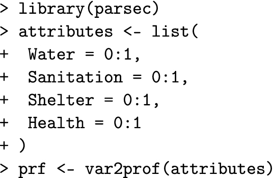
In this appendix, we report the R code used to elaborate the example pertaining to child well-being in the Democratic Republic of Congo (Sect. 4). Readers may easily replicate the computations and use the following scripts for further applications.

• 1. Definition of the set of binary profiles.

  

• 2. Data reported in Table 9 are put into the data.frameCONGO (notice that the profiles in CONGO must be listed in the same order as in prf).

• 3. Application of the F-FOD procedure.

  

• 4. Function FFOD returns several results (e.g. the matrix $\Delta$ of dominance degrees and the cover matrices of the $\alpha$-cut posets) and feeds the function rank_stability, which computes in each $\alpha$-cut poset the average rank of each profile and the rank intervals with the chosen least coverage probability.

  

• 5. The graphs shown in Fig. 9 are finally produced by:

  

Running the above computations took 5.46 secs on a pc equipped with Intel(R) Core(TM) i7-3632QM CPU @ 2.20GHz, 8GB ram, Windows 10, R version 3.4.3 and R Studio 1.1.382.

References

Annoni, P., Fattore, M., & Bruggemann, R. (2011). A multi-criteria fuzzy approach for analyzing poverty structure. Statistica & Applicazioni - Special Issue, 2011, 7–30.
Arcagni, A. (2017). PARSEC: An R package for partial orders in socio-economics. In M. Fattore & R. Bruggemann (Eds.), Partial order concepts in applied sciences. Cham: Springer.
Arndt C., Distante R., Hussain M. A., Østerdal P. L., Pham L. H., & Ibraimo M. (2012). Ordinal welfare comparisons with multiple discrete indicators: A first order dominance approach and application to child poverty, WIDER Working Paper, 2012/36, ISBN 978-92-9230-499-7.
Arndt, C., Vincent, L., & Kristi, M. (2014). Multi-dimensional poverty analysis for Tanzania: First order dominance approach with discrete indicators, WIDER Working Paper, 2014/146, ISBN 978-92-9230-867-4.
Bandler, W., & Kohout, L. (1988). Special properties, closures and interiors of crisp and fuzzy relations. Fuzzy Sets and Systems, 26, 317–331.
Bruggemann, R., & Patil, G. P. (2011). Ranking and prioritization for multi-indicator systems. New York: Springer.
Bubley, R., & Dyer, M. (1999). Faster random generation of linear extensions. Discrete Mathematics, 201, 81–88.
Davey, B. A., & Priestley, B. H. (2002). Introduction to lattices and order. Cambridge: CUP.
De Baets, B., & De Meyer, H. (2003). Transitive approximation of fuzzy relations by alternating closures and openings. Soft Computing, 7, 210–219.
De Loof, K., De Baets, B., & De Meyer, H. (2006). Exploiting the lattice of ideals representation of a poset. Fundamenta Informaticae, 71(2–3), 309–321.
De Loof, K., De Baets, B., & De Meyer, H. (2008). Properties of mutual rank probabilities in partially ordered sets. In J. W. Owsinski & R. Bruggemann (Eds.), Multicriteria ordering and ranking: Partial orders, ambiguities and applied issues. Warsaw: Polish Academy of Sciences.
De Loof K. (2010). Efficient computation of rank probabilities in posets. Ph.D. dissertation.
De Meyer, H., Naessens, H., & De Baets, B. (2004). Algorithms for computing the min-transitive closure and associated partition tree of a symmetric fuzzy relation. European Journal of Operational Research, 155, 226–238.
Dushnik, B., & Miller, E. W. (1941). Partially ordered sets. American Journal of Mathematics, 63(3), 600–610.
El Sayed T., Zahran A. R. (2016). Multidimensional almost dominance: Child wellbeing in Egypt Social Indicators Reearch, https://doi.org/10.1007/s11205-016-1541-9.
Fattore, M. (2016). Partially ordered sets and the measurement of multidimensional ordinal deprivation. Social Indicators Research, 128(2), 835–858. https://doi.org/10.1007/s11205-015-1059-6.
Fattore, M., & Arcagni, A. (2016). A reduced posetic approach to the measurement of multidimensional ordinal deprivation. Social Indicators Research, 136(3), 1053–1070. https://doi.org/10.1007/s11205-016-1501-4.
Fattore, M. (2017). Functionals and synthetic indicators over finite posets. In M. Fattore & R. Bruggemann (Eds.), Partial order concepts in applied sciences. Springer AG: Cham.
Hussain, M. A., Jørgensen, M. M., & Østerdal, P. L. (2016). Refining population health comparisons: A multidimensional first order dominance approach. Social Indicators Resarch, 129, 739–759.
Lee, K. H. (2005). First course on fuzzy theory and applications. Berlin: Springer.
Mishra, S. U., & Shukla, V. (2016). Welfare comparisons with multidimensional well-being indicators: An Indian illustration. Social Indicators Research, 129, 505–525. https://doi.org/10.1007/s11205-015-1117-0.
Nanivazo, M. (2015). First order dominance analysis: Child wellbeing in the Democratic Republic of Congo. Social Indicators Research, 122, 235–255.
Neggers, J., & Kim, S. H. (1998). Basic posets. Singapore: World Scientific.
Olu A., Afeikhena T. J., Olanrewaju O., Kristi M., & Olufunke A. A. (2014). Multidimensional poverty in Nigeria: First order dominance approach, WIDER Working Paper, No. 2014/143.
Peeva, K., & Kyosev, Y. (2004). Fuzzy relational calculus. Singapore: World Scientific Publishing.
Permanyer I., Hussain M. A. (2017). First order dominance techniques and multidimensional poverty indices: An empirical comparison of different approaches, Social Indicators Research https://doi.org/10.1007/s11205-017-1637-x.
R Core Team (2017). R: A language and environment for statistical computing, R foundation for statistical computing, Vienna, Austria. https://www.R-project.org/. Accessed 30 Nov 2017.
Schröder. (2002). Ordered sets. An introduction. Boston:Birkäuser.
Siersbæk, N., Østerdal, P. L., & Arndt, C. (2016). Multidimensional first-order dominance comparisons of population wellbeing. In C. Arndt & F. Tarp (Eds.), Measuring poverty and wellbeing in developing countries. Oxford: Oxford University Press.
Szpilrajn, E. (1930). Sur l’extension de l’ordre partiel. Fundamenta Mathematicae, 1(16), 386–389.
Author information
Authors and Affiliations
Corresponding author