Abstract
Anthropogenic impacts have shifted aquatic ecosystems far from prehistoric baseline states; yet, understanding these impacts is impeded by a lack of available long-term data that realistically reflects the organisms and their habitats prior to human disturbance. Fish are excellent, and largely underused, proxies for elucidating the degree, direction and scale of shifts in aquatic ecosystems. This paper highlights potential sources of qualitative and quantitative data derived from contemporary, archived and ancient fish samples, and then, using key examples, discusses the types of long-term temporal information that can be obtained. This paper identifies future research needs with a focus on the Southern Hemisphere, as baseline shifts are poorly described relative to the Northern Hemisphere. Temporal data sourced from fish can improve our understanding of how aquatic ecosystems have changed, particularly when multiple sources of data are used, enhancing our ability to interpret the current state of aquatic ecosystems and establish effective measures to safeguard against further adverse shifts. The range of biological, ecological and environmental data obtained from fish can be integrated to better define ecosystem baseline states on which to establish policy goals for future conservation and exploitation practices.
Introduction
Global changes to marine and freshwater ecosystems caused by anthropogenic activities have led to widespread impacts to many species of fish. To understand present and estimate future conditions of aquatic environments, as well as potential adaptive responses of the aquatic fauna, an understanding of historical trends and conditions of baseline states is needed (Hobday and Lough 2011; Higgs et al. 2014; Schwerdtner Máñez et al. 2014). Moreover, given that aquatic ecosystems provide habitat for exploited wild fish populations, the dual interests of exploitation and conservation are met by restoring and preserving the structure and function of aquatic habitats to their baseline state (Pitcher 2005). The reconstruction of ecosystem baseline states becomes the basis for the concept “Back to the Future” (Pitcher 2001), whereby, baseline states provide benchmarks on which to establish policy goals for future conservation and exploitation practices (Fig. 1). While shifts in baseline states may result in the formation of novel future ecosystems that lack historical analogs (Williams and Jackson 2007; Hobday 2011), developing an understanding of biological response to ecosystem change is still valuable to develop effective conservation strategies (Chambers et al. 2013; Hobday and Evans 2013).

Diagram illustrating the “Back to the Future” concept for the restoration of past aquatic ecosystems. The perfect circle on the left represents the prehistoric baseline state of an ecosystem. Through time, shifts in the state of the ecosystem results in progressively imperfect circles, where the diameter and complexity of the circle are inversely related to biodiversity and internal complexity. Timelines of representative species (ellipses) are shown (as solid horizontal lines), where ellipse size represents relative abundance. Crosses indicate species extinctions and arrows indicate the introduction of non-native species (depicted as squares and triangles). A range of potential alternative future ecosystems (i.e. restoration goals) are drawn to the right; however, note that due to natural variation and alteration of ecosystem function, the prehistoric baseline state is unlikely be perfectly replicated. Figure adapted from Pitcher (2001)
For the purpose of this paper, we define prehistoric ecological and environmental ‘baseline states’ as those in existence prior to human disturbance, as we acknowledge that ancient Indigenous cultures impacted aquatic ecosystems and the associated native fish populations (e.g. Leach and Davidson 2000; Long et al. 2014). Following this definition, a ‘shift’ from a baseline state refers to the modification or degradation of the structure and function of an ecosystem as a result of anthropogenic impacts. Hence, time scales on which prehistoric baseline states were present will differ dependant on geographic location. Natural variation is also likely to act synergistically with anthropogenic mediated impacts, contributing to shifts in baseline states. In this way, baseline shifts in aquatic ecosystems are not solely due to exploitation and habitat modification, but can also be attributed to changes in atmospheric or hydrological conditions.
Our understanding of baseline states is often misrepresented due to the psychological tendency to relate changes to an ecosystem against a prior baseline that represents a significantly altered form of the original state of the ecosystem (Pauly 1995; Hobday 2011). In this way, long-term and significant changes to the environmental structure and ecological functioning of an ecosystem will be unintentionally disguised, undermining efforts to restore ecosystems to (near-) prehistoric baseline states (Pauly 1995; Dayton et al. 1998). Thus, in order to more accurately represent shifts in baseline states, information from earlier time periods are required to reconstruct conditions that more realistically reflect the organisms and their habitats prior to disturbance (Jackson et al. 2001; Pitcher 2001; Higgs et al. 2014). Dependent on the availability (and quality) of archival information as well as differing levels of temporal resolution, time scales for which ecosystem baselines may be reconstructed will differ (Fig. 2).

The period of modern scientific data (shaded area) approximately spans the last 50–100 years. The integration of data derived from multiple sources extends the temporal breadth of data sets (and the resultant reconstructions of baseline states) over several 1000 years into the past; however, palaeontological and archaeological data may not easily be temporally resolved (dashed lines). The availability of data from each source varies temporally (solid line); however, it is likely that temporal discontinuities exist, such that data availability is not just a function of time (as depicted here) and subject to a suite of limiting factors specific to each source of data (refer to text). Figure adapted from Lotze and Worm (2009)
A suite of biological and ecological data can be gleaned from an individual fish (Fig. 3; Table 1). Hard parts of fish (e.g. ear bones or otoliths, vertebrae, scales, as well as fin spines and rays) are useful for elucidating shifts in biological and ecological processes and the physicochemical environment. Quantification of environmentally derived chemical concentrations incorporated into these hard parts provide a temporal record of the environmental history of an individual that can be matched to annual growth increment patterns (Elsdon et al. 2008). Incremental patterns of hard parts also provide a means to reveal the age and growth rates of fish. These structures are sufficiently robust to be found in sedimentary deposits, archaeological sites and the fossil record, providing temporal records extending back hundreds, thousands, and even millions of years (Fig. 2). Due to the long-held cultural significance of fish, as well as the commercial and recreational importance of many species, historical accounts and archived collections of fish are also relatively comprehensive over extended time scales (Wandeler et al. 2007; Humphries and Winemiller 2009; Morrongiello et al. 2012).

Examples of ecological information that can be obtained from fish to detect shifts in baseline states (note various components not to scale): (a) otoliths, (b) vertebrae, (c) fin spines and rays, (d) skin, (e) flesh, (f) viscera, (g) scales, (h) teeth and skeletal remains (jaw image used with permission from R. Baldock), and the (1) whole organism, (2) body dimensions
The overall aim of this paper is to examine the potential use of fish to establish prehistoric baseline states against which to judge present and potential future conditions of ecosystems and the fish species reliant upon them. This review first highlights potential sources of data associated with fish and then details the types of long-term biological and environmental information that can be obtained. Knowledge gaps and potential future research directions are subsequently discussed. Due to the scope of this review, we do not present an exhaustive list, but a selection of examples from the literature. We focus on Southern Hemisphere examples, which remain poorly described relative to the ‘classic’ Northern Hemisphere examples of shifted baseline states in aquatic ecosystems, such as historic declines in Atlantic cod abundances. However, where Southern Hemisphere examples were not available, we have presented examples from the Northern Hemisphere.
Sources of data
Here, we briefly describe the types of data sources associated with fish for detecting shifts in baseline states, their temporal and spatial scales (Fig. 2), and limitations of each data source.
Palaeontological data
Palaeontological records, prior to human influence, provide the ultimate prehistoric baseline to place current changes into context. Preserved fish remains and fossilised impressions left on geological substrates are useful tools to explore ancient fish distributions, abundances and community structure, as well as speciation and extinction (Baumgartner et al. 1992; Finney et al. 2010). Variations in fish populations and taxa across time and space can be further used to infer past climate and oceanographic conditions (Monsch 1998; Girone and Nolf 2009). The chemical record locked within body fossils can reveal information about past environmental conditions on finer temporal and spatial scales (Price et al. 2009), as well as fish movement, habitat use and metabolic rate (Schmitz et al. 1991; Carpenter et al. 2003; Price et al. 2009). Furthermore, data on growth rate, ontogenetic events and age have been obtained through the analysis of growth increments within fossil otoliths (Woydack and Morales-Nin 2001). Fossilised soft tissues, although extremely rare, provide insights into ancient diet (Wilby and Martill 1992) and reproductive strategies (Long and Trinajstic 2010).
A specific suite of environmental, biological and geochemical conditions is required to adequately preserve fossil remains (Donovan 2002); thus, the fossil record may under- or over-represent certain habitats, taxa, body parts, time periods and geographic regions. Taphonomic (fossilisation) processes that occur between death, preservation and subsequent discovery may affect the suitability of fossils for analyses. For example, a fish carcass may undergo post-mortem transport prior to final burial (e.g. Long and Trinajstic 2010), potentially confounding inferences derived from chemical analyses. The degree of diagenesis (alteration of the fossil’s original chemical and structural composition) can also affect the accuracy of chemical analyses (Schmitz et al. 1991; Zazzo et al. 2006) and the visualisation of growth increments in otoliths (Woydack and Morales-Nin 2001). Useful, well-preserved fossils are a relatively rare data source, but if acquired, are excellent for establishing baselines.
Archaeological data
Archaeological fish remains are confined to times of human habitation, which vary greatly among regions, and are frequently recovered from archaeological sites (e.g. Casteel 1976; Disspain et al. 2015). Hence, these remains reflect selective processes rather than direct representations of former fish populations (Reitz 2004). In addition, archaeological data may reflect populations impacted by human predation from Indigenous people, even at subsistence levels, and may not accurately represent pre-exploitation baselines (Mannino and Thomas 2002).
As with palaeontological samples, species identification and analyses of the chemical and chronological properties of fish remains (Disspain et al. 2015) enables more accurate and in-depth baseline data to be collected concerning fish species, size, age, habitat use and movement (Rose 1996; Van Neer et al. 2002; Balazik et al. 2010), as well as palaeoenvironmental conditions (Wurster and Patterson 2001; Zazzo et al. 2006). However, consideration of taphonomic processes (Zohar et al. 2008), degree of preservation (Bird 1992; Przywolnik 2002), and collection techniques (Vale and Gargett 2002; Nagaoka 2005) are similarly required as each may contribute to the loss of material from the record and influence final interpretations of ecological baselines (Zohar et al. 2008). Archaeological fish remains are also powerful aids to understanding human behaviour and exploitation of the environment; analyses can explore seasonal exploitation patterns and the movement of people within the land, methods of capture, diet, food processing methods, trade routes and cultural practices or preferences (Colley 1990; Higham and Horn 2000).
Historical records
A range of data sources generally categorised as historical records are associated with periods of exploration, settlement and the expansion of communities. This past information can be used to profile the development of fisheries, changes in fishing gear or effort, as well as fluctuations in catch quantities and composition (Klaer 2001; Parsons et al. 2009). These sources can be difficult to reconcile, but are valuable in understanding long-term patterns of resource use, because they span multiple ecological scales. Historical references can also be combined with contemporary fisheries and ecological models to generate estimates of biomass or distribution prior to or in the early stages of exploitation (e.g. Rosenberg et al. 2005).
Anecdotes, including qualitative statements in journals or diaries of explorers and settlers, provide information on species occurrences prior to historical exploitation. Individual references can be directly used as observations (Jackson 1997; Hardt 2009) or coded into quantitative estimates of perceived abundance (Palomares et al. 2007; Fortibuoni et al. 2010). Alternative sources of anecdotal (qualitative) information include artwork and photographs (e.g. Fig. 4), which can compare changes in fish sizes over time (McClenachan 2009), and local restaurant seafood menus, which, over many consecutive years, may provide a useful proxy for understanding changes in fish populations (Van Houtan et al. 2013). The early development of legislation can indicate when and why governments became concerned about a species or area (Kirby 2004), as well as provide a detailed account of changes in the management of fisheries or human impacts.

Commercial catch of Murray cod (Maccullochella peelii), viewed across the foredeck of P.S. Mayflower (circa 1914) (The State Library of South Australia: Record No.: PRG1258/1/2600). Murray cod are no longer commercially fished in the River Murray and are listed as nationally threatened
Interviews of fishers have shown there can be generational differences between historical and contemporary fisheries including shifts in the composition and quantities of catches and changes in the location of fish or fisheries (Ainsworth et al. 2008; Thurstan et al. 2015). Minutes of evidence obtained during earlier parliamentary inquiries have also been used to retrospectively review past interviews (Thurstan et al. 2013). In some instances fisher knowledge has uncovered past local or species extinctions that would otherwise have been undetected (Sadovy and Cheung 2003; Turvey et al. 2010).
Challenges to the use of historical records are the ability to convert this information into a useable format, the uptake of these data in conventional models, and an often patchy or isolated temporal span; however, using multiple sources of data greatly reduces uncertainty. Historical records can validly be included into existing models to extend timelines, for example the mean trophic level of fisheries (Alleway et al. 2014) or population models to estimate past biomass (Rosenberg et al. 2005).
Commercial fisheries catch data
Commercial fisheries catch data (recorded landings, effort, and estimates of relative abundance) have been recorded for some fisheries since the mid-1800s, providing valuable insights into the use of fish resources and fishing activities (Lotze and Milewski 2004; Hobday and Evans 2013). Fisheries catch records provide continuous data sets of commercial fishing activities, with more recent data providing greater detail and finer spatial and temporal resolution, although this may vary among fisheries (Pinnegar and Engelhard 2008). Even over relatively short time periods (20–50 years), commercial fisheries data can reveal dramatic changes in fishing effort, declines in catches, and shifts in target species (Klaer 2001; Ferguson et al. 2013). However, estimated population abundances extrapolated from commercial catch data generally represent fish populations in an already impacted state (Jackson et al. 2001; Pinnegar and Engelhard 2008; Humphries and Winemiller 2009).
Due to the fisheries-dependent nature of these data, there is a strong bias towards commercially exploited species. Data for incidentally caught species are generally spatially and temporally patchy due to poor reporting (Stobutzki et al. 2001). As with target species, catch records for non-target species likely represent population abundances and distributions in an already impacted state; nevertheless, fisheries data are still invaluable in tracking relative changes in abundances (Zeller and Pauly 2005).
The collation of long-term data sets from multiple fishery agencies and across multiple time periods requires standardisation to minimise the confounding effects of biological variability and changes in fishing practices (e.g. changing quotas, methodological advances: Bishop 2006). Increasing the catchability of species will erroneously suggest an apparent abundance in fish resources and underestimate population shifts (Quinn and Dersio 1999; Bishop 2006). However, statistical approaches can standardise catch data (Quinn and Dersio 1999; Hobday and Evans 2013).
Experimental and monitoring data
Ecological research in the aquatic environment, including laboratory experimentation, field collections and observations, and environmental monitoring, has a relatively short history, extending back only 100 years or so (Jackson 1997). Nevertheless, such quantitative data covers a period in time that is marked by an intensification of anthropogenic pressure on the aquatic environment (Jackson et al. 2001). Increased understanding of the correlative and/or causative influence of extrinsic factors on key biological and ecological processes provides a framework on which to interpret and calibrate older, qualitative data sources (Jackson et al. 2001; Hobday and Evans 2013). For example, experimental data linking water chemistry with otolith chemistry (Elsdon and Gillanders 2002, 2005) has been used to reconstruct the environmental conditions experienced by fish in the mid- to late-Holocene (Disspain et al. 2011).
Monitoring of fisheries resources and aquatic ecosystems, including assessments of biodiversity, stock biomass, and population structure (i.e. genetic structuring, size and age frequencies), provide key measures of the health of aquatic environments at a given point in time (e.g. Babcock et al. 2010). Discontinuities may exist in the timing and spatial coverage of monitoring data, as well as in the methodologies used to obtain the data between sampling periods, resulting in multiple short-term datasets. However, the value of these quantitative data cannot be discounted for investigating and tracking environmental change through time.
Baseline information obtained from data sources
The various data sources associated with fish (refer to “Sources of data” section above) can be broadly categorised as providing baseline information on (1) fish biology and ecology and on (2) environmental conditions. Using some key examples from the literature, we highlight how data sourced from fish have detected biological, ecological and environmental baseline shifts.
Fish biology and ecology
Diversity, distribution and abundance
A range of data sources provides insights into how fish diversity, abundance and distribution have shifted over decadal, centennial and even millennial time scales. Many key examples of baseline shifts in the aquatic environment demonstrate changes in fish abundance, largely focusing on exploited species linked to overfishing (Pauly 1995; Pitcher 2001; Pinnegar and Engelhard 2008). These fishery-related studies are primarily focused on periods relevant to European colonisation and/or the Industrial Revolution and the associated onset of large-scale commercial exploitation (Jackson et al. 2001; Pinnegar and Engelhard 2008). During this period, examples exist of declines in fish abundance, generally in large bodied species that are slow-growing and late-maturing, for example Murray cod (Maccullochella peelii) (Rowland 1989; Humphries and Winemiller 2009; Alleway et al. 2016) and Australasian snapper (Chrysophrys auratus) (Parsons et al. 2009; Thurstan et al. 2016), with the latter species experiencing an estimated 80 % reduction in biomass in the Hauraki Gulf/Bay of Plenty region of northern New Zealand (Gilbert 1994). Declines in such species also result in global or localised extinctions, altering community structure and diversity (Fortibuoni et al. 2010; Turvey et al. 2010; Last et al. 2011). However, substantial variation observed in ancient fish abundances prior to industrial-scale fishing have been linked with climatic cycles (Finney et al. 2010). For example, a 1700 year long reconstruction of fish scale deposition in sedimentary cores, found that sardine (Sardinops sagax) and anchovy (Engraulis mordax) populations in California had undergone regular 60–100 year cycles of collapse and recovery (Baumgartner et al. 1992). To our knowledge, such temporally extensive reconstructions of a Southern Hemisphere fish species have not been undertaken.
More recently, scientists have linked long-term unidirectional shifts in fish distribution and abundance to anthropogenic climate change (Holbrook et al. 1997; Perry et al. 2005). Such shifts are usually associated with increases in water temperature and the subsequent expansion, extension or contraction of a species natural distributional range (Madin et al. 2012). One of the most well-documented examples in the Southern Hemisphere relates to the poleward shift of 45 fish species in south-east Australia, a notable climate change hotspot (Last et al. 2011). Although anecdotal evidence exists in relation to temperature-induced range shifts (Gartside et al. 1999), accurately identifying the causal links associated with changing fish distributions is difficult due to the paucity of historical baseline data (Booth et al. 2011; Madin et al. 2012). Existing decadal-scale scientific surveys enable fish distributional patterns to be tracked (Stuart-Smith et al. 2010), but they cover only comparatively short time scales and are expensive to implement. Recently, online citizen science databases have provided an on-going record of fish diversity, distribution and abundance, and if maintained will provide a valuable insight into how these climate-related baselines are shifting from today into the future (e.g. http://www.redmap.org.au: see Last et al. 2011).
Undoubtedly, alterations in baseline fish diversity, abundance and distribution have occurred due to anthropogenic stressors such as invasive species, pollution and habitat modification (Bax et al. 2003; Shahidul Islam and Tanaka 2004). However, few studies have examined long-term changes in fish populations in association with these stressors, warranting further investigation.
Migration and connectivity
Although wholesale shifts in fish distributions are relatively well documented, long-term alterations in migration and connectivity patterns are not well known, impeding our ability to detect them through time. Conventional tag and recapture data as well as direct observations of fish movements can provide a measure of fish migration. Monitoring fishways on the River Murray in Australia showed a drastic decline of native species moving through the river system, including reductions of 95 % in silver perch (Bidyanus bidyanus), 96 % in Murray cod, and 51 % in golden perch (Macquaria ambigua) spanning 47 years (Mallen-Cooper and Brand 2007). These observational data can also highlight phenological shifts in the timing of migratory events. While no examples exist for Southern Hemisphere fish (Chambers et al. 2013), there are numerous examples in the Northern Hemisphere, particularly for salmonids (Poloczanska et al. 2013). For example, delays of up to 21 days in the seasonal timing of spawning migrations of Atlantic salmon (Salmo salar) have been observed over a 39 year period, and correlated to long-term changes in temperature and flow rates in several North American rivers (Juanes et al. 2004). In addition, these shifts in migration may be coincident with changing trends in life history patterns of fish. However, there are few instances where appropriate methods have been implemented over sufficiently extensive time periods to detect changes in migration and habitat use of fish.
Chemical (element and isotope) analyses of fish hard parts provide means of reconstructing migratory patterns over considerable time scales (Carpenter et al. 2003; Disspain et al. 2011). For example, elemental profiles in ancient otoliths may be contrasted against modern samples to examine changes in migratory patterns between collection periods. Hard part chemistry has also provided an understanding of meta-population structure with respect to interchange of adults and larvae between habitats (Bode et al. 2006).
Size and age structure
Data relating to fish body mass and length can be used to examine trends in the size frequency of a population or species over time. These types of data are valuable as they are relatively easy to source from records of commercial landings (e.g. Genner et al. 2010) and environmental monitoring (e.g. Bell et al. 1985), and effects of fishing on fish size are well understood (Rochet and Trenkel 2003; Jennings and Dulvy 2005). When contemporary records are combined with archaeological samples, a broad temporal record can be examined and shifts in the size frequency might be detected. For example, a decrease in large predatory fish assemblages in the Northern Hemisphere is attributed to fishing in the Roman period (Luff and Bailey 2000) and in the Southern Hemisphere by fishing from pre-European New Zealand Maori (Leach and Davidson 2000). Studies on more recent and shorter temporal periods are numerous (e.g. Ferguson et al. 2013) and can show effects of industrialised fishing on size classes of target species (Babcock et al. 1999; Dulvy et al. 2004). However, problems from size based techniques may arise from growth and age at size (i.e. length of fish is often used as a proxy for age) varying independently of fishing effort (Luff and Bailey 2000).
Information from growth increments within fish hard parts can provide an accurate measure of fish age when validated (Campana 2001), providing a powerful biological tool to measure temporal patterns of recruitment and the health of fish populations (Hsieh et al. 2006). Analysis of the selective effects of fishing on age structures has provided contrasting historical and contemporary data on a short-lived species, southern garfish (Hyporhamphus melanochir) from South Australia (Fowler and Ling 2010). Comparisons of the age structures from commercial catches during two periods, 50 years apart, indicate a decrease in the dominate age cohorts from 3+ and 4+ year olds to 1+ and 2+ year olds, implying a truncation in the population age structure. Over similar time scales, truncated age structures are also evident in longer lived species (Walsh et al. 2010; Stewart 2011). Reductions in age classes are concerning, as they can increase stock vulnerability to environmental change (Hsieh et al. 2006) and/or show a lack of recruitment success (Ferguson et al. 2008; Whitten et al. 2013). However, like size based studies, it is important to validate data because erroneous age information has been a factor in the over-exploitation of fish stocks; for example, initial underestimation of the length-at-age (and hence rates of growth and mortality) of orange roughy (Hoplostethus atlanticus) resulted in unsustainable harvesting of the species (Smith et al. 1995; Campana 2001).
Growth
Relative shifts in somatic growth rates provide a means of detecting changes in population abundance as a density dependent response to exploitation (Ziegler et al. 2007) and/or as a physiological response to changing environmental conditions (Neuheimer et al. 2011). Comparisons of growth curves (e.g. von Bertalanffy growth function, Gompertz growth function) provide evidence of changing growth rates through time (e.g. Fig. 5). These studies are largely fisheries-based and focused on exploited species. Hence, changes in growth rates are generally assumed to be the result of length-selective fishing mortality (Walker et al. 1998), but may also be attributed to environmental change (Cottingham et al. 2014). Comparisons of growth rates can be made among populations of fish sampled discontinuously through time and at broad spatial scales, allowing contemporary growth to be contrasted against estimates of growth derived from archaeologically sourced samples (Disspain et al. 2011). It must be noted that relative changes in growth (as depicted by growth curves) may be driven by exploitation and environmental variability, as well as sampling biases and other methodological considerations (Moulton et al. 1992; Walker et al. 1998). These factors, working independently or in combination, may inflate real shifts in growth rates, necessitating critical assessments of the data when drawing comparisons among multiple disparate studies.

Comparisons of von Bertalanffy growth curves for southern garfish (Hyporhamphus melanochir) in southern Australia, sampled 47 years apart. Solid line depicts data for garfish sampled in 1954/55 (n = 2234) (Ling 1958), and the dashed lines show data for garfish sampled between 1997 and 2000 (n = 2079) (Ye et al. 2002). Reported sizes at first maturity are also indicated (gray triangle)
Alternate approaches to assessing changes in somatic growth over time are based on annual growth of an individual either through physical measurements of the body (i.e. lengths and weights) or via a proxy (i.e. hard parts). Assessments of length-at-age dynamics are capable of detecting shifts in growth and have been used to document year-to-year changes in growth over multiple decades (e.g. Whitten et al. 2013). Even over relatively short periods of time (i.e. 10 years), significant increases in growth have been observed in a commercially targeted population of long-lived banded morwong (Cheilodactylus spectabilis) from eastern Tasmania, Australia (Ziegler et al. 2007). Given that the species can live up to 95 years (Thresher et al. 2007), growth increases (i.e. 13 % in the 3-year age cohort) in a 5–10 year period suggest a density-dependent phenotypic shift in the demography of the population (independent of genotypic influence) (Ziegler et al. 2007).
Sclerochronological analyses, the examination of growth increment patterning in hard parts, provides an excellent proxy record of growth, assuming that for a given species a relationship exists between growth of the hard part (i.e. width of the growth increments) and somatic growth (Morrongiello et al. 2012). Sclerochronology and measured changes in length-at-age are advantageous over direct comparisons of growth curves, as they provide time resolved chronologies of growth that extend back over decadal and centennial time scales. This facilitates assessments of long-term correlations to time series data, such as recruitment indices, catch statistics and instrumental environmental measures (Morrongiello et al. 2014; Morrongiello and Thresher 2015), allowing the causative effects of environment and human induced pressures on fish populations to be disentangled. However, physiological regulators of growth, such as species-specific temperature optima, may decouple relationships between somatic and hard part growth potentially confounding changes in growth rates (Neuheimer et al. 2011).
Currently, the most extensive sclerochronologies developed from aquatic environments are based on increment patterning in coral skeletons and bivalve shells, with otolith-based chronologies starting to become more common (Morrongiello et al. 2012). For example, in the Southern Hemisphere, a number of recent studies have investigated growth patterns in freshwater, estuarine and marine fish over centennial and decadal time scales, linking fluctuations in growth to environmental variation (Morrongiello et al. 2011; Gillanders et al. 2012; Doubleday et al. 2015). While sclerochronologies enable the exploration of inter-annual changes in mean population growth, correlations between growth and environmental parameters facilitate the predictive modelling of future growth under climate change scenarios (Morrongiello et al. 2011). For example, using sclerochronological approaches, an annually resolved 50 year chronology (1952–2003) for western blue groper (Achoerodus gouldii) from south-western Western Australia, was positively correlated with regional sea surface temperature (Rountrey et al. 2014). Based on this observed correlation, additive models were used to predict otolith growth and body size under future warming scenarios (i.e. a fish 20-years of age in 2099 would have a body size approximately 5 % larger than a 20-year old fish in 1977).
Reproduction
Changes in rates of growth often coincide with shifts in the reproductive biology of species (e.g. Fig. 5). For example, selective pressure (i.e. from fishing or unfavourable conditions) may encourage rapid growth and the early onset of sexual maturity due to selection for that trait (genetic) or compensatory responses, such as density dependence (Trippel 1995). Increased growth in Tasmanian banded morwong corresponded with a decline in female age at 50 % maturity (Ziegler et al. 2007). Similarly, temporal changes in growth of gummy shark (Mustelus antarcticus) from south-eastern Australia, coincided with changes in the length-at-maturity (Walker et al. 1998; Walker 2007). These changes were assumed to be in response to increasing fishing mortality such that increased fishing intensity resulted in the early onset of maturity (Walker 2007). However, delineating causes of early maturation is difficult in many species, since changes to the timing of maturity may be constrained by species-specific responses to both genetic and compensatory factors (Trippel 1995). The use of maturation reaction norms, describing the probability of fish maturity as a function length, has been used to assess temporal change in the size and length of maturation of fish (Heino et al. 2002), and facilitate exploration of genotypic and/or phenotypic influences on changes in the time to maturity. Comparisons of reaction norms for maturation of the Western Australian estuary cobbler (Cnidoglanis macrocephalus) sampled at two periods, 20 years apart, indicated a significant decrease in the length- and age-at-maturity over time (Chuwen et al. 2011). The observed shift in the maturation reaction norm for C. macrocephalus, independent of growth, which remained stable through time, implies that changes in the length- and age-at-maturity represent a genotypic response to historic fisheries pressure on the population.
In the absence of direct observations of the reproductive state of fish, stable carbon (δ13C) and oxygen (δ18O) isotopes in fish hard parts may provide some utility in quantifying changes in the timing of sexual maturity (Schwarcz et al. 1998; Begg and Weidman 2001). However, these shifts may be confounded by fluctuations in ambient environmental concentrations and therefore require further exploration (Schwarcz et al. 1998).
Diet and food web dynamics
Studies examining dietary shifts in fish have contrasted dietary patterns (e.g. stomach content analyses) over relatively short time periods (decades) to better aid in detecting shifts in the complexity of food webs and the reduction of the number of trophic levels present in aquatic ecosystems; though we found few examples of such studies (and none representative of the Southern Hemisphere). These studies have documented significant shifts in the prey composition and relative importance of targeted species in the diets of predatory species (Overholtz et al. 2000; Feyrer et al. 2003). Changes in prey exploitation largely reflect changes in abundances of prey species through time and provide insights into altered food web dynamics (Overholtz et al. 2000).
Isotopic signatures preserved within the hard parts of fish have been recently recognised as valuable proxies of fish diet and trophic position over long temporal scales. Nitrogen isotopes (δ15N) within ancient midden otoliths revealed the trophic position of four fish species living in the Gulf of California 1500–5000 years ago based on the well-described and predictable relationship between trophic position and δ15N values, traditionally analysed in soft tissue (Rowell et al. 2010). Validation studies have also shown the potential of δ13C and δ15N isotopes, specifically within the organic component of the otolith, as powerful tools for reconstructing dietary and trophic histories (McMahon et al. 2011; Grønkjær et al. 2013). Furthermore, a global meta-analysis of otolith δ13C values measured in 60 fish species found that otolith δ13C values among species were consistently explained by an index of aerobic swimming capacity (Sherwood and Rose 2003). These findings suggest that δ13C values in otoliths could be used to reconstruct historical changes in aerobic activity, foraging patterns and food web dynamics in fish. In addition to isotopic records, historical dietary records of fish could also be used to examine shifts in diet and food web dynamics, as well as the stomach contents of preserved or fossilized specimens (although the latter is exceedingly rare: see Wilby and Martill 1992).
Genetic diversity
Archived and preserved fish remains provide valuable sources of DNA that represent genetic signatures of fish populations from decades or centuries past (Wandeler et al. 2007), providing insights into genotypic shifts in populations that are under a range of selective pressures (e.g. genotype-selective fishing mortality) (Hauser et al. 2002; Swain et al. 2007). A review of the suite of genetic methodologies is not within the scope of this paper and have been covered elsewhere (e.g. Nielsen and Hansen 2008). Placing population genetic studies in a historic context is becoming common, and such studies have identified the extinction or replacement of native populations (and their genetic composition) with introduced lineages (e.g. Nock et al. 2011).
On ecological time scales, comparisons of genetic variation within fish populations have shown temporal declines in genetic diversity and decreased heterozygosity for exploited species of fish, such as the orange roughy (Smith et al. 1991) and Australasian snapper (Hauser et al. 2002). Decreased genetic diversity may also result in a reduction of effective population sizes (Nielsen et al. 1997; Nielsen and Hansen 2008). The application of seven microsatellite markers obtained from historical and contemporary scale collections of Australasian snapper has helped to explain demographic declines in abundance, which resulted in 25 % decline in a New Zealand population of fished snapper over 35 years (Hauser et al. 2002). In this way, temporal patterns of genetic diversity can be used to track trends in a population’s abundance. Assessments of genetic diversity have also demonstrated selection at the molecular level, with the pantophysin (Pan I) locus in gadoid fishes of the Northern Hemisphere receiving the most attention (Nielsen and Hansen 2008). Selection at Pan I has been linked to shifts in growth phenotypes among populations and individuals (Case et al. 2005; Nielsen et al. 2007), suggesting fishing-induced selection of genotype frequencies (Jakobsdóttir et al. 2011). However, evidence shows that selection at Pan I may also have an environmental basis (Case et al. 2005). Genetic monitoring of allele frequencies may therefore enable the assessment of adaptive responses to exploitation and/or environmental change through repeated analyses of the same populations over time.
In spite of dramatic declines in fish abundances and changes in genetic diversity within populations, genetic population structure among spatially separated groups remains temporally stable in fishes based on archived and contemporary population comparisons (e.g. Bernal-Ramírez et al. 2003; Palstra and Ruzzante 2010), with a few exceptions (Østergaard et al. 2003). This suggests that applications of genetic data are best suited to detect temporal changes of within population genetic diversity and genotype expression.
Environmental conditions
Sclerochronology
Sclerochronologies can be used as proxies to reconstruct past climatic or oceanographic baselines as well as examine shifts in the growth of an organism over time (refer to “Growth” section above) (Thresher et al. 2007; Morrongiello et al. 2012; Thresher et al. 2014). When sclerochronology is correlated with environmental parameters (e.g. hydrologic, oceanographic, meteorologic) for a given area, long-term records of the seasonality of climate-growth relationships and the effects of temporal environmental variability can be deduced (Black et al. 2005; Gillanders et al. 2012). For example, historical annual growth rates over the last century were reconstructed from the otoliths of a suite of south-western Pacific fish species. These growth rates correlated with ocean temperature and exhibited significant changes based on depth (Thresher et al. 2007).
To further assess the environmental history of an area, elemental chemistry and stable isotope data collected from hard parts (see Table 2) can be coupled with the corresponding sclerochronological and environmental records of an area to produce a complete record of the environment that the fish has been exposed to over the course of its life time (Campana and Thorrold 2001; Gao and Beamish 2003; Black et al. 2005). This in turn allows realistic baselines, both biological and environmental, to be established and often, extended further back in time (Andrus 2011; Disspain et al. 2015).
Elements
Element concentrations in fish hard parts have been related to the surrounding ambient water chemistry (Schmitz et al. 1991; Wells et al. 2000). Thus, elemental quantification provides a means of describing the environmental histories of fish, as well as enabling the reconstruction of past environmental conditions experienced by fish (see Table 2 for description of elements relating to particular environmental parameters).
Time scales of environmental reconstructions based on elements in hard parts are restricted by the longevities of the fish species, with some individuals living over 100 years of age (e.g. Thresher et al. 2007), or the age of the samples. For example, comparisons of mean manganese (Mn) concentrations in Neolithic otoliths of Baltic cod were used to infer exposure to hypoxic conditions over a millennial time scale (Limburg et al. 2011).
The migratory nature of fish, both vertically and horizontally, may confound efforts to reconstruct past environmental conditions (Campana and Thorrold 2001). For example, element analysis in archaeological otoliths of mulloway (Argyrosomus japonicus) detected irregular patterns of barium (Ba):Ca, suggesting either considerable environmental changes in the Murray River system over time or frequent movements between freshwater and saltwater habitats (Disspain et al. 2011). Estimates of previous riverine conditions from archaeologically derived otoliths of Murray cod suggest the species was exposed to significant fluctuations in temperature and salinity prior to the development of the barrages and water management (Disspain et al. 2012).
Isotopes
A range of isotopes have been used to reconstruct past climates and environmental conditions from archaeological and modern calcium carbonate remains of fish (see Table 2). Although many of these isotopes are potentially applicable for use in fish, δ18O, 87Sr/86Sr and radiocarbon (14C) are the mostly widely used to date. Although isotopes have been measured in a range of fish hard parts, caution is suggested around the use of skeletal bone for isotopic analyses, as isotopic content is likely to degrade after death. Other hard parts are thought to be less susceptible to changes in isotopic ratios following death, but little research on diagenetic changes has been conducted (but see Lubinski 1996; Andrus and Crowe 2002).
Fish, like other aquatic organisms, precipitate δ18O into calcium carbonate structures as a function of water temperature and ambient water δ18O content. The latter may vary as a function of salinity in coastal waters, since the δ18O of water reflects evaporation, condensation, continental runoff and water mixing (Andrus 2011). If there is a strong seasonal temperature gradient, but little variation in salinity, then profiles of δ18O across otoliths (for example) may be used to reflect past temperatures (Andrus 2011). Similarly, if there is little variation in temperature but marked changes in precipitation, then δ18O may reflect changes in salinity. Therefore, where there is no a priori knowledge of δ18O of water, as for midden samples, it is difficult to assign temperatures or salinity (Andrus 2011). Modern experimental studies are generally required to validate the use of δ18O for reconstructing past environments. Such studies indicate that variation occurs on a species-by-species basis suggesting a need for many proxy validation studies (Thorrold et al. 1997; Elsdon and Gillanders 2002). Clumped isotope geochemistry, or the state of ordering of rare isotopes, represents a means of overcoming the lack of information on palaeo δ18O of water, thereby providing a palaeothermometer. In the case of carbonates, growth temperatures are based on the differences in bonds between 13C and 18O within the same carbonate ion group (Eiler 2011). Further information on clumped isotope geochemistry is provided in Ghosh et al. (2006) and Eiler (2007). This proxy for temperature has been validated for six species of fish spanning a latitudinal gradient (Ghosh et al. 2007), but has yet to be applied beyond use on modern day fish.
Strontium isotopes can also be used to study salinity through time but are restricted to low salinity waters. The 87Sr/86Sr ratio of seawater has essentially remained the same for the past 400,000 years (0.709) and is similar across the world’s oceans, whereas the Sr isotopic composition of river water reflects the 87Sr/86Sr of the bedrocks in the catchment area (Ingram and Sloan 1992). Because otolith 87Sr/86Sr is primarily determined by ambient water chemistry, applications have largely been limited to modern day fish (e.g. Schmidt et al. 2014). Comparisons of Sr isotopes have been made between ancient fish remains and modern day water samples; however, most samples could not be assigned to a precise geographical locality, potentially indicating spatial heterogeneity within a lake, a dietary contribution or post-mortem alteration of Sr during fossilisation (Dufour et al. 2007).
Bomb radiocarbon (Δ14C) in the aquatic environment (Fig. 6) can be used as a high-resolution dating tool, an important tracer of water mass circulation and to more accurately model the global carbon flux (Kalish 1994; Grammer et al. 2015). Bomb radiocarbon is the deviation of a sample’s 14C/12C ratio from pre-industrial levels due to worldwide testing of thermonuclear weapons from the 1950s to the 1970s (Mahadevan 2001). The Δ14C “bomb pulse” has been readily assimilated into both fresh and seawater masses, as well as in hard parts of aquatic organisms (Fig. 6; Kalish 1993).

An example of a bomb radiocarbon curve in the aquatic environment: Δ14C (±1 SD) from the otoliths of known-age Australasian snapper (Chrysophrys auratus, gray circle) (Kalish 1993) and nannygai snapper (Centroberyx affinis, black circle) (Kalish 1995) over the time period 1918–1990. Measurements of Δ14C from hermatypic coral (diamond) samples in Fiji are presented for comparison (Toggweiler et al. 1991). The dashed box represents the period of significant increase of the Δ14C in the aquatic environment, with the 14C signal first detectable in Southern Hemisphere marine surface waters around 1958 and peaking in the 1970s
Levels of bomb radiocarbon in corals and bivalves have been used to trace water masses (Toggweiler et al. 1991; Schöne and Gillikin 2013). In contrast, fish hard parts have been underused for similar applications, with Δ14C primarily being investigated as a means of age validation. Regional Δ14C curves (as seen in Fig. 6) may be compared with other regional curves to examine how radiocarbon is responding temporally within a system. Levels of Δ14C in marine environments are also depth dependent and generally become lower with increasing depth; water masses can be distinguished relative to the amount of mixing occurring by depth and region (e.g. Grammer et al. 2015). Changes in the levels of Δ14C in the otolith cores of petrale sole (Eopsetta jordani) were correlated with strong, variable upwelling events in the California Current system along the western coast of the United States, but rates of upwelling through time were not estimated (Haltuch et al. 2013).
Discussion
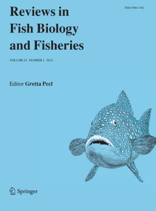
This review has demonstrated the potential for fish derived data to elucidate the degree, direction and scale of shifts in aquatic ecosystems. The range of biological, ecological and environmental data obtained from fish can aid in reconstructing ecosystem baseline states on which to establish benchmarks for restoration. This review sought to highlight baseline shifts in the Southern Hemisphere using data sources associated with fish, because there is a paucity of time series data spanning hundreds of years in comparison to the Northern Hemisphere (particularly Europe and North America) (Chambers et al. 2013). Fish can help bridge this knowledge gap by improving our understanding of changes to aquatic ecosystems, and as a result, improve management strategies to restore shifted baselines (see example in Fig. 7) (Schwerdtner Máñez et al. 2014). Continuing to focus on recent modification will perpetuate shifts away from prehistoric levels, and while this may slow change, it will ultimately fail to promote ecosystem restoration (Jackson et al. 2001; Pitcher 2001; Higgs et al. 2014).

Differences in fisheries management reference points based on historical and contemporary data. Stock biomass estimates (±SE) for Australasian snapper (Chrysophrys auratus) in the Hauraki Gulf/Bay of Plenty in New Zealand are based on historic fisheries and tagging data from two periods that are 24 years apart (Gilbert et al. 2000). Using a basic fisheries management scenario, catch allowances were established at 80 % of the estimated biomass for 1970 (shaded area) and 1994 (black area). Between the two time periods, catch allowances differed by 13.3 kilotons (kt), with the 1994 unfished biomass representing 5.5 % of the total estimated 1970s biomass. However, snapper in New Zealand have been exploited over the last 700 years (Parsons et al. 2009), with modelling of stock biomass to 1850 (circle) indicating a dramatic decline in local population abundance (Gilbert 1994). The photo shows a fisherman hauling a catch of snapper caught by Danish seining in the Hauraki Gulf off Auckland (circa 1940) (The Alexander Turnbull Library: Reference No.: PAColl-3060-067)
Returns to baseline states may be unrealistic, as natural variation and modification at every level in the ecosystem will hinder complete restoration (Pitcher 2005; Hobday 2011). Therefore, the real challenge for conservationists and resource managers, is to use time series data to better identify conditions and mechanisms that lead to dramatic shifts in baselines as well as understand patterns of organismal response to change, with the intent of predicting or safeguarding against further shifts (Connell et al. 2008; McClenachan et al. 2012; Schwerdtner Máñez et al. 2014).
In order to better utilise fish as a reliable source of long-term biological and ecological data, we suggest that future research be aimed at meeting a number of specific focus areas:
-
Apply archived fish samples to bridge temporal discontinuities in data sets (e.g. Fig. 2). Specific to the Southern Hemisphere, many sources of data (e.g. palaeontological and fisheries data) are deficient in availability relative to the Northern Hemisphere. This discrepancy has likely arisen due to the long histories of exploration, exploitation and scientific investigation of many Northern Hemisphere countries (Chambers et al. 2013; Litzow et al. 2016). Consequentially, there are few data sets of sufficient temporal breadth to demonstrate shifts in biological and ecological aquatic baselines in the Southern Hemisphere (e.g. phenological shifts: Chambers et al. 2013). However, many studies highlighted in this review ‘value add’ to data originally collected for other purposes; for example, using recreational fishing club records to detect changes in species abundance (Gartside et al. 1999). Encouraging a cultural shift in the broader research community to think beyond the ‘here-and-now’ will be fundamental in identifying and safeguarding data of potential value for assessing shifts in baseline states (Rivers and Ardren 1998). Historically museum and natural history collections have acted as hubs for the long-term centralisation and archiving of biological materials (Wandeler et al. 2007). However, research institutions are now collating biological samples (e.g. otoliths: Morrongiello et al. 2012) and efforts have been made to recover and conserve fisheries data (Zeller et al. 2005) with the intent of quantifying shifts in aquatic ecosystem states. Similarly, promoting a culture of data accessibility, for example data archiving as part of the publication process, will vastly improve access to published data (Vines et al. 2013). Yet, there are likely alternate forms of fish derived data that will become increasing accessible with methodological advancement (e.g. DNA extraction of fixed samples, environmental DNA profiling of lake varve samples).
-
Apply historical records in contemporary fisheries and ecological models (e.g. Rosenberg et al. 2005; Alleway et al. 2014). This review highlights the increasing number of studies assessing shifts in aquatic ecosystem baseline states, with the majority of examples provide here focused at changes in traits of a single species through time. However, understanding ecosystem-level shifts in baseline states requires the integration of biological data sets from multiple species exposed to shared abiotic and biotic ecosystem-level fluctuations, with evidence suggesting that studies using <30 biological time series are unlikely to detect ecosystem-level baseline shifts (Litzow et al. 2016). Similarly, understanding the broadscale influence of human activity on fisheries stocks or their structure can require the use of multiple data sources that may be seemingly disparate or from alternative disciplines, across greater lengths of time (e.g. Alleway et al. 2016). Therefore, future efforts into integrating these multiple sources of data from several species, coupled with environmental and chemical data sets will vastly improve our ability to examine shifts in baseline states at an ecosystem-level.
-
Investigate the chemical (elemental and isotopic) properties of fish hard parts as biochronometers of past environmental conditions (akin to bivalves and corals: Schöne and Gillikin 2013). This review has highlighted the potential sensitivity of fish hard part chemistries to a suite of ambient environmental conditions (e.g. Table 2) and biological parameters (e.g. reproductive timing, metabolism); however, few studies look to exploit these properties to investigate changes in aquatic environments or population phenologies. This may be due to issues in disentangling the relative influence of physiological and environmental effects on hard part chemistries, and therefore, requires manipulative experimentation that addresses the combined effects of physiology and environmental factors on the hard part chemical composition (e.g. Sturrock et al. 2014).
-
Investigate biological and ecological responses of fish to shared abiotic and biotic ecosystem-level fluctuations will aid in developing a mechanistic understanding of shifts from baseline states. Moreover, in situ monitoring provides information that is valuable for qualifying the current state of an ecosystem or population, but also provides data with which to model future scenarios and estimate prehistoric baseline states (Brander 2010). For example, assessing the potential for population recovery based on monitoring data from marine reserves (Babcock et al. 2010).
Conclusion
There is no doubt that humans have irreparably altered aquatic ecosystems, but understanding the extent and timing of these impacts is difficult, largely because suitable baseline data are lacking. This review has demonstrated that fish provide unique and largely underused tools to understand changes in the aquatic environment. They also have the potential to estimate baseline states from hundreds to thousands of years. This can best be achieved through the integration of data (both qualitative and quantitative) from across a suite of sources at both the organismal and ecosystem level. Ultimately, it is only by looking back through time that we will be able to adequately interpret the current state of aquatic ecosystems and establish effective measures to safeguard it from further adverse shifts.
References
Ainsworth CH, Pitcher TJ, Rotinsulu C (2008) Evidence of fishery depletions and shifting cognitive baselines in Eastern Indonesia. Biol Conserv 141:848–859
Alleway HK, Connell SD, Ward TM, Gillanders BM (2014) Historical changes in mean trophic level of southern Australian fisheries. Mar Freshw Res 65:884–893. doi:10.1071/MF13246
Alleway HK, Gillanders BM, Connell SD (2016) ‘Neo-Europe’ and its ecological consequences: the example of systematic degradation in Australia’s inland fisheries. Biol Lett 12:20150774. doi:10.1098/rsbl.2015.0774
Andrus CFT (2011) Shell midden sclerochronology. Quat Sci Rev 30:2892–2905. doi:10.1016/j.quascirev.2011.07.016
Andrus CFT, Crowe DE (2002) Alteration of otolith aragonite: effects of prehistoric cooking methods on otolith chemistry. J Archaeol Sci 29:291–299
Andrus CFT, Crowe DE, Romanek CS (2002) Oxygen isotope record of the 1997–1998 El Nino in Peruvian sea catfish (Galeichthys peruvianus) otoliths. Paleoceanography 17:5-1–5-8. doi:10.1029/2001PA000652
Babcock RC, Kelly S, Shears NT, Walker JW, Willis TJ (1999) Changes in community structure in temperate marine reserves. Mar Ecol Prog Ser 189:125–134
Babcock RC, Shears NT, Alcala AC, Barrett NS, Edgar GJ, Lafferty KD, McClanahan TR, Russ GR (2010) Decadal trends in marine reserves reveal differential rates of change in direct and indirect effects. Proc Natl Acad Sci 107:18256–18261
Balazik MT, Garman GC, Fine ML, Hager CH, McIninch SP (2010) Changes in age composition and growth characteristics of Atlantic sturgeon (Acipenser oxyrinchus oxyrinchus) over 400 years. Biol Lett 6:708–710
Barnes TC, Gillanders BM (2013) Combined effects of extrinsic and intrinsic factors on otolith chemistry: implications for environmental reconstructions. Can J Fish Aquat Sci 70:1159–1166. doi:10.1139/cjfas-2012-0442
Baumgartner T, Soutar A, Ferreira-Bartrina V (1992) Reconstruction of the history of Pacific sardine and northern anchovy populations over the past two millennia from sediments of the Santa Barbara Basin, California. Calif Coop Ocean Fish Investig Rep 33:24–40
Bax N, Williamson A, Aguero M, Gonzalez E, Geeves W (2003) Marine invasive alien species: a threat to global biodiversity. Mar Policy 27:313–323
Begg GA, Weidman CR (2001) Stable δ13C and δ18O isotopes in otoiiths of haddock Melanogrammus aeglefinus from the northwest Atlantic Ocean. Mar Ecol Prog Ser 216:223–233
Bell J, Craik G, Pollard D, Russell B (1985) Estimating length frequency distributions of large reef fish underwater. Coral Reefs 4:41–44
Bernal-Ramírez JH, Adcock GJ, Hauser L, Carvalho GR, Smith PJ (2003) Temporal stability of genetic population structure in the New Zealand snapper, Pagrus auratus, and relationship to coastal currents. Mar Biol 142:567–574. doi:10.1007/s00227-002-0972-9
Bird MK (1992) The impact of tropical cyclones on the archaeological record: an Australian example. Archaeol Ocean 27:75–86
Bishop J (2006) Standardizing fishery-dependent catch and effort data in complex fisheries with technology change. Rev Fish Biol Fish 16:21–38. doi:10.1007/s11160-006-0004-9
Black BA, Boehlert GW, Yoklavich MM (2005) Using tree-ring crossdating techniques to validate annual growth increments in long-lived fishes. Can J Fish Aquat Sci 62:2277–2284
Bode M, Bode L, Armsworth PR (2006) Larval dispersal reveals regional sources and sinks in the Great Barrier Reef. Mar Ecol Prog Ser 308:17–25
Booth DJ, Bond N, Macreadie P (2011) Detecting range shifts among Australian fishes in response to climate change. Mar Freshw Res 62:1027–1042. doi:10.1071/MF10270
Brander K (2010) Impacts of climate change on fisheries. J Mar Syst 79:389–402. doi:10.1016/j.jmarsys.2008.12.015
Campana SE (1999) Chemistry and composition of fish otoliths: pathways, mechanisms and applications. Mar Ecol Prog Ser 188:263–297
Campana SE (2001) Accuracy, precision and quality control in age determination, including a review of the use and abuse of age validation methods. J Fish Biol 59:197–242
Campana SE, Thorrold SR (2001) Otoliths, increments, and elements: keys to a comprehensive understanding of fish populations? Can J Fish Aquat Sci 58:30–38
Carpenter SJ, Erickson JM, Holland FD Jr (2003) Migration of a late Cretaceous fish. Nature 423:70–74. doi:10.1038/nature01575
Case RAJ, Hutchinson WF, Hauser L, Oosterhout CV, Carvalho GR (2005) Macro- and micro-geographic variation in pantophysin (Pan I) allele frequencies in NE Atlantic cod Gadus morhua. Mar Ecol Prog Ser 301:267–278. doi:10.3354/meps301267
Casteel RW (1976) Fish remains in archaeology and paleo-environmental studies. Academic, London
Chambers LE, Altwegg R, Barbraud C, Barnard P, Beaumont LJ, Crawford RJM, Durant JM, Hughes L, Keatley MR, Low M, Morellato PC, Poloczanska ES, Ruoppolo V, Vanstreels RET, Woehler EJ, Wolfaardt AC (2013) Phenological changes in the southern hemisphere. Plos One 8:e75514. doi:10.1371/journal.pone.0075514
Chuwen BM, Potter IC, Hall NG, Hoeksema SD, Laurenson LJB (2011) Changes in catch rates and length and age at maturity, but not growth, of an estuarine plotosid (Cnidoglanis macrocephalus) after heavy fishing. Fish Bull 109:247–260
Clarke LM, Thorrold SR, Conover DO (2011) Population differences in otolith chemistry have a genetic basis in Menidia menidia. Can J Fish Aquat Sci 68:105–114. doi:10.1139/F10-147
Colley SM (1990) The analysis and interpretation of archaeological fish remains. In: Schiffer MB (ed) Archaeological method and theory. The University of Arizona Press, Tucson, pp 207–253
Collingsworth PD, Van Tassell JJ, Olesik JW, Marschall EA (2010) Effects of temperature and elemental concentration on the chemical composition of juvenile yellow perch (Perca flavescens) otoliths. Can J Fish Aquat Sci 67:1187–1196. doi:10.1139/f10-050
Connell S, Russell B, Turner D, Shepherd S, Kildea T, Miller D, Airoldi L, Cheshire A (2008) Recovering a lost baseline: missing kelp forests from a metropolitan coast. Mar Ecol Prog Ser 360:63–72. doi:10.3354/meps07526
Cottingham A, Hesp SA, Hall NG, Hipsey MR, Potter IC (2014) Marked deleterious changes in the condition, growth and maturity schedules of Acanthopagrus butcheri (Sparidae) in an estuary reflect environmental degradation. Estuar Coast Shelf Sci 149:109–119. doi:10.1016/j.ecss.2014.07.021
Dayton PK, Tegner MJ, Edwards PB, Riser KL (1998) Sliding baselines, ghosts, and reduced expectations in kelp forest communities. Ecol Appl 8:309–322. doi:10.1890/1051-0761(1998)008[0309:SBGARE]2.0.CO;2
Devereux I (1967) Temperature measurements from oxygen isotope ratios of fish otoliths. Science 155:1684–1685. doi:10.1126/science.155.3770.1684
Dissard D, Nehrke G, Reichart GJ, Bijma J (2010) Impact of seawater pCO2 on calcification and Mg/Ca and Sr/Ca ratios in benthic foraminifera calcite: results from culturing experiments with Ammonia tepida. Biogeosciences 7:81–93
Disspain M, Wallis LA, Gillanders BM (2011) Developing baseline data to understand environmental change: a geochemical study of archaeological otoliths from the Coorong, South Australia. J Archaeol Sci 38:1842–1857. doi:10.1016/j.jas.2011.03.027
Disspain MCF, Wilson CJ, Gillanders BM (2012) Morphological and chemical analysis of archaeological fish otoliths from the Lower Murray River, South Australia. Archaeol Ocean 47:141–150. doi:10.1002/j.1834-4453.2012.tb00126.x
Disspain MCF, Ulm S, Gillanders BM (2015) Otoliths in archaeology: methods, applications and future prospects. J Archaeol Sci Rep. doi:10.1016/j.jasrep.2015.05.012
Donovan SK (2002) Taphonomy. Geol Today 18:226–231
Doubleday ZA, Izzo C, Haddy JA, Lyle JM, Ye Q, Gillanders BM (2015) Long-term patterns in estuarine fish growth across two climatically divergent regions. Oecologia 179:1079–1090. doi:10.1007/s00442-015-3411-6
Dufour E, Holmden C, Van Neer W, Zazzo A, Patterson WP, Degryse P, Keppens E (2007) Oxygen and strontium isotopes as provenance indicators of fish at archaeological sites: the case study of Sagalassos, SW Turkey. J Archaeol Sci 34:1226–1239. doi:10.1016/j.jas.2006.10.014
Dulvy N, Polunin NV, Mill A, Graham NA (2004) Size structural change in lightly exploited coral reef fish communities: evidence for weak indirect effects. Can J Fish Aquat Sci 61:466–475
Eiler JM (2007) “Clumped-isotope” geochemistry—the study of naturally-occurring, multiply-substituted isotopologues. Earth Planet Sci Lett 262:309–327. doi:10.1016/j.epsl.2007.08.020
Eiler JM (2011) Paleoclimate reconstruction using carbonate clumped isotope thermometry. Quat Sci Rev 30:3575–3588. doi:10.1016/j.quascirev.2011.09.001
Elsdon TS, Gillanders BM (2002) Interactive effects of temperature and salinity on otolith chemistry: challenges for determining environmental histories of fish. Can J Fish Aquat Sci 59:1796–1808. doi:10.1139/f02-154
Elsdon TS, Gillanders BM (2005) Alternative life-history patterns of estuarine fish: barium in otoliths elucidates freshwater residency. Can J Fish Aquat Sci 62:1143–1152
Elsdon TS, Wells BK, Campana SE, Gillanders BM, Jones CM, Limburg KE, Secor DH, Thorrold SR, Walther BD (2008) Otolith chemistry to describe movements and life-history parameters of fishes—hypotheses, assumptions, limitations and inferences. Oceanogr Mar Biol Annu Rev 46:297–330
Ferguson GJ, Ward TM, Geddes MC (2008) Do recent age structures and historical catches of mulloway, Argyrosomus japonicus (Sciaenidae), reflect freshwater inflows in the remnant estuary of the Murray River, South Australia? Aquat Living Resour 21:145–152. doi:10.1051/alr:2008034
Ferguson GJ, Ward TM, Ye Q, Geddes MC, Gillanders BM (2013) Impacts of drought, flow regime, and fishing on the fish assemblage in southern Australia’s largest temperate estuary. Estuar Coasts 36:737–753. doi:10.1007/s12237-012-9582-z
Feyrer F, Herbold B, Matern S, Moyle P (2003) Dietary shifts in a stressed fish assemblage: consequences of a bivalve invasion in the San Francisco Estuary. Environ Biol Fish 67:277–288. doi:10.1023/A:1025839132274
Finney BP, Alheit J, Emeis K-C, Field DB, Gutiérrez D, Struck U (2010) Paleoecological studies on variability in marine fish populations: a long-term perspective on the impacts of climatic change on marine ecosystems. J Mar Syst 79:316–326. doi:10.1016/j.jmarsys.2008.12.010
Fortibuoni T, Libralato S, Raicevich S, Giovanardi O, Solidoro C (2010) Coding early naturalists’ accounts into long-term fish community changes in the Adriatic Sea (1800–2000). Plos One 5:e15502. doi:10.1371/journal.pone.0015502
Fowler AJ, Ling JK (2010) Ageing studies done 50 years apart for an inshore fish species from southern Australia—contribution towards determining current stock status. Environ Biol Fish 89:253–265
Friedrich LA, Halden NM (2008) Alkali element uptake in otoliths: a link between the environment and otolith microchemistry. Environ Sci Technol 42:3514–3518. doi:10.1021/es072093r
Gao Y, Beamish RJ (2003) Stable isotope variations in otoliths of Pacific halibut (Hippoglossus stenolepis) and indications of the possible 1990 regime shift. Fish Res 60:393–404. doi:10.1016/s0165-7836(02)00134-0
Gartside DF, Harrison B, Ryan BL (1999) An evaluation of the use of fishing club records in the management of marine recreational fisheries. Fish Res 41:47–61. doi:10.1016/S0165-7836(99)00007-7
Genner MJ, Sims DW, Southward AJ, Budd GC, Masterson P, McHugh M, Rendle P, Southall EJ, Wearmouth VJ, Hawkins SJ (2010) Body size-dependent responses of a marine fish assemblage to climate change and fishing over a century-long scale. Glob Change Biol 16:517–527. doi:10.1111/j.1365-2486.2009.02027.x
Ghosh P, Adkins J, Affek H, Balta B, Guo W, Schauble EA, Schrag D, Eiler JM (2006) 13C–18O bonds in carbonate minerals: a new kind of paleothermometer. Geochim Cosmochim Acta 70:1439–1456. doi:10.1016/j.gca.2005.11.014
Ghosh P, Eiler J, Campana SE, Feeney RF (2007) Calibration of the carbonate ‘clumped isotope’ paleothermometer for otoliths. Geochim Cosmochim Acta 71:2736–2744. doi:10.1016/j.gca.2007.03.015
Gilbert DJ (1994) A total catch history model for SNA 1. MAF Fisheries, N.Z. Ministry of Agriculture and Fisheries, Wellington
Gilbert DJ, McKenzie JR, Davies NM, Field KD (2000) Assessment of the SNA 1 stocks for the 1999–2000 fishing year. Ministry of Fisheries, Wellington
Gillanders BM, Black BA, Meekan MG, Morrison MA (2012) Climatic effects on the growth of a temperate reef fish from the Southern Hemisphere: a biochronological approach. Mar Biol 1559:1327–1333. doi:10.1007/s00227-012-1913-x
Girone A, Nolf D (2009) Fish otoliths from the Priabonian (Late Eocene) of North Italy and South-East France—their paleobiogeographical significance. Rev Micropaléontol 52:195–218. doi:10.1016/j.revmic.2007.10.006
Grammer GL, Fallon SJ, Izzo C, Wood RE, Gillanders BM (2015) Investigating bomb radiocarbon transport in the southern Pacific Ocean with otolith radiocarbon. Earth Planet Sci Lett 424:59–68. doi:10.1016/j.epsl.2015.05.008
Grønkjær P, Pedersen JB, Ankjærø TT, Kjeldsen H, Heinemeier J, Steingrund P, Nielsen JM, Christensen JT (2013) Stable N and C isotopes in the organic matrix of fish otoliths: validation of a new approach for studying spatial and temporal changes in the trophic structure of aquatic ecosystems. Can J Fish Aquat Sci 70:143–146. doi:10.1139/cjfas-2012-0386
Haltuch MA, Hamel OS, Piner KR, McDonald P, Kastelle CR, Field JC (2013) A California Current bomb radiocarbon reference chronology and petrale sole (Eopsetta jordani) age validation. Can J Fish Aquat Sci 70:22–31. doi:10.1139/cjfas-2011-0504
Hanson PJ, Zdanowicz VS (1999) Elemental composition of otoliths from Atlantic croaker along an estuarine pollution gradient. J Fish Biol 54:656–668. doi:10.1111/j.1095-8649.1999.tb00644.x
Hardt MJ (2009) Lessons from the past: the collapse of Jamaican coral reefs. Fish Fish 10:143–158. doi:10.1111/j.1467-2979.2008.00308.x
Hauser L, Adcock GJ, Smith PJ, Ramírez JHB, Carvalho GR (2002) Loss of microsatellite diversity and low effective population size in an overexploited population of New Zealand snapper (Pagrus auratus). Proc Natl Acad Sci 99:11742–11747
Heino M, Dieckmann U, Godø OR (2002) Measuring probabilistic reaction norms for age and size at maturation. Evolution 56:669–678. doi:10.1111/j.0014-3820.2002.tb01378.x
Higgs E, Falk DA, Guerrini A, Hall M, Harris J, Hobbs RJ, Jackson ST, Rhemtulla JM, Throop W (2014) The changing role of history in restoration ecology. Front Ecol Environ 12:499–506. doi:10.1890/110267
Higham TFG, Horn PL (2000) Seasonal dating using fish otoliths: results from the Shag River Mouth site, New Zealand. J Archaeol Sci 27:439–448. doi:10.1006/jasc.1999.0473
Hobday AJ (2011) Sliding baselines and shuffling species: implications of climate change for marine conservation. Mar Ecol 32:392–403. doi:10.1111/j.1439-0485.2011.00459.x
Hobday A, Evans K (2013) Detecting climate impacts with oceanic fish and fisheries data. Clim Change 119:49–62. doi:10.1007/s10584-013-0716-5
Hobday AJ, Lough JM (2011) Projected climate change in Australian marine and freshwater environments. Mar Freshw Res 62:1000–1014. doi:10.1071/MF10302
Holbrook SJ, Schmitt RJ, Stephens JS Jr (1997) Changes in an assemblage of temperate reef fishes associated with a climate shift. Ecol Appl 7:1299–1310
Hsieh C-H, Reiss CS, Hunter JR, Beddington JR, May RM, Sugihara G (2006) Fishing elevates variability in the abundance of exploited species. Nature 443:859–862
Humphries P, Winemiller KO (2009) Historical impacts on river fauna, shifting baselines, and challenges for restoration. Bioscience 59:673–684. doi:10.1525/bio.2009.59.8.9
Ingram BL, Sloan D (1992) Strontium isotopic composition of estuarine sediments as paleosalinity-paleoclimate indicator. Science 255:68–72. doi:10.1126/science.255.5040.68
Ishimaru E, Tayasu I, Umino T, Yumoto T (2011) Reconstruction of ancient trade routes in the Japanese Archipelago using carbon and nitrogen stable isotope analysis: identification of the stock origins of marine fish found at the Inland Yokkaichi Site, Hiroshima Prefecture, Japan. J Isl Coast Archaeol 6:160–163. doi:10.1080/15564894.2010.541552
Jackson JBC (1997) Reefs since Columbus. Coral Reefs 16:S23–S32. doi:10.1007/s003380050238
Jackson JBC, Kirby MX, Berger WH, Bjorndal KA, Botsford LW, Bourque BJ, Bradbury RH, Cooke R, Erlandson J, Estes JA, Hughes TP, Kidwell S, Lange CB, Lenihan HS, Pandolfi JM, Peterson CH, Steneck RS, Tegner MJ, Warner RR (2001) Historical overfishing and the recent collapse of coastal ecosystems. Science 293:629–638. doi:10.1126/science.1059199
Jakobsdóttir KB, Pardoe H, Magnússon Á, Björnsson H, Pampoulie C, Ruzzante DE, Marteinsdóttir G (2011) Historical changes in genotypic frequencies at the Pantophysin locus in Atlantic cod (Gadus morhua) in Icelandic waters: evidence of fisheries-induced selection? Evol Appl 4:562–573. doi:10.1111/j.1752-4571.2010.00176.x
Jennings S, Dulvy NK (2005) Reference points and reference directions for size-based indicators of community structure. ICES J Mar Sci J Cons 62:397–404
Juanes F, Gephard S, Beland KF (2004) Long-term changes in migration timing of adult Atlantic salmon (Salmo salar) at the southern edge of the species distribution. Can J Fish Aquat Sci 61:2392–2400. doi:10.1139/f04-207
Kalish JM (1993) Pre- and post-bomb radiocarbon in fish otoliths. Earth Planet Sci Lett 114:549–554. doi:10.1016/0012-821X(93)90082-K
Kalish JM (1994) Investigating global change and fish biology with fish otolith radiocarbon. Nucl Instrum Methods Phys Res Sect B 92:421–425. doi:10.1016/0168-583X(94)96047-X
Kalish JM (1995) Application of the bomb radiocarbon chronometer to the validation of redfish Centroberyx affinis age. Can J Fish Aquat Sci 52:1399–1405. doi:10.1139/f95-135
Kerr LA, Secor DH, Kraus RT (2007) Stable isotope (δ13C and δ18O) and Sr/Ca composition of otoliths as proxies for environmental salinity experienced by an estuarine fish. Mar Ecol Prog Ser 349:245–253. doi:10.3354/meps07064
Kingsford MJ, Hughes JM, Patterson HM (2009) Otolith chemistry of the non-dispersing reef fish Acanthochromis polyacanthus: cross-shelf patterns from the central Great Barrier Reef. Mar Ecol Prog Ser 377:279–288
Kirby MX (2004) Fishing down the coast: historical expansion and collapse of oyster fisheries along continental margins. Proc Natl Acad Sci 101:13096–13099
Klaer NL (2001) Steam trawl catches from south-eastern Australia from 1918 to 1957: trends in catch rates and species composition. Mar Freshw Res 52:399–410. doi:10.1071/MF00101
Last PR, White WT, Gledhill DC, Hobday AJ, Brown R, Edgar GJ, Pecl G (2011) Long-term shifts in abundance and distribution of a temperate fish fauna: a response to climate change and fishing practices. Glob Ecol Biogeogr 20:58–72. doi:10.1111/j.1466-8238.2010.00575.x
Leach F, Davidson J (2000) Pre-European catches of snapper Pagrus auratus in northern New Zealand. J Archaeol Sci 27:509–522
Limburg KE, Huang R, Bilderback DH (2007) Fish otolith trace element maps: new approaches with synchrotron microbeam X-ray fluorescence. X-ray Spectrom 36:336–342. doi:10.1002/xrs.980
Limburg K, Lochet A, Driscoll D, Dale D, Huang R (2010) Selenium detected in fish otoliths: a novel tracer for a polluted lake? Environ Biol Fish 89:433–440. doi:10.1007/s10641-010-9671-4
Limburg KE, Olson C, Walther Y, Dale D, Slomp CP, Høie H (2011) Tracking Baltic hypoxia and cod migration over millennia with natural tags. Proc Natl Acad Sci 108:E177–E182. doi:10.1073/pnas.1100684108
Ling J (1958) The sea garfish, Reporhamphus melanochir (Cuvier & Valenciennes) (Hemi-ramphidae), in South Australia: breeding, age determination, and growth rate. Aust J Mar Freshw Res 9:60–110. doi:10.1071/MF9580060
Litzow MA, Hobday AJ, Frusher SD, Dann P, Tuck GN (2016) Detecting regime shifts in marine systems with limited biological data: an example from southeast Australia. Prog Oceanogr 141:96–108. doi:10.1016/j.pocean.2015.12.001
Long JA, Trinajstic K (2010) The Late Devonian Gogo Formation lägerstatte of Western Australia: exceptional early vertebrate preservation and diversity. Annu Rev Earth Planet Sci 38:255–279
Long K, Stern N, Williams IS, Kinsley L, Wood R, Sporcic K, Smith T, Fallon S, Kokkonen H, Moffat I, Grün R (2014) Fish otolith geochemistry, environmental conditions and human occupation at Lake Mungo, Australia. Quat Sci Rev 88:82–95. doi:10.1016/j.quascirev.2014.01.012
Lotze HK, Milewski I (2004) Two centuries of multiple human impacts and successive changes in a North Atlantic food web. Ecol Appl 14:1428–1447. doi:10.1890/03-5027
Lotze HK, Worm B (2009) Historical baselines for large marine animals. Trends Ecol Evol 24:254–262. doi:10.1016/j.tree.2008.12.004
Lubinski PM (1996) Fish heads, fish heads: an experiment on differential bone preservation in a salmonid fish. J Archaeol Sci 23:175–181. doi:10.1006/jasc.1996.0015
Luff RM, Bailey GN (2000) Analysis of size changes and incremental growth structures in African catfish Synodontis schall (Schall) from tell El-Amarna, middle Egypt. J Archaeol Sci 27:821–835
Madin EMP, Ban NC, Doubleday ZA, Holmes TH, Pecl GT, Smith F (2012) Socio-economic and management implications of range-shifting species in marine systems. Glob Environ Change 22:137–146
Mahadevan A (2001) An analysis of bomb radiocarbon trends in the Pacific. Mar Chem 73:273–290. doi:10.1016/S0304-4203(00)00113-4
Mallen-Cooper M, Brand DA (2007) Non-salmonids in a salmonid fishway: what do 50 years of data tell us about past and future fish passage? Fish Manag Ecol 14:319–332. doi:10.1111/j.1365-2400.2007.00557.x
Mannino MA, Thomas KD (2002) Depletion of a resource? the impact of prehistoric human foraging on intertidal mollusc communities and its significance for human settlement, mobility and dispersal. World Archaeol 33:452–474. doi:10.1080/00438240120107477
Martin EE, Haley BA (2000) Fossil fish teeth as proxies for seawater Sr and Nd isotopes. Geochim Cosmochim Acta 64:835–847
McClenachan L (2009) Documenting loss of large trophy fish from the florida keys with historical photographs. Conserv Biol 23:636–643
McClenachan L, Ferretti F, Baum JK (2012) From archives to conservation: why historical data are needed to set baselines for marine animals and ecosystems. Conserv Lett 5:349–359. doi:10.1111/j.1755-263X.2012.00253.x
McMahon KW, Fogel ML, Johnson BJ, Houghton LA, Thorrold SR (2011) A new method to reconstruct fish diet and movement patterns from δ13C values in otolith amino acids. Can J Fish Aquat Sci 68:1330–1340. doi:10.1139/f2011-070
Miller JA (2009) The effects of temperature and water concentration on the otolith incorporation of barium and manganese in black rockfish Sebastes melanops. J Fish Biol 75:39–60
Monsch KA (1998) Miocene fish faunas from the northwestern Amazonia basin (Colombia, Peru, Brazil) with evidence of marine incursions. Palaeogeogr Palaeoclimatol Palaeoecol 143:31–50. doi:10.1016/S0031-0182(98)00064-9
Morrongiello JR, Thresher RE (2015) A statistical framework to explore ontogenetic growth variation among individuals and populations: a marine fish example. Ecol Monogr 85:93–115. doi:10.1890/13-2355.1
Morrongiello JR, Crook DA, King AJ, Ramsey DSL, Brown P (2011) Impacts of drought and predicted effects of climate change on fish growth in temperate Australian lakes. Glob Change Biol 17:745–755. doi:10.1111/j.1365-2486.2010.02259.x
Morrongiello JR, Thresher RE, Smith DC (2012) Aquatic biochronologies and climate change. Nat Clim Change 2:849–857. doi:10.1038/nclimate1616
Morrongiello JR, Walsh CT, Gray CA, Stocks JR, Crook DA (2014) Environmental change drives long-term recruitment and growth variation in an estuarine fish. Glob Change Biol 20:1844–1860. doi:10.1111/gcb.12545
Moulton PL, Walker TI, Saddlier SR (1992) Age and growth studies of gummy shark, Mustelus antarcticus Günther, and school shark, Galeorhinus galeus (Linnaeus), from southern Australian waters. Aust J Mar Freshw Res 43:1241–1267
Nagaoka L (2005) Differential recovery of Pacific Island fish remains. J Archaeol Sci 32:941–955
Neuheimer A, Thresher R, Lyle J, Semmens J (2011) Tolerance limit for fish growth exceeded by warming waters. Nat Clim Change 1:110–113
Nielsen EE, Hansen MM (2008) Waking the dead: the value of population genetic analyses of historical samples. Fish Fish 9:450–461. doi:10.1111/j.1467-2979.2008.00304.x
Nielsen EE, Hansen MM, Loeschcke V (1997) Analysis of microsatellite DNA from old scale samples of Atlantic salmon Salmo salar: a comparison of genetic composition over 60 years. Mol Ecol 6:487–492. doi:10.1046/j.1365-294X.1997.00204.x
Nielsen EE, MacKenzie BR, Magnussen E, Meldrup D (2007) Historical analysis of Pan I in Atlantic cod (Gadus morhua): temporal stability of allele frequencies in the southeastern part of the species distribution. Can J Fish Aquat Sci 64:1448–1455. doi:10.1139/f07-104
Nock CJ, Ovenden JR, Butler GL, Wooden I, Moore A, Baverstock PR (2011) Population structure, effective population size and adverse effects of stocking in the endangered Australian eastern freshwater cod Maccullochella ikei. J Fish Biol 78:303–321. doi:10.1111/j.1095-8649.2010.02865.x
Østergaard S, Hansen MM, Loeschcke V, Nielsen EE (2003) Long-term temporal changes of genetic composition in brown trout (Salmo trutta L.) populations inhabiting an unstable environment. Mol Ecol 12:3123–3135. doi:10.1046/j.1365-294X.2003.01976.x
Overholtz WJ, Link JS, Suslowicz LE (2000) Consumption of important pelagic fish and squid by predatory fish in the northeastern USA shelf ecosystem with some fishery comparisons. ICES J Mar Sci J Cons 57:1147–1159. doi:10.1006/jmsc.2000.0802
Palomares ML, Heymans JT, Pauly D (2007) Historical ecology of the Raja Ampat Archipelago, Papua Province, Indonesia. Hist Philos Life Sci 29:33–56
Palstra FP, Ruzzante DE (2010) A temporal perspective on population structure and gene flow in Atlantic salmon (Salmo salar) in Newfoundland, Canada. Can J Fish Aquat Sci 67:225–242. doi:10.1139/F09-176
Parsons DM, Morrison MA, MacDiarmid AB, Stirling B, Cleaver P, Smith IWG, Butcher M (2009) Risks of shifting baselines highlighted by anecdotal accounts of New Zealand’s snapper (Pagrus auratus) fishery. N Z J Mar Freshwat Res 43:965–983. doi:10.1080/00288330909510054
Patterson WP (1998) North American continental seasonality during the last millennium: high-resolution analysis of sagittal otoliths. Palaeogeogr Palaeoclimatol Palaeoecol 138:271–303. doi:10.1016/s0031-0182(97)00137-5
Pauly D (1995) Anecdotes and the shifting baseline syndrome of fisheries. Trends Ecol Evol 10:430
Perry AL, Low PJ, Ellis JR, Reynolds JD (2005) Climate change and distribution shifts in marine fishes. Science 308:1912–1915. doi:10.1126/science.1111322
Pinnegar JK, Engelhard GH (2008) The ‘shifting baseline’ phenomenon: a global perspective. Rev Fish Biol Fish 18:1–16. doi:10.1007/s11160-007-9058-6
Pitcher TJ (2001) Fisheries managed to rebuild ecosystems? reconstructing the past to salvage the future. Ecol Appl 11:601–617
Pitcher TJ (2005) Back-to-the-future: a fresh policy initiative for fisheries and a restoration ecology for ocean ecosystems. Philos Trans R Soc Lond B Biol Sci 360:107–121
Poloczanska ES, Brown CJ, Sydeman WJ, Kiessling W, Schoeman DS, Moore PJ, Brander K, Bruno JF, Buckley LB, Burrows MT, Duarte CM, Halpern BS, Holding J, Kappel CV, O’Connor MI, Pandolfi JM, Parmesan C, Schwing F, Thompson SA, Richardson AJ (2013) Global imprint of climate change on marine life. Nat Clim Change 3:919–925. doi:10.1038/nclimate1958
Price GD, Wilkinson D, Hart MB, Page KN, Grimes ST (2009) Isotopic analysis of coexisting Late Jurassic fish otoliths and molluscs: implications for upper-ocean water temperature estimates. Geology 37:215–218. doi:10.1130/g25377a.1
Przywolnik K (2002) Coastal sites and severe weather in Cape Range Peninsula, northwest Australia. Archaeol Ocean 37:137–152
Quinn TJ, Dersio RB (1999) Quantitative fish dynamics. Oxford University Press, New York
Reitz EJ (2004) “Fishing down the food web”: a case study from St. Augustine, Florida. USA Am Antiq 69:63–83
Rieman BE, Myers DL, Nielsen RL (1994) Use of otolith microchemistry to discriminate Oncorhynchus nerka of resident and anadromous origin. Can J Fish Aquat Sci 51:68–77. doi:10.1139/f94-009
Rivers PJ, Ardren WR (1998) The value of archives. Fisheries 23:6–9. doi:10.1577/1548-8446
Rochet M-J, Trenkel VM (2003) Which community indicators can measure the impact of fishing? a review and proposals. Can J Fish Aquat Sci 60:86–99
Rose M (1996) Fishing at Minoan Pseira: formation of a Bronze Age fish assemblage from Crete. Archaeo Int J Archaeozool 5:135–140
Rosenberg AA, Bolster WJ, Alexander KE, Leavenworth WB, Cooper AB, McKenzie MG (2005) The history of ocean resources: modeling cod biomass using historical records. Front Ecol Environ 3:84–90
Rountrey AN, Coulson PG, Meeuwig JJ, Meekan M (2014) Water temperature and fish growth: otoliths predict growth patterns of a marine fish in a changing climate. Glob Change Biol 20:2450–2458. doi:10.1111/gcb.12617
Rowell K, Dettman D, Dietz R (2010) Nitrogen isotopes in otoliths reconstruct ancient trophic position. Environ Biol Fish 89:415–425. doi:10.1007/s10641-010-9687-9
Rowland S (1989) Aspects of the history and fishery of the Murray cod, Maccullochella peeli (Mitchell) (Percichthyidae). Proc Linn Soc NSW 111:201–213
Sadovy Y, Cheung WL (2003) Near extinction of a highly fecund fish: the one that nearly got away. Fish Fish 4:86–99
Schmidt DJ, Crook DA, MacDonald JI, Huey JA, Zampatti BP, Chilcott S, Raadik TA, Hughes JM (2014) Migration history and stock structure of two putatively diadromous teleost fishes, as determined by genetic and otolith chemistry analyses. Freshw Sci 33:193–206. doi:10.1086/674796
Schmitz B, Åberg G, Werdelin L, Forey P, Bendix-Almgreen SE (1991) 87Sr/86Sr, Na, F, Sr, and La in skeletal fish debris as a measure of the paleosalinity of fossil-fish habitats. Geol Soc Am Bull 103:786–794. doi:10.1130/0016-7606(1991)103<0786:ssnfsa>2.3.co;2
Schöne BR, Gillikin DP (2013) Unraveling environmental histories from skeletal diaries—advances in sclerochronology. Palaeogeogr Palaeoclimatol Palaeoecol 373:1–5. doi:10.1016/j.palaeo.2012.11.026
Schwarcz HP, Gao Y, Campana SE, Browne D, Knyf M, Brand U (1998) Stable carbon isotope variations in otoliths of Atlantic cod (Gadus morhua). Can J Fish Aquat Sci 55:1798–1806
Schwerdtner Máñez K, Holm P, Blight L, Coll M, MacDiarmid A, Ojaveer H, Poulsen B, Tull M (2014) The future of the oceans past: towards a global marine historical research initiative. Plos One 9:e101466. doi:10.1371/journal.pone.0101466
Shahidul Islam M, Tanaka M (2004) Impacts of pollution on coastal and marine ecosystems including coastal and marine fisheries and approach for management: a review and synthesis. Mar Pollut Bull 48:624–649. doi:10.1016/j.marpolbul.2003.12.004
Sherwood GD, Rose RA (2003) Influence of swimming form on otolith δ13C in marine fish. Mar Ecol Prog Ser 258:283–289
Smith PJ, Francis RICC, McVeagh M (1991) Loss of genetic diversity due to fishing pressure. Fish Res 10:309–316. doi:10.1016/0165-7836(91)90082-Q
Smith DC, Robertson SG, Fenton GE, Short SA (1995) Age determination and growth of orange roughy (Hoplostethus atlanticus): a comparison of annulus counts with radiometric ageing. Can J Fish Aquat Sci 52:391–401
Spencer K, Shafer DJ, Gauldie RW, DeCarlo EH (2000) Stable lead isotope ratios from distinct anthropogenic sources in fish otoliths: a potential nursery ground stock marker. Comp Biochem Physiol A Mol Integr Physiol 127:273–284
Stewart J (2011) Evidence of age-class truncation in some exploited marine fish populations in New South Wales, Australia. Fish Res 108:209–213
Stobutzki I, Miller M, Brewer D (2001) Sustainability of fishery bycatch: a process for assessing highly diverse and numerous by-catch. Environ Conserv 28:167–181
Stuart-Smith RD, Barrett NS, Stevenson DG, Edgar GJ (2010) Stability in temperate reef communities over a decadal time scale despite concurrent ocean warming. Glob Change Biol 16:122–134. doi:10.1111/j.1365-2486.2009.01955.x
Sturrock AM, Trueman CN, Milton JA, Waring CP, Cooper MJ, Hunter E (2014) Physiological influences can outweigh environmental signals in otolith microchemistry research. Mar Ecol Prog Ser 500:245–264. doi:10.3354/meps10699
Swain DP, Sinclair AF, Mark Hanson J (2007) Evolutionary response to size-selective mortality in an exploited fish population. Proc R Soc Lond B Biol Sci 274:1015–1022
Thorrold SR, Campana SE, Jones CM, Swart PK (1997) Factors determining δ13C and δ18O fractionation in aragonitic otoliths of marine fish. Geochim Cosmochim Acta 61:2909–2919
Thresher RE, Koslow JA, Morison AK, Smith DC (2007) Depth-mediated reversal of the effects of climate change on long-term growth rates of exploited marine fish. Proc Natl Acad Sci 104:7461–7465. doi:10.1073/pnas.0610546104
Thresher R, Morrongiello J, Sloyan BM, Krusic-Golub K, Shephard S, Minto C, Nolan CP, Cerna F, Cid L (2014) Parallel decadal variability of inferred water temperatures for Northern and Southern Hemisphere intermediate water masses. Geophys Res Lett 41:1232–1237. doi:10.1002/2013GL058638
Thurstan RH, Hawkins JP, Roberts CM (2013) Origins of the bottom trawling controversy in the British Isles: 19th century witness testimonies reveal evidence of early fishery declines. Fish Fish Early View. doi:10.1111/faf.12034
Thurstan RH, Buckley SM, Ortiz JC, Pandolfi JM (2015) Setting the record straight: assessing the reliability of retrospective accounts of change. Conserv Lett. doi:10.1111/conl.12184
Thurstan RH, Campbell AB, Pandolfi JM (2016) Nineteenth century narratives reveal historic catch rates for Australian snapper (Pagrus auratus). Fish Fish 17:210–225. doi:10.1111/faf.12103
Toggweiler JR, Dixon K, Broecker WS (1991) The Peru upwelling and the ventilation of the south Pacific thermocline. J Geophys Res Ocean 96:20467–20497. doi:10.1029/91JC02063
Trippel EA (1995) Age at maturity as a stress indicator in fisheries. Bioscience 45:759–771. doi:10.2307/1312628
Turvey ST, Barrett LA, Yujiang HAO, Lei Z, Xinqiao Z, Xianyan W, Yadong H, Kaiya Z, Hart TOM, Ding W (2010) Rapidly shifting baselines in Yangtze fishing communities and local memory of extinct species. Conserv Biol 24:778–787. doi:10.1111/j.1523-1739.2009.01395.x
Vale D, Gargett RH (2002) Size matters: 3-mm sieves do not increase richness in a fishbone assemblage from Arrawarra I, an Aboriginal Australian shell midden on the mid-north coast of New South Wales, Australia. J Archaeol Sci 29:57–63
Van Houtan KS, McClenachan L, Kittinger JN (2013) Seafood menus reflect long-term ocean changes. Front Ecol Environ 11:289–290. doi:10.1890/13.WB.015
Van Neer W, Ervynck A, Bolle LJ, Millner RS, Rijnsdorp AD (2002) Fish otoliths and their relevance to archaeology: an analysis of medieval, post-medieval, and recent material of plaice, cod and haddock from the North Sea. Environ Archaeol 7:61–76
Vines TH, Andrew RL, Bock DG, Franklin MT, Gilbert KJ, Kane NC, Moore J-S, Moyers BT, Renaut S, Rennison DJ, Veen T, Yeaman S (2013) Mandated data archiving greatly improves access to research data. FASEB J 27:1304–1308. doi:10.1096/fj.12-218164
Walker TI (2007) Spatial and temporal variation in the reproductive biology of gummy shark Mustelus antarcticus (Chondrichthyes: Triakidae) harvested off southern Australia. Mar Freshw Res 58:67–97. doi:10.1071/MF06074
Walker TI, Taylor BL, Hudson RJ, Cottier JP (1998) The phenomenon of apparent change of growth rate in gummy shark (Mustelus antarcticus) harvested off southern Australia. Fish Res 39:139–163
Walsh CT, Gray CA, West RJ, van der Meulen DE, Williams LF (2010) Growth, episodic recruitment and age truncation in populations of a catadromous percichthyid, Macquaria colonorum. Mar Freshw Res 61:397–407
Wandeler P, Hoeck PEA, Keller LF (2007) Back to the future: museum specimens in population genetics. Trends Ecol Evol 22:634–642. doi:10.1016/j.tree.2007.08.017
Wells B, Bath G, Thorrold S, Jones C (2000) Incorporation of strontium, cadmium, and barium in juvenile spot (Leiostomus xanthurus) scales reflects water chemistry. Can J Fish Aquat Sci 57:2122–2129
Whitten AR, Klaer NL, Tuck GN, Day RW (2013) Accounting for cohort-specific variable growth in fisheries stock assessments: a case study from south-eastern Australia. Fish Res 142:27–36. doi:10.1016/j.fishres.2012.06.021
Wilby PR, Martill DM (1992) Fossil fish stomachs: a microenvironment for exceptional preservation. Hist Biol 6:25–36. doi:10.1080/10292389209380416
Williams JW, Jackson ST (2007) Novel climates, no-analog communities, and ecological surprises. Front Ecol Environ 5:475–482. doi:10.1890/070037
Woydack A, Morales-Nin B (2001) Growth patterns and biological information in fossil fish otoliths. Paleobiology 27:369–378. doi:10.1666/0094-8373(2001)027%3C0369:GPABII%3E2.0.co;2
Wurster CM, Patterson WP (2001) Late Holocene climate change for the eastern interior United States: evidence from high-resolution δ18O values of sagittal otoliths. Palaeogeogr Palaeoclimatol Palaeoecol 170:81–100
Ye Q, Short DA, Green C, Coutin PC (2002) Age and growth rate determination. In: Jones GK, Ye Q, Ayvazian S, Coutin P (eds) Fisheries biology and habitat ecology of southern sea garfish (Hyporhamphus melanochir) in southern Australian waters. Final report to FRDC. Project No 1997/133, pp 35–99
Zazzo A, Smith GR, Patterson WP, Dufour E (2006) Life history reconstruction of modern and fossil sockeye salmon (Oncorhynchus nerka) by oxygen isotopic analysis of otoliths, vertebrae, and teeth: implication for paleoenvironmental reconstructions. Earth Planet Sci Lett 249:200–215. doi:10.1016/j.epsl.2006.07.003
Zeller D, Pauly D (2005) Good news, bad news: global fisheries discards are declining, but so are total catches. Fish Fish 6:156–159. doi:10.1111/j.1467-2979.2005.00177.x
Zeller D, Froese R, Pauly D (2005) On losing and recovering fisheries and marine science data. Mar Policy 29:69–73. doi:10.1016/j.marpol.2004.02.003
Ziegler PE, Lyle JM, Haddon M, Ewing GP (2007) Rapid changes in life-history characteristics of a long-lived temperate reef fish. Mar Freshw Res 58:1096–1107. doi:10.1071/MF07137
Zohar I, Belmaker M, Nadel D, Gafny S, Goren M, Hershkovitz I, Dayan T (2008) The living and the dead: how do taphonomic processes modify relative abundance and skeletal completeness of freshwater fish? Palaeogeogr Palaeoclimatol Palaeoecol 258:292–316
Acknowledgments
The authors thank Peter Fraser for insight during the early writing stages. This work was Funded by an Australian Research Council Discovery Grant (DP110100716) and Future Fellowship (FT100100767) awarded to BMG.
Author information
Authors and Affiliations
Corresponding author
Rights and permissions
About this article

Cite this article
Izzo, C., Doubleday, Z.A., Grammer, G.L. et al. Fish as proxies of ecological and environmental change. Rev Fish Biol Fisheries 26, 265–286 (2016). https://doi.org/10.1007/s11160-016-9424-3
Received:
Accepted:
Published:
Issue Date:
DOI: https://doi.org/10.1007/s11160-016-9424-3