Entropy-based outlier detection using spark

Abstract

The k-nearest neighbors outlier detection is a simple yet effective widely renowned method in data mining. The actual application of this model in the big data domain is not feasible due to time and memory restrictions. Several distributed alternatives based on MapReduce have been proposed to enable this method to handle large-scale data. However, their performance can be further improved with new designs that fit with newly arising technologies. Furthermore, it gives to each attribute the same importance to outlier. There are several approaches to enhance its precision, with the entropy-based outlier detection being among the most successful ones. Entropy-based outlier detection computes attribute entropy of the data set to weighted distance formula for the outlier detection. Apart from the existing the k-nearest neighbors outlier detection to handle big datasets, there is not an entropy-based outlier detection to manage that volume of data. In this paper, we propose an entropy-based outlier detection based on Spark. It presents three separately stages. The first stage computes attribute entropy. The second stage finds the k nearest neighbors and calculates the degrees of outliers using the attribute entropy computed previously. The third stage ranks each point on the degrees of outliers and declares the top n points in this ranking to be outliers. Extensive experimental results show the advantages of the proposed method. This algorithm can improve the outlier detection precision, reduce the runtime and realize the effective large scale dataset outlier detection.

1 Introduction

Outlier detection is recognized as an important data mining method [1]. It concerns the discovery of abnormal phenomena that may exist in the data, namely data values that deviate significantly from the common trends in the data [2]. Outlier detection is critical in many applications ranging from credit fraud prevention, network intrusion detection, stock investment tactical planning, to disastrous weather forecasting. For such mission-critical applications, the anomalies (outliers) must be detected efficiently and in a timely manner. Even a short time delay may lead to losses of huge funds, investment opportunities, or even human lives.

K-nearest neighbors outlier detection was proposed by Ramaswamy in [3]. It is based on the distance of a point from its k-th nearest neighbor. They rank each point on the basis of its distance to its k-th nearest neighbor and declare the top n points in this ranking to be outliers. The k-nearest neighbors outlier detection is a simple yet effective widely renowned method in data mining. As a lazy learning model, the k-nearest neighbors outlier detection requires that all the data instances are stored. Then, for each unseen case and every data instance, it performs a pair-wise computation of a certain distance or similarity measure, selecting the k closest neighbor to them. This operation has to be repeated for all the points against the whole dataset. Thus, the application of this technique may become impractical in the big data context.

Recent cloud-based technologies offer us an ideal environment to handle this issue. The MapReduce [4] framework offers a simple and robust paradigm to handle large-scale datasets in a cluster of nodes. This framework is suitable for processing big data because of its fault-tolerant mechanism, which is highly recommendable for long time executions. One of the first implementations of MapReduce was Hadoop [5], yet one of its critical disadvantages is that it processes the data from the distributed file system, which introduces a high latency. MapReduce is inefficient for applications that share data across multiple steps, including iterative algorithms or interactive queries. Multiple platforms for large-scale processing have recently emerged to overcome the issues presented by Hadoop MapReduce [6, 7]. Among them, Spark [8] provides in-memory computation which results in a big performance improvement in iterative jobs, and makes it more suitable for data mining. Spark has been shown to outperform Hadoop by 10 × on machine learning jobs [9].

Moreover, the k-nearest neighbors outlier detection gives the same importance to every attribute, assuming that every attribute’s outlier contribution is perfectly equal, which is not always true. There is an effective improvement of outlier detection that alleviates this issue by using entropy, named entropy-based outlier detection [10]. To do so, the entropy-based outlier detection has two different phases. First, it computes attribute entropy of the data set. After that, it calculates the k nearest neighbors with the attribute entropy, achieving higher accuracy rates for most outlier detection problems. Apart from the existing the k-nearest neighbors outlier detection to handle big datasets, there is not an entropy-based outlier detection to manage that volume of data.

In this paper, we propose an entropy-based outlier detection approach using the MapReduce-based infrastructure implemented on Spark. We take advantage of the in-memory primitives of Spark to manage large data set by splitting the data. Also, it handles enormous datasets by iterating over the chunks of this set, if necessary. As we explained briefly, the scheme has three stages. The first calculates the attribute entropy. The map stage distributes the dataset and it counts data frequency on each split. The reduce stage collects all the data frequency and obtains the final data frequency. Then, it computes the attribute entropy and broadcast all nodes with this information. The second stage is divided into map and reduce phases. The map phase distributes the dataset and it computes the k nearest neighbors on each split with the knowledge of the attribute entropy previously computed. Thus, each map obtains k candidates to be the k closest neighbors. Multiple reducer tasks collect all the candidates provided by the maps and it calculates the final k neighbors and then it will calculate the degrees of outliers. The final stage ranks each point on the degrees of outliers and declares the top n points in this ranking to be outliers. Through the text, we will denote it as an entropy-based outlier detection implemented on Spark (SEOD).

In summary, the contributions of this work are as follows:

• Design and develop a model of SEOD. A fully parallel entropy-based outlier detection makes use of in-memory Spark operations to accelerate all the stages of the method.

• Introduce entropy to confirm the significance of attribute in the cloud. The weight of attribute determined by the entropy is used to calculate the weighted distance between objects. SEOD considers the difference among different attributes and improves the accuracy of detection.

• A experimental study of the scalability and accuracy of this model.

The remainder of this paper is organized as follows. Section 2 provides a thorough literature review of k-nearest neighbors outlier detection. Section 3 introduces the necessary background information in this work and the big data technologies. Section 4 details the proposed SEOD model. Next Sect. 5 shows the pseudo-code of the whole method. The experimental study is described in Sect. 6. Finally, Sect. 7 concludes the paper and outlines the future work.

2 Related work

K-nearest neighbors outlier detection was proposed by Ramaswamy in [3]. It is based on the distance of a point from its k-th nearest neighbor. They rank each point on the basis of its distance to its k-th nearest neighbor and declare the top n points in this ranking to be outliers. K-nearest neighbors outlier detection and also his fuzzy variant has two main problems to tackle large datasets because of their lazy behavior: runtime and memory consumption. These two big data issues can be handled with cloud-based technologies. Subramanyam et al. [11] designed and realized a parallel outlier mining algorithm based on iterative Map Reduce framework. However it requires constant iteration and starts the mapreduce multiple times, which time is consuming. Gou jie [12] put forward a parallel outlier detection based on k-nearest neighborhood. This algorithm can find k-nearest neighborhood and calculate the degrees of outliers by using partitioning strategy for preprocess of datasets, and then it merges the results and selects outliers. When dataset is partitioning, additional data is required to preserve the neighbor information of the data, which destroys the integrity of the data. Lei Cao et al. [13] presented the first distributed distance-based outlier detection approach using the MapReduce-based infrastructure, called DOD. The multi-tactic strategy of DOD achieves a truly balanced workload by taking into account the data characteristics in data partitioning and assigns most appropriate algorithm for each partition based on their theoretical cost models established for distinct classes of detection algorithms. A common limitation in all prior work [11,12,13] is that they implemented under Hadoop MapReduce, they read and write data from HDFS and not fit well iterative computing.

Furthermore when the outlier degree is calculated, the algorithm should equally consider all attributes. In fact, different attributes have different effects. The attributes with more large effects are known as outlier attributes. Hu and Qin [14] proposed a density-based local outlier detecting algorithm, which reduces outlier attributes of each data object by information entropy. Wang [15] proposed a new density-based local outlier detecting algorithm. By using leave-one partition information gain to determined the weight of attribute. The weight distance is used in calculating distances between objects. An outlier detection algorithm based on density difference was proposed by Xin in [16].The algorithm introduced entropy to confirm the significance of attribute. The weight of attribute determined by the entropy is used to calculate the weighted distance between objects. However these algorithms are not implemented in the cloud platform and are not suitable for processing large-scale data sets.

3 Preliminaries

This section supplies the necessary background information on the k-nearest neighbors outlier detection (Sect. 3.1), information entropy (Sect. 3.2) and the big data technologies (Sect. 3.3).

3.1 K nearest neighbors outlier detection

Definition 2.1 (Euclidean Distance) According to the Euclidean distance formula, the distance between two object $p = \{ p1,p2, \ldots ,pm\}$ and $q = \left\{ {q1,q2, \ldots ,qm} \right\}$ is

$$ dist(p,q) = \sqrt {\sum\nolimits_{i = 1}^{m} {(p_{i} - q_{i} )^{2} } } $$

(1)

Definition 2.2 (K Nearest Neighbors) Given an object $p$ a dataset $D$ and an integer k, the k nearest neighbors of $p$ from $D$, denoted as $KNN(p,D)$, is a set of k objects from $D$ that $\forall o \in KNN(p,D)$, $\forall d \in D - KNN(p,D)$, $|dist(o,p)| < |dist(d,p)|$.

Definition 2.3 (Outlier Degree) Given an object $p \in D$, the degree $wk(p,D)$ of $p$ in $D$ is the sum of the distances from $p$ to its k nearest neighbors in $D$.

Definition 2.4 (Top n Outliers) Let $T$ be a subset of $D$ having size n. If there not exist objects $x \in T$ and y in $(D\backslash T)$ such that $wk(y,D) > wk(x,D)$, then $T$ is said to be the set of the top n outliers in $D$.In other words, if we rank points according to their outlier degree, the top points in this ranking are considered to be outliers.

3.2 Information entropy

The entropy is a powerful mechanism for measurement of information content or uncertainty of a variable [17]. It is also referred as a measure of randomness of a system. Concept of entropy is very intuitive for outlier detection because presence of outliers increases the entropy (randomness) of dataset [18,19,20] and this increment can be used to measure the outliersness of an object.

It is the measure of information and uncertainty or randomness of a variable [17]. Let $x$ is a random variable and $S(x)$ is the set of values that variable x can take and $p(x)$ represents the probability function of random variable $x$, and then entropy $E(x)$ is defined as given by Eq. (2).

$$ E(X) = - \sum\limits_{x \in S(x)} {p(x)\log p(x)} $$

(2)

Definition 2.5 (Entropy Distance) Data set $D$ having m attributes, $p,q \in D$, $vAi$ is the i-th value, the entropy distance between $p$ and $q$ is:

$$ d(p,q,wi) = \sqrt {\sum\limits_{i = 1}^{m} {wi(vAi(p) - vAi(q))^{2} } } $$

(3)

$wi$ is the i-th attribute weight.

3.3 MapReduce programming model: apache spark

The MapReduce programming paradigm is a scale-out data processing tool for Big Data, designed by Google in 2003. This was thought to be the most powerful search-engine on the Internet, but it rapidly became one of the most effective techniques for general- purpose data parallelization.

The MapReduce model defines three stages to manage distributed data: Map, Shuffle and Reduce. The first one reads the raw data in form of < key-value > pairs, and it distributes through several nodes for parallel processing. The Shuffle is responsible for merging all the values associated with the same intermediate key. Finally, reduce phase combines those coincident pairs and it aggregates it into smaller key-value pairs. Figure 1 shows a scheme of this process.

Fig. 1

Data flow overview of MapReduce

Apache Hadoop, is the most popular open-source implementation of MapReduce paradigm, but it cannot reuse data through in-memory primitives. Apache Spark is a novel implementation of MapReduce that solves some of the Hadoop drawbacks. The most important feature is the type of data structure that parallelizes the computations in a transparent way, it is called Resilient Distributed Datasets (RDDs). In addition, RDD allows us to persist and reuse data, cached in memory. Moreover, it was developed to cooperate with Hadoop, specifically with its distributed file system.

Spark includes a scalable machine learning library on top of it known as MLlib3. It has a multitude of statistics tools and machine learning algorithms along different areas of KDD like classification, regression, or data preprocessing.

4 SEOD design

In this section, we propose an entropy-based outlier detection implementation based on the MapReduce programming model, implemented on Apache Spark. We focus on the reduction of the runtime of the entropy-based outlier detection, when the datasets are big. The main workflow of the SEOD algorithm is composed of three phases, namely attribute entropy, k nearest neighbors and outlier detection.

4.1 Attribute entropy stage

This subsection explains the MapReduce process that computes the attribute entropy of the data set. Figure 2 shows the flowchart of the attribute entropy computation, dividing the computation into two phases: map and reduce operations. The map phase divides the Data and counts the data frequency for each split. The reduce stage joins all the data frequency and obtains the final data frequency. With them, it calculates attribute entropy.

Fig. 2

Flowchart of the attribute entropy stage

• (1) Map phase: Let us start with the data set Data read from HDFS as a RDD object. The Data has already been split into p parts, as a parameter defined by the user. Thus, there is one map task for each Data_j split (Map₁, Map₂, Map_p—where $1 \le j \le p$).Therefore, each map contains approximately the same number of data samples.

  Algorithm 1 encloses the pseudo-code of this function. In our implementation in Spark we use the mapPartitions() transformation, which runs the function defined on each split of the RDD in a distributed way.

  

  Every map j will build a vector value & frequency of pairs < value, frequency > for each data sample t in Data. Instruction 3 counts the data frequency. To accelerate the latest actualization of the data frequency in the reducers, every vector value & frequency is sorted in ascending order. Every map tasks reports a matrix of value & frequency that represents the frequency of the data, which are identified by dimension ID as shown Instruction 4.

• (2) Reduce phase: Multiple reducers collect from the maps the tentative data frequency and they aim to obtain the final data frequency. The reduce tasks will update the data frequency by merging the output of the map. Since the vectors coming from the maps are ordered according to the data value, the update process becomes faster. Algorithm 2 shows the details of the reduce operation.

  

At this point, we have the data frequency of each attribute among the data set. After that, another map stage will calculate the attribute entropy as show Algorithm 3. To do so, it applies the Eq. (2).

Finally, Algorithm 3 returns each attribute’s entropy. Thus, it broadcasts attributes entropy to all nodes, which is the input of the K nearest neighbors stage described in Sect. 4.2.

4.2 K nearest neighbors stage

Figure 3 presents the flowchart of the k nearest neighbors stage divided into the two basic operations of MapReduce. The map phase divides the data and calculates for each split the entropy distance and takes the k nearest neighbors for every data sample. The reduce stage collects all k nearest neighbors of each split and computes the definitives k closest samples.

Fig. 3

Flowchart of the k nearest neighbors stage

This stage relies on the attribute entropy, previously computed in the attribute entropy stage. Firstly, it broadcasts this attribute entropy into the main memory of all the computing nodes involved. The broadcast function of Spark allows us to keep a read-only variable cached on each machine rather than copying it with the tasks.

To obtain an exact approach of the k nearest neighbors for every data, it is necessary all the data samples in each map in order to compare every data sample against the whole data set. It supposes that Data_j and DataA fit together in memory. Otherwise, the DataA will be split into v chunks and it is iterated in a sequential way to allow for being stored in memory and properly executed.

• (1) Map phase: Let us assume that Data and DataA can be stored in main memory. Data is split into p parts, which contain approximately the same number of samples. DataA has to remain unpartitioned in order to compute all the candidate to be the k nearest neighbors in each partition of the Data, calculated by distributed map operations.

  Algorithm 4 contains the pseudo-code of the map function. In our implementation in Spark we make use of the mapPartitions() transformation, which runs the function defined in Algorithm 4 on each block of the RDD separately.

  

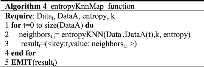
  Every map j will constitute a id-distance vector neighbors_{t, j} of pairs < id,distance > of dimension k for each data sample t in DataA. To do so, Instruction 2 computes for each data sample the entropy distance to its k nearest neighbors. To accelerate the posterior actualization of the nearest neighbors in the reducers, every vector neighbors_{t, j} is sorted in ascending order regarding the distance to the data sample, so that, Dist(neigh₁) < Dist(neigh₂) < …. < Dist(neigh_k).

• (2) Reduce phase: The reduce phase consists of collecting, from the tentative k nearest neighbors provided by the maps, the closest ones for the examples contained in the whole Data. After the map phase, all the elements with the same key have been grouped. A reducer is run over a list (neighbors_{t, 0}, neighbors_{t, 1},.., neighbors_{t, p}) and determines the k nearest neighbors of this data example t.

This function will process every element of such list one after another. Instructions 2 to 6 update a resulting list result with the k neighbors. Since the vectors coming from the maps are ordered according to the distance, the update process becomes faster. This consists of merging two sorted lists up to get k values, so that, the complexity in the worst case is O(k).Therefore, this function compares every distance value of each of the neighbors one by one, starting with the closest neighbor. If the distance is lesser than the current value, the class and the distance of this position is updated with the corresponding values, otherwise we proceed with the following value. Algorithm 5 provides the details of the reduce operation.

In summary, for every instance in the data set, the reduce function will aggregate the values according to function described before. To ease the implementation of this idea, we use the transformation ReduceByKey() from Spark. Algorithm 5 corresponds to the function required in Spark.

4.3 Outlier detection stage

Outlier detection stage can be described as follows: Given a set of N data points or objects and n the expected number of outliers, find the top n objects that are considerably dissimilar from the remaining set of data. Figure 4 presents the flowchart of the outlier detection stage.

Fig. 4

Flowchart of the outlier detection stage

Once it receives all the outputs of the k nearest Neighbors Stage. It is applied one last map function to calculate the outlier degree. Outlier degree is calculated by the sum of k-nearest neighbors. And then considers as outliers are the top n point’s p whose outlier degree is the greatest.

5 General scheme of SEOD

When the size of the dataset is very large, we may exceed the memory allowance of the map tasks. In this case, we also have to split the dataset and carry out the MapReduce process defined above. Algorithm 6 shows the pseudo-code of the whole method with precise details of the functions utilized in Spark. In the following, we describe the most significant instructions, enumerated from 1 to 11

.

As input, we receive the path in the HDFS for dataset as well as the number of maps m and reducers r. We also dispose of the number of neighbors k and the number of outliers n.

Firstly, it creates an RDD object with the dataset formed by m blocks (Line 1). Secondly it performs a parallel operation to normalize the data into the user-defined data structure. Datasets are cached for future reuse (Line 2).Then the map phase divides the DataRDD and counts the data frequency for each split (Line 3). The reduce stage joins all the data frequency and obtains the final data frequency (Line 4). With the data frequency of each attribute among the data set, it calculates attribute entropy (Line 5).

Next, we make use of the mapPartitions() transformation, which runs the KNN function defined in Algorithm 6 on each block of the RDD separately. Instruction 6 broadcasts this attribute entropy into the main memory of all the computing nodes involved. Instruction 7 computes for each data sample the entropy distance to its k nearest neighbors. Instruction 8 consists of collecting, from the tentative k nearest neighbors provided by the maps, the closest ones for the examples contained in the whole Data. In summary, for every instance in the data set, the reduce function will aggregate the values according to function described before. To ease the implementation of this idea, we use the transformation ReduceByKey() from Spark.

After that, it calculates the outlier degree for every data instance, with the resulting neighbors (Line 9).Then it executes a top algorithm to detect outliers (Line 10). Finally, it outputs the outliers (Line 11).

6 Experimental evaluation

6.1 Experimental setup and methodologies

6.1.1 Experimental infrastructure

All experiments are conducted on a Hadoop cluster with one master node and five slave nodes. All the nodes have the following features has 2 Intel Xeon CPU E5-2630 processor, 2 cores per processor, 2.6 GHz and 4 GB of RAM. Nodes are interconnected with 1Gbps Ethernet. Every node runs with ubuntu 14.04 as an operating system and was configured with Hadoop 2.6.5 and Spark 2.0.0. Each node is configured with up to 4 map and 4 reduce tasks running concurrently, sort buffer size set to 1 GB, and replication factor 3.

6.1.2 Datasets

In this experimental study we will use three big data sets. Banana, Penbased and Pokerhand are extracted from the UCI machine learning repository [21].Table 1 summarizes the characteristics of these datasets. We show the number of examples (#Examples), and the number of features (#Features).

Table 1 Summary description of used datasets

6.1.3 Metrics

First, performance evaluation is carried out by the following metrics: precision, recall, F1-measure (Eqs. 4, 5 and 6), where the positive class represents the anomalies and the negative class represents the nominal samples.

$$ precision = \frac{{true\,{\text{positives}}}}{{true\,{\text{positives}} + false\,{\text{positives}}}} $$

(4)

$$ recall = \frac{{true\,{\text{positives}}}}{{true\,{\text{positives}} + false\,{\text{negatives}}}} $$

(5)

$$ F1 = \frac{precision*recall*2}{precision + recall} $$

(6)

Second, we measure the total runtime between launching the program and receiving the results-a common metric for the evaluation of distributed algorithms [13, 22]. The total runtime for the parallel approach includes preprocessing, attribute calculation, calculating k nearest neighbors and top n outlier detection. Third, we measure the speedup. The speedup proves the efficiency of a parallel algorithm comparing against the sequential version of the algorithm. Thus, it measures the relation between the runtime of sequential and parallel versions. In a fully parallel is environment, the maximum theoretical speed up would be the same as the number of used cores [23].

$$ speedup = \frac{base\_line}{parallel\_line} $$

(7)

where base_line is the runtime spent with the sequential version and parallel_time is the total runtime achieved with its improved version.

6.1.4 Algorithms

We compare the proposed methods experimentally. (1) The two step baseline method baseline: first compute the outlier scores of all points utilizing the algorithm in [3] and sort the points based on their outlier scores; (2) EKNN: the state-of-the-art entropy-based outlier detection algorithm EKNN as described in Sect. 1; (3)SEOD: our proposed entropy-based implemented on Spark.

6.1.5 Experimental methodology

We conduct experiments to evaluate the effectiveness of our proposed algorithms using various datasets derived from the Banana, Penbased, and Pokerhand datasets. In all experiments, the same kNN search algorithm is applied to eliminate the influence of the various kNN search algorithms and indexing mechanisms.

6.2 Analysis of results

6.2.1 Evaluation of runtime

Figure 5 shows the mean value of 5 experimental results under different datasets.

Fig. 5

Mean value of the runtime per dataset and algorithm (5 runs)

The Baseline and EKNN outperform the sequential version for every dataset. This Baseline has the best results for the smallest datasets. However, the execution times for larger dataset are still unacceptably long. On the other hand, the performance of the distributed approaches for SEOD is significantly better for larger datasets. Better yet, the larger the dataset, the more SEOD wins. The distribution of the data, and hence the computation, comes with a small network overhead due to serialization, transfer and synchronization. This overhead has a significant impact when the data size is small, and therefore it actually takes more time to distribute the data than directly run the computation. However, this is compensated when the datasets are large enough in terms of instances, which is when the distribution of the data truly makes sense. Now, the bigger the dataset the better runtime achieved. Moreover, it can be seen from Fig. 5 that the runtime of EKNN is higher than Baseline. There is extra attribute calculation of the EKNN.

6.2.2 Evaluation of the effectiveness

In this experiment, we investigate the outlier detection results of the different implementations on the multiple datasets. To measure the performance of the outlier detection algorithms we use the three metrics presented in Sect. 6.1 which show different perspectives of the same results.

Table 2 presents the averaged measures obtained for the different metrics. First, The Entropy-based implementation, namely EKNN and SEOD, presents more competitive results than Baseline in terms of average values. These differences are produced by the K nearest neighbors process of the information entropy. The Entropy-based implementation uses the information of the attributes to find better nearest neighbors, thus leading to a considerable improvement of the detection. Second, The Entropy-based implementations all obtain the same detection results because they use the same entropy distance.

Table 2 Average outlier detection performance on multiple datasets

6.2.3 Evaluation of the influence of parameters

We next evaluate the influence of the number of neighbors k, the number of outliers n and the number of map task m. We use the UCI machine dataset (Table 1).

6.2.4 Influence of varying parameter k

Table 3 presents the results of varying the KNN input parameter k from 10 to 30. The processing time of SEOD increases when k increases. The parameter k determines the number of neighbors, which affects the calculation of outliers. Therefore, too small k cannot completely reflect the neighbor information, and too large k will increase the amount of calculation, so we should choose a suitable k to achieve better detection results.

Table 3 Runtime in seconds of different k

6.2.5 Influence of varying parameter n

Table 4 shows the total runtime when varying the input parameter n, that is, the number of outliers. N is varied from 40 to 120. The processing time of SEOD increases when n increases. The parameter n is closely related to the number of outliers. If the n is too small, all the outliers cannot be selected. If the n is too large, the runtime will increase. Therefore, it is necessary to select an appropriate n according to the user’s needs.

Table 4 Runtime in seconds of different n

6.2.6 Influence of varying parameter m

Table 5 shows the total runtime when varying the input parameter m from 4 to 12. Analyzing Table 5 (line 2–3), For smaller data sets, as m increases, the runtime increases linearly, because for a smaller amount of data, an increase in m leads to a larger communication overhead and a linear increase in time. Analyzing Table 5 (line 4), for the larger dataset, as m increases, the runtime of the SEOD decreases significantly and finally stabilizes. Because the increase of parallelism is beneficial to distributed processing, as the degree of parallelism increases, the efficiency growth will slowly reach a certain saturation point. At this point, the communication time of each node of the cluster is far greater than the calculation time, and the performance of the algorithm tends to gentle or even weak.

Table 5 Runtime in seconds of different m

6.2.7 Evaluation of the scalability

To evaluate the performance of our proposed methods on various dataset sizes, we extract from pokerhand data subsets of different sizes, including Dataset1, Dataset2 and Dataset3. The number of data points gradually grows from one hundred thousand to more than two hundred thousand.

Figure 6 presents the speedup of SEOD using the datasets described above (Table 6) when varying the number of nodes.

Fig. 6

Speedup of SEOD algorithm

Table 6 Summary description of datasets

The speedup of SEOD increases linearly with the number of nodes, and as the data size increases, the speedup performance of the algorithm becomes better and better. Hence, they are limited by the number of cores in the cluster.

Figure 7 presents the runtime of SEOD using the datasets described above (Table 6) when varying the number of nodes.

Fig. 7

Runtime of cluster

According to Fig. 7, the runtime of the SEOD decreases with the increase of the number of working nodes in the cluster, but the downward trend becomes slower. The communication overhead caused by the broadcast of the data in the map phase and the data aggregation in the reduce phase may be the reason. At the same time, it can be seen that the larger the data size, the more obvious the downward trend. The scalability of the proposed model obtains a linear behavior. However, the runtime on dataset3 is pretty high, and reveals a weakness of the proposed algorithm. More hardware will be needed when the runtime matter.

7 Conclusion and future work

Using outlier detection algorithms to extract abnormal phenomena from huge volumes of data is an extremely important yet expensive task. Existing techniques lack proper scaling to large dataset and consider attribute difference. In this paper, we propose the first distributed entropy-based outlier detection approach using the Spark. It is denominated as SEOD. Its main achievement is to handle large-scale datasets with the higher accuracy results than the original k nearest neighbors algorithm. The SEOD first introduces attribute information entropy to distinguish the importance of each attribute. Then, use the weighted Euclidean distance to find the k neighbors of each data instance, and finally use the outlier degree formula to find the outliers. Experiments show that the SEOD has good detection performance, good speedup and scalability, and the ability to process large-scale data sets.

In the SEOD, we only consider the influence of the importance of different attributes on outlier detection, and do not consider the difference of different neighbors, that is, each neighbor is treated equally. However, the difference in k neighbors is also important for outlier degree. As future work, we will study how to treat the information of k neighbors differently in the outlier algorithm under the cloud computing platform.

References

Aggarwal, C.C.: Outlier Analysis. Springer, New York (2015)
Domingues, R., Filippone, M., Michiardi, P., Zouaoui, J.: A comparative evaluation of outlier detection algorithms: experiments and analyses. Pattern Recogn. 74, 406–421 (2017)
Ramaswamy,S., Rastogi, R., Shim, K.: Efficient algorithms for mining outliers from large data sets. In: Paper presented at the ACM SIGMOD International Conference on Management of Data, ACM, pp. 427–438, (2000)
Dean, J., Ghemawat, S.: MapReduce: a flexible data processing tool. Commun. ACM 53(1), 72–77 (2010)
White, T.: Hadoop: The Definitive Guide, 4th edn. O’Reilly, Sebastopol (2015)
Maillo, J., Ramírez, S., Triguero, I., et al.: kNN-IS: an iterative spark-based design of the k-nearest neighbors classifier for big data. Knowl.-Based Syst. 117, 3–15 (2016)
Maillo, J., Luengo, J., García, S., et al.: Exact fuzzy k-nearest neighbor classification for big datasets. In: Paper presented at the IEEE International Conference on Fuzzy Systems, IEEE, (2017)
Zaharia, M., Chowdhury, M., Franklin, M., Shenker, S., Stoica, I.: Spark: cluster computing with working sets. HotCloud 10, 10 (2010)
Zaharia, M., Chowdhury, M., Das, T., Dave, A., Ma, J., McCauley, M., Franklin, M., Shenker, S., Stoica, I.: Resilient distributed datasets: a fault-tolerant abstraction for in-memory cluster computing. In: Paper presented at the Conference on Networked Systems Design and Implementation, pp. 1–14, (2012)
Wu, S., Wang, S.: Information-theoretic outlier detection for large-scale categorical data. IEEE Trans. Knowl. Data Eng. 25, 589–602 (2013)
Subramanyam, R.B.V., Sonam, G.: Map-reduce algorithm for mining outliers in the large data sets using twister programing model. Int. J. Comput. Sci. Electron. Eng. 3(1), 81–86 (2015)
Guo, Y.P., Liang, J.Y., Zhao, X.W.: An outlier detection algorithm for mixed data based on MapReduce. J. Chin. Comput. Syst. 35(9), 1961–1966 (2014)
Cao, L., Yan, Y., Kuhlman, C., et al.: Multi-tactic distance-based outlier detection. In: Paper presented at the IEEE International Conference on Data Engineering, IEEE, pp. 959–970, (2017)
Hu, C.P., Qin, X.L.: A density-based local outlier detecting algorithm. J. Comput. Res. Dev. 47(12), 2110–2116 (2010)
Wang, J.H., Zhao, X.X., Zhang, G.Y.: NLOF: a new density-based local outlier detecting algorithm. Comput. Sci. 40(8), 181–185 (2013)
Xin, L.L., He, W., Yu, J.: An outlier detection algorithm based on density difference. J. Shangdong Univ. (Eng. Sci.) 45(3), 7–14 (2015)
Shannon, C.: A mathematical theory of communication. Bell Syst. Tech. J. 27(379–423), 623–656 (1948)
Filippone, M., Sanguinetti, G.: Information theoretic novelty detection. Pattern Recogn. 43(3), 805–814 (2010)
Jiang, F., Sui, Y., Cao, C.: An information entropy-based approach to outlier detection in rough sets. Expert Syst. Appl. 37(9), 6338–6344 (2010)
Pang, G., Cao, L., Chen, L., et al.: Unsupervised feature selection for outlier detection by modelling hierarchical value-feature couplings. In: Paper presented at the International Conference on Data Mining, IEEE, pp. 410–419, (2017)
Asuncion A.: UCI machine learning repository, (2013)
Yan, Y., Cao, L., Kulhman, C., et al: Distributed local outlier detection in big data. In: Paper presented at The ACM SIGKDD International Conference, pp. 1225–1234, (2017)
Sarumiab, O.A., Leungb, C.K., Adetunmbi, A.O.: Spark-based data analytics of sequence motifs in large omics data. Procedia Computer Science 136, 596–605 (2018)
Acknowledgements
This work was supported by the Civil Aviation Flight Data Analysis under No. XM2852 and Key Scientific and Technological Research Projects in Henan Province (Grand No. 192102210125).
Author information
Authors and Affiliations
Corresponding author
Additional information
Publisher's Note
Springer Nature remains neutral with regard to jurisdictional claims in published maps and institutional affiliations.
Rights and permissions
About this article
Cite this article
Feng, G., Li, Z., Zhou, W. et al. Entropy-based outlier detection using spark. Cluster Comput 23, 409–419 (2020). https://doi.org/10.1007/s10586-019-02932-2
Received:
Revised:
Accepted:
Published:
Issue Date:
DOI: https://doi.org/10.1007/s10586-019-02932-2