Cosmological models in Sáez-Ballester theory with bilinear varying deceleration parameter

Abstract

The basic purpose of this communication, is to investigate the dynamical nature of Bianchi type-I universe with perfect fluid content in Sáez-Ballester (SB) theory (Phys. Lett. A 113:467–470, 1986). We got the solution of modified Einstein’s field equations (EFEs) by considering the bilinearly varying deceleration parameter (BVDP) and the gravitational constant $(G)$ as a power function of average scale factor $a(t)$. We assumed that BVDP is function of cosmic time with $q(t)=\frac{\alpha (1-t)}{1+t}$, $\alpha \geq 0$. Our finding suggests that present universe has had transitional phase of expansion which was decelerating in the past and is accelerating phase at present time. We also observed that the DE parameter $(\Lambda )$ and energy density parameter $(\rho )$ are decreasing with respect to cosmic time and converge to a very small value at the late time. This result is in strong agreement with recent observations. Physical and geometric properties of the cosmological parameters are also presented in the communication.

1 Introduction

In recent observations of the SNe Ia supernovae (Riess et al. (1998), Perlmutter et al. (1998, 1999)) and the power spectrum fluctuation in the cosmic radiation indicate evidences regarding the presence of mysterious dark energy (DE) in the universe. (Spergel et al. (2003)). We know that DE models of the universe have significant role in theoretical study of structure of the universe. The DE is assumed as the best candidate to explain present cosmic acceleration. It is also believed that $96\%$ of the universe consists of DE and dark matter. The DE is usually characterized by equation of state parameter (EoS) and is defined as $\omega =\frac{p}{\rho }$, here $\omega$ is EoS parameter, $p$ is the fluid pressure and $\rho$ is energy density of the universe. Both the observations i.e. cosmic microwave background radiation (CMBR) and SNe Ia suggest to further study regarding acceleration and expanding models of the universe with $\Omega _{m}$ and $\Omega _{\Lambda }$, here $\Omega _{m}$ represent the DM density parameter and $\Omega _{\Lambda }$ represent DE density parameter and also values of $\Omega _{m} \approx 0.3$ and $\Omega _{\Lambda }\approx 0.7$. During literature survey it has been noticed that cosmological constant problem always much debatable among researchers/cosmologist since its inception (Weinberg (1989), Padmanabhan (2003)). Also, the DE density parameter $\Omega _{\Lambda }$ corresponds to cosmological constant $\Lambda$ is a very small non-negative quantity at present time. Therefore, we are interested to investigate the dependence of $\Lambda$ upon scale factor $(a(t))$ at certain level of accuracy.

In physical cosmology the deceleration parameter (DP) is the key parameter to categorized the different evolution epochs of the universe. The changes in sign of the value of DP from positive ($q>0$) to negative ($q<0$) indicate phase transition in the evolution of the universe. As discussed above Riess et al. (1998) and Perlmutter et al. (1998) have established that present value of DP is negative for observed red-shifted magnitude of supernova SNe Ia observations. In 1998, Perlmutter et al. (1998) and Riess et al. (2001), Caldwell and Doran (2004) have also found that the value of DP lies in range $-1\leq q_{0}\leq 0$. On the basis of observational values of DP they reached at the conclusion that the present universe is an undergoing accelerating phase of expansion. In continuation to this Schuecker et al. (1998) also observed that present value of $q_{0}$ varies between −1.27 and 2.

Along with time-varying DP we are also familiar with the importance of Hubble parameter $H$. As the sign of $H$ and $q$ indicate the expansionary nature of the universe either increasing up or slowing down with time. Hence, sign of $H$ and $q$ classify expansionary nature of the universe as: if $H>0$, $q<0$, then universe is an expanding with accelerating rate; if $H>0$, $q=0$, then rate of expansion is constant; if $H>0$, $q>0$, then rate of expansion is decreasing with cosmic time (Bolotin et al. (2015)).

After the discovery of accelerating and expanding many authors tried to find the rate of universe expansion and constructed models with time varying DP. Mak and Harko (2002) had generated solution of gravitational field equations with time varying DP i.e. $q(t)$ and established that DP is not a constant quantity. In the similar context, several researcher including Our peer group have constructed several cosmological models with time varying DP and published fruitful results (Akarsu and Dereli (2012), Amirhashchi and Pradhan (2011), Reddy et al. (2013), Mishra et al. (2012), Mishra and Chand (2016, 2017), Chand et al. (2016) and Chawla et al. (2014). Further, Akarsu and Dereli (2012) have proposed DP as a linear function of cosmic time $t$ as $q=-kt+m-1$, here $k$ and $m$ are non negative constants. In this context our peer research group Mishra et al. have investigated few cosmological models with time-dependent DP along with proper anastz $q(t)=n. sech^{2}(\alpha t))-1$ and $q(t)=-1+\frac{n\alpha }{(t+\alpha )^{2}}$ and published fruitful results. In 2016, we proposed DP as bilinear function of cosmic time along with $q(t)=\frac{\alpha (1-t)}{1+t}$, here $\alpha$ is a non negative constant (Mishra and Chand 2016).

The general theory of relativity (GTR) is the best suited theory to describe the universe and $\Lambda$ cold dark matter model ($\Lambda$CDM) is the most natural model of the universe, but the early time inflationary and late time accelerating expansionary nature of the universe has not properly addressed by GTR. Therefore, to resolve this issue there is need either modify the GTR or develop a new theory, which will gives the complete description of the universe. During the literature survey has been noticed a large number of alternative theories of gravity were proposed by cosmologists. Among these alternative theories the scalar-tensor theories is interesting and beneficial for such study.

In 1986, Sáez and Ballester (1986) proposed a scalar-tensor theory of gravity, known as Sáez Ballester theory. In this theory the metric is coupled with a dimensionless scalar field in a different way. This coupling provide a reasonable description of the weak field in which an accelerated expansion regime reflect further. The action for the SB theory can be expressed as,

$$ A=\int _{\mathbb{R}} (L+\chi L_{m})\sqrt{-g}dx^{1}dx^{2}dx^{3}dx^{4}, $$

(1)

with a slight variation of the metric and scalar field vanishing at the boundary of region ℝ, the variation principle leads the fields equations

$$ G_{ij}-w \phi ^{r}(\phi _{,i}\phi _{,j}-\frac{1}{2}g_{ij}\phi _{,k} \phi ^{,k}) =8\pi T_{ij}, $$

(2)

where $L_{m}$ is the matter Lagrangian, $g=|g_{ij}|$, $G_{ik}=R_{ik}-\frac{1}{2}Rg_{ik}$ is the Einstein tensor, ℝ is an arbitrary region of integration, $x^{i}$ are the coordinates, $T_{ij}$ is the energy momentum tensor, $w$ is a dimensionless constant, $\phi$ is the scalar field and $r$ is an arbitrary constant. The scalar field $\phi$ satisfying the following equations;

$$ 2\phi ^{r}\phi ^{,k}_{;k}+r\phi ^{r-1}\phi _{,k}\phi ^{,k}=0. $$

(3)

Numerous modification of GTR is accepted the theory of variable gravitation constant $G$, based on different arguments proposed by several authors Dirac (1974), Wesson (1980), Canuto and Narlikar (1980), Arbab (1997) and agreed that $G$ varying cosmology is consistent with cosmological observations. In recent past several authors Ramesh and Umadevi (2016), Rasouli and Moniz (2018), Rao et al. (2018), Sharma et al. (2019) and investigated cosmological models in the context of SB theory. Recently, our peer group Mishra and Chawla et al. (2014) and Mishra and Dua (2019) have already published the detail study of cosmological models with time varying parameters DP. gravitational constant $(G)$ and cosmological constant $(\Lambda )$ in SB theory. Very recently, Rasouli et al. (2020), have published their work entitled ‘Late time cosmic acceleration in modified Sáez and Ballester theory’, under this work they have discussed two scalar field, one associated with SB theory and other with extra dimension. Really, this provide the scope of the induced matter theory. Such study also indicate the close resemblance with standard SB theory as well as alternative theory to GTR. It is also submitted that the Bianchi Type-I models are the simplest models which are spatial homogeneous and anisotropic and whose spatial sections are flat but the expansion or contraction rate is direction-dependent. Therefore, in the present communication, we have investigated the Bianchi type-I space-time universe model with time-dependent BVDP with relation $q(t)=\frac{\alpha (1-t)}{1+t}$, along with time-variable cosmological constant $(\Lambda )$ in the frame work of scalar-tensor SB theory.

The outline of the paper is as follows: In Sect. 2, we presented mathematical equations governing the model. Solutions of field equations presented in Sect. 3. Section 4, physical and geometric properties of cosmological parameter have been discussed. Section 5, contains results and discussions of the study. Finally, concluding remarks of the study have been summarized in Sect. 6.

2 Mathematical equations governing the model

To present this study in more effective ways we considered a spatially homogeneous and an anisotropic Bianchi type-I space-time universe expressed by the metric given below:

$$ ds^{2} = - dt^{2} + R_{1}^{2}(t)dx^{2}+R_{2}^{2}(t)dy^{2}+R_{3}^{2}(t)dz^{2}, $$

(4)

where $R_{1}$, $R_{2}$ and $R_{3}$ are potential functions. From review of the literature, it is observed that modified EFEs in SB theory as given by Sáez and Ballester (1986), may be expressed as:

$$ G_{ik}-\omega \phi ^{r}\Biggl(\phi _{,i}\phi _{,k}-\frac{1}{2}g_{ik} \phi _{,j}\phi ^{,j}\Biggr) =-8\pi G(t)T_{ik}+\Lambda (t)g_{ik} $$

(5)

where, $G_{ik}=R_{ik}-\frac{1}{2}Rg_{ik}$ is the Einstein tensor, $T_{ik}$ is the energy momentum tensor, $\omega$ is a dimensionless constant, $\phi$ is the scalar field and $r$ is an arbitrary constant. Further the scalar field $(\phi )$ may satisfy the following conditions:

$$ 2\phi ^{r}\phi ^{,j}_{;j}+r\phi ^{r-1}\phi _{,k}\phi ^{,k}=0, $$

(6)

here commas and semi-colon denote partial and co-variant derivatives, respectively. The expression for energy-momentum tensor $(T_{ik})$ in case of perfect fluid distribution may be expressed as:

$$ T_{ik}=(\rho +p)u_{i}u_{k}+pg_{ik}, $$

(7)

here $\rho$ and $p$ are the energy density and pressure for cosmic fluid. Further, $u^{i}=(0,0,0,1)$ is the four velocity vector with $g_{ik}u^{i}u^{k}=-1$. As presented above now the modified EFEs (5), scalar field equation (6) and energy conservation equation, i.e.

$$ T_{;k}^{ik}=0, $$

(8)

leads to the following set of field equations as:

$$\begin{aligned}& \frac{\ddot{R_{1}}}{R_{1}}+\frac{\ddot{R_{2}}}{R_{2}}+ \frac{\dot{R_{1}}\dot{R_{2}}}{R_{1} R_{2}}-\frac{1}{2}\omega \phi ^{r} \dot{\phi }^{2} =-8\pi G p+\Lambda , \end{aligned}$$

(9)

$$\begin{aligned}& \frac{\ddot{R_{2}}}{R_{2}}+\frac{\ddot{R_{3}}}{R_{3}}+ \frac{\dot{R_{2}}\dot{R_{3}}}{R_{2}R_{3}}-\frac{1}{2}\omega \phi ^{r} \dot{\phi }^{2} =-8\pi G p+\Lambda , \end{aligned}$$

(10)

$$\begin{aligned}& \frac{\ddot{R_{3}}}{R_{3}}+\frac{\ddot{R_{1}}}{R_{1}}+ \frac{\dot{R_{3}}\dot{R_{1}}}{R_{3}R_{1}}-\frac{1}{2}\omega \phi ^{r} \dot{\phi }^{2} =-8\pi G p+\Lambda , \end{aligned}$$

(11)

$$\begin{aligned}& \frac{\dot{R_{1}}\dot{R_{2}}}{R_{1}R_{2}}+ \frac{\dot{R_{2}}\dot{R_{3}}}{R_{2}R_{3}}+ \frac{\dot{R_{3}}\dot{R_{1}}}{R_{3}R_{1}} +\frac{1}{2}\omega \phi ^{r} \dot{\phi }^{2} =8\pi G \rho +\Lambda , \end{aligned}$$

(12)

$$\begin{aligned}& \ddot{\phi }+\dot{\phi }\Biggl(\frac{\dot{R_{1}}}{R_{1}}+ \frac{\dot{R_{2}}}{R_{2}}+\frac{\dot{R_{3}}}{R_{3}}\Biggr) + \frac{r\dot{\phi }^{2}}{2\phi }=0, \end{aligned}$$

(13)

$$\begin{aligned}& \dot{\rho }+3(\rho +p)H=0, \end{aligned}$$

(14)

As we know that in the above equations $\Lambda$ describe the vacuum energy density with energy density $\rho _{\Lambda }$ and pressure $p_{\Lambda }$ satisfying the equation of state $p_{\Lambda }=-\rho _{\Lambda }$. Moreover, the vanishing divergence of Einstein tensor $G_{ij}$ leads to

$$ 8\pi G\{\dot{\rho }+3(\rho +p)H\}+8\pi \dot{G}\rho + \dot{\Lambda }=0. $$

(15)

Equation (15) with the help of equation (14), yields the coupling between $G$ and $\Lambda$ may be expressed as:

$$ 8\pi \dot{G}\rho + \dot{\Lambda }=0. $$

(16)

To move this study further we are required the solution of above stated field equations (9) to (14), which is being presented in Sect. 3.

3 Solution of the field equations

As the field equations (9) to (14) is the set of five non-linear differential equations containing eight unknown parameters, viz. $R_{1}, R_{2}, R_{3}, p, \rho , \Lambda , G$ and $\rho$. For an explicit solution of the equations more constraints/equations required. For the same purpose here we may consider following physically plausible relations:

i) Analysis with time-dependent DP

As dynamics of the universe is described by time-dependent cosmic scale factor $a(t)$. The time dependence of $a(t)$ reflects various significant events in evolution history of the universe. Therefore, to study the dynamic history of the universe with time we are needing more dynamical & kinematical parameters related to scale factor and its derivative. To apply this we may expand the scale factor $a(t)$ with the help of Taylor’s series as discussed below:

$$\begin{aligned}& a(t)= a(t_{0})+\dot{a}(t_{0})(t-t_{0})+\frac{1}{2}\ddot{a}(t_{0})(t-t_{0})^{2}+\cdots, \end{aligned}$$

(17)

$$\begin{aligned}& a(t)= a(t_{0})[1+H_{0}(t)(t-t_{0})-\frac{q_{0}H_{0}^{2}}{2}(t-t_{0})^{2}+\cdots.]. \end{aligned}$$

(18)

The second and third term of the above expansion suggest the Hubble’s parameter (H) and the DP (q), two measurable parameters in Cosmology. The present value of $H_{0}$ and $q_{0}$ may be defined as

$$\begin{aligned}& H_{0}(t)=\frac{\dot{a}(t_{0})}{a(t_{)})}, \end{aligned}$$

(19)

$$\begin{aligned}& q_{0}(t)=-\frac{a(t_{0})\ddot{a}(t_{0})}{\dot{a}(t_{0})}, \end{aligned}$$

(20)

The redshift parameter $z$ in term of average scale factor $a(t)$ may be written as

$$ z(t)= H_{0}(t)(t-t_{0})-\frac{q_{0}H_{0}^{2}}{2}(t-t_{0})^{2}+\cdots, $$

(21)

here, lower script ‘0’ denote present value of the parameter. The Hubble’s parameter determines the rate of expansion of universe, while that the DP determines the rate at which expansion is slowing down or speeding up. The Planck collaboration 2015 (Ade et al. (2016)) suggested that $H_{0}=67.8\pm .9~\mbox{Km}\,\mbox{s}^{-1}\,\mbox{Mpc}^{-1}$. The positive sign of DP $(q>0)$ correspond to decelerating universe whereas negative sign of DP $(q<0)$ indicates accelerating universe. In 1998, Berman (1998) had investigated models with constant DP whereas Mishra et al. (2012) suggested a time-dependent DP as

$$\begin{aligned}& a(t)= sinh(\alpha t)]^{\frac{1}{n}}, \end{aligned}$$

(22)

$$\begin{aligned}& q(t)= n.sech^{2}(\alpha t)-1, \end{aligned}$$

(23)

where $n$ & $\alpha$ are non negative constants.

Our peer group also derived cosmological models by considering $q$ as function of time as

$$\begin{aligned}& a(t)= [t^{\alpha }e^{t}]^{\frac{1}{n}}, \end{aligned}$$

(24)

$$\begin{aligned}& q(t)= -1+ \frac{n\alpha }{(\alpha +t)^{2}}, \end{aligned}$$

(25)

and published fruitful results (Mishra and Chand (2016, 2017)). During investigation of literature it has been noticed that Akarsu and Dereli (2012) had proposed DP as a linear function of cosmic time and termed as linearly varying law for deceleration parameter (LVDP) and given by equation

$$ q(t)=-kt + m-1, $$

(26)

here $k$ is a positive constant with the dimension of inverse of time and $m>1$ is a dimension free constant.

Motivated from above mentioned study we wish to investigate the dynamic nature of the universe by assuming DP $(q)$ as a bilinear function of cosmic time ‘t’ with specific assumption as proposed by Mishra and Chand (2016) as:

$$ q(t)=\frac{\alpha (1-t)}{1+t}, $$

(27)

The expressions for $H(t)$ and $a(t)$ are given by

$$\begin{aligned}& H(t)=\frac{1}{(1-\alpha )t+2\alpha \log (1+t)}, \end{aligned}$$

(28)

$$\begin{aligned}& a(t)=a_{0} t^{\frac{1}{1+\alpha }}.e^{F_{1}(t)} \end{aligned}$$

(29)

where

$$\begin{aligned} F_{1}(t)={}& \frac{\alpha }{(1+\alpha )^{2}} t+ \frac{-2\alpha +\alpha ^{2} }{6(1+\alpha )^{3}}t^{2}+ \frac{3\alpha -2\alpha ^{2}+\alpha ^{3}}{18(1+\alpha )^{4}}t^{3}\\&{}+ \frac{-18\alpha +11\alpha ^{2}-14\alpha ^{3}+2\alpha ^{4}}{180(1+\alpha )^{5}}t^{4}+ O(t^{5}). \end{aligned}$$

From equations (27)–(29), it is analyzed following possibilities for presented models as:

• i) $0<\alpha <1$, $0< t<1$, then $q>0$, $H>0$, $a>0$

• ii) $0<\alpha <1$, $t>1$, then $q<0$, $H>0$, $a>0$

For better understanding and validation of the proposed model we have presented variation of some cosmological parameters with cosmic time in Figs. 1 to 8. The variation of Hubble parameter with time for $n=0.5, 1.0, 1.5$ and 2.0 is presented in Fig. 1. It is observed that $H$ is decreasing with cosmic time and further it approaches to a small value at the late time. Figure 2 depicts the variation of $q$ with time. It is also clear from Fig. 2 that the universe shows deceleration phase for; $0< t<1$, $\alpha >0$. Constant expansion for; $t=0$, Exponential expansion phase for; $t>1$, $0<\alpha <1$. Super exponential expansion phase for; $t>1, \alpha >1$. This suggest that the universe is decelerating in past and accelerating at present time, hence DP must show signature flipping (Padmanabhan (2002, 2003), Amendola (2003)). Therefore, our universe has transitional phase, which is validated with recent SNe Ia supernova observations.

Fig. 1

Plot of Hubble’s parameter $H$ versus time $t$

Fig. 2

Plot of DP $q$ versus time $t$

ii) Analysis with power law

A set of non-linear differential equations is always difficult to solve, so to remove this complication we may assume the power law relation between $G$ and $a(t)$ as suggested by Luis (1985), Johri and Kalyani (1994) as

$$ 8\pi G= G_{0}[a(t)]^{n}, $$

(30)

where, $G_{0}$ is proportionality constant and $n$ is ordinary positive constant, we have written $8\pi G$ instead of $G$ for mathematical convenience. On simplification of field equations (11)-(16), we have the following mathematical expression,

$$\begin{aligned}& \frac{R_{1}}{R_{2}}=k_{1}e^{l_{1} \int a^{-3}dt }, \end{aligned}$$

(31)

$$\begin{aligned}& \frac{R_{2}}{R_{3}}=k_{2}e^{l_{2} \int a^{-3}dt }, \end{aligned}$$

(32)

$$\begin{aligned}& \frac{R_{1}}{R_{3}}=k_{3}e^{l_{3} \int a^{-3}dt }, \end{aligned}$$

(33)

here $k_{1},k_{2},k_{3},l_{1},l_{2},l_{3}$ are the constant of integration.

After the solving above equations (31)-(33), we have expression for metric potential function $R_{1}(t)$, $R_{2}(t)$, $R_{3}(t)$ as

$$\begin{aligned}& R_{1}(t)= a_{1} t^{\frac{1}{1+\alpha }}.exp{\{F_{1}(t)+m_{1} F_{2}(t) \}}, \end{aligned}$$

(34)

$$\begin{aligned}& R_{2}(t)= a_{2} t^{\frac{1}{1+\alpha }}.exp{\{F_{1}(t)+m_{2} F_{2}(t) \}}, \end{aligned}$$

(35)

$$\begin{aligned}& R_{3}(t)= a_{3} t^{\frac{1}{1+\alpha }}.exp{\{F_{1}(t)+m_{3} F_{2}(t) \}}, \end{aligned}$$

(36)

here

$F_{2}(t)=\int {t^{\frac{-3}{1+\alpha }}.e^{-3F(t)}}dt$, $a_{1}=(k_{1}k_{3})^{\frac{1}{3}}$, $a_{2}=(k_{1}^{-1}k_{2})^{\frac{1}{3}}$, $a_{3}=(k_{2}k_{3})^{\frac{-1}{3}}$, $m_{1}=\frac{l_{1}+l_{3}}{3}$, $m_{2}=\frac{l_{2}-l_{1}}{3}$, $m_{3}=- \frac{l_{2}+l_{3}}{3}$.

On integrating equation (13) twice and using equation (28), we have expression for scalar field $\phi$ as

$$ \phi (t)=\Biggl[\frac{2+r}{2}\{\phi _{0} F_{2}(t)+\phi _{1}\}\Biggr]^{ \frac{2}{2+r}}. $$

(37)

The metric equation (4) can be written as after substituting the values of $A$, $B$ and $C$ from equations (34)-(36),

$$\begin{aligned} ds^{2} =& -dt^{2} + t^{\frac{2}{1+\alpha }}.e^{2F_{1}(t)}[a_{1}^{2}e^{2m_{1} F_{2}(t)}dx^{2} \\ &{} +a_{2}^{2}e^{2m_{2} F_{2}(t)}dy^{2}+a_{3}^{2}e^{2m_{3} F_{2}(t)}dz^{2}]. \end{aligned}$$

(38)

4 Physical and geometric behavior of the proposed model

To discuss the physical and geometric nature of the model, we obtained the below mention equation by using equations (9) and (12)

$$ 8\pi G(\rho +p)=\frac{\dot{R_{2}}\dot{R_{3}}}{R_{2}R_{3}}+ \frac{\dot{R_{3}}\dot{R_{1}}}{R_{3}R_{1}}-\frac{\ddot{R_{1}}}{R_{1}} - \frac{\ddot{R_{2}}}{R_{2}}+\omega \phi ^{r}\dot{\phi }^{2}, $$

(39)

For further simplification it is assumed that fluid obeys the equation of state of the form $p=\gamma \rho$, here $0\leq \gamma \leq 1$. The value of $\gamma$ classify the universe model as a matter-dominated universe model $(\gamma =0)$, radiation dominated universe model $(\gamma =\frac{1}{3})$ and Zel’dovich fluid or stiff fluid universe model $(\gamma =1)$. On using these relations in equation (39), we obtained following set of equations:

$$ \rho =\frac{1}{8\pi G(1+\gamma )}\Biggl[ \frac{\dot{R_{2}}\dot{R_{3}}}{R_{2}R_{3}}+ \frac{\dot{R_{3}}\dot{R_{1}}}{R_{3}R_{1}} -\frac{\ddot{R_{1}}}{R_{1}} - \frac{\ddot{R_{2}}}{R_{2}}+\omega \phi ^{r}\dot{\phi }^{2}\Biggr], $$

(40)

&

$$\begin{aligned} \rho =&\frac{1}{8\pi (1+\gamma )G_{0} T^{n}}\Biggl[ \frac{(m_{1}+m_{2})m_{3}-(m_{1}^{2}+m_{2}^{2})+\omega \phi _{0}}{T^{6}} \\ &{}- \frac{2[1+\alpha +(1-\alpha )t]}{(1+t)[(1-\alpha )t+2\alpha \log (1+t)]^{2}} \Biggr], \end{aligned}$$

(41)

On simplification of equations (12) and (40), the expression for DE candidate $\Lambda$ is given by:

$$\begin{aligned}& (1+\gamma )\Lambda = \frac{\ddot{R_{1}}}{R_{1}} + \frac{\ddot{R_{2}}}{R_{2}}+(1+\gamma ) \frac{\dot{R_{1}}\dot{R_{2}}}{R_{1}R_{2}}+\gamma \frac{\dot{R_{2}}\dot{R_{3}}}{R_{2}R_{3}} \\& \phantom{(1+\gamma )\Lambda =\,\,}{}+\gamma \frac{\dot{R_{3}}\dot{R_{1}}}{R_{3}R_{1}} +\frac{\gamma -1}{2}\omega \phi ^{r}\dot{\phi }^{2}, \end{aligned}$$

(42)

$$\begin{aligned}& \Lambda = \frac{1}{1+\gamma }\Biggl[ \frac{5+2\alpha +3\gamma +(4-\alpha +3\gamma )t}{(1+t)[(1-\alpha )t+2\alpha \log (1+t)]^{2}} \\& \phantom{\Lambda \, }{}+ \frac{(\gamma -1)\omega \phi _{0}+(2-\gamma )(m_{1}^{2}+m_{2}^{2})-\gamma m_{3}+2m_{1}m_{2}}{2T^{6}}\! \Biggr], \end{aligned}$$

(43)

where $T=t^{\frac{1}{1+\alpha }}e^{F_{1}(t)}$. In literature it is also assumed that the coefficient of shear viscosity is proportional to scalar expansion i.e. $\eta \propto \theta$, which leads to the equation,

$$ \eta = \eta _{0} \theta , $$

(44)

here $\eta _{0}$ is proportionally constant, $\theta = 3H$. Since the relation (44) is already discussed in the literature so we have assumed $p= \gamma \rho$ and obtained following equation;

$$\begin{aligned} p =&\frac{\gamma }{8\pi (1+\gamma )G_{0} T^{n}}\Biggl[ \frac{(m_{1}+m_{2})m_{3}-(m_{1}^{2}+m_{2}^{2})+\omega \phi _{0}}{T^{6}} \\ &{}- \frac{2[1+\alpha +(1-\alpha )t]}{(1+t)[(1-\alpha )t+2\alpha \log (1+t)]^{2}} \Biggr]. \end{aligned}$$

(45)

The expressions for vacuum energy density $(\rho _{\Lambda }=-\frac{\Lambda }{8\pi G})$, critical density $(\rho _{c}=\frac{3H^{2}}{8\pi G})$, dark matter density parameter $(\Omega _{m}=\frac{\rho }{\rho _{c}})$ and dark energy density parameter $( \Omega _{\Lambda }=\frac{\rho _{\Lambda }}{\rho _{c}})$ are given as

$$\begin{aligned}& \rho _{\Lambda }=\frac{-1}{G_{0}(1+\gamma )T^{n}}\Biggl[ \frac{5+2\alpha +3\gamma +(4-\alpha +3\gamma )t}{(1+t)[(1-\alpha )t+2\alpha \log (1+t)]^{2}}, \\& \quad {}+ \frac{(\gamma -1)\omega \phi _{0}+(2-\gamma )(m_{1}^{2}+m_{2}^{2})-\gamma m_{3}+2m_{1}m_{2}}{2T^{6}} \Biggr], \end{aligned}$$

(46)

$$\begin{aligned}& \rho _{c}=\frac{3}{G_{0}\{(1-\alpha )t+2\alpha \log (1+t)\}^{2}T^{n}}, \end{aligned}$$

(47)

$$\begin{aligned}& \Omega _{m}= \frac{\{(1-\alpha )+2\alpha \log (1+t)\}^{2}}{24\pi (1+\gamma )} \\& \quad \quad {} \times \Biggl[\{(m_{1}m_{3}-m_{1}^{2} +m_{2}m_{3}-m_{2}^{2}+\omega \phi _{0})\div {T^{6}}\} \\& \quad \quad {}-\{(2+2\alpha +t-\alpha t)\div ((1+t)(1-\alpha )t \\& \quad \quad {}+2\alpha \log (1+t))^{2} \}\Biggr], \end{aligned}$$

(48)

$$\begin{aligned}& \Omega _{\Lambda }= \frac{-\{(1-\alpha )+2\alpha \log (1+t)\}^{2}}{3(1+\gamma )} \\& \quad \quad {}\times \Biggl[ \frac{(\gamma -1)\omega \phi _{0}}{2T^{6}}+ \frac{5+2\alpha +3\gamma +(4-\alpha +3\gamma )t}{(1+t)[(1-\alpha )t+2\alpha \log (1+t)]^{2}} \\& \quad \quad {}+ \frac{(2-\gamma )(m_{1}^{2}+m_{2}^{2})-\gamma m_{3}+2m_{1}m_{2}}{T^{6}} \Biggr]. \end{aligned}$$

(49)

Total density parameter of the universe is $\Omega _{Total}=\Omega _{m}+\Omega _{\Lambda }$.

Expressions for physical quantities such as spatial volume $(V)$, expansion scalar $(\theta )$, directional Hubble’s parameters $(H_{i})$, anisotropy parameter $(A_{m})$ and shear scalar $(\sigma )$ are presented as follow:

$$\begin{aligned}& V(t)= a_{0}^{3}t^{\frac{3}{1+\alpha }}e^{3F_{1}(t)}, \end{aligned}$$

(50)

$$\begin{aligned}& \theta (t)=\frac{3}{(1-\alpha )t+2\alpha \log (1+t)}, \end{aligned}$$

(51)

$$\begin{aligned}& H_{i}(t)= \frac{(1-\alpha )m_{i}+2\alpha \log (1+t)+t^{\frac{3}{1+\alpha }}e^{3F_{1}(t)}}{[(1-\alpha )t+2\alpha \log (1+t)]t^{\frac{3}{1+\alpha }}e^{3F_{1}(t)}} ; \\& \quad i=1,2,3 \end{aligned}$$

(52)

$$\begin{aligned}& A_{m}(t)= \frac{M}{3t^{\frac{6}{1+\alpha }}e^{6F_{1}(t)}[(1-\alpha )t+2\alpha \log (1+t)]^{2}}, \end{aligned}$$

(53)

$$\begin{aligned}& \sigma ^{2}(t)=\frac{1}{2}\Bigl\{ \Bigl(\frac{\dot{R_{1}}}{R_{1}} \Bigl)^{2}+\Bigl(\frac{\dot{R_{2}}}{R_{2}}\Bigl)^{2}+\Bigl( \frac{\dot{R_{3}}}{R_{3}}\Bigl)^{2}\Bigr\} -\frac{\theta ^{2}}{3}= \frac{M}{t^{\frac{6}{1+\alpha }}e^{6F_{1}(t)}}, \end{aligned}$$

(54)

here, $M=m_{1}m_{2}+m_{2}m_{3}+m_{3}m_{1}=-\frac{1}{2}(m_{1}^{2}+m_{2}^{2}+m_{3}^{2})$.

$$ \frac{\sigma ^{2}}{\theta ^{2}}= \frac{M^{2}[(1-\alpha )t+2\alpha \log (1+t)]^{2}}{3t^{\frac{6}{1+\alpha }}e^{6F_{1}(t)}}, $$

(55)

It is observed from equation (50) that spatial volume $V(t)$ is zero at $t=0$ and after that it is exponentially increasing with cosmic time. Equation (51) shows the expansion scalar $\theta (t)$ is infinite at the beginning i.e. $t=0$. It suggest that universe starts evolving with zero volume and infinite expansion rate at $t=0$, which is Big-Bang scenario. As $t\rightarrow \infty$, volume become infinity where $H$, $\theta$$\sigma$, $A_{m}$ approaches to zero. Also $\frac{\sigma ^{2}}{\theta ^{2}}$ is approaches to zero as $t\rightarrow \infty$, therefore, universe approaches to isotropy at late time. For better understanding of the model we have presented graphical representation of calculated parameters, we use the following values for constants $\alpha =0.5$, $1.0, 1.5, \gamma = 0$, $1/3,1, n=2$, $\phi _{0}=G_{0}= \omega =1$, $m_{1}=m_{2}=m_{3}=-1$.

Stability analysis

As already discussed in Sect. 1 that the universe is undergoing in an accelerating expansion phase at present epoch and it is also believed that a mysterious force (DE) may be responsible for this accelerating expansion. But unfortunately, there is not enough information about DE till date. Therefore, it is necessary to know various aspects of DE and its relevance with different kinds of cosmological models. In literature it has been realize that various forms of DE like quintessence, chaplygin gas, k-essence, braneworld models (Ratra and Peebles (1998), Kamenshchik et al. (2001), Armendariz-Picon et al. (2000), Dvali et al. (2000)) have been proposed by cosmologists. These forms give different families of curves of scale factor a(t). To categorize the various forms of DE Sahni et al. (2003) have been proposed a diagnostic pair, known as ‘statefinder diagnostic’ and is defined using the second and third order derivatives of the scale factor a(t). We have obtained expressions for statefinder diagnostic pair $(r,s)$ for presented model as

$$\begin{aligned}& r(t)= \\& \quad \frac{\alpha [1+2\alpha +4\alpha \log (1+t)+(2-6\alpha )t+(-1+2\alpha )t^{2}]}{(1+t)^{2}}, \end{aligned}$$

(56)

$$\begin{aligned}& s(t)=2[-1+\alpha +2\alpha ^{2}-2(-1+\alpha +3\alpha ^{2})t \\& \quad \quad {}-(1+\alpha -2 \alpha ^{2})t^{2} +4\alpha ^{2}\log (1+t)]\div 3[2\alpha -1 \\& \quad \quad {}-(2\alpha +1)t](1+t), \end{aligned}$$

(57)

5 Results and discussions

In this communication, we have studied the Bianchi type-I cosmological models in Sáez-Ballester theory of gravity with bilinear varying DP as suggested by Mishra and Chand (2016). In this communication we have obtained an exact solution of modified EFEs by considering DP as per assumption along with the power law relation between $G$ and $a(t)$. We also calculated expressions for some physical and geometric parameters for better understanding of the models. The major outcomes of the study are being presented in pictorial form for different value of parameters (see Figs. 1–8). On the basis of pictorial representation following are our observations:

• If we wish to analyze the nature of equation (27) then following conclusion may be made:

  • i) $q<0$ if $t>1$,

  • ii) $q=0$ at $t=1$,

  • iii) $q>0$ if $0< t<1$.

  Therefore, we may inference that the universe indicate deceleration expansion at early time (i.e. $t<1$) while that $q=0$ at $t=1$, indicate the expansion at constant rate and for $t>1$ we may say that universe is expanding with an accelerating rate.

  Fig. 2 provide the clear picture of variation of $q$ with cosmic time ‘t’. It is easy to see that the behavior of $q$ shows the transitional phase of the universe expansion.

• It is clear from Fig. 1 that $H$ is a decreasing function of time.

• It can be observed from equation (50) that at $t=0$, spatial volume is zero and is increasing exponentially with time. Also, Fig. 2 indicates that the $q$ changes sign from positive to negative. Therefore, we may expressed that the universe was decelerated in past and accelerating at present time.

• Fig. 3 depicts the variation of energy density with time for $\alpha =0.5, 1.0, 1.5$ and $\gamma =0, 1/3, 1$ respectively; it is clear from all figures that the energy density $\rho$ is deceasing with time and approaches to small value at late time.

  Fig. 3

  

  Plot of energy density $\rho$ versus time $t$. For $\alpha =1.0$, $\gamma =0$, $\frac{1}{3}, 1, n=2$, $\phi _{0}=G_{0}= \omega =1$, $m_{1}=m_{2}=m_{3}=-1$

• The nature of cosmological constant $\Lambda$ with time ‘t’ for $\alpha =1$ and $\gamma =1,1/3,1$ has been plotted in Fig. 4. We have observed that $\Lambda$ is deceasing function of time and converges to a small positive value.

  Fig. 4

  

  Plot of cosmological constant $\Lambda$ versus time $t$. For $\alpha =1.0$, $\gamma =0$, $\frac{1}{3}, 1, n=2$, $\phi _{0}=G_{0}= \omega =1$, $m_{1}=m_{2}=m_{3}=-1$

• The variation of DE density parameter $\Omega _{\Lambda }$ with cosmic time is presented in Fig. 5, it is clear from the figures that $\Omega _{\Lambda }$ is large negative at $t=0$, thereafter it is increasing with time for small time then it approaches to maximum value then decreases with time and converges to zero at present time.

  Fig. 5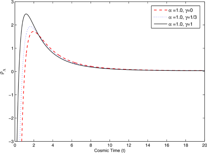

  

  Plot of DE density $\rho _{\Lambda }$ versus time $t$. For $\alpha =1.0$, $\gamma =0$, $\frac{1}{3}, 1, n=2$, $\phi _{0}=G_{0}= \omega =1$, $m_{1}=m_{2}=m_{3}=-1$

  In Fig. 6 to Fig. 8 we have plotted the density parameters $(\Omega _{m}, \Omega _{\Lambda },\Omega _{Total})$ with time for $\gamma =0$, $\gamma =\frac{1}{3}$ and $\gamma =1$. It is observed from figures that initially matter density parameter $\Omega _{m}$ and energy density parameter $\Omega _{\Lambda }$ have same values in all the three cases whereas the total energy density parameter $\Omega _{Total}$ increased from negative value to positive value and then remains constant for a period of time and then increasing sharply after that become negative.

  Fig. 6

  

  Plot of density parameters $(\Omega _{m}, \Omega _{\Lambda },\Omega )$ versus time $t$

  Fig. 7

  

  Plot of density parameters $(\Omega _{m}, \Omega _{\Lambda },\Omega )$ versus time $t$

  Fig. 8

  

  Plot of density parameters $(\Omega _{m}, \Omega _{\Lambda },\Omega )$ versus time $t$

• Table 1 describes the values of dynamics parameters that are directly related with the scale factor. It has been observed from table that the values of parameters are closed to standard $\Lambda$CDM model at present time i.e. $t_{0}=13.8$ Gyr.

  Table 1 Cosmological parameters in BVDP model (here $t_{0}=13.799$ Gyr)

6 Concluding remarks

Due to the present need of the problem we have constructed cosmological models in scalar-tensor theory of gravity proposed by Sáez and Ballester, here metric is coupled with a dimensionless scalar field. Such type of coupling provides a satisfied description of the weak field $(\phi )$. Under this motivation we had studied the Bianchi type-I cosmological models in Sáez-Ballester theory of gravity with BVDP. On the basis of the results obtained and discussed in Sect. 5 we may conclude that the behavior of DP indicated the transition phase of the universe. We may also infer that the universe which was decelerating in the past, accelerating at present time. It may also be seen that $\Lambda$ is decreasing function of time and converges to small positive value at late time, such nature of $\Lambda$ validate the results obtained through investigation by authors with recent observations. On the basis of above factual outcome we may say that our proposed universe model is decelerating for early time and indicate the transitional nature for late time. By choosing BVDP we found the generalize nature of research which has been already published by several authors with LVDP or constant DP in alternative theory of gravity.

References

Ade, P.A.R., et al.: Planck 2015 results: constraints on inflation. Astron. Astrophys. 594, A20 (2016)
Akarsu, Ȯ., Dereli, T.: Cosmological models with linearly varying deceleration parameter. Int. J. Theor. Phys. 51, 612 (2012)
Amendola, L.: Acceleration \(z > 1\)? Mon. Not. R. Astron. Soc. 342, 221–226 (2003)
Amirhashchi, H., Pradhan, A.: Accelerating dark energy models in bianchi Type-V space-time. Mod. Phys. Lett. A 26, 2266–2275 (2011)
Arbab, A.I.: Cosmological models with variable cosmological and gravitational ‘Constants’ and bulk viscous models. Gen. Relativ. Gravit. 29, 61 (1997)
Armendariz-Picon, C., et al.: A dynamical solution to the problem of a small cosmological constant and late time cosmic acceleration. Phys. Rev. Lett. 85, 4438–4441 (2000)
Berman, B.S.: Cosmological models with constant deceleration parameter. Gen. Relativ. Gravit. 20, 192 (1998)
Bolotin, Yu.L., et al.: Cosmology in terms of the deceleration parameter. Part I (2015). arXiv:1502.00811v1 [gr-qc]
Caldwell, R.R., Doran, M.: Cosmic microwave background and supernova constraints on quintessence: concordance regions and target models. Phys. Rev. D 69, 103517 (2004)
Canuto, V.M., Narlikar, J.V.: Cosmological tests of the Hoyle-Narlikar conformal gravity. Astrophys. J. 236, 6–23 (1980)
Chand, A., Mishra, R.K., Pradhan, A.: FRW cosmological models in Brans-Dicke theory of gravity with variable \(q\) and dynamical \(\Lambda \)- term. Astrophys. Space Sci. 361, 81 (2016)
Chawla, C., Mishra, R.K., Pradhan, A.: A new class of accelerating cosmological models with variable \(G\) and \(\Lambda \) in sáez and ballester theory of gravitation. Rom. J. Phys. 59, 12–25 (2014)
Dirac, P.A.M.: Cosmological models and the large numbers hypothesis. Proc. R. Soc. Lond. A 338, 439–446 (1974)
Dvali, G., et al.: 4D gravity on a brane in 5D Minkowski space. Phys. Lett. 485, 208–214 (2000)
Johri, V.B., Kalyani, D.: Cosmological models with constant deceleration parameter in Brans-Dicke theory. Gen. Relativ. Gravit. 26, 1217–1232 (1994)
Kamenshchik, A., et al.: An alternative to quintessence. Phys. Lett. B 511, 265–268 (2001)
Luis, O.P.: Exact cosmological solutions in the scalar-tensor theory with cosmological constant. Astrophys. Space Sci. 112, 175–183 (1985)
Mak, M.K., Harko, T.: Bianchi type-I universes with causal bulk viscous cosmological fluid. Int. J. Mod. Phys. D 11, 447–462 (2002)
Mishra, R.K., Chand, A.: Cosmological models in alternative theory of gravity with bilinear deceleration parameter. Astrophys. Space Sci. 361, 259 (2016)
Mishra, R.K., Chand, A.: A comparative study of cosmological models in alternative theory of gravity with LVDP & BVDP. Astrophys. Space Sci. 362, 140 (2017)
Mishra, R.K., Dua, H.: Bulk viscous string cosmological models in Sáez-Ballester theory of gravity. Astrophys. Space Sci. 364, 195 (2019)
Mishra, R.K., et al.: String cosmological models from early deceleration to current acceleration phase with varying G and \(\Lambda \). Eur. Phys. J. Plus 127, 137 (2012)
Padmanabhan, T.: Accelerated expansion of the universe driven by tachyonic matter. Phys. Rev. D 66, 021301 (2002)
Padmanabhan, T.: Cosmological constant–the weight of the vacuum. Phys. Rep. 380, 235–320 (2003)
Perlmutter, S., et al.: Discovery of a supernova explosion at half the age of the universe. Nature 391, 51–54 (1998)
Perlmutter, S., et al.: Measurements of \(\Omega \) and \(\Lambda \) from 42 high redshift supernovae. Astrophys. J. 517, 565 (1999)
Ramesh, G., Umadevi, S.: LRS bianchi type-II minimally interacting holographic dark energy model in Sáez-Ballester theory of gravitation. Astrophys. Space Sci. 361, 50 (2016)
Rao, V.U.M., Prasanthi, U.Y.D., Aditya, Y.: Plane symmetric modified holographic Ricci dark energy model in Sáez Ballester theory of gravitation. Results Phys. 10, 469–475 (2018)
Rasouli, S.M.M., Moniz, P.V.: Modified Sáez-Ballester scalar–tensor theory from 5D space–time. Class. Quantum Gravity 35, (1–23) (2018)
Rasouli, S.M.M., et al.: Late time cosmic acceleration in modified Sáez-Ballester theory. Phys. Dark Universe 27, 100446 (2020)
Ratra, B., Peebles, P.J.E.: Cosmological consequences of a rolling homogeneous scalar field. Phys. Rev. D 37, 3406 (1998)
Reddy, D.R.K., Naidu, R.L., Sobhan Babu, K., Naidu, K.D.: Bianchi type-V bulk viscous string cosmological model in Sáez-Ballester scalar tensor theory of gravitation. Astrophys. Space Sci. 349, 473–477 (2013)
Riess, A.G., et al.: Observational evidence from supernovae for an accelerating universe and a cosmological constant. Astron. J. 116, 1009 (1998)
Riess, A.G., et al.: The farthest known supernova: support for an accelerating universe and a glimpse of the epoch of deceleration. Astrophys. J. 560, 49–71 (2001)
Sáez, D., Ballester, V.J.: A simple coupling with cosmological implications. Phys. Lett. A 113, 467–470 (1986)
Sahni, V., et al.: Statefinder-a new geometrical diagnostic of dark energy. JETP Lett. 77, 201–206 (2003)
Schuecker, P., et al.: The Muenster Redshift Project. III. Observational constraints on the deceleration parameter. Astrophys. J. 496, 635 (1998)
Sharma, U.K., Zia, R., Pradhan, A.: Transit cosmological models with perfect fluid and heat flow in Sáez-Ballester theory of gravitation. J. Astrophys. Astron. 40, 2 (2019)
Spergel, D.N., et al.: First Year Wilkinson Microwave Anisotropy Probe (WMAP) observations: determination of cosmological parameters. Astrophys. J. Suppl. 148, 175–194 (2003)
Weinberg, S.: The cosmological constant problem. Rev. Mod. Phys. 61, 1 (1989)
Wesson, P.S.: In: Gravity, Particles and Astrophysics, Dordrecht, Holland (1980)
Acknowledgement
Author(s) are grateful to the editor and the anonymous referees for their constructive comments and suggestions to improve the research quality of this manuscript.
Author information
Authors and Affiliations
Corresponding author
Additional information
Publisher’s Note
Springer Nature remains neutral with regard to jurisdictional claims in published maps and institutional affiliations.
Rights and permissions
About this article
Cite this article
Mishra, R.K., Chand, A. Cosmological models in Sáez-Ballester theory with bilinear varying deceleration parameter. Astrophys Space Sci 365, 76 (2020). https://doi.org/10.1007/s10509-020-03790-w
Received:
Accepted:
Published:
DOI: https://doi.org/10.1007/s10509-020-03790-w