
Abstract
The paper is concerned with a predator-prey diffusive system subject to homogeneous Neumann boundary conditions, where the growth rate \((\frac{\alpha}{1+\beta v})\) of the predator population is nonlinear. We study the existence of equilibrium solutions and the long-term behavior of the solutions. The main tools used here include the super-sub solution method, the bifurcation theory and linearization method.
1 Introduction
We consider existence, nonexistence and stability of steady-state solutions of the following reaction-diffusion system,
where \(\varOmega\) is a bounded domain in \(R^{N}\) with a smooth boundary \(\partial\varOmega\), \(\Delta\) is the Laplacian operator in \(R^{N}\) and \(a, d\) denote the intrinsic growth rate of prey population and the constant predator population mortality, respectively. \(a,b,m,\alpha,d,c\) and \(d_{1}, d_{2}\) are positive constants. One can refer to [14] and the references therein for the corresponding biological meaning about the model. In addition, \(n\) is the outward unit normal vector of the boundary \(\partial\varOmega\), the homogeneous Neumann boundary conditions mean that (1.1) is self-contained and has no population flux across the boundary \(\partial \varOmega\), which implies that the system is an insular system.
The corresponding steady-state system to (1.1) is
Equation (1.2) with homogeneous Dirichlet boundary conditions was studied by Yang et al. [14], where the existence, stability and exact number of positive solution were given when \(m\) is large. In particular, we note that \(a, \alpha/(1 + \beta v)\) are the growth rate of the prey and predator population respectively, where \(\beta\) can be understood as the strength of intraspecific interference. Reference [14] also charactered the effect of the parameter \(\beta\) on the population density, which presents that the population density of \(u\) is decreasing as \(\beta\) decreases, but the population density of \(v\) is in the opposite direction. It is worth stressing that, \(\alpha/(1+\beta v)\) is a Beverton-Holt-like function and can be founded in [1, 3, 4, 13], however, the growth rate function only appeared in discrete models up to now, such as \(X_{n+1}=\frac{AX_{n}}{1+BX_{n}}, \ n=0,1,2,\ldots\) . (See [13]), where \(X\) is population size at time \(n\) and \(A,B\) are constants. The previous considered growth function is linear, such as the well-known Logistic model. However, the growth rate is related to the density of the population in numerous biological phenomena, i.e., the nonlinear growth rate is of great ecological significance.
This paper is organized as follows. Section 2 is devoted to studying the existence and nonexistence of positive steady states. In Sect. 3, we investigate local and global stability of various steady states. We illustrate some results with numerical simulations in Sect. 4.
2 Existence and Nonexistence of Positive Steady States
In this section, we mainly consider the existence and nonexistence of positive steady states of (1.1), i.e., the positive solution of (1.2).
Lemma 2.1
(See [8, Proposition 2.2])
Assume that \(g\in C(\overline {\varOmega}\times R^{1})\).
-
(1)
Assume that \(w\in C^{2}(\varOmega)\cap C^{1}(\overline{\varOmega})\) and satisfies: \(\Delta w(x)+g(x,w(x))\geq0\) in \(\varOmega\), \(\frac{\partial w}{\partial n}\leq0\) on \(\partial\varOmega\). If \(w(x_{0})=\max_{\overline{\varOmega}} w\), then \(g(x_{0},w(x_{0}))\geq 0\).
-
(2)
Assume that \(w\in C^{2}(\varOmega)\cap C^{1}(\overline{\varOmega})\) and satisfies: \(\Delta w(x)+g(x,w(x))\leq0\) in \(\varOmega\), \(\frac{\partial w}{\partial n}\geq0\) on \(\partial\varOmega\). If \(w(x_{0})=\min_{\overline{\varOmega}} w\), then \(g(x_{0},w(x_{0}))\leq0\).
Lemma 2.2
Assume that \(0< d-\frac{ac}{1+ma}<\alpha\). If \((u,v)\) is a nonnegative solution of (1.2), then
In addition, if \(\alpha>d\), then \(v\geq\frac{\alpha-d}{\beta d}\).
Proof
Let \((u,v)\) be the a nonnegative solution of (1.2). We denote \(u(x_{0})=\max_{\overline{\varOmega}} u\) and \(v(y_{0})=\max_{\overline{\varOmega}} v\) for some \(x_{0}, y_{0}\in\overline{\varOmega}\). By virtue of Lemma 2.1, we have
It follows from inequality (2.1) that \(u(x)\leq a, x\in\overline {\varOmega}\). Since \(0< d-\frac{ac}{1+ma}<\alpha\) and \(u\leq a\), it follows form inequality (2.2) that \(v(y_{0})\leq\frac{\alpha-d+\frac {ac}{1+ma}}{\beta(d-\frac{ac}{1+ma})}\equiv M_{0}\). Therefore, \(v(x)\leq M_{0}, x\in\overline{\varOmega}\).
Similarly, if \(\alpha>d\) and set \(v(y_{1})=\min_{\overline{\varOmega}} v\) for some \(y_{1}\in\overline{\varOmega}\), then by virtue of Lemma 2.1 again, we have \(\frac{\alpha}{1+\beta v(y_{1})}-d+\frac {cu(y_{1})}{1+mu(y_{1})}\leq0\). One can see that \(v\geq\frac{\alpha -d}{\beta d}\). This completes the proof. □
Remark 1
In fact, if \(d>\frac{ac}{1+ma}\) and \((u,v)\) is a positive solution of (1.2), then
Let \(\lambda_{1}(\mu,q)\), where \(\mu>0\) and \(q\in C(\overline{\varOmega })\), be the principal eigenvalue of the operator \(-\mu\Delta+q(x)\) in \(\varOmega\) subject to the homogeneous Neumann boundary condition. Denote \(\lambda_{1}(\mu,0)\) by \(\lambda_{1}(\mu)\) and note that \(\lambda _{1}(\mu)=0\). Consider the eigenvalue problem
whose eigenvalues can be listed as \(0=\lambda_{1}<\lambda_{2}<\lambda _{3}\cdots\) with the associated eigenfunction \(\psi_{i}, i=1,2,3\cdots\).
Theorem 2.1
Assume that \(d-\frac{ac}{1+ma}>0\). If \(\alpha\leq d-\frac{ac}{1+ma}\) and \((u,v)\) is a nonnegative solution of (1.2), then \(v(x)\equiv0\), i.e., \((a,0)\) is the unique nontrivial solution of (1.2).
Proof
Let \((u,v)\) be a nonnegative solution of (1.2). If \(v(x)\not\equiv0\), then \(v(x)>0\) by the maximum principle. Define \(q(x)=d-\frac{\alpha}{1+\beta v}-\frac{cu}{1+mu}\). It follows from (1.2) that \(\lambda_{1}(d_{2},q)=0\). If \(\alpha \leq d-\frac{ac}{1+ma}\), then
By a comparison, \(\lambda_{1}(d_{2},q)>\lambda_{1}(d_{2})=0\), which is a contradiction with the fact that \(\lambda_{1}(d_{2},q)=0\). We have thus proved the theorem. □
Theorem 2.2
Assume that \(d>\frac{ac}{1+ma}\), then (1.2) has no non-constant positive solution if \(d_{1}>(a+\frac{cM_{0}}{2})/\lambda_{2}\) and \(d_{2}>(\frac{cM_{0}}{2}+\alpha-d+\frac{ac}{1+ma})/\lambda_{2}\), where \(M_{0}\) is defined in Lemma 2.2 and \(\lambda_{2}\) is the first positive eigenvalue of problem (2.3).
Proof
Assume \((u,v)\) is a positive solution of (1.2) and let \(\overline {\phi}=\frac{1}{|\varOmega|}\int_{\varOmega}\phi dx\), it is necessary that \(\alpha>d-\frac{ac}{1+ma}\). Multiplying the first equation of (1.2) by \((u-\overline{u})\) and the second by \((v-\overline{v})\) and evaluating integrals on \(\varOmega\), we have
By Lemma 2.2, the mean inequality and Poincaré inequality,
Obviously, if \(d_{1}>(a+\frac{cM_{0}}{2})/\lambda_{2}\) and \(d_{2}>(\frac {cM_{0}}{2}+\alpha-d+\frac{ac}{1+ma})/\lambda_{2}\), then \((u,v)=(\overline{u},\overline{v})\). □
In order to analyze the existence of positive constant solutions to (1.2), i.e., the positive solution of the following algebraic equation (2.4),
we assume that the following condition holds:
- (H):
-
\(ma=1\) and \(d(b+\beta a)=\alpha b\).
Under the condition (H), the equation in terms of \(u\) can be obtained by eliminating \(v\):
where \(v=(a-u)(1+mu)/b\), \(\overline{a}=\beta m(dm+c), \overline {b}=\beta dm\) and \(\overline{c}=-(b+\beta a)c\). Let \(A=\overline {b}^{2}-\overline{a}\overline{c}\), \(B=\overline{b}\overline{c}\), \(C=\overline{c}^{2}\) and \(\varLambda=B^{2}-4AC\). It is easy to check that \(A=\beta^{2}d^{2}m^{2}+3\beta cm(dm+c)(b+\beta a)>0\), \(B=-\beta cdm(b+\beta a)<0\), \(C=(b+\beta a)^{2}c^{2}\) and
- Observation 1:
-
If \(\varLambda>0\), i.e., \(\beta d^{2}m[(b+\beta a)c-4]>12(dm+c)(b+\beta a)c\), then (2.5) has no positive real solutions, i.e., (1.2) has no positive constant solution.
- Observation 2:
-
If \(\varLambda=0\), i.e., \(\beta d^{2}m[(b+\beta a)c-4]=12(dm+c)(b+\beta a)c\), then (2.5) has two same positive real solutions \(u_{1,2}=u^{*}=-\frac{B}{2A}=\frac{(b+\beta a)cd}{2[\beta d^{2}m+3c(dm+c)(b+\beta a)]}\). One see that (1.2) has a unique positive constant solution \((u^{*},v^{*})\), where \(v^{*}=(a-u^{*})(1+mu^{*})/b>0\) by the condition (H).
Theorem 2.3
Assume that \(\alpha>d-\frac{ac}{1+ma}>0\) and \(M_{1}=\frac{\alpha -d+ac/(1+ma)}{\beta(d-ac/(1+ma))}\). If \(a>bM_{1}\) and \(\alpha>d-\frac{c(a-bM_{1})}{1+m(a-bM_{1})}\), then (1.2) has at least one positive solution.
Proof
First, we rewrite (1.2) in the form as follows:
where \(f(u,v)=u(a-u)-\frac{buv}{1+mu}\) and \(g(u,v)=v(\frac{\alpha }{1+\beta v}-d)+\frac{cuv}{1+mu}\). For all \(u\geq0\) and \(v\geq0\), we have \(\frac{\partial f}{\partial v}=-\frac{bu}{1+mu}\leq0\) and \(\frac{\partial g}{\partial u}=-\frac{cv}{(1+mu)^{2}}\geq0\), that is to say, (2.6) is a so-called mixed quasi-monotonic system (See [9]). Now we want to construct a pair of upper and lower solutions \(\overline {U}=(\overline{u}(x),\overline{v}(x))\) and \(\underline{U}=(\underline {u}(x),\underline{v}(x))\). By the definitions of upper and lower solutions (See [9]), it suffices to find \(\overline{U}=(\overline{u}(x),\overline{v}(x))\) and \(\underline{U}=(\underline{u}(x),\underline{v}(x))\) satisfying \(\underline{U}\leq\overline{U}\) and
Let \(\overline{u}(x)=a\). Then the left side of (2.7b) holds for any \(\underline{v}(x)\geq0\). By the hypotheses, we can take \(\overline{v}(x)=M_{1}=\frac{\alpha -d+ac/(1+ma)}{\beta(d-ac/(1+ma))}(>0)\), then the left side of (2.7c) holds.
Now, the right side of (2.7b) becomes \(-d_{1}\Delta\underline {u}-\underline{u}(a-\underline{u}-\frac{bM_{1}}{1+m\underline{u}})\leq0\). We claim that the boundary value problem
has a positive solution. In fact, since \(a>bM_{1}\), it is easy to verify that \(a\) and \(a-bM_{1}\) are a pair of upper and lower solutions of (2.8) and thus (2.8) has a positive solution \(w(x)\) satisfying \(a-bM_{1}\leq w(x)\leq a\). Take \(\underline{u}=w(x)(\leq a)\). Since \(\underline{u}(x)\) has a lower bound \(a-bM_{1}\), the right side of (2.7c) is satisfied if we take \(\underline{v}(x)\) to be a small positive constant. So we have constructed a pair of upper and lower solutions \(\overline {U}=(\overline{u}(x),\overline{v}(x))\) and \(\underline{U}=(\underline {u}(x),\underline{v}(x))\) satisfying \(\overline{U}(x)\geq\underline{U}(x)\), which yields the existence of positive solution \((u(x),v(x))\) to (1.2) and
The theorem is proved. □
Assume that \(d-\frac{ac}{1+ma}>0\) and we consider the bifurcation at \((\widetilde{\alpha};a,0)\), where \(\widetilde{\alpha}=d-\frac{ac}{1+ma}\).
Theorem 2.4
Assume that \(d-\frac{ac}{1+ma}>0\). Then for \(a>0\) fixed and \(\delta>0\) small, there exists a continuum \(\varGamma_{1}\) of solution of (1.2), where \(\varGamma_{1}=\{(\alpha(s);a-w(s),v(s)): s\in[0,\delta)\}\) with \(\alpha(0)=d-\frac{ac}{1+ma}, w(s)=\frac{b}{1+ma}s+o(|s|)\) and \(v(s)=s+o(|s|)\). Moreover, the bifurcation \(\varGamma_{1}\) is supercritical.
Proof
For \(p>1\), let \(X=\{u\in W^{2,p}(\varOmega): \frac{\partial u}{\partial n}=0, x\in\partial\varOmega\}^{2}\), \(Y=L^{p}(\varOmega)^{2}\). We take the variables \(w=a-u\) and define \(G(\alpha;w,v): \mathbb{R}\times X\rightarrow Y\) by
where \(h(u,v)=\frac{uv}{1+mu}\). By using a simple calculation,
where \(h_{u}(u,v)=\frac{v}{(1+mu)^{2}}\), \(h_{v}(u,v)=\frac{u}{1+mu}\), \(h_{uu}(u,v)=-\frac{2mv}{(1+mu)^{3}}\) and \(h_{uv}(u,v)=\frac{1}{(1+mu)^{2}}\).
At \((\alpha;w,v)=(\widetilde{\alpha};0,0)\), it is easy to check that the kernel \(\mathcal{N}(G_{(w,v)}(\widetilde{\alpha};0,0))=\mathrm {span}\{(\frac{b}{1+ma},1)\}\), the range \(\mathcal {R}(G_{(w,v)}(\widetilde{\alpha};0,0))=\{(f,g)^{T}\in Y: \int_{\varOmega }g(x)dx=0\}\), and \(G_{\alpha(w,v)}(\widetilde{\alpha};0,0)[\frac {b}{1+ma},1]=(0,1)^{T}\notin\mathcal{R}(G_{(w,v)}(\widetilde{\alpha };0,0))\) since \(\int_{\varOmega}1dx=|\varOmega|>0\). By applying the results of [2] or [12, Theorem 13.4], the set of solutions to (1.2) near \((\widetilde{\alpha};0,0)\) is a smooth carve
with \(\delta>0\) small, \(\alpha(0)=d-\frac{ac}{1+ma}, w(s)=\frac {b}{1+ma}s+o(|s|), v(s)=s+o(|s|)\). By [7, Corollary 2.3],
where \(l\) is a linear functional on \(Y^{2}\) defined as \(\langle l,[f,g]\rangle=\int_{\varOmega}g(x)dx\). This yields that the bifurcation \(\varGamma_{1}\) at \((\widetilde{\alpha};0,0)\) is supercritical. □
By the unilateral global bifurcation theorem developed by López-Gómez, one can see [5, Theorem 6.4.3] or [6, Theorem 2.2] for the details, we study the global bifurcation at \((\widetilde{\alpha};0,0)\). Let \(P=\{u\in W^{2,p}(\varOmega): u>0, x\in\overline{\varOmega}\}\), which is the nature positive cone in \(X\), and then \(P^{2}\) is the nature positive cone in \(X^{2}\).
Theorem 2.5
Suppose that \(d-\frac{ac}{1+ma}>0\) and \(\widetilde{\alpha}=d-\frac{ac}{1+ma}\).
-
(1)
For \(a>0\) fixed and \(\alpha\in(0,d]\), there exists a component \(\mathcal{C}^{+} (\supset\varGamma_{1})\) of solution to (1.2) bifurcating from \((\alpha;u,v)\) at \((\widetilde{\alpha};a,0)\), and the curve \(\mathcal{C}^{+}\) joints from \((\widetilde{\alpha};a,0)\) to \((\overline{\alpha};0,0)\), where \(\overline{\alpha}=d\).
-
(2)
For \(a\in[0,\infty)\) and \(\alpha\in[d,\infty)\), there exists a component \(\varGamma_{2} (\cap\,\mathcal{C}^{+}=\emptyset)\) of positive solution to (1.2) bifurcating from \((a,d;u,v)\) at \((0,\overline {\alpha};0,0)\).
Proof
From the proof of Theorem 2.4, it follows that all the conditions in [5, Theorem 6.4.3] hold. This yields that there exists a component \(\mathcal{C}^{+}\supset\varGamma_{1}\) of solution to (1.2) bifurcating at \((\widetilde{\alpha};a,0)\) and \(\mathcal {C}^{+}\) satisfies one of the following alternatives:
-
(i)
\(\mathcal{C}^{+}\) is unbounded in \(\mathbb{R}\times X\).
-
(ii)
There exists \(\widehat{\alpha}\) such that \((\widehat{\alpha };a,0)\in\mathcal{C}^{+}\), where \(\widetilde{\alpha}\neq\widehat{\alpha }\in\{\alpha: \mathrm{dim}\mathcal{N}(G_{(w,v)}(\alpha;0,0))\geq1\}\).
-
(iii)
\(\mathcal{C}^{+}\) contains a point \((\alpha;u,v)\in(0,d]\times (Z\setminus\{(a,0)\})\), where \(Z\) is the complement of \(\mathcal {N}(G_{(w,v)}(\widetilde{\alpha};0,0))\) in \(X^{2}\) and can be taken as \(\mathcal{R}(G_{(w,v)}(\widetilde{\alpha};0,0))\) in the proof of Theorem 2.4.
(1) Case \(a>0\) fixed and \(\alpha\in(0,d]\). Assume that \(\mathcal {C}^{+}\setminus(\widetilde{\alpha};a,0)\subset P^{2}\). By Lemma 2.2, (i) is impossible. Recall that \(\mathcal {R}(G_{(w,v)}(\widetilde{\alpha};0,0))=\{(f,g)\in Y: \int_{\varOmega }g(x)dx=0\}\), so (iii) is also impossible. It is easy to verity that positive solutions of (1.2) bifurcate from the semi-trivial solution curve \(\{(\alpha;a,0)\}\) if and only if \(\alpha=\widetilde {\alpha}\), i.e., (ii) is impossible. Therefore, \(\mathcal {C}^{+}\setminus(\widetilde{\alpha};a,0)\not\subset P^{2}\) and there exists \((\overline{\alpha};\overline{u},\overline{v})\in\{\mathcal {C}^{+}-(\widetilde{\alpha};a,0)\}\cap\partial P^{2}\) with \(0\leq \overline{\alpha}\leq d\), which is the limit of a sequence \(\{(\alpha _{i};u_{i},v_{i})\}\subset\mathcal{C}^{+}\cap P^{2}\) with \(u_{i}>0, v_{i}>0\) on \(\overline{\varOmega}\). From the maximum principle, it follows that \((\overline{\alpha};\overline{u},\overline{v})\) must be one of the three cases: \(\overline{u}\equiv0,\overline{v}\equiv0\) or \(\overline {u}>0,\overline{v}\equiv0\) or \(\overline{u}\equiv0,\overline{v}>0\).
Suppose that \(\overline{u}\equiv0,\overline{v}>0\). It is easy to check that \(\overline{v}=\frac{\overline{\alpha}-d}{\beta d}>0\), i.e., \(\overline{\alpha}>d\), which is a contradiction with \(\overline{\alpha }\leq d\).
Suppose that \(\overline{u}>0,\overline{v}\equiv0\). It is easy to check that \(\overline{u}\equiv a\). Let \(\widetilde {v}_{i}=v_{i}/\|v_{i}\|_{\infty}\) and assume \(\widetilde {v}_{i}\rightarrow\widetilde{v}>0\). Then \(\widetilde{v}\) satisfies
From the above equation, we have \(\widetilde{v}=1\) and \(\overline{\alpha }=d-\frac{ac}{1+ma}=\widehat{\alpha}\), which is a contradiction with (ii).
Therefore, we must have \(\overline{u}\equiv0,\overline{v}\equiv0\). Similarly, let \(\widetilde{v}_{i}=v_{i}/\|v_{i}\|_{\infty}\) and assume \(\widetilde{v}_{i}\rightarrow\widetilde{v}>0\). Then \(\widetilde{v}\) satisfies
then \(\widetilde{v}=1\) and \(\overline{\alpha}=d\), i.e., the component \(\mathcal{C}^{+}\) joints from \((\widetilde{\alpha};a,0)\) to \((\overline {\alpha};0,0)\), where \(\widetilde{\alpha}=d-\frac{ac}{1+ma}\) and \(\overline{\alpha}=d\).
(2) Case \(a\in[0,\infty)\) and \(\alpha\in[d,\infty)\). Recall the proof of Theorem 2.4 and define \(H(a,\alpha;u,v): \mathbb{R}^{2}\times X\rightarrow Y\) by
By using a simple calculation, \(\mathcal{N}(H_{(u,v)}(0,d;0,0))=\mathrm {span}\{(1,0)^{T},(0,1)^{T}\}\) and
Decompose \(X\) as \(X=X_{1}+X_{2}\) and \(Y=Y_{1}+Y_{2}\), where \(X_{1}=Y_{1}=\mathcal{N}(H_{(u,v)}(0,d;0,0))\), \(Y_{2}=\mathcal {R}(H_{(u,v)}(0,d;0,0))\) and \(X_{2}=\mathcal {R}(H_{(u,v)}(0,d;0,0))\cap Y\). Assume that \((u,v)^{T}=s\bigl( {\scriptsize\begin{matrix}{}\cos\omega+w_{1} \cr \sin\omega+w_{2}\end{matrix}} \bigr)\) with \((w_{1},w_{2})\in X_{2}\), \(\omega\in(0,\pi/2)\) fixed. Let \(a=\gamma, \alpha=d+\tau\), and define \(K(w_{1},w_{2},\gamma,\tau;s): X_{2}\times\mathbb{R}^{3}\rightarrow Y\) by
where \(u=s(\cos\omega+w_{1}),v=s(\sin\omega+w_{2})\). By a simple calculation, \(K(0,0,0,0;0)=0\) and
which is an isomorphism from \(X_{2}\times\mathbb{R}^{2}\) to \(Y\). By the implicit function theorem, there exists a continuous curve \((w_{1}(s),w_{2}(s),\gamma(s),\tau(s))\) defined in a neighborhood of 0, such that
Now, set \(u(s)=s(\cos\omega+w_{1}), v(s)=s(\sin\omega+w_{2}), a(s)=\gamma(s)\) and \(\alpha(s)=d+\tau(s)\). Substituting \(u(s),v(s), a(s)\) and \(\alpha(s)\) in \(H(a,\alpha;u,v)=0\), dividing \(H\) by \(s\) and then taking derivative at \(s=0\), we have
In fact, if we chose \(\omega\in(0,\pi/2)\) such that \(\tan\omega>\frac {c}{\beta d}\), then \(\tau'(0)>0\). Therefore, for \(s>0\) small and \(\omega \in(0,\pi/2)\) satisfying \(\tan\omega>\frac{c}{\beta d}\), \(\varGamma_{2}=\{ (a(s),\alpha(s);u(s),v(s)): s>0 \ \text{small}\}\) is a curve of positive solution to \(H(a,\alpha;u,v)=0\). □
Remark 2
The results in Theorem 2.5 can be shown by Fig. 1. In other words, we construct a component from \((\widetilde{\alpha };a,0)\) to \((\overline{\alpha};0,0)\) (taking \(\alpha\) as bifurcation parameter), and there occurs a new bifurcation \(\varGamma_{2}\) bifurcating from \((a,d;u,v)\) at \((0,\overline{\alpha};0,0)\) (taking \(a\) and \(\alpha \) as bifurcation parameters simultaneously). See the right sub-figure, the whole curve, for details.

The possible bifurcation diagram for Theorem 2.5. Left: \(\mathcal{C}^{+} (\supset\varGamma_{1})\) jointing from \((\widetilde {\alpha};a,0)\) to \((\overline{\alpha};0,0)\), Right (green part): \(\varGamma _{2}\) bifurcating from \((a,d;u,v)\) at \((0,\overline{\alpha};0,0)\) (Color figure online)
Remark 3
-
(1)
Theorems 2.3–2.5 all show the existence of positive solution to (1.2), however, we do not know the existed positive solutions are constant or functions of \(x\).
-
(2)
Under the condition (H), assume that \(a>0, \alpha>d\) and \(|a|,|\alpha -d|\ll1\). It follows from Observation 1 and Theorem 2.5 that \(\varGamma_{2}\setminus\{(0,\overline{\alpha};0,0)\}\) consists of non-constant positive solutions to (1.2), if \(\beta d^{2}m[(b+\beta a)c-4]>12(dm+c)(b+\beta a)c\). According to the condition (H) and the conditions “\(a>0, \alpha>d\) and \(|a|,|\alpha -d|\ll1\)”, we need to guarantee the inequation \(\beta d^{2}m[(b+\beta a)c-4]>12(dm+c)(b+\beta a)c\) holds if \(m\rightarrow\infty\) and \(\beta\) is bounded. In fact, we only need to guarantee the inequation \(\beta d(bc-4)>12bc\) holds if \(\beta\) is bounded. Hence, if we chose “\(d\) and \(b\)” (or “\(d\) and \(c\)”) sufficiently large, there exists non-constant positive solution to (1.2). The analysis procedure is as follows:
-
1.
(H) \(ma=1\) and \(d(b+\beta a)=\alpha b\).
-
2.
\(a>0, \alpha>d\) and \(|a|,|\alpha-d|\ll1\).
-
3.
\(\beta d^{2}m[(b+\beta a)c-4]>12(dm+c)(b+\beta a)c\).
-
1.
Comparing conditions 1 and 2, we need to guarantee condition 3 holds if \(m\rightarrow\infty\) and \(\beta\) is bounded. Note that
- A::
-
\(\beta d^{2}m[(b+\beta a)c-4]>12(dm+c)(b+\beta a)c, \text{ if $m\rightarrow\infty$ and $\beta$ is bounded}\);
- B::
-
\(\beta d^{2}(bc-4)+\frac{\beta^{2}d^{2}c}{m}>12dbc+\frac {12c(db+d\beta+c\beta a)}{m}, \text{ if $m\rightarrow\infty$ and $\beta $ is bounded}\);
- C::
-
\(\beta d(bc-4)>12bc, \text{ if $\beta$ is bounded}\);
- D::
-
\(d, b\) sufficiently large or \(d, c\) sufficiently large.
One can see that if \(ma=1\), then \(A\Leftrightarrow B\). In fact, if \(m\rightarrow\infty\), then \(B\Leftarrow C\), and \(C\Leftarrow D\) is obvious.
3 Stability of the Steady State Solutions
In this section, we talk about the stability of the nonnegative solution of (1.2).
Now, we consider the steady state solution of (1.1), i.e., the constant solution of (1.2). It is easy to see that (1.2) may have the following nonnegative solutions: \(S_{1}=(u,v)=(0,0)\), \(S_{2}=(u,v)=(a,0)\), \(S_{3}=(u,v)=(0,\frac{\alpha -d}{\beta d})\) if \(\alpha>d\), \(S_{4}=(u,v)=(\rho,\sigma)\), where \((\rho,\sigma)\) is the positive algebraic solution to (2.4) and \(S_{5}=(u,v)=(u(x),v(x))\), where \(u(x),v(x)\) are two positive functions.
Remark 4
It is possible for the existence of positive constant solution to (1.2) in the form of \(S_{4}\) and \(S_{5}\). One can see Observation 2 for the former and see Remark 3 2) for the latter.
It is well-known (see [11]) that the stability question for \(S_{i}=(u_{i},v_{i})\) is answered by considering the spectrum of the linearized operator around each \(S_{i}\).
Theorem 3.1
-
(1)
\(S_{1}=(0,0)\) is unstable;
-
(2)
\(S_{2}=(a,0)\) is unstable if \(\alpha-d+\frac{ac}{1+ma}>0\) and stable if \(\alpha-d+\frac{ac}{1+ma}<0\);
-
(3)
Assume that \(\alpha>d\). If \(a<\frac{b(\alpha-d)}{\beta d}\), then \(S_{3}=(0,\frac{\alpha-d}{\beta d})\) is stable.
Proof
Here, we will prove only 2), the other cases can be studied in a similar manner. From the linearization principle, the stability of \(S_{2}=(a,0)\) is determined by studying the following spectral problem
Since (3.1) is not completely coupled, we only need to consider the following two eigenvalue problems (the eigenvalue of (3.1) is real)
and
Assume that \(\alpha-d+\frac{ac}{1+ma}>0\). The principal eigenvalue \(\widetilde{\lambda}_{1}\) of (3.2) is positive (\(\widetilde {\lambda}_{1}=\alpha-d+\frac{ac}{1+ma}>0\)) and the associated eigenfunction \(\widetilde{w}_{2}>0\). Let \(\widetilde{w}_{1}\) be the unique solution of
Then \(\widetilde{\lambda}_{1}=\alpha-d+\frac{ac}{1+ma}>0\) is a eigenvalue of (3.1) with the associated eigenfunction \((\widetilde {w}_{1},\widetilde{w}_{2})\), i.e., (3.1) has a eigenvalue whose real part is greater than 0. Therefore, \(S_{2}=(a,0)\) is unstable.
Assume that \(\alpha-d+\frac{ac}{1+ma}<0\). Let \(\overline{\lambda}_{1}\) be the largest eigenvalue of (3.1) and the associated eigenfunction \((\overline{w}_{1},\overline{w}_{2})\). If \(\overline {w}_{2}\not\equiv0\), then \(\overline{\lambda}_{1}\) is also the eigenvalue of (3.2). One see that the largest eigenvalue of (3.2) is \(\alpha-d+\frac{ac}{1+ma}\ (<0)\), hence, \(\overline{\lambda }_{1}<0\). If \(\overline{w}_{2}\equiv0\), then \(\overline{w}_{1}\not \equiv0\) and \((\overline{\lambda}_{1},\overline{w}_{1})\) are the eigenvalue and the associated eigenfunction of
Similarly as above, we also have \(\overline{\lambda}_{1}<0\). Therefore, \(S_{2}=(a,0)\) is stable. □
Theorem 3.2
Assume that \(0< d-\frac{ac}{1+ma}<\alpha\) and \(S_{4}=(\rho,\sigma)>0\) exists (see Observation 2). If \(a>bM_{0}\) and \(1+m(a-2bM_{0})\geq0\), then \(S_{4}\) is stable. Here, \(M_{0}\) is defined in Lemma 2.2.
Proof
The linearized operator of (1.1) at \(S_{4}=(\rho,\sigma)\) can be expressed by \(D\Delta W+\mathcal{L}W\) with the domain \(\{(\phi,\psi)\in H^{2}(\varOmega)\times H^{2}(\varOmega): \frac{\partial\phi}{\partial n}=\frac{\partial\psi}{\partial n}=0\}\), where
Let \(C_{i}=\mathcal{L}-\lambda_{i}D\). Note that \(S_{4}\) is stable if and only if each \(C_{i}\) has two eigenvalues with negative real parts. The eigenvalues \(\mu_{1,2}\) of \(C_{i}\) are determined by
It suffices to prove that
One see that
Recall that \(B<0, E>0\). Now, we claim that \(A\leq0\), i.e., \(a-2\rho -\frac{b\sigma}{(1+m\rho)^{2}}\leq0\). By the definition of \((\rho,\sigma)\), we have \((a-\rho)(1+m\rho)=b\sigma \). Equation (1.2) has a positive solution \((\rho,\sigma)\), it is necessary that \(a-bM_{0}<\rho<a\), where \(M_{0}\) is defined in Lemma 2.2. We obtain that
We need only to prove that \(\frac{\rho+a+2m\rho^{2}}{1+m\rho}\geq a\), i.e., \(1+2m\rho\geq ma\), which is satisfied since \(\rho>a-bM_{0}\) and \(1+m(a-2bM_{0})\geq0\). This proves the theorem. □
Theorem 3.3
Assume that \(c/m< d<\alpha\) and \(a<\frac{b(\alpha-d)}{\beta d}<\frac {1}{m}\). Then for any nonnegative initial functions \(u_{0}(x)\) and \(v_{0}(x)\) such that for some \(\sigma\geq0, v(x,\sigma)\geq\frac{\alpha -d}{\beta d}\), the corresponding solution \((u(x,t),v(x,t))\) of (1.2) satisfies \((u(x,t),v(x,t))\rightarrow(0,\frac{\alpha-d}{\beta d})\) as \(t\rightarrow\infty\).
Proof
We construct a pair of upper and lower solutions of (1.2) in the form of \((\overline{u},\overline{v}), (\underline{u},\underline{v})\), where \(\overline{u}>0, \overline{v}>\underline{v}\) are positive constants to be determined and \(\underline{u}=0\). So, we should have
Since \(c/m< d<\alpha\), these inequalities are satisfied if \(\underline {v}=\frac{\alpha-d}{\beta d}, \overline{u}\geq a, \overline{v}\geq \frac{\alpha-d+\frac{c\overline{u}}{1+m\overline{u}}}{\beta(d-\frac {c\overline{u}}{1+m\overline{u}})}\). Now we take \(\overline{U}^{(0)}=(\overline{u},\overline{v})\) and \(\underline{U}^{(0)}=(\underline{u},\underline{v})\) as the initial iterations and construct two sequences \(\{\overline{U}^{(k)}\}\equiv\{ (\overline{u}^{(k)},\overline{v}^{(k)})\}\) and \(\{\underline{U}^{(k)}\} \equiv\{(\underline{u}^{(k)},\underline{v}^{(k)})\}\). Then these sequences possess the monotone property \((\underline{u},\underline {v})\leq\underline{U}^{(k)}\leq\underline{U}^{(k+1)}\leq\overline {U}^{(k+1)}\leq\overline{U}^{(k)}\leq(\overline{u},\overline{v})\), and converge to their respective limits \(\lim_{k\rightarrow\infty }\overline{U}^{(k)}=(\widetilde{u},\widetilde{v})\) and \(\lim_{k\rightarrow\infty}\underline{U}^{(k)}=(0,\widehat{v})\), which satisfy the relations
Now we show that \(\widetilde{u}\equiv0\). If not, by the maximum principle, we have \(\widetilde{u}(x)>0\). Then \(\widetilde{\lambda }_{1}=0\) is the principal eigenvalue of the problem
Since \(\widehat{v}\geq\underline{v}=\frac{\alpha-d}{\beta d}\), we have \(q(x)\geq\frac{b(\alpha-d)}{\beta d}-a>0\) from the assumption. Therefore, a comparison with problem (3.9), we know that the following eigenvalue problem
has the principal eigenvalue \(\widehat{\lambda}_{1}\), which is non-positive. In fact, \(\widehat{\lambda}_{1}=\frac{b(\alpha-d)}{\beta d}-a>0\). This is a contradiction. Therefore, we have \(\widetilde{u}\equiv0\). From (3.7) and (3.8), one see that \(\widetilde{v}=\widehat {v}=\frac{\alpha-d}{\beta d}\). Therefore from [15, Corollary 3.1] or [10, Corollary 2.2], we know that if for some \(\sigma\geq0, v(x,\sigma)\geq\frac{\alpha-d}{\beta d}\), then the corresponding solution \((u(x,t),v(x,t))\) of (1.2) satisfies \((u(x,t),v(x,t))\rightarrow(0,\frac{\alpha-d}{\beta d})\) as \(t\rightarrow\infty\). □
Remark 5
From Theorem 3.3, one see that if the population of the native predators attains certain level at some time, then the native preys will be extinct after a long time.
4 Numerical Simulation
The goal of this section is to present the results of numerical simulations which complement the analytic results in Sect. 3. We simulate the corresponding system (1.1) in the one-dimensional space domain. Without loss of generality, we take \(\varOmega=(0,2\pi)\). We perform the initial-boundary-value problem numerically based on the Crank-Nicholson scheme. In each simulation, the figures are plotted at sufficiently final time (here, we take \(T=50\)), which allow us to regard the solutions as steady states. In the finite difference scheme, we take the temporal axis with grid spacing \(\Delta t=50/99\) and the spatial axis with grid spacing \(\Delta x=2\pi/49\).
Several parameters are common for all simulations: \(b=0.05, c=0.03, d=0.5, d_{1}=0.5, d_{2}=0.3, m=1\). The other parameters are varied in order to illustrate different outcomes. The simulations presented below illustrate the following two outcomes:
-
(1)
In Fig. 2, the numerical simulation of the solution \((u,v)\) to (1.1) are plotted. In (b), (d) and (e) of Fig. 3 and in Fig. 4, the vertical axis is the \(L^{1}\) norm of \(u\) or \(v\), which could roughly reflect the stability of the constant equilibrium, which are proved in Theorems 3.1 and 3.2.
Fig. 2 
Numerical simulation of solution to (1.1): In (a) and (b), \(a=1.25, \alpha=0.45, \beta=1\) and the corresponding constant equilibrium \(S_{2}=(1.25,0)\); In (c) and (d), \(a=0.03, \alpha=0.85, \beta=1\) and the corresponding constant equilibrium \(S_{3}=(0,0.7)\); In (e) and (f), \(a=1.25, \alpha=0.85, \beta=1\) and the corresponding positive constant equilibrium \(S_{4}=(1.2330,0.7583)\). Here, the initial conditions are \(u_{0}(x)=1.25+0.1\cos(x), v_{0}(x)=0.1\cos(x/2)\), \(u_{0}(x)=0.1\cos(x), v_{0}(x)=0.7+0.1\cos (x/2)\) and \(u_{0}(x)=1.2330+0.1\cos(x), v_{0}(x)=0.7583+0.1\cos(x/2)\), respectively in (a)–(b), (c)–(d) and (e)–(f)
Fig. 3 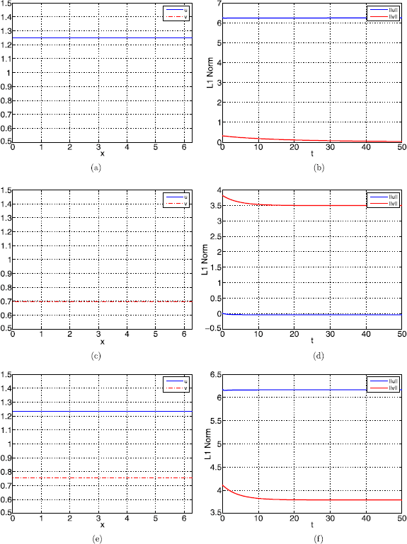
Numerical simulation of the stability for the constant equilibrium to (1.1): In (a) and (b), all the parameters are taken the same as those in Fig. 2(a) and (b); In (c) and (d), all the parameters are taken the same as those in Fig. 2(c) and (d); In (e) and (f), all the parameters are taken the same as those in Fig. 2 (e) and (f). Here, (a), (c) and (e) are the profiles of corresponding (a)–(b), (c)–(d) and (e)–(f) in Fig. 2 at time \(T=50\), the vertical axis in (b), (d) and (e) is the \(L_{1}\) norm of \(u\) or \(v\)
Fig. 4 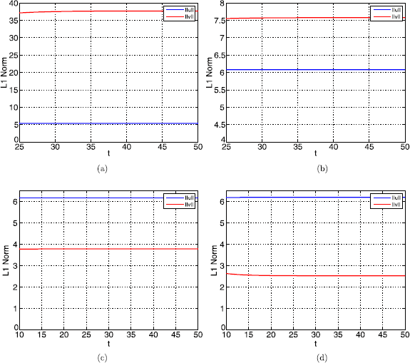
Effect of \(\beta\): The parameters \(a=1.25, \alpha=0.85\) and the same parameters as before except that \(\beta=0.1, 0.5, 1.0, 1.5\) for (a)–(d). The aim of plotting in the above domain is to explicitly show the change tendency of \(u\) and \(v\). Here, the initial conditions are \(u_{0}(x)=1+\cos(x), v_{0}(x)=1+\cos(x/2)\), the vertical axis is the \(L_{1}\) norm of \(u\) or \(v\)
-
(2)
If we use \(L^{1}\) norm \(\|u\|, \|v\|\) to represent the density \(u, v\), Fig. 4 show the effect of \(\beta\) on the density of prey and predator population. Noting that \(\beta\) is the strength of intraspecific interference, we take the parameters \(a=1.25, \alpha=0.85\) and the same parameters as before except that \(\beta=0.1, 0.5, 1.0, 1.5\) for Figs. 4(a)–(d), Fig. 4 presents a phenomenon that the population density of \(u\) is increasing as \(\beta\) increases, but the population density of \(v\) is in the opposite direction.


References
Beverton, R.J.H., Holt, S.J.: The theory of fishing. In: Graham, M. (ed.) Sea Fisheries; Their Investigation in the United Kingdom, pp. 372–441. Arnold, London (1956)
Crandall, M.G., Rabinowitz, P.H.: Bifurcation from simple eigenvalues. J. Funct. Anal. 8, 321–340 (1971)
De la Sen, M.: The generalized Beverton-Holt equation and the control of populations. Appl. Math. Model. 32(11), 2312–2328 (2008)
De la Sen, M., Alonso-Quesada, S.: Control issues for the Beverton-Holt equation in ecology by locally monitoring the environment carrying capacity: non-adaptive and adaptive cases. Appl. Math. Comput. 215(7), 2616–2633 (2009)
López-Gómez, J.: Spectral Theory and Nonlinear Functional Analysis. Research Notes in Mathematics, vol. 426. CRC Press, Boca Raton (2001)
López-Gómez, J., Molina-Meyer, M.: Bounded components of positive solutions of abstract fixed point equations: mushrooms, loops and isolas. J. Differ. Equ. 209(2), 416–441 (2005)
Liu, P., Shi, J., Wang, Y.: Imperfect transcritical and pitchfork bifurcations. J. Funct. Anal. 251(2), 573–600 (2007)
Lou, Y., Ni, W.M.: Diffusion, self-diffusion and cross-diffusion. J. Differ. Equ. 131(1), 79–131 (1996)
Pao, C.V.: Nonlinear Parabolic and Ellitic Equations. Plenum, New York (1992)
Pao, C.V.: Quasisolutions and global attractor of reaction-diffusion systems. Nonlinear Anal. 26(12), 1889–1903 (1996)
Potier-Ferry, M.: The linearization principle for the stability of solutions of quasilinear parabolic equations. I. Arch. Ration. Mech. Anal. 77(4), 301–320 (1981)
Smoller, J.: Shock Waves and Reaction-Diffusion Equations, 2nd edn. Springer, New York (1994)
Tang, S., Cheke, R.A., Xiao, Y.: Optimal impulsive harvesting on non-autonomous Beverton-Holt difference equations. Nonlinear Anal. 65(12), 2311–2341 (2006)
Yang, W., Wu, J., Nie, H.: Some uniqueness and multiplicity results for a predator-prey dynamics with a nonlinear growth rate. Commun. Pure Appl. Anal. 14(3), 1183–1204 (2015)
Yang, Z.P., Pao, C.V.: Positive solutions and dynamics of some reaction diffusion models in HIV transmission. Nonlinear Anal. 35(3), 323–341 (1999)
Author information
Authors and Affiliations
Corresponding author
Additional information
The work is supported by the Natural Science Foundation of China (No. 11501496) and the Special Fund of Education Department of Shaanxi Province (No. 16JK1710).
Rights and permissions
About this article

Cite this article
Yang, W. Existence and Asymptotic Behavior of Solutions for a Predator-Prey System with a Nonlinear Growth Rate. Acta Appl Math 152, 57–72 (2017). https://doi.org/10.1007/s10440-017-0111-8
Received:
Accepted:
Published:
Issue Date:
DOI: https://doi.org/10.1007/s10440-017-0111-8