
Abstract
This paper proposes a nonparametric approach with the purpose of estimating discrete wavelet transform (DWT) sub-band coefficients for high performance image interpolation. The number of clusters of defined statistical model that represents wavelet coefficients during the learning process is not fixed. The interpolating method is based on Hierarchical Dirichlet Process (HDP) where it uses the Blocked Gibbs Sampling method to obtain the optimum final values. The proposed HDP-HMM exploits statistical inter-scale, and intra-scale dependencies of image sub-bands of three-level decomposed 2D-DWT. It derives sub-bands of low resolution (LR) image, to obtain sub-bands of desired high resolution (HR) image. This research implements Hidden Markov model (HMM) to model the wavelet coefficients, and HDP to model the observations. It uses a very small size dataset that contains both LR and HR images of the dataset. The sophisticated statistical model introduced of the paper has excellent results in terms of Peak-to-Noise Ratio (PSNR), Structural Similarity Index (SSIM), Feature Similarity Index (FSIM), and Edge PSNR (EPSNR). It also has a great capability of repressing disturbing artifact, due to ability to model statistical dependencies of distant pixels. This method, and other compared state-of-the-art methods, have implemented on eighteen test-benches, with different statistical properties.
1 Introduction
Image interpolation is the resolution enhancement operation of a given low-resolution image, in order to magnify it to high-resolution image. The image interpolation problem can be observed from different standpoints. Wavelet domain image interpolation using various sub-band decomposition is a breakthrough. Wavelet theory has many applications in multiple areas of image processing. The dyadic multiresolution analysis (MRA) architecture for DWT which is presented by Mallat in 1989 [1] is the basic platform of this research.
It divides the frequency band into two reconstruction/ decomposition parts, and provides the ability to analyze the input signal by scale-two repeatedly, until the desired frequency resolution is achieved [1, 2]. Normally, in wavelet-based interpolation methods, the available LR image is assumed as the LL sub-band. By obtaining wavelet coefficients, the next finer scale image will be achieved. Changing the scale from LR to HR is the process of predicting lost high-frequency components of the image. Recent machine learning and data-driven approaches have improved the subjective quality of interpolated HR images. This category of approaches which includes neural network-based methods defines statistical chain models based on specific stochastic processes that fit the behavior of the corresponding data set [3]. We require to reduce image artifacts in order to achieve efficient estimation of pixel correlations. This paper concentrates on high efficiency estimation of sub-band coefficients using hidden Markov chains and nonparametric modeling by HDP.
DWT and DCT are two principal tools of image/video processing to manipulate, and enhance frequency band to achieve the desired intent. Therefore, in both algorithmic development and hardware implementation techniques, it has received a lot of attention from researchers [4,5,6]. The idea of image interpolation using Markov models based on DWT was for the first time offered in [7] and [8] researches. Locally adaptive zooming algorithm (LAZA) [9] uses adjustable thresholds to detect sharp edges and exploit data of discontinuous lines to update the interpolation process; however, the method still suffers from lack of accuracy in sharp lines. New edge-directed interpolation (NEDI) [10], and directional filtering and data fusion (DFDF) [11], are adaptive directional interpolants functioning while gaining image directional regularity but still having jaggies artifacts. The improved new edge-directed interpolation (INEDI) [12], has modified NEDI by using varying size training windows according to the edge size, and has obtained better results. Visual artifacts such as jaggies and ringing appear on INEDI. However, this method still has problem with jaggies on the edges. Xianming Liu et al. have proposed Interpolation via Graph-based Bayesian Label Propagation method (IGBLP), which is a graph-based method in which point labels propagate from known to unknown points of the graph based on Bayesian inference [13]. It performs based on Bayesian inference by labelling known and unknown pixels, the defined labels propagate from known to unknown points of the graph.
Seung-Jun et al. proposed an edge-guided method based on computing the derivatives and using Taylor series approximation and calculating intensity values of the desired pixels by an approximation of Taylor series [14]. This exploits information of sharp lines of image but still has problem of staircase effect in interpolating curvatures. Aguerrebere et al. also proposed a Bayesian approach method in which they use a Gaussian mixture model (GMM) to perform non-local patch-based restoration [15]. Abbas et al. proposed an adaptive interpolation algorithm which defines optimal values for trigonometric B-spline [16]. Khan et al. have proposed a low-complexity slope-based method that works based on Edge Slope Tracing (EST) that operates in a different way, in a way that, first, it predicts slope of the line that contains the intended pixel based on adjacent slopes. Then, it performs post-processing operations, in order to reduce artifacts, correct the edgy regions, and obtains the value of the intended pixel [17]. The interpolating algorithm presented in [18] has set a trade-off between performance and computational complexity of its achieved final results. This edge directed algorithm has used a gradient and edge map of the input image to interpolate unknown pixels in different predicted directions using known intensity pixels. It performs by classification of unknown pixels into obvious and transitional edges using a decision support system. The main struggle of these methods is their limited ability in finding correlation between distant pixels. Therefore, this research paper has proposed a sophisticated statistical model that operates in two directions in order to model and retrieve lost information as much as possible. This powerful model has remarkable capabilities in countering jaggies and disturbing artifacts. Its final PSNR, SSIM, FSIM results in most cases does better than mentioned competing methods. Section 2 explains the proposed method, the implementation process, and how it models inter-scale and intra-scale dependencies of the 2D-DWT to obtain a high performance image interpolation. Section 3 discusses the experimental results. The conclusion comes in Sect. 4.
2 Proposed interpolation method
-
A.
Problem definition
At the beginning, an appropriate dataset including both LR and HR images is presented. Then, as shown in Fig. 1, in order to exploit and study the statistical dependencies, Level 1, 2, and 3 sub-bands are extracted by three scale sub-band decomposition of each LR image. Then, through “tying” the coefficients of wavelet mother function to clusters of HDP-HMM, the model trains and obtains the optimum coefficient values achieve. The concept of tying coefficients to clusters, first time proposed by Crouse et al. [7].
Fig. 1. 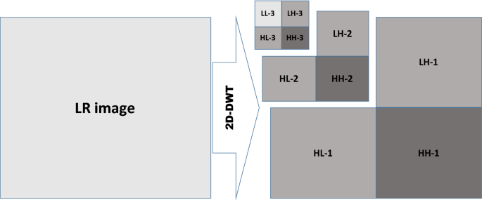
2D-DWT of LR image with sub-band decoding in three stages

Then, by obtaining wavelet coefficients from the statistical model in DWT domain, the input image will be decomposed one level, and level-1 sub-band is achieved. Eventually, through the proposed trans-band computation, three level-1 sub-bands of the input image will be doubled in size to three sub-band images of level-0. As shown in Fig. 2 by inverse 2D-DWT operation the intended output HR image is achieved. The detailed flowchart of the proposed method is shown in Fig. 3.

Generating HR image by Inv. 2D-DWT of LR and 0-level sub-bands

Detailed flowchart of the proposed algorithm
In order to derive coefficients of the desired mother function, HDP-HMM, as its name implies, it operates in two different phases. In the first phase, the behavior of coefficients within a specified MRA scale of DWT is modelled through hidden Markov chains. The intra-scale dependency extraction will describe in part B of this section. On the other hand, in second phase, the inter-scale dependencies between two levels of MRA are modelled by HDP. This includes statistical dependencies between level-1 and level-2, also between level-2 and level-3 of the LR images of dataset.
In machine learning, Dirichlet process (DP) has two important applications. Dirichlet Process Mixture Model (DPMM), and HDP. In the context of mixture model, a DP-distributed discrete random measure is used as a prior to the parameters of mixture components in a mixture model [19].
A DPMM mathematically is defined in terms of a base measure G0 and a concentration parameter α. The number of mixture components are not fixed, and this is why it is called infinite mixture model. In contrast, Gaussian mixture model (GMM) is a finite mixture model with prespecified components [20]. (1) describes DPMM in which θi = (µi, σi) of G is the mixture component parameters of the observed data, xi. Dist represents the distribution of mixture components [21].
HDP is the extended concept of DPMM. In order to link several mixture models (in the case of this research two mixture models), hierarchical Dirichlet process has been proposed [22, 23]. In fact, HDP allows to juxtapose prior observations of several groups of data with the same characteristics inside a model. This gives the ability of training based on defined combinatorial distribution for wavelet mother function.
-
B.
Intra-scale dependency extraction
Although in some researches wavelet coefficients have been assumed statistically independent, they could be modeled in several ways based on different distributions [24]. However, through studying the wavelet-function and scaling-function structure, we can demonstrate that their behavior can be modeled. Several statistical models which meet the statistical properties of natural images have been proposed for wavelet and scaling functions. For modeling and extracting intra-scale dependencies, this paper presumes two-state model as the basis for wavelet coefficient’s behavior [7, 8]. This idea is based on the fact that DWT wavelet function in the frequency domain could be shown with two hidden Markov chains. One of them for the marginal coefficients with small value (red), and the other for the central coefficients with large value (blue) as shown in Fig. 4. Its HMM block diagram is shown in Fig. 5
Fig. 4 
States of the Two-state model
Fig. 5 
Two-state model for wavelet function in frequency domain


Due to reconstructability principle of orthogonal DWT system, by mother function, the scaling functions can be achieved. Therefore, the purpose is to derive only the mother function from the proposed statistical model.
The final value is taken from one of the chains. Thus, the two are complementary and the sum of their probability density functions (pdf) is 1. \({P}_{s}\left({S}_{\mathrm{red}}\right)+{P}_{s}\left({S}_{\mathrm{blue}}\right)=1\). For the observed random variable W, the conditional pdf W|S should be obtained with respect to the red and blue states. Hence, the Gaussian pdf of W is as (2) which is how a coefficient wavelet associates itself with one of the aforementioned hidden Markov chains.
-
C.
Inter-scale dependency extraction
Like the case of intra-scale dependencies of particular level coefficients, statistical dependencies across DWT levels could also be modeled and extracted either. In order to obtain three sub-bands of level-0 that are the same size as the LR image, tracking the added frequency details in the three-level sub-band decomposition of the input image is required. In order to model inter-scale dependencies, a mixture model of Gaussians with the ability of varying the number of clusters has been used. With higher capabilities, a nonparametric hierarchical clustering model is suitable for HMM-based problems that are defined in a way that number of hidden states is not predefined [25].
HDP is assigned with one prior distribution, and two groups of data. As described in (3), G0 represents the base distribution of low-level mixture of DP prior. This distribution is drawn from the DP prior. Each drawn of GRed and GBlue from DP prior of DP(α0, G0) has a shared discrete base distribution [22].
Daub-8 filter-bank is an appropriate starting point. The function and hierarchical structure of an HDP could be seen in its block diagram that is shown in Fig. 6. In fact, each state itself could be considered to be a self-contained probabilistic model that consists of two chains of the two-state model shown in Fig. 5. Hidden states of the HMM correspond to the finer scale of DWT, and observed states correspond to the coarse scale, and HDP-HMM models statistical dependencies across wavelet scales.

The block diagram of HDP-HMM with two-state wavelet model
α: The concentration hyperparameter.
G0: The default value of G set for Daub-8 is NRED (9, 10) and NBLUE (9, 17).
Z: Observed state of the defined HMM.
X: Hidden state of the defined HMM.
-
D.
Function of HDP-HMM
The model receives an LR-HR set of each image dataset separately, and decomposes the LR image as explained. It takes the normalized wavelet coefficients of Daub-8 in the frequency domain as the starting point for training process, and ties them as initial values of the HMM hidden states [7]. The purpose of the training process is to get the highest PSNR value of the original and interpolated HR image for each sample. At each full cycle, in order to achieve this endpoint, the final post-training posterior probabilities are sampled 10,000 times by blocked Gibbs sampler. The algorithm takes the output as initial distribution for the next LR-HR set of dataset. Blocked Gibbs sampler will sample each clusters separately. Traditional DWT, HMM-based methods are trained using datasets with several hundreds of images [7, 26], but the proposed method has the capability to be trained with a very limited dataset, less than 30 images [5], [25] for the supervised HDP (sHDP).
The problem is considered by involving groups of data that each observation within a group is drawn from a mixture model, where it is desirable to share mixture components between groups. We assume that the number of mixture components is unknown at priori and will be inferred from the data [27]. The function of the two relating states of the model are explained here. The final number of clusters after optimization process is the final number of desired wavelet coefficients. Thus, we need to know the assignment of each data point to a cluster. Similar hierarchical Dirichlet processes are also used in text modeling applications such as [28] paper. That paper proposes a Nested HDP (nHDP) in which the hierarchy of Dirichlet processes are defined nested, where G as the base distribution of \(H\sim \mathrm{DP}(\alpha \text{,}G)\) is another DP with its own relating α, and base distribution\(G\sim \mathrm{DP}(\alpha \text{,J})\). In fact, each word follows its own path to a topic node, based on a document distribution on a specific tree that is modeled with a DP [29].
Sampling from conditional distribution is a task easier than sampling from marginal distributions for Gibbs sampler. The observation vector \(\mathop{z}\limits^{\rightharpoonup} = (z_{1}^{\left( n \right)} ,z_{2}^{\left( n \right)} , \ldots {,}z_{i}^{\left( n \right)} )\) is the objective assignment of each data point after n iteration. In order to update \({z}_{i}\) from the joint distribution\(P({{z}_{1}}\text{,}{{z}_{2}}\text{,}\dots \text{,}{{z}_{i}})\), by starting the clustering and data assignment process, let’s assume each data point of observations is dependent on clustering of its neighboring clusters. As shown in (4), the process unfolds with the general presumption that data depends on clusters and parameters before narrowing down the cluster dependencies.
\({z}_{i}\): Observed and assigned data to ith cluster.
\({z}_{-i}\): Data related to all z parameters, except \({z}_{i}\).
\({x}_{\mathrm{i}}\): The data associated with the ith cluster.
\(\mathop{x}\limits^{\rightharpoonup}\): Observation input of Dataset.
\({\theta }_{k}\): Parameters associated to cluster k.
α: The concentration hyperparameter.
G: The base distribution of two-state HMM.
Each data point depends on the clustering of its neighbors, and the probability distribution parameters. Therefore, \(P\left({z}_{i}|{z}_{-i}\right)\) can be written as (5).
Let’s take a random guess initially by cluster assignment of each observation which provides a mean for each cluster. Based on weights of atoms, clusters either grow or shrink. Therefore, by updating \({z}_{i}\) and incrementally changing all the assignments, after a chain of observations, we will find that they correct themselves. This is necessary to obtain the sequence of observations, which is derived by expanding, and specifying the equation. By applying chain rule we reach to (6). The mean of the data is related to \({x}_{i}\) of the particular cluster belongs to. In other words, in terms of the DPMM problem presentation of Chinese restaurant process, it is equivalent to what table we are sitting at.
The observation associated with the mean of a cluster and \({\mathrm{x}}_{\mathrm{i}}\), the data associated with the cluster are conditioned to input data [30]. Given the mean and covariance matrix of cluster k, by separating their conditional probabilities, respectively, for both cases with and without added clusters we get (7) and (8) for \(P\left( {z_{i} |z_{ - i} } \right)\).
By calculation of integrals, (9) and (10) are obtained from (7) and (8). It turns out that clusters are assigned with a normal distribution.
\(n\): Total data.
\({n}_{\overline{x} }\): The mean of data.
\({n}_{k}\): Categorized data in clusters.
During the optimization process, by obtaining the optimized values of conditional probabilities, the posterior distributions are sampled 10,000 times for each cycle. This is performed by Blocked Gibbs sampling that operates separately for each cluster. The final number of clusters and their mean values are the numbers of wavelet coefficients and their value. Due to wavelet function’s symmetric nature after posterior distributions of clusters of a nonparametric Bayesian mixture model, each sampling operation comes with symmetricizing operation of the coefficients. Meanwhile, the final number of HMM states that represents and embodies the DWT coefficients, is determined by the training process. Due to the clustering property of the DP, some data points will share the same parameters θ, which can be represented as those data points being assigned to the same topic.
-
E.
Trans-band computation
After wavelet function generation, and subsequent scaling function generation from the model, in order to obtain level-0 sub-bands (sub-bands of HR image), a trans-band computation has introduced. Trans-band computation follows the pattern of changes in three level-1, level-2, and level-3 sub-bands that were generated by derived filter banks, and extend it to level-0 sub-band. The general idea behind this section is related to the usual pattern of filtered sub-bands (Fig. 7).

General pattern of 2D-DWT sub-bands of a natural image a LH in up-right b HL in down-left c HH in down-right
LH Sub-band: Generally, the LH sub-band filtered by LPF row-wise, and by HPF column-wise, are continuous row-wise peaks with two-sided slopes toward top and bottom of the sub-band (as shown in Fig. 7a). As shown in Fig. 8, \({x}_{m/2\text{,}n/2}^{3}\) and \({x}_{m/2-1\text{,}n/2}^{3}\) are pixels of a single column in LH-3 sub-band. By moving toward LH-2 sub-band, it vertically transforms to rectangular eight pixels, and in one step further it obtains the corresponding thirty-two pixels of LH-1 sub-band. Column-wise for LH sub-band a Curve-fitting algorithm aimed at maintaining the curvature of the hillsides is the basis of the work. Curve-fitting and filling the blank pixels with best value, is a suitable choice in this case, and exploits the provided platform in best way. The convexity of the changes is the determining factor in filling blank pixels while moving to the next level-0 sub-band. Row-wise, cubic spline is implemented.

Moving from LH-3 to LH-2 and LH-1 sub-bands
HL Sub-band: In the case of HL sub-band Trans-band computation acts in an opposite manner which means that row-wise curve-fitting and column-wise cubic spline are implemented (as shown in Fig. 7b).
HH Sub-band: Regarding HH sub-band, in both dimensions, cubic spline is implemented, in order to obtain HH-0 sub-band.
By obtaining LH-0, HL-0, and HH-0 sub-bands, and taking the LR image as the LL-0 sub-band image, we are able to operate a 2D-IDWT and obtain the desired HR image as shown in Fig. 9. The similar but row-wise pattern is correct for HL-1 sub-band.

Building HL-0, LH-0, and HH-0 sub-bands and deriving HR image by inverse 2D-DWT
3 Experimental results
The proposed algorithm is applied to eighteen mostly-used standard test-images with completely different sizes, and statistical properties that can prove an interpolating algorithm’s efficiency (Table 1). Test images are obtained from [31, 32], and [33].
Experimental results are presented to demonstrate the performance of the proposed algorithm. They have compared against the twelve most prominent, and the latest interpolating algorithms. Since the results of all eighteen test-benches are not available in each mentioned papers, they are reproduced in this research, and the results have matched with the existing results in the original papers. Proposed algorithm in PSNR, and FSIM outperforms in eleven test-benches, and in SSIM outperforms in ten test-benches.
Comparison results are presented in PSNR, SSIM, and FSIM in Table 2. Peak signal-to-noise ratio is a subjective method as the most common criterion to measure the quality of the output image in all image processing applications. It is the maximum power of the signal to the power of distorting noise ratio. SSIM is an image similarity test based on the structure of the image that looks at the issue from different angle [34]. It is an objective method to assess the differences between output image and the reference image based on their averages, variances, and covariance calculations. Furthermore, this research paper has conducted the subjective evaluation of the final results from a different perspective. FSIM is the extended concept of SSIM. Like SSIM, the basis of this criterion for quality assessment is to bring pixel-based analysis to structure-based [35]. FSIM operates based on the fact that human visual system (HVS) understands an image mainly according to its low-level features. The primary feature of SSIM is phase congruency (PC), which is a dimensionless measure of the significance of a local structure. The secondary feature of FSIM is the image’s gradient magnitude (GM) that encodes contrast information of the target image [36].
Moreover, for the reader’s further study of algorithm’s performance in the sub-bands, this survey has conducted an EPSNR comparison. Here, Sobel filter is used to distinguish the edges of the original HR image, and the PSNR of the pixels on the edge are used to generate the EPSNR [39]. This is a very good evaluation of image sub-bands, and how their edges, and slopes are predicted, and built in different directions before Inverse 2D-DWT, after Trans-band computation. Table 3 presents the EPSNR results of the proposed and the competing results. The Table has presented EPSNR values of the three LH-0, HL-0, and HH-0 sub-bands. The proposed algorithm in HL-band EPSNR, and HH-band EPSNR outperforms in twelve test-benches, and in LH-band EPSNR outperforms in eleven test-benches.
Table 4 gives the complexity comparison of the proposed and twelve competing methods on eighteen test benches. MATLAB 2018 is the used IDE which is run by a typical laptop (Intel Corei3 CPU 2.00 GHZ, 1G memory RAM). As discussed in previous section, the filter-bank coefficients of the proposed HDP-HMM, and DWT-based method have the ability to be trained using a very small dataset down to 30 images. In this experiment, in order to observe this process, five image galleries, Ga. 1, Ga. 2, Ga. 3, Ga. 4, and Ga. 5 with 10, 20, 30, 40, 50 LR-HR set of images have been tested. The dataset for each image can be provided online easily, and for algorithm’s similar input images like Pepper, and Fruit, the same dataset is used. The complexity of time is related to the size of the image. For example, for the large images of the Kodiak database like Airplane, and Splash it takes longer, whereas for smaller images like Cameraman, Arial, and Clock, the time is shorter. Also it is important to note that, original input samples should not be used for the test. In order to investigate the effect of dataset size on the quality of the output images in Table 5, each gallery was tested five times using different images then we averaged their final values. As can be seen in that table, 30-size datasets are sufficient for this experiment. Table 6 presents the learning time of the statistical model for each image gallery of each test bench.
Finally, to view the performance of the model and the objective quality of the interpolated images, two test images are chosen. Lena, and Baboon are considered as highly and lowly correlated images in papers. Figures 10, and 11 show the considered Ga. 1 to Ga. 5 datasets. Figures 12, and 13 show the interpolated results with four highlighted regions. By scrutinizing the critical locations of the two images such as Lena's eye, and eyebrow, and Baboon's nose, and mustaches, it is clear that the method’s ability to suppress jaggies and disturbing artifacts is outstanding. This is the result of taking advantage of the inter-scale and intra-scale dependencies of the image sub-bands.

Lena’s dataset for Gallery 1 to gallery 5

Baboon’s dataset for Gallery 1 to gallery 5

Interpolated ‘Lena’ with 4 highlighted regions, and used dataset

Interpolated ‘Baboon’ with 4 highlighted regions, and used dataset
4 Conclusion
This paper proposes a sophisticated probabilistic model for HDP-HMM based image interpolation. It decomposes the input LR image, models the wavelet coefficients and exploits the inter-scale statistical dependencies of three consecutive sub-bands and intra-scale statistical dependencies of obtained wavelet function. HMM is the platform for modeling wavelet coefficients, and HDP models the observation. It uses Dirichlet distributions as prior distributions in Bayesian statistics, for clustering analysis and statistical data clustering.
During the learning process, the statistical model divides the data population into subpopulations that fit our model without constraining continuity over the entire model we used to encounter before. Through optimization of filter-banks by this nonparametric statistical tool, we have achieved better results than most of the state-of-the-art image interpolating methods. This is the result of the statistical model’s ability to exploit statistical dependencies of distant pixels. As a result of taking great advantage of statistical dependencies, the output interpolated images of the HDP-HMM has a great ability in suppressing jaggies and ringing artifact.
References
Mallat S (1989) A theory for multiresolution signal decomposition: the Wavelet representation. IEEE Trans Patt Anal Mach 11(7):674–693
Guoshen Yu, Sapiro G, Mallat S (2012) Solving inverse problems with piecewise linear estimators: from Gaussian mixture models to structured sparsity. IEEE Trans Image Proc 21(5):2481–2499
Plaziac N (1999) Image interpolation using neural networks. IEEE Trans Image Proc 8(11):1647–1651
Sarkar S, Bhairannawar SS (2021) Efficient FPGA architecture of optimized Haar wavelet transform for image and video processing applications. Multidimens Syst Signal Process. 32:821–844
Ibraheem MS, Hachicha K, Ahmed SZ, Lambert L, Garda P (2019) : High-throughput parallel DWT hardware architecture implemented on an FPGA-based platform. J Real-Time Image Proc 16:2043–2057
AbdolVahab Khalili Sadaghiani, M. Ghanbari: An Optimized Hardware Design for high speed 2D-DCT processor based on modified Loeffler architecture. In: 27th Iranian Conference on Electrical Engineering (ICEE), pp. 1476–1480. (2019).
Crouse MS, Nowak RD, Baraniuk RG (1998) Wavelet-based signal processing using hidden markov models. IEEE Trans Signal Proc 6(4):886–902
K Kinebuchi, DD Muresan, TW Parks (2001) Image interpolation using wavelet based hidden Markov trees. In: International Conference on Acoustics, Speech, and Signal Processing. In: Proceedings , Salt Lake City, Utah May, pp. 7–11.
Battiato S, Gallo G, Stanco F (2002) A locally-adaptive zooming algorithm for digital images. Image Vis Comput 20(11):805–812
Li X, Orchard MT (2001) New edge-directed interpolation. IEEE Trans on Image Proc 10:1521–1527
Zhang L, Wu X (2002) Image interpolation via directional filtering and data fusion. IEEE Trans Image Process 15(8):2226–2238
N Asuni and A Giachetti: Accuracy improvements and artifacts removal in edge based image interpolation. In: International Joint Conference on Computer Vision, Imaging and Computer Graphics Theory and Application, (2008).
Liu X, Zhao D, Zhou J, Gao W, Sun H (2014) Image Interpolation via graph-based bayesian label propagation. IEEE Trans image process 23(3):1084–1096
Lee S-J, Kang M-C, Uhm K-H, Ko S-J (2016) An edge-guided image interpolation method using taylor series approximation. IEEE Trans Consumer Electron 62(2):159–165
Aguerrebere C, Almansa A, Delon J, Gousseau Y, Mus P (2017) A bayesian hyperprior approach for joint image denoising and interpolation, with an application to HDR imaging. IEEE Trans Comput Imag 3(4):633–646
Abbas S, Irshad M (2018) Malik Zawwar Hussain: Adaptive image interpolation technique based on cubic trigonometric B-spline representation. IET Image Proc 12(5):769–777
Khan S, Lee D-h, Khan MA, Gilal AR, Mujtaba G (2019) Efficient edge-based image interpolation method using neighboring slope information. IEEE Access 7:133539–133548
Khan S, Lee DH, Khan MA, Siddiqui MF, Zafar RF, Memon KH, Mujtaba G (2020) Image interpolation via gradient correlation-based edge direction estimation. Sci Program 2020:1–12
Orhan AE, Jacobs RA (2013) A probabilistic clustering theory of the organization of visual short-term memory. Psychol Rev 120(2):297
Rasmussen CE The Infinite Gaussian Mixture Model. In: Proceedings of the 12th International Conference on Neural Information Processing Systems, Denvor, CO, USA, 554–560 (1999).
Gorur D, Rasmussen CE (2010) Dirichlet process gaussian mixture models, choice of the base distribution. J Comp Sci Technol 25(4):615–626
S Mohamad, A Bouchachia, and MS Mouchaweh A Non-parametric Hierarchical Clustering Model. In: International Conference on Evolving and Adaptive Intelligent Systems (EAIS), Douai, France, (2015).
Neal RM (2000) Markov chain sampling methods for dirichlet process mixture models. J Comput Graph Stat 9(2):249–265
H Choi, RG Baraniuk (1999) Image segmentation using wavelet domain classification. In: Mathematical modeling, bayesian estimation, and inverse problems, international society for optics and photonics, vol 3816, pp 306–320
DB DAHL (2006) Model-based clustering for expression data via a dirichlet process mixture model. In: Bayesian inference for gene expression and proteomics, chap 10. Blackwell, London, pp 201–218
AK Sadaghiani, S Sheilkhai, B Forouzandeh High Performance Image Compression Based on Optimized EZW Using Hidden Markov Chain and Gaussian Mixture Model. In: 28th Iranian Conference on Electrical Engineering (ICEE), pp. 1–5. (2020).
Rabiner L (1989) A tutorial on hidden Markov models and selected applications in speech recognition. Proc IEEE 77(2):257–286
Teh YW, Joedan Ml, beal MJ, Blei DM (2012) Hierarchical Dirichlet processes. J Am Stat Assoc 101(476):1566–1581
Chien J-T (2017) Bayesian nonparametric learning for hierarchical and sparse topics. IEEE Trans Audio Speech Language Process 26(2):422–435
Mahalakshmi GS, MuthuSelvi G, Sendhilkumar S (2019) Gibbs sampled hierarchical Dirichlet mixture model based approach for clustering scientific articles. Smart Comput Parad New Progresses Challenges 766:169–177
Zhang L, Zhang L, Mou X, Zhang D (2011) FSIM: a feature similarity index for image quality assessment. IEEE Trans Image Process 20(8):2378–2386
Bagheri E, Dastghaibyfard G, Hamzeh A (2018) FSIM: a fast and scalable influence maximization algorithm based on community detection. Int J Uncertain Fuzziness Knowl Based Syst 26(3):379–396
Maksimović-Moićević S, Lukač Ž, Temerinac M (2019) Objective estimation of subjective image quality assessment using multi-parameter prediction. IET Image Process 13(13):2428–2435
A. Giachetti and N. Asuni: Fast artifacts-free image interpolation. In: British Machine Vision Conference, (2008).
Liu X, Zhao D, Xiong R, Ma S, Gao W, Sun H (2011) Image interpolation via regularized local linear regression. IEEE Trans on Image Process 20(12):3455–3469
Zhou W, Bovik AC, Sheikh HR, Simoncelli EP (2004) Image quality assessment: from error visibility to structural similarity. IEEE Trans Image Process 13(4):600–612
Author information
Authors and Affiliations
Corresponding authors
Additional information
Publisher's Note
Springer Nature remains neutral with regard to jurisdictional claims in published maps and institutional affiliations.
Rights and permissions
About this article

Cite this article
Khalili Sadaghiani, A., Forouzandeh, B. Image interpolation based on 2D-DWT and HDP-HMM. Pattern Anal Applic 25, 361–377 (2022). https://doi.org/10.1007/s10044-022-01057-4
Received:
Accepted:
Published:
Issue Date:
DOI: https://doi.org/10.1007/s10044-022-01057-4