Analysis of multipatch discontinuous Galerkin IgA approximations to elliptic boundary value problems

Abstract

In this work, we study the approximation properties of multipatch dG-IgA methods, that apply the multipatch Isogeometric Analysis discretization concept and the discontinuous Galerkin technique on the interfaces between the patches, for solving linear diffusion problems with diffusion coefficients that may be discontinuous across the patch interfaces. The computational domain is divided into non-overlapping subdomains, called patches in IgA, where B-splines, or NURBS approximations spaces are constructed. The solution of the problem is approximated in every subdomain without imposing any matching grid conditions and without any continuity requirements for the discrete solution across the interfaces. Numerical fluxes with interior penalty jump terms are applied in order to treat the discontinuities of the discrete solution on the interfaces. We provide a rigorous a priori discretization error analysis for diffusion problems in two- and three-dimensional domains, where solutions patchwise belong to $W^{l,p}$, with some $l\ge 2$ and $p\in ({2d}/{(d+2(l-1))},2]$. In any case, we show optimal convergence rates of the discretization with respect to the dG - norm.

1 Introduction

The finite element methods (FEM) and, in particular, discontinuous Galerkin (dG) finite element methods are very often used for solving elliptic boundary value problems which arise from engineering applications, see, e.g., [17] and [25]. For realistic problems in complicated geometries, the quality of the numerical results depends usually on the quality of the discretized geometry (triangulation of the domain), which is usually performed by a mesh generator. This is the case even if curved elements are used, see, e.g., [8, 22, 36] and [17]. In many practical situations, extremely fine meshes are required around fine-scale geometrical objects, singular corner points etc. in order to achieve numerical solutions with desired resolution. This fact leads to an increased number of degrees of freedom, and thus to an increased overall computational cost for solving the discrete problem, see, e.g., [32] for fluid dynamics applications.

Recently, the Isogeometric Analysis (IgA) concept has been applied for approximating solutions of elliptic problems [5, 18]. IgA generalizes and improves the classical FE (even isoparametric FE) methodology in the following direction: complex technical computational domains can be exactly represented as images of some parameter domain, where the mappings are constructed by using superior classes of basis functions like B-spline, or Non-Uniform Rational B-spine(NURBS), see, e.g., [9] and [28]. The same class of functions is used to approximate the exact solution without increasing the computational cost for the computation of the resulting stiffness matrices [9], systematic hpk refinement procedures can easily be developed [33], and, last but not least, the method can be materialized in parallel environment incorporating fast domain decomposition solvers [20], [34], [2].

During the last two decades, there has been an increasing interest in discontinuous Galerkin (dG) finite element methods for the numerical solution of several types of partial differential equations, which is attributed to the advantages of the local approximation spaces without continuity requirements that dG methods offer, see, e.g., [3, 10, 27, 29] and [31].

In this paper, we combine the best features of the two aforementioned methods, and develop a discretization method that we call multipatch discontinuous Galerkin Isogeometric Analysis (dG-IgA). We apply and analyze the proposed dG-IgA method to elliptic boundary value problems with discontinuous coefficients. It well known that the solutions of this type of problems are in general not smooth enough, see, e.g. [19, 21], and the numerical method cannot produce an (optimal) accurate solution. The problem is set in a complex, bounded Lipschitz domain $\varOmega \subset \mathbb {R}^d, d=2,3$, which is subdivided in a union of non-overlapping subdomains, say $\mathcal{{S}}(\varOmega ):=\{\varOmega _i\}_{i=1}^N$, where we further assume that the discontinuity of the diffusion coefficients is only observed across the subdomain boundaries (interfaces). The weak solution of the problem is approximated in every subdomain applying IgA methodology, [5], without imposing continuity requirements for the approximation spaces across the interfaces. Having in our mind more general problems, where the use of independent subdomain meshes is more preferable, see, for example, [4] for the use of dG techniques in the case of rotating subdomains, we develop our numerical analysis for non-matching meshes across the interfaces. By construction, dG methods use discontinuous approximation spaces utilizing numerical fluxes on the interfaces, [3], and have been efficiently used for solving problems on non-matching grids in the past, [10, 11, 14]. Here, emulating the dG finite element methods, the numerical scheme is formulated by applying numerical fluxes with interior penalty coefficients on the interfaces of the subdomains (patches), and using IgA formulations in every patch independently. A crucial point in the presented work, is the expression of the numerical flux interface terms as a sum over the micro-elements edges taking note of the non-matching subdomain meshes. This gives the opportunity to proceed in the error analysis by applying the trace inequalities locally as in dG finite element methods. There are many papers, which present dG finite element approximations for elliptic problems, see, e.g., [3], the monographs [27, 29], and, in particular, for the discontinuous coefficient case, [10, 26]. However, there are only a few publications on the dG-IgA and their analysis. In [7], the author presented discretization error estimates for the dG-IgA of plane (2d) diffusion problems on meshes matching across the patch boundaries and under the assumption of sufficiently smooth solutions. This analysis obviously carries over to plane linear elasticity problems which have recently been studied numerically in [2]. In [12], the dG technology has been used to handle no-slip boundary conditions and multipatch geometries for IgA of Darcy-Stokes-Brinkman equations. DG-IgA discretizations of heterogeneous diffusion problems on open and closed surfaces, which are given by a multipatch NURBS representation, are constructed and rigorously analyzed in [24].

In the first part of this paper, we give a priori error estimates in the dG-norm $\Vert .\Vert _{dG}$ under the usual regularity assumption imposed on the exact solution, i.e. $u\in W^{1,2}(\varOmega )\cap W^{l\ge 2,2}(\mathcal{{S}}(\varOmega ))$. Next, we consider the model problem with low regularity solution $u\in W^{1,2}(\varOmega )\cap W^{l,p}(\mathcal{{S}}(\varOmega ))$, with $l\ge 2$ and $p \in (\frac{2d}{d+2(l-1)},2)$, and derive error estimates in the dG-norm $\Vert .\Vert _{dG}$. These estimates are optimal with respect to the space size discretization. We note that the error analysis in the case of low regularity solutions includes many ingredients of the dG FE error analysis presented in [35] and [26]. To the best of our knowledge, optimal error analysis for IgA discretizations combined with dG techniques for solving elliptic problems with discontinuous coefficients in general domains $\varOmega \subset \mathbb {R}^d$, $d=2,3$, have not been yet presented in the literature.

The paper is organized as follows. In Section 2, our model diffusion problem is described. Section 3 introduces some notations. The local approximation spaces $\mathbb {B}_h(\mathcal{{S}}(\varOmega ))$ and the numerical scheme are also presented in this section. Several auxiliary results and the analysis of the method for the case of sufficiently regular solutions are provided in Section 4. Section 5 is devoted to the analysis of the method for low regularity solutions. Section 6 includes several numerical examples that verify the theoretical convergence rates. Finally, we draw some conclusions.

2 The model problem

Let $\varOmega$ be a bounded Lipschitz domain in $\mathbb {R}^d,{\ }d=2,3$, with the boundary $\partial \varOmega$. For simplicity, we restrict our study to the model diffusion problem

$$\begin{aligned} -\mathrm {div}(\alpha \nabla u) = {f}{\ } \text {in}{\ } \varOmega , {\ } \text {and}{\ }{u} = {u}_D {\ }\text {on } \partial \varOmega , \end{aligned}$$

(2.1)

where f and $u_D$ are given smooth data. In (2.1), $\alpha$ is the diffusion coefficient that is assumed to be bounded by strictly positive constants from above and below. Moreover, for the sake of simplicity, we will later assume that $\alpha$ is patchwise constant.

The weak formulation is to find a function $u\in W^{1,2}(\varOmega )$ such that $u:=u_D$ on $\partial \varOmega$ and satisfies

$$\begin{aligned} a(u,\phi )= l(\phi ),{\ } \forall \phi \in W^{1,2}_{0}(\varOmega ), \end{aligned}$$

(2.2a)

where

$$\begin{aligned} a(u,\phi )= \int _{\varOmega }\alpha \nabla u\nabla \phi \,dx, \quad \text {and}\quad l(\phi )=\int _{\varOmega }f\phi \,dx. \end{aligned}$$

(2.2b)

Results concerning the existence and uniqueness of the solution u of problem (2.2) can be derived by a simple application of Lax-Milgram Lemma, [13]. To avoid unnecessary long formulas below, we only considered in (2.1) non-homogeneous Dirichlet boundary conditions on $\partial \varOmega$. However, the analysis can be easily generalized to Neumann and Robin type boundary conditions on a part of $\partial \varOmega$, since they are naturally introduced in the dG formulation.

3 Preliminaries - dG notation

Throughout this work, we denote by $L^p(\varOmega ), p>1$ the Lebesgue spaces for which $\int _{\varOmega }|u(x)|^p\,dx < \infty$, endowed with the norm $\Vert u\Vert _{L^p(\varOmega )} = \big (\int _{\varOmega }|u(x)|^p\,dx\big )^{\frac{1}{p}}$. By $\mathcal {D}(\varOmega )$, we define the space of $C^{\infty }$ functions with compact support in $\varOmega$, and by $C^{k}(\varOmega )$ the set of functions with $k-th$ order continues derivatives. In dealing with differential operators in Sobolev spaces, we use the following common conventions. For any (multi-index) $\alpha =(\alpha _1,\ldots ,\alpha _d), {\ }\alpha _j\ge 0, j=1,\ldots ,d$, with degree $|\alpha | = \sum _{j=1}^d\alpha _j$, we define the differential operator

$$\begin{aligned} D^a=D_1^{\alpha _1}\cdots D_d^{\alpha _d},\text {with} {\ }D_j=\frac{\partial }{\partial x_j}, D^{(0,\ldots ,0)}u=u. \end{aligned}$$

(3.1)

We also denote by $W^{l,p}(\varOmega )$, l positive integer and $1\le p \le \infty$, the Sobolev space functions endowed with the norm

$$\begin{aligned} \Vert u\Vert _{W^{l,p}(\varOmega )}&= \big (\sum _{0\le |\alpha | \le m} \Vert D^{\alpha }u\Vert _{L^p(\varOmega )}^p\big )^{\frac{1}{p}},{\ } \Vert u\Vert _{W^{l,\infty }(\varOmega )} \nonumber \\&= \max _{0\le |\alpha | \le m} \Vert D^{\alpha }u\Vert _{\infty }. \end{aligned}$$

(3.2a)

For more details for the above definitions, we refer [1]. In the sequel we write $a\sim b$ if $c a \le b \le C a$, where c, C are positive constants independent of the mesh size.

In order to apply the IgA methodology for the problem (2.1), the domain $\varOmega$ is subdivided into a union of subdomains $\mathcal{{S}}(\varOmega ):=\{\varOmega _i\}_{i=1}^{N}$, such that

$$\begin{aligned} \bar{\varOmega }&= \bigcup _{i=1}^N \bar{\varOmega }_i,\quad \text {with}\quad \varOmega _i\cap \varOmega _j = \emptyset {}, {\ } \text {if}{\ }j\ne i. \end{aligned}$$

(3.3)

Throughout the paper we assume that the coefficient $\alpha$ in (2.1) is equal to some given positive constant $\alpha ^{(i)}$ in each subdomain $\varOmega _i$ for $i=1,\ldots ,N$.

As it is common in the IgA analysis, we assume a parametric domain $\widehat{D}$ of unit length, (e.g. $\widehat{D} = [0,1]^d$). For any $\varOmega _i$, we associate $n=1,\ldots ,d$ knot vectors $\varXi ^{(i)}_n$ on $\widehat{D}$, which create a mesh $T^{(i)}_{h_i,\widehat{D}} =\{\hat{E}_{m}\}_{m=1}^{M_i}$, where $\hat{E}_{m}$ are the micro-elements, see details in [9]. We shall refer $T^{(i)}_{h_i,\widehat{D}}$ as the parametric mesh of $\varOmega _i$. For every $\hat{E}_m\in T^{(i)}_{h_i,\widehat{D}}$ we denote by $h_{\hat{E}_m}$ its diameter and by $h_i=\max \{h_{\hat{E}_m}\}$ the meshsize of $T^{(i)}_{h_i,\widehat{D}}$. We assume the following quasi-uniformity properties for every $T^{(i)}_{h_i,\widehat{D}}$: (i) for every $\hat{E}_m\in T^{(i)}_{h_i,\widehat{D}}$ holds ${h}_i\sim h_{\hat{E}_m}$, (ii) for the micro-element edges $e_{\hat{E}_m} \subset \partial \hat{E}_m$ holds $h_{\hat{E}_m} \sim e_{\hat{E}_m}$.

On every $T^{(i)}_{h_i,\widehat{D}}$, we construct the finite dimensional space $\hat{\mathbb {B}}^{(i)}_{h_i}$ spanned by B-spline basis functions of degree k, [9, 30],

$$\begin{aligned} \hat{\mathbb {B}}^{(i)}_{h_i}= span\{\hat{B}_j^{(i)}(\hat{x})\}_{j=0}^{dim(\hat{\mathbb {B}}_{h_{i}}^{(i)})}, \end{aligned}$$

(3.4a)

where every $\hat{B}_j^{(i)}(\hat{x})$ base function in (3.4a) is derived by means of tensor products of one-dimensional $\mathbb {B}$-spline basis functions, e.g.

$$\begin{aligned} \hat{B}_j^{(i)}(\hat{x}) = \hat{B}_{j_1}^{(i)}(\hat{x}_1)\cdots \hat{B}_{j_d}^{(i)}(\hat{x}_d). \end{aligned}$$

(3.4b)

For simplicity, we assume that the basis functions of every $\hat{\mathbb {B}}_{h_{i}}^{(i)}, i=1,\ldots ,N$ are of the same degree k. We denote by $\tilde{D}^{(i)}_{\hat{E}}$ the support extension of $\hat{E}\in T^{(i)}_{h_i,\widehat{D}}$.

Every subdomain $\varOmega _i\in \mathcal{{S}}(\varOmega ), i=1,\ldots , N$, is exactly represented through a parametrization (one-to-one mapping), [9], having the form

$$\begin{aligned} {\varvec{\Phi }}_i: \widehat{D} \rightarrow \varOmega _i,&\quad {\varvec{\Phi }}_i(\hat{x}) = \sum _{j}C^{(i)}_j \hat{B}_j^{(i)}(\hat{x}):=x\in \varOmega _i, \end{aligned}$$

(3.5a)

$$\begin{aligned} \text {with}&\quad \hat{x} = {\varvec{\Psi }}_i(x):={\varvec{\Phi }}^{-1}_i(x), \end{aligned}$$

(3.5b)

where $C_j^{(i)}$ are the control points. For the purposes of this work, we assume that the components ${\varvec{\Psi }}_i=(\varPsi _{i,1},\ldots ,\varPsi _{i,d})$ and ${\varvec{\Phi }}_i=(\varPhi _{i,1},\ldots ,\varPhi _{i,d})$ are highly smooth functions.

Using ${\varvec{\Phi }}_i$, we construct a mesh $T^{(i)}_{h_i,\varOmega _i} =\{E_{m}\}_{m=1}^{M_i}$ for every $\varOmega _i$, whose vertices are the images of the vertices of the corresponding mesh $T^{(i)}_{h_i,\widehat{D}}$ through ${\varvec{\Phi }}_i$. If $h_{\varOmega _i}=\max \{h_{E_m}\}, {\ }E_m\in T^{(i)}_{h_i,\varOmega _i}$ is the subdomain $\varOmega _i$ mesh size, then based on Definition (3.5) of ${\varvec{\Phi }}_i$, there is a constant $C:=C(\Vert {\varvec{\Phi }}_i\Vert _{\infty })$ such that $h_i \sim C h_{\varOmega _i}.$ In what follows, we denote the subdomain mesh size by $h_i$ without the constant $C:=C(\Vert {\varvec{\Phi }}_i\Vert _{\infty })$ explicitly appearing.

The mesh of $\varOmega$ is considered to be $T_h(\varOmega )=\bigcup _{i=1}^N T^{(i)}_{h_i,\varOmega _i}$, where we note that there are no matching mesh requirements on the interior interfaces $\partial \varOmega _i \bigcap \partial \varOmega _j, i\ne j$.

For the sake of brevity in our notations, the interior faces of $\varOmega _i$ which are common to the interior faces of $\varOmega _j$ are denoted by $F_{ij}$, i.e., $F_{ij}= \partial \varOmega _i \cap \partial \varOmega _j,\,i\ne j$. We denote the collection of the faces that belong to $\partial \varOmega _i \cap \partial \varOmega$ by $\mathcal {F}_{i,B}$.

Lastly, we define on $\varOmega$ the finite dimensional $\mathbb {B}-$spline space

$\mathbb {B}_h(\mathcal{{S}}(\varOmega ))=\mathbb {B}^{(1)}_{h_{1}}\times ... \times \mathbb {B}^{(N)}_{h_{N}}$, where every $\mathbb {B}^{(i)}_{h_{i}}$ is defined on $T^{(i)}_{h_i,\varOmega _i}$ as follows

$$\begin{aligned} \mathbb {B}^{(i)}_{h_{i}}:=\{B_{h_{i}}^{(i)}|_{\varOmega _i}: B_h^{(i)}({x})= \hat{B}_h^{(i)}\circ {\varvec{\Psi }}_i({x}),{\ } \forall \hat{B}_h^{(i)}\in \hat{\mathbb {B}}^{(i)}_{h_i} \}. \end{aligned}$$

(3.6)

We define the union support in physical subdomain $\varOmega _i$ as $D^{(i)}_{E}:={\varvec{\Phi }}(\tilde{D}^{(i)}_{\hat{E}})$.

Assumption 1

We suppose that there exist constants $0<c_m<c_M$ such that for all $\hat{x}\in \hat{D}$

$$\begin{aligned} c_m \le |det({\varvec{\Phi }}^{'}_{i}(\hat{x}))| \le c_M, {\ }i=1,\ldots ,N, \end{aligned}$$

(3.7)

where ${\varvec{\Phi }}^{'}_{i}(\hat{x})$ denotes the Jacobian matrix $\frac{\partial ({x}_1,\ldots ,{x}_d)}{\partial (\hat{x}_1,\ldots ,\hat{x}_d)}$.

Now, for any $\hat{u}\in W^{m,p}(\hat{D}), m\ge 0, p>1$, we define the function

$$\begin{aligned} \mathcal {U}(x)=\hat{u}({\varvec{\Psi }}_i(x)),{\ }x\in \varOmega _i, \end{aligned}$$

(3.8)

and for the error analysis below, we need to show the relation

$$\begin{aligned} C_m \Vert \hat{u}\Vert _{W^{m,p}(\hat{D})} \le \Vert \mathcal {U}\Vert _{W^{m,p}(\varOmega _i)} \le C_M \Vert \hat{u}\Vert _{W^{m,p}(\hat{D})}, \end{aligned}$$

(3.9)

where $C_m, C_M$ depending on $C_m:=C_m(\max _{m_0\le m}(\Vert D^{m_0}{\varvec{\Phi }}_i\Vert _{\infty }),\Vert det({\varvec{\Psi }}^{'}_{i}) \Vert _{\infty })$ and $C_M:=C_M(\max _{m_0\le m}(\Vert D^{m_0}{\varvec{\Psi }}_i\Vert _{\infty }),\Vert det({\varvec{\Phi }}^{'}_{i})\Vert _{\infty })$, correspondingly.

Indeed, for any $\hat{u}\in W^{m,p}(\hat{D})$ we can find a sequence $\{\hat{u}_j\}\subset C^{\infty }(\bar{\hat{D}})$ converging to $\hat{u}$ in $\Vert .\Vert _{W^{m,p}(\hat{D})}$, by the chain rule in (3.8) we obtain

$$\begin{aligned} D_{{x}}({\varvec{\Psi }}_i({x}))^{-1} D\mathcal {U}_j(x) = D\hat{u}_j({\varvec{\Psi }}_i(x)). \end{aligned}$$

(3.10)

Then for any multi-index m we can get the following formula

$$\begin{aligned} D^m\mathcal {U}_j(x) = \sum _{m_0\le m} P_{m,m_0}(x)D^{m_0}\mathcal {U}_j(x), \end{aligned}$$

(3.11)

where $P_{m,m_0}(x)$ is a polynomial of degree less than k and includes the various derivatives of ${\varvec{\Psi }}_i(x)$. Multiplying (3.11) by $\varphi (x) \in \mathcal {D}(\varOmega _i)$, and integrating by parts we have

$$\begin{aligned}&(-1)^{|m|}\int _{\varOmega _i}\mathcal {U}_j(x)D^{m}\varphi (x)\,dx\nonumber \\&\quad = \sum _{m_0 \le m}\int _{\varOmega _i}P_{m,m_0}(x)D^{m_0}\mathcal {U}_j(x)\varphi (x)\,dx. \end{aligned}$$

(3.12)

We transfer the integral in (3.12) to integrals over $\hat{D}$ and use the change of variable $x={\varvec{\Phi }}_i(\hat{x})$ to obtain

$$\begin{aligned}&(-1)^{|m|}\int _{\hat{D}}\hat{u}_j(\hat{x})D^{m}\varphi ({\varvec{\Phi }}_i(\hat{x})) |det({\varvec{\Phi }}^{'}_{i}(\hat{x}))|\,d\hat{x}\nonumber \\&\quad = \sum _{m_0 \le m}\int _{\hat{D}}P_{m,m_0}({\varvec{\Phi }}_i(\hat{x})) D^{m_0}\hat{u}_j(\hat{x})\nonumber \\&\quad \varphi ({\varvec{\Phi }}_i(\hat{x}))|det({\varvec{\Phi }}^{'}_{i} (\hat{x}))|\,d\hat{x}. \end{aligned}$$

(3.13)

But it holds that $D^{m_0}\hat{u}_j\rightarrow D^{m_0}\hat{u}$ in $\Vert .\Vert _{L^p(\hat{D})}$, thus taking the limit $j\rightarrow \infty$ in (3.13) and transferring the integrals back to $\varOmega _i$, we can derive (3.12) with respect to $\mathcal {U}$. We conclude that (3.11) holds in the distributional sense, and therefore

$$\begin{aligned}&\int _{\varOmega _i}|D^m\mathcal {U}(x)|^p\,dx \!\le \! C_p \int _{\varOmega _i}\sum _{m_0\le m}\big |P_{m,m_0}(x)D^{m_0} \mathcal {U}(x)|^p\,dx \nonumber \\&\quad \le {C_p \max _{m_0\le m}\big (\max _{x\in \varOmega _i}( P_{m,m_0}(x))\big )\sum _{m_0\le m}\int _{\varOmega _i}\big |D^{m_0}\mathcal {U}(x)|^p\,dx } \nonumber \\&\quad \le C_p \max _{m_0\le m}\big (\max _{x\in \varOmega _i}( P_{m,m_0}(x))\big ) \max _{\hat{x}\in \hat{D}}(|det({\varvec{\Phi }}^{'}_{i}(\hat{x}))|\nonumber \\&\qquad \sum _{m_0\le m}\int _{\hat{D}}\big |D^{m_0}\hat{u}(\hat{x})|^p\,d\hat{x} \nonumber \\&\quad \le C(\max _{m_0\le m}(\Vert D^{m_0}{\varvec{\Psi }}_i(x)\Vert _{\infty },\Vert det({\varvec{\Phi }}^{'}_{i}(\hat{x}))\Vert _{\infty })\nonumber \\&\qquad \sum _{m_0\le m}\big |D^{m_0}\hat{u}(\hat{x})|^p_{W^{m_0,p}(\hat{D})}. \end{aligned}$$

(3.14)

This proves the “right inequality” in (3.9). The “left inequality” in (3.9) can be shown following the same steps as above using the change of variable $\hat{x}={\varvec{\Psi }}_i(x)$.

3.1 The numerical scheme

We use the $\mathbb {B}-$spline spaces defined in (3.6) for approximating the solution of (2.2) in every subdomain $\varOmega _i$. Continuity requirements for $\mathbb {B}_h(\mathcal{{S}}(\varOmega ))$ are not imposed on the interfaces $F_{ij}$ of the subdomains, and hence, the problem (2.2) is discretized by discontinuous Galerkin techniques on $F_{ij}$, [10]. Using the notation $\phi _h^{(i)}:=\phi _h|_{\varOmega _i}$, we define the average and the jump of $\phi _h$

$$\begin{aligned} \{\phi _h\}:=&\frac{1}{2}(\phi _h^{(i)}+\phi _h^{(j)}),&{ }\llbracket \phi _h \rrbracket :=&\phi _h^{(i)} - \phi _h^{(j)},&\text {on}\quad { } F_{ij}=\partial \varOmega _i\cap \partial \varOmega _j, \end{aligned}$$

(3.15a)

$$\begin{aligned} \{\phi _h\}:=&\phi _h^{(i)},&{ }\llbracket \phi _h\rrbracket :=&\phi _h^{(i)},&\text {on}\quad { } F_{i\partial }=\partial \varOmega _i\cap \partial \varOmega . \end{aligned}$$

(3.15b)

The dG-IgA method reads as follows: find $u_h\in \mathbb {B}_h(\mathcal{{S}}(\varOmega ))$ such that

$$\begin{aligned} a_h(u_h,\phi _h)=\,&l(\phi _h)+p_D(u_D,\phi _h),{\ } \forall \phi _h \in \mathbb {B}_h(\mathcal{{S}}(\varOmega )), \end{aligned}$$

(3.16a)

where

$$\begin{aligned} a_h(u_h,\phi _h)&= \sum _{i=1}^N a_i(u_h,\phi _h)-\sum _{i=1}^N\sum _{F_{ij}\subset \partial \varOmega _i}\frac{1}{2}s_{F_{ij}}(u_h,\phi _h)\nonumber \\&-p_{F_{ij}}(u_h,\phi _h)\nonumber \\&- \sum _{i=1}^N\sum _{F_{i\partial }\in \mathcal {F}_{i,B}}s_{F_{i\partial }}(u_h,\phi _h)\nonumber \\&-p_{F_{i\partial }}(u_h,\phi _h), \end{aligned}$$

(3.16b)

and the bilinear forms for the interior $F_{ij}$ and the boundary faces $F_{i\partial }$ defined as

$$\begin{aligned}&a_i(u_h,\phi _h) = \int _{\varOmega _i}\alpha \nabla u_h\nabla \phi _h\,dx, \end{aligned}$$

(3.16c)

$$\begin{aligned}&s_{F_{ij}}( u_h,\phi _h)= \int _{F_{ij}} \{\alpha \nabla u_h\}\cdot \mathbf {n}_{F_{ij}} \llbracket \phi _h \rrbracket \,ds, \end{aligned}$$

(3.16d)

$$\begin{aligned}&p_{F_{ij}}(u_h,\phi _h) = \int _{F_{ij}} \Big (\frac{\mu \alpha ^{(j)}}{h_j}+\frac{\mu \alpha ^{(i)}}{h_i}\Big ) \llbracket u_h \rrbracket \llbracket \phi _h \rrbracket \,ds, \end{aligned}$$

(3.16e)

$$\begin{aligned}&p_D(u_D,\phi _h)= \sum _{i=1}^N\sum _{F_{i\partial }\in \mathcal {F}_{i,B}} \int _{F_{i}} \frac{\mu \alpha ^{(i)}}{h_i} u_D \phi _h\,ds, \end{aligned}$$

(3.16f)

where $\alpha ^{(i)}$ is the diffusion coefficient restricted on $\varOmega _i$, $\mathbf {n}_{F_{ij}}$ is the unit normal vector oriented from $\varOmega _i$ towards the interior of $\varOmega _j$ and the parameter $\mu >0$ is large enough (will be specified later in the error analysis). For the faces $F_{i\partial }\in \mathcal {F}_{i,B}$, the forms in (3.16d) and (3.16e) are defined according to (3.15b). For notation convenience in what follows, we will use the same expression

$$\begin{aligned}&\int _{F_{ij}} \{\alpha \nabla u_h\}\cdot \mathbf {n}_{F_{ij}} \llbracket \phi _h \rrbracket \,ds,{\ }\\&\quad \int _{F_{ij}} \big (\frac{\mu \alpha ^{(j)}}{h_j}+\frac{\mu \alpha ^{(i)}}{h_i}\big ) \llbracket u_h \rrbracket \llbracket \phi _h \rrbracket \,ds, \end{aligned}$$

for both cases, boundary and interior faces. For the boundary jump terms, we will assume that $\alpha ^{(j)}=0$. If it is necessary to mention separately the integrals on $F_{i\partial }\in \mathcal {F}_{i,B}$, we will explicitly write this.

Remark 1

We mention that, in [10], Symmetric Interior Penalty (SIP) dG formulations have been considered by introducing harmonic averages of the diffusion coefficients on the interface symmetric fluxes. Furthermore, harmonic averages of the two different grid sizes have been used to penalize the jumps. The possibility of using other averages for constructing the diffusion terms in front of the consistency and penalty terms has been analyzed in many other works as well, see, e.g. [16, 26]. For simplicity of the presentation, we provide a rigorous analysis of the Incomplete Interior Penalty (IIP) forms (3.16d) and (3.16e). However, our analysis can easily be carried over to SIP dG-IgA that is preferred in practice for symmetric and positive definite (spd) variational problems due to the fact that the resulting systems of algebraic equations are spd and, therefore, can be solved by means of some preconditioned conjugate gradient method.

Fig. 1

The parent element, the parametric domain and two adjacent subdomains

4 Auxiliary results

In order to proceed to error analysis, several auxiliary results must be shown for $u\in W^{l,p}(\mathcal{{S}}(\varOmega ))$ and $\phi _h\in \mathbb {B}_h(\mathcal{{S}}(\varOmega ))$. The general frame of the proofs consists of three steps: (i) the required relations are expressed-proved on a parent element $D_p$, see Fig. 1, (ii) the relations are “transformed” to $\hat{E}\in T^{(i)}_{h_i,\widehat{D}}$ using an affine-linear mapping and scaling arguments, (iii) by virtue of the mappings ${\varvec{\Phi }}_i$ defined in (3.6) and relations (3.9), we express the results in every $\varOmega _i$.

Let $D_p$ be the parent element e.g $[-x_b,x_b]^d \subset \mathbb {R}^d$, with diameter $H_p$, see Fig. 1. $D_p$ is convex simply connected domain, thus for any $x\in \partial D_p, \exists x_0\in D_p$ such that

$$\begin{aligned} (x-x_0)\cdot \mathbf {n}_{\partial D_p} \ge C_{H_p}. \end{aligned}$$

(4.1)

Based on [15] and [13], we give the following trace inequality.

Lemma 1

Let $u\in W^{l,p}(\varOmega _i), l\ge 1, p>1$, then there is a constant C depended on problem data and on the constants of (3.9) such that, the following trace inequality holds true for any $F_i\subset \partial \varOmega _i$

$$\begin{aligned}&\int _{F_i}|u(s)|^p \,ds\nonumber \\&\quad \le C \big (\frac{1}{h_i}\int _{\varOmega _i}| u(x)|^p \,dx + h_i^{p-1}\int _{\varOmega _i}|\nabla u(x)|^p \,dx\big ). \end{aligned}$$

(4.2)

Proof

Let $u\in W^{l,p}(D_p)$, then for $r=(x-x_0)$ we have

$$\begin{aligned} \int _{D_p}\nabla |u|^p\cdot r\,dx&= \sum _{i=1}^d\int _{D_p}p|u|^{p-2}u\frac{\partial u}{\partial x_i}r_i\,\nonumber \\ dx&= p\int _{D_p}|u|^{p-2}u\nabla u \cdot r \,dx. \end{aligned}$$

(4.3)

The application of divergence theorem gives

$$\begin{aligned} \int _{D_p}\nabla |u|^p\cdot r \,dx&=\int _{\partial D_p}|u|^p r\cdot \mathbf {n}_{\partial D_p}\,ds\nonumber \\&\quad - \int _{D_p}|u|^p div(r)\,dx. \end{aligned}$$

(4.4)

By (4.1), (4.3) and (4.4) it follows that

$$\begin{aligned} \int _{\partial D_p}|u|^p r\cdot \mathbf {n}_{\partial D_p}\,ds&=p\int _{D_p}|u|^{p-2}u\nabla u \cdot r \,dx\\&\quad + \int _{D_p}|u|^p div(r)\,dx \end{aligned}$$

and by (4.1), we get

$$\begin{aligned} C_{H_p}\int _{\partial D_p}|u|^p\,ds\le & {} p\int _{D_p}|u|^{p-2}u\nabla u \cdot r \,dx \\&+ \int _{D_p}|u|^pdiv(r)\,dx. \end{aligned}$$

Applying Hölder and Youngs inequalities, we have

$$\begin{aligned} \int _{\partial D_p}|u|^p\,ds\le & {} C_{H_p}\Big ( C_{1,p} \big (\int _{D_p}|u|^p\,dx\nonumber \nonumber \\&+\,|\nabla u|^p\,dx\big ) + C_d\int _{D_p}|u|^p\,dx \Big )\nonumber \\\le & {} C_{H_p,d,p} \Big (\int _{D_p}|u|^p\,dx + \int _{D_p}|\nabla u|^p\,dx\Big )\nonumber \\= & {} C_{H_p,d,p}\Big ( \Vert u\Vert ^p_{L^{p}(D_p)}+ \Vert \nabla u\Vert ^p_{L^{p}(D_p)}\Big ). \end{aligned}$$

(4.5)

Now, $D_p$ can be considered as a reference element of any micro-element $\hat{E} \in T^{(i)}_{h_i,\widehat{D}}$ with the linear affine map

$$\begin{aligned} \phi _{\hat{E}}: D_p&\rightarrow \hat{E} \in T^{(i)}_{h_i,\widehat{D}},\quad \phi _{\hat{E}}(x_{D_p}) = Bx_{D_p} + b, \end{aligned}$$

(4.6)

where $|det(B)|=|\hat{E}|$, see [6]. By (4.6), we have that $|u|_{W^{l,p}(D_p)}=h^{l-\frac{d}{p}}_{\hat{E}}|\hat{u}|_{W^{l,p}(\hat{E})}$ and then for $e\subset \partial \hat{E}$ we deduce by (4.2) that

$$\begin{aligned}&h^{-(d-1)}_{\hat{E}}\int _{e}|u|^p\,ds\\&\quad \le C \Big (h_{\hat{E}}^{(0-\frac{d}{p})p}\int _{\hat{E}} |u|^p\,dx + h_{\hat{E}}^{p(1-\frac{d}{p})}\int _{\hat{E}}|\nabla u|^p\,dx \Big ) \end{aligned}$$

which directly gives

$$\begin{aligned} \int _{e}|u|^p\,ds \le C \Big ( \frac{1}{h_{i}}\int _{\hat{E}} |u|^p\,dx + h_{i}^{p-1}\int _{\hat{E}}|\nabla u|^p\,dx\Big ). \end{aligned}$$

(4.7)

Summing over all micro-elements $\hat{E}\in T^{(i)}_{h_i,\widehat{D}}$, we have for $\hat{F_i}\subset \partial \widehat{D}$

$$\begin{aligned} \int _{\hat{F_i}}|u|^p\,ds \le C \Big (\frac{1}{h_{i}}\int _{\widehat{D}} |u|^p\,dx + h_{i}^{p-1}\int _{\widehat{D}}|\nabla u|^p\,dx\Big ). \end{aligned}$$

(4.8)

Finally, applying (3.9), we obtain the trace inequality on every subdomain

$$\begin{aligned} \int _{{F_{i}}}|u|^p\,ds \le C \Big ( \frac{1}{h_{i}}\int _{\varOmega _i} |u|^p\,dx + h_{i}^{p-1}\int _{\varOmega _i}|\nabla u|^p\,dx\Big ). \end{aligned}$$

(4.9)

$\square$

We point out that similar proof has been given in [14] in case of $p=2$.

Lemma 2

For all $\phi _h\in \hat{\mathbb {B}}^{(i)}_{h_i}$ defined on $T^{(i)}_{h_i,\widehat{D}}$, there is a constant C depended on mesh quasi-uniformity parameters of the mesh but not on $h_i$, such that

$$\begin{aligned} \Vert \nabla \phi _h \Vert ^p_{L^p(\widehat{D})} \le \frac{C}{h_i^p}\Vert \phi _h \Vert ^p_{L^p(\widehat{D})}. \end{aligned}$$

(4.10)

Proof

The restriction of $\phi _h|_{\hat{E}}$ is a ${B}-$spline polynomial of the same order. Considering the same polynomial space on the $D_p$ and by the equivalence of the norms on $D_p$ we have, [6],

$$\begin{aligned} \Vert \nabla \phi _h\Vert ^p_{L^{p}(D_p)} \le C_{D_p} \Vert \phi _h\Vert ^p_{L^p(D_p)}. \end{aligned}$$

(4.11)

Applying scaling arguments and the mesh quasi-uniformity properties of $T^{(i)}_{h_i,\widehat{D}}$, the left and the right hand side of (4.11) can be expressed on every $\hat{E}\in T^{(i)}_{h_i,\widehat{D}}$ as

$$\begin{aligned} h_{i}^{p-\frac{d}{p}p}\Vert \nabla \phi _h\Vert ^p_{L^{p}(\hat{E})} \le C h_{i}^{-\frac{d}{p}p} \Vert \phi _h\Vert ^p_{L^p(\hat{E})}, \end{aligned}$$

(4.12)

summing over all in (4.12) $\hat{E}\in T^{(i)}_{h_i,\widehat{D}}$, we can easily deduce (4.10). $\square$

Lemma 3

For all $\phi _h\in \hat{\mathbb {B}}^{(i)}_{h_i}$ defined on $T^{(i)}_{h_i,\widehat{D}}$ and for all $\hat{F}_i\in \partial \widehat{D}$, there is a constant C depended on mesh quasi-uniformity parameters of the mesh but not on $h_i$, such that

$$\begin{aligned} \Vert \phi _h \Vert ^p_{L^p(\hat{F_i})} \le {\frac{C}{h_i}}\Vert \phi _h \Vert ^p_{L^p(\widehat{D})}. \end{aligned}$$

(4.13)

Proof

Applying the same scaling arguments as before and using the local quasi-uniformity of $T^{(i)}_{h_i,\widehat{D}}$, that is for every $\hat{e} \in \partial \hat{E}$ holds $|\hat{e}| \sim h_i$, we can show the following local trace inequality

$$\begin{aligned} \Vert \phi _h\Vert ^p_{L^{p}(\hat{e})} \le C h_i^{-1} \Vert \phi _h\Vert ^p_{L^p(\hat{E})} , \end{aligned}$$

(4.14)

summing over all $\hat{E}\in T^{(i)}_{h_i,\widehat{D}}$ that have an edge on $\hat{F_i}$ we deduce (4.13). $\square$

Next a Lemma for the relation among the $|\phi _h|_{W^{l,p}(\widehat{D})}$ and $|\phi _h|_{W^{m,p}(\widehat{D})}$.

Lemma 4

Let $\phi _h\in \hat{\mathbb {B}}^{(i)}_{h_i}$ such that $\phi _h \in W^{l,p}(\hat{E})\cap W^{m,q}(\hat{E}), {\ } \hat{E}\in T^{(i)}_{h_i,\widehat{D}}$, and $0\le m\le l, {\ }1\le p,q \le \infty$. Then there is a constant $C:=C(l,p,m,q)$ depended on mesh quasi-uniformity parameters of the mesh but not on $h_i$, such that

$$\begin{aligned} | \phi _h |_{W^{l,p}(\widehat{E})} \le C h^{m-l-\frac{d}{q}+\frac{d}{p}}_{i} | \phi _h |_{W^{m,q}(\widehat{E})}. \end{aligned}$$

(4.15)

Proof

We mimic the analysis of Chp 4 in [6]. For any $\phi _h\in \hat{\mathbb {B}}^{(i)}_{h_i}|_{D_p}$, we have that

$$\begin{aligned} |\phi _h|_{W^{l,p}(D_p)} \le C | \phi _h |_{W^{m,q}(D_p)}, {\ }\phi _h\in \hat{\mathbb {B}}^{(i)}_{h_i}|_{D_p}. \end{aligned}$$

(4.16)

Using the scaling arguments as in proof of (4.7),

$$\begin{aligned} h^{l-\frac{d}{p}}_{\hat{E}}|\phi _h|_{W^{l,p}(\hat{E})} \le&C h^{m-\frac{d}{q}}_{\hat{E}}|\phi _h |_{W^{m,q}(\hat{E})}, \end{aligned}$$

which directly implies

$$\begin{aligned} |\phi _h|_{W^{l,p}(\hat{E})} \le C&h^{m-l-\frac{d}{q}+ \frac{d}{p}}_{i}|\phi _h |_{W^{m,q}(\hat{E})}, {\ }\phi _h\in \hat{\mathbb {B}}^{(i)}_{h_i}. \end{aligned}$$

(4.17)

For the particular case of $m=l=0$ in (4.15), we have that

$$\begin{aligned} \Vert \phi _h\Vert _{L^p(\hat{E})} \le C h_{i}^{d(\frac{1}{p}-\frac{1}{q})}\Vert \phi _h\Vert _{L^q(\hat{E})}. \end{aligned}$$

(4.18)

$\square$

Remark 2

The foregoing results can be expressed on every $\varOmega _i\in \mathcal{{S}}(\varOmega )$ using (3.9).

4.1 Analysis of the dG-IgA discretization

We next study the convergence properties of the method (3.16) under the following regularity assumption for the solution u.

Assumption 2

We assume for u that $u\in W^{l,2}_{\mathcal{{S}}}:=W^{1,2}(\varOmega )\cap W^{l,2}(\mathcal{{S}}(\varOmega )),{\ }l \ge 2$. Under this assumption, we consider the B-spline degree k to be $k\ge l-1$.

We consider the enlarged space $W_h^{l,2}:=W^{l,2}_{\mathcal{{S}}}+ \mathbb {B}_h(\mathcal{{S}}(\varOmega ))$, equipped with the broken dG-norm

$$\begin{aligned} \Vert u\Vert ^2_{dG} \!=\! \sum _{i=1}^N\Big (\alpha ^{(i)}\Vert \nabla u^{(i)}\Vert ^2_{L^2(\varOmega _i)} + p_i(u^{(i)},u^{(i)}) \Big ), {\ }u\in W_h^{l,2}, \end{aligned}$$

(4.19)

where denote $p_i(u^{(i)},u^{(i)})=\sum _{F_{ij} \subset \partial \varOmega _i} p_{F_{ij}}(u^{(i)},u^{(i)})$. For the error analysis is necessary to show the continuity and coercivity properties of the bilinear form $a_h(.,.)$ of (3.16). Initially, we give a bound for the consistency terms.

Lemma 5

For $(u,\phi _h)\in W_h^{l,2}\times \mathbb {B}_h(\mathcal{{S}}(\varOmega ))$, there are $C_{1,\varepsilon },C_{2,\varepsilon }>0$ such that for $F_{ij}\subset \partial \varOmega _i$

$$\begin{aligned} |s_{F_{ij}}|= & {} \Big | \int _{F_{ij}} \{\alpha \nabla u\}\cdot \mathbf {n}_{F_{ij}} ( \phi _h^{(i)}-\phi _h^{(j)}) \,ds\Big | \nonumber \\&\le C_{1,\varepsilon }\Big ( h_i\alpha ^{(i)}\Vert \nabla u^{(i)}\Vert ^2_{L^2(F_{ij})}\nonumber \\&\quad + h_j\alpha ^{(j)}\Vert \nabla u^{(j)}\Vert ^2_{L^2(F_{ij})} \Big ) \nonumber \\&\quad +\,\frac{1}{C_{2,\varepsilon }}\Big (\frac{\alpha ^{(i)}}{h_i}+ \frac{\alpha ^{(j)}}{h_j}\Big )\Vert \phi _h^{(i)}-\phi _h^{(j)}\Vert ^2_{L^2(F_{ij})}. \end{aligned}$$

(4.20)

Proof

Expanding the terms and applying Cauchy-Schwartz inequality yields

$$\begin{aligned}&|s_{F_{ij}}|\le C \Big | \int _{F_{ij}} \{\alpha \nabla u\}\cdot \mathbf {n}_{F_{ij}} ( \phi _h^{(i)}\\&\quad -\phi ^{(j)}_h) \,ds\Big | \le \\&\quad C \Big (\alpha ^{(i)}\Vert \nabla u^{(i)}\Vert _{L^2(F_{ij})}+ \alpha ^{(j)}\Vert \nabla u^{(j)}\Vert _{L^2(F_{ij})} \Big )\Vert \phi _h^{(i)}\\&\qquad -\phi _h^{(j)}\Vert _{L^2(F_{ij})}. \end{aligned}$$

Applying Young’s inequality:

$$\begin{aligned}&\alpha ^{(i)}\Vert \nabla u^{(i)}\Vert _{L^2(F_{ij})}\Vert \phi _h^{(i)}-\phi _h^{(j)}\Vert _{L^2(F_{ij})}\\&\quad \le C_{1,\varepsilon } h_i \alpha ^{(i)}\Vert \nabla u^{(i)}\Vert _{L^2(F_{ij})}^{2} \\&\qquad + \frac{\alpha ^{(i)}}{C_{2,\varepsilon } h_i} \Vert \phi _h^{(i)}-\phi _h^{(j)}\Vert _{L^2(F_{ij})}^2 \end{aligned}$$

we obtain

$$\begin{aligned} |s_{F_{ij}}|\le & {} C_{1,\varepsilon } h_i \alpha ^{(i)}\Vert \nabla u^{(i)}\Vert _{L^2(F_{ij})}^{2}\\&+ \,C_{1,\varepsilon } h_j \alpha ^{(j)}\Vert \nabla u^{(j)}\Vert _{L^2(F_{ij})}^{2} \\&+\,\frac{\alpha ^{(i)}}{C_{2,\varepsilon } h_i} \Vert \phi _h^{(i)}-\phi _h^{(j)}\Vert _{L^2(F_{ij})}^2\\&+\, \frac{\alpha ^{(j)}}{C_{2,\varepsilon } h_j} \Vert \phi _h^{(i)}-\phi _h^{(j)}\Vert _{L^2(F_{ij})}^2 \\ \!= & {} \!C_{1,\varepsilon }\Big ( h_i\alpha ^{(i)}\Vert \nabla u^{(i)}\Vert ^2_{L^2(F_{ij})}\!+\! h_j\alpha ^{(j)}\Vert \nabla u^{(j)}\Vert ^2_{L^2(F_{ij})} \Big ) \\&+\,\frac{1}{C_{2,\varepsilon }}\Big (\frac{\alpha ^{(i)}}{h_i}+\frac{\alpha ^{(j)}}{h_j}\Big )\Vert \phi _h^{(i)}-\phi _h^{(j)}\Vert ^2_{L^2(F_{ij})}. \end{aligned}$$

$\square$

Lemma 6

Suppose $u_h\in \mathbb {B}_h(\mathcal{{S}}(\varOmega ))$ is the dG-IgA solution derived by (3.16). There exist a $C>0$ independent of $\alpha$ and $h_i$ but depended on $\mu$ such that

$$\begin{aligned} a_h(u_h,u_h) \ge C \Vert u_h\Vert _{dG}^2,{\ }u_h\in \mathbb {B}_h(\mathcal{{S}}(\varOmega )) \end{aligned}$$

(4.21)

Proof

By (3.16a), we have that

$$\begin{aligned} a_h(u_h,u_h)&= \sum _{i=1}^N \Big (a_i(u_h,u_h)-\sum _{F_{ij}\subset \partial \varOmega _i}\frac{1}{2}s_{F_{ij}}(u_h,u_h)\nonumber \\&\quad +p_{F_{ij}}(u_h,u_h)\Big ) \nonumber \\&=\sum _{i=1}^N \Big (\alpha _i\Vert \nabla u_h\Vert ^2_{L^2(\varOmega _i)}\nonumber \\&\quad - \sum _{F_{ij}\subset \partial \varOmega _i} \frac{1}{2}\int _{F_{ij}} \{\alpha \nabla u_h\}\cdot \mathbf {n}_{F_{ij}} \llbracket u_h\rrbracket \,ds \nonumber \\&\quad +\sum _{F_{ij}\subset \partial \varOmega _i} \mu \Big (\frac{\alpha ^{(i)}}{h_i}+ \frac{\alpha ^{(j)}}{h_j}\Big )\Vert \llbracket u_h\rrbracket \Vert ^2_{L^2(F_{ij})}\Big ). \end{aligned}$$

(4.22)

For the second term on the right hand side, Lemma 5 and the trace inequality (4.13) expressed on $F_{ij}\in \mathcal {F}$ yield the bound

$$\begin{aligned}&-\sum _{F_{ij}\subset \partial \varOmega _i} \frac{1}{2}\int _{F_{ij}} \{\alpha \nabla u_h\}\cdot \mathbf {n}_{F_{ij}} \llbracket u_h \rrbracket \,ds \ge \nonumber \\&\quad - C_{1,\varepsilon }\sum _{i=1}^N \Big (\alpha _i\Vert \nabla u_h\Vert ^2_{L^2(\varOmega _i)}\nonumber \\&\quad -\sum _{F_{ij}\subset \partial \varOmega _i}\frac{1}{C_{2,\varepsilon }}\Big (\frac{\alpha ^{(i)}}{h_i}+ \frac{\alpha ^{(j)}}{h_j}\Big )\Vert \llbracket u_h \rrbracket \Vert ^2_{L^2(F_{ij})}\Big ). \end{aligned}$$

(4.23)

Inserting (4.23) into (4.22) and choosing $C_{1,\varepsilon } <\frac{1}{2}$ and $\mu > \frac{2}{C_{2,\varepsilon }}$ we obtain (4.21). $\square$

Lemma 7

There are $C_1,C_2>0$ independent of $h_i$ such that for all $(u,\phi _h) \in W_h^{l,2}\times \mathbb {B}_h(\mathcal{{S}}(\varOmega ))$

$$\begin{aligned} a_h(u,\phi _h)\le & {} C_1\Big ( \Vert u\Vert _{dG}^2 + \sum _{i=1}^N \sum _{F_{ij}\subset \partial \varOmega _i} \alpha ^{(i)}h_i\Vert \nabla u^{(i)}\Vert ^2_{L^2(F_{ij})}\Big )\nonumber \\&+C_2\Vert \phi _h\Vert _{dG}^2. \end{aligned}$$

(4.24)

Proof

We have by (3.16a) that

$$\begin{aligned} a_h(u,\phi _h)= & {} \sum _{i=1}^N \Big (\int _{\varOmega _i}\alpha \nabla u\nabla \phi _h\,dx\nonumber \\&+\, \sum _{F_{ij}\subset \partial \varOmega _i}\frac{1}{2}\int _{F_{ij}}\{\alpha \nabla u\}\cdot \mathbf {n}_{F_{ij}} \llbracket \phi _h\rrbracket \,ds \nonumber \\&+\sum _{F_{ij}\subset \partial \varOmega _i}\int _{F_{ij}} \Big (\frac{\mu \alpha ^{(j)}}{h_j}\nonumber \\&\quad +\,\frac{\mu \alpha ^{(i)}}{h_i} \Big ) \llbracket u\rrbracket \llbracket \phi _h \rrbracket \,ds \Big ) =T_1+T_2+T_3.\nonumber \\ \end{aligned}$$

(4.25)

Applying Cauchy-Schwartz inequality and consequently Young’s inequality on every term in (4.25) yield the bounds

$$\begin{aligned} T_1&\le C_1\Vert u\Vert ^2_{dG}+C_2\Vert \phi _h\Vert ^2_{dG}. \end{aligned}$$

For the term $T_2$, owing to the Lemma 5, we have

$$\begin{aligned} T_2&\le \sum _{i=1}^N \sum _{F_{ij}\subset \partial \varOmega _i} \Bigg ( C_1\alpha ^{(i)}h_i\Vert \nabla u^{(i)}\Vert ^2_{L^2(F_{ij})} + C_2 \Bigg (\frac{\mu \alpha ^{(j)}}{h_j}\\&\quad +\,\frac{\mu \alpha ^{(i)}}{h_i} \Bigg )\Vert \llbracket \phi _h \rrbracket \Vert ^2_{L^2(F_{ij})}\Bigg ) \\&\le C_1\sum _{i=1}^N\sum _{F_{ij}\subset \partial \varOmega _i} \alpha ^{(i)}h_i\Vert \nabla u^{(i)}\Vert ^2_{L^2(F_{ij})} + C_2\Vert \phi _h\Vert ^2_{dG}, \\ T_3&\le \sum _{i=1}^N\sum _{F_{ij}\subset \partial \varOmega _i} \Big (\frac{\mu \alpha ^{(j)}}{h_j}+\frac{\mu \alpha ^{(i)}}{h_i} \Big )\\&\quad \times \Big (C_1 \Vert \llbracket u \rrbracket \Vert ^2_{L^2(F_{ij})} + C_2 \Vert \llbracket \phi _h \rrbracket \Vert ^2_{L^2(F_{ij})} \Big ) \\&\le C_1\Vert u\Vert ^2_{dG}+C_2\Vert \phi _h\Vert ^2_{dG}. \end{aligned}$$

Substituting the bounds of $T_1,T_2,T_3$ into (4.25), we can derive (4.24). $\square$

In Chp 12 in [30], B-spline quasi-intrpolants, say $\varPi _h$, are defined for $u\in W^{l,p}$ functions. Next, we consider the same quasi-interpolant and give an estimate on how well $\varPi _h u$ approximates functions $u\in W^{l,2}(\varOmega _i)$ in $\Vert .\Vert _{dG}$-norm.

Lemma 8

Let $m,l\ge 2$ be positive integers with $0\le m \le l \le k+1$ and let $E={\varvec{\Phi }}_i(\hat{E}), \hat{E}\in T^{(i)}_{h_i,\hat{D}}$. For $u\in W^{l,2}(\varOmega _i)$ there exist a quasi-interpolant $\varPi _h u \in \mathbb {B}_h^{(i)}$ and a constant $C_i$ depended on $C_m$ and $C_M$ of (3.9) such that

$$\begin{aligned} \sum _{E\in T^{(i)}_{h_i,\varOmega _i}} |u-\varPi _h u|^2_{W^{m,2}(E)} \le C_ih_i^{2(l-m)} \Vert u\Vert ^2_{W^{l,2}{(\varOmega _i)}}. \end{aligned}$$

(4.26)

Further, for any $F_{ij}\subset \partial \varOmega _i$ the following estimates are true

$$\begin{aligned}&h_i \alpha ^{(i)} \Vert (\nabla u^{(i)}-\nabla \varPi _h u^{(i)})\cdot \mathbf {n}_{F_{ij}}\Vert ^2_{L^{2}(F_{ij})} \le C_i h_i^{2l-2}, \end{aligned}$$

(4.27a)

$$\begin{aligned}&\left( \frac{\alpha ^{(j)}}{h_j}+\frac{\alpha ^{(i)}}{h_i}\right) \Vert u^{(i)}-\varPi _h u^{(i)} \Vert ^2_{L^{2}(F_{ij})} \le C_i \left( \alpha ^{(i)} h_i^{2l-2}\right. \nonumber \\&\left. \quad +\frac{\alpha ^{(j)} h_i^{2l-1}}{h_j}\right) , \end{aligned}$$

(4.27b)

$$\begin{aligned}&\Vert u-\varPi _h u\Vert _{dG}^2 \le \sum _{i=1}^N C_i \Bigg (h_i^{2l-2}+ \sum _{F_{ij}\subset \partial \varOmega _i} \alpha ^{(j)}\frac{ h_i}{h_j}h_i^{2l-2}\Bigg ). \end{aligned}$$

(4.27c)

Proof

The proof of (4.26) is included in Lemma 10 (see below) if we set $p=2$.

Applying the trace inequality (4.9) for $u:= u^{(i)}-\varPi _h u^{(i)}$ and consequently using the approximation estimate (4.26) the result (4.27a) easily follows.

To prove (4.27b), we apply again (4.9) and obtain

$$\begin{aligned}&\Big (\frac{\alpha ^{(j)}}{h_j}+\frac{\alpha ^{(i)}}{h_i}\Big )\Vert u^{(i)}-\varPi _h u^{(i)} \Vert ^2_{L^{2}(F_{ij})} \le \\&\quad C_i\Big (\frac{\alpha ^{(j)}}{h_j}+\frac{\alpha ^{(i)}}{h_i}\Big )\Big (\frac{1}{h_i}\Vert u^{(i)}-\varPi _h u^{(i)} \Vert ^2_{L^{2}(\varOmega _i)}\\&\quad +h_i\Vert \nabla u^{(i)}-\nabla \varPi _h u^{(i)}\Vert ^2_{L^2(\varOmega _i)}\le \\&C_i\Big (\frac{\alpha ^{(j)}}{h_j}+\frac{\alpha ^{(i)}}{h_i}\Big )h_i^{2l-1} \le C_i \Big (\alpha ^{(i)} h_i^{2l-2}+ \frac{\alpha ^{(j)}h_i^{2l-1}}{h_j} \Big ) \end{aligned}$$

Recalling the approximation result (4.26) and using (4.27b) we can deduce (4.27c). $\square$

In order to proceed and to give an estimate for the error $\Vert u-u_h\Vert _{dG}$, we need to show that the weak solution satisfies the form (3.16a).

Lemma 9

Under the Assumption 2, the weak solution u of the variational formulation (2.2) satisfies the dG-IgA variational identity (3.16), that is for all $\phi _h \in \mathbb {B}_h(\mathcal{{S}}(\varOmega ))$, we have

$$\begin{aligned}&\sum _{i=1}^N\int _{\varOmega _i}\alpha \nabla u \cdot \nabla \phi _h \,dx\nonumber \\&\qquad -\, \sum _{i=1}^N \sum _{F_{ij}\subset \partial \varOmega _i}\Big ( \int _{F_{ij}}\{\alpha \nabla u\}\cdot \mathbf {n}_{F_{ij}}\llbracket \phi _h \rrbracket \,ds \nonumber \\&\qquad +\,\big (\frac{\mu \alpha ^{(i)}}{h_i} + \frac{\mu \alpha ^{(j)}}{h_j}\big )\int _{F_{ij}} \llbracket u \rrbracket \llbracket \phi _h \rrbracket \,ds \Big ) \nonumber \\&\qquad +\,\sum _{i=1}^N { \sum _{F_{i\partial }\in \mathcal {F}_{i,B}}}\Big ( \int _{F_{i\partial }}\alpha ^{(i)}\nabla u \cdot \mathbf {n}_{F_{i\partial }} \phi _h \,ds\nonumber \\&\qquad +\, \frac{\mu \alpha ^{(i)}}{h_i}\int _{F_{i\partial }} u \phi _h \,ds \Big )\nonumber \\&=\sum _{i=1}^N \Big ( \int _{\varOmega _i}f\phi _h \,dx + \sum _{F_{i\partial }\in \mathcal {F}_{i,B}} \frac{\mu \alpha ^{(i)}}{h_i}\int _{F_{i\partial }} u_D \phi _h \,ds\Big ).\nonumber \\ \end{aligned}$$

(4.28)

Proof

We multiply (2.1) by $\phi _h \in \mathbb {B}_h(\mathcal{{S}}(\varOmega ))$ and integrating by parts on each subdomain $\varOmega _i$ we get

$$\begin{aligned} \int _{\varOmega _i}\alpha \nabla u \cdot \nabla \phi _h \,dx - \int _{\partial \varOmega _i}\alpha \nabla u \cdot \mathbf {n}_{\partial \varOmega _i} \phi _h \,ds=&\int _{\varOmega _i}f\phi _h \,dx. \end{aligned}$$

Summing over all subdomains

$$\begin{aligned}&\sum _{i=1}^N\Big (\int _{\varOmega _i}\alpha \nabla u \cdot \nabla \phi _h \,dx - \sum _{F_{ij}\subset \partial \varOmega _i} \int _{F_{ij}} \llbracket \alpha \nabla u \phi _h \rrbracket \cdot \mathbf {n}_{F_{ij}} \,ds\Big )\nonumber \\&\quad = \sum _{i=1}^N \int _{\varOmega _i}f\phi _h \,dx . \end{aligned}$$

(4.29)

The regularity Assumption 2 implies that $\llbracket \alpha \nabla u \rrbracket \cdot \mathbf {n}_{F_{ij}}=0$. Making use of the identity

$$\begin{aligned} \llbracket ab \rrbracket = a_1b_1-a_2b_2 = \{a\}\llbracket b \rrbracket + \llbracket a \rrbracket \{b\}, \end{aligned}$$

the relation (4.29) can be reformulated as

$$\begin{aligned}&\sum _{i=1}^N\Big (\int _{\varOmega _i}\alpha \nabla u \cdot \nabla \phi _h \,dx\nonumber \\&\quad - \sum _{F_{ij}\subset \partial \varOmega _i}\frac{1}{2} \int _{F_{ij}}\{\alpha \nabla u\}\cdot \mathbf {n}_{F_{ij}}\llbracket \phi _h \rrbracket \,ds \nonumber \\&+\sum _{F_{i\partial }\in \mathcal {F}_{i,B}}\int _{F_{i\partial }}\alpha \nabla u \cdot \mathbf {n}_{F_{i\partial }} \phi _h \,ds \Big )\nonumber \\&\quad =\sum _{i=1}^N\int _{\varOmega _i}f\phi _h \,dx. \end{aligned}$$

(4.30)

The continuity of u implies further that

$$\begin{aligned}&\sum _{i=1}^N\Big (\sum _{F_{ij}\subset \partial \varOmega _i} \Big (\frac{\mu \alpha ^{(i)}}{h_i} + \frac{\mu \alpha ^{(j)}}{h_j} \Big )\int _{F_{ij}} \llbracket u \rrbracket \llbracket \phi _h \rrbracket \,ds\nonumber \\&+\, \sum _{F_{i}\in \mathcal {F}_{i,B}} \frac{\mu \alpha ^{(i)}}{h_i}\int _{F_{i}} u \phi _h \,ds\Big ) \nonumber \\&\quad =\sum _{i=1}^N\sum _{F_{i}\in \mathcal {F}_{i,B}} \frac{\mu \alpha ^{(i)}}{h_i}\int _{F_{i\partial }} u_D \phi _h \,ds. \end{aligned}$$

(4.31)

Adding (4.31) and (4.30) we obtain (4.28). $\square$

We can now give an error estimate in $\Vert .\Vert _{dG}$-norm.

Theorem 1

Let $u\in W^{l,2}_{\mathcal{{S}}}$ be the solution of (2.2) and let $u_h \in \mathbb {B}_h(\mathcal{{S}}(\varOmega ))$ be the solution of the discrete problem (3.16). Then the error $u-u_h$ satisfies

$$\begin{aligned} \Vert u-u_h\Vert ^2_{dG} < \sum _{i=1}^N C_{i}\Big ( h_i^{2l-2} + \sum _{F_{ij\subset \partial \varOmega _i}} \alpha ^{(j)}\frac{ h_i}{h_j}h_i^{2l-2}\Big ), \end{aligned}$$

(4.32)

where the positive constant $C_i$ is depended on $C_m$ and $C_M$ of (3.9) and $|u|_{W^{l,2}(\varOmega _i)}$.

Proof

Let $\varPi _h u \in \mathbb {B}_h(\mathcal{{S}}(\varOmega ))$ as in Lemma 8, by subtracting (4.28) from (3.16a) we get

$$\begin{aligned} a_h(u_h,\phi _h)=a_h(u,\phi _h), \end{aligned}$$

and adding $-a_h(\varPi _h u,\phi _h)$ on both sides

$$\begin{aligned} a_h(u_h-\varPi _h u,\phi _h)=a_h(u - \varPi _h u,\phi _h). \end{aligned}$$

(4.33)

Note that $u_h-\varPi _h u \in \mathbb {B}_h(\mathcal{{S}}(\varOmega ))$. Therefore we may set $\phi _h=u_h-\varPi _h u$ in (4.33), and consequently applying Lemma 6 and Lemma 7, we find

$$\begin{aligned}&\Vert u_h-\varPi _h u\Vert _{dG}^2 \le C \Big ( \Vert u-\varPi _h u\Vert _{dG}^{2}\nonumber \\&\quad +\sum _{i=1}^N \sum _{F_{ij}\subset \partial \varOmega _i} \alpha ^{(i)}h_i\Vert \nabla ( u^{(i)} -\varPi _h u^{(i)})\Vert ^2_{L^2(F_{ij})}\Big ). \end{aligned}$$

(4.34)

Using the triangle inequality in (4.34) and consequently applying the estimates of (4.27) we can obtain (4.32). $\square$

5 Low-regularity solutions

In this section, we investigate the convergence of the $u_h$ produced by the dG-IgA method (3.16), under the assumption that the weak solution u of the model problem (2.1) has less regularity, that is $u\in W^{l,p}_{\mathcal{{S}}}:= W^{1,2}(\varOmega ) \cap W^{l,p}(\mathcal{{S}}(\varOmega )),{\ }l{\ge } 2, p\in (\frac{2d}{d+2(l-1)},2]$. Problems with low regularity solutions can be found in several cases, as for example, when the domain has singular boundary points, points with changing boundary conditions, see e.g. [15], even in particular choices of the discontinuous diffusion coefficient, [19]. We use the enlarged space $W_h^{l,p}= W^{l,p}_{\mathcal{{S}}}+\mathbb {B}_h(\mathcal{{S}}(\varOmega ))$ and will show that the dG-IgA method converges in optimal rate with respect to $\Vert .\Vert _{dG}$ norm defined in (4.19). We develop our analysis inspired by the techniques used in [35], [27]. A basic tool that we will use is the Sobolev embeddings theorems, see [1, 13]. Let $l=j+m\ge 2$, then for $j=0$ or $j=1$ it holds that

$$\begin{aligned} \Vert u\Vert _{W^{j,2}(\varOmega _i)} \le C(l,p,2,\varOmega _i) \Vert u\Vert _{W^{l,p}(\varOmega _i)},{\ } \text {for}{\ }p> \frac{2d}{d+2m}. \end{aligned}$$

(5.1)

We start by proving estimates on how well the quasi-interpolant $\varPi _hu$ defined in Lemma 8 approximates $u\in W^{l,p}(\varOmega _i)$. We consider always for the B-spline degree k that $k\ge l-1$.

The constants appear below are depended on the constants of (3.9) and (4.9) and are not explicitly specified.

Lemma 10

Let $u\in W^{l,p}(\varOmega _i)$ with $l\ge 2, p\in (\max \{1,\frac{2d}{d+2(l-1)}\},2]$ and let $E\in T^{(i)}_{h_i,\varOmega _i}$. Then for $0 \le m \le l \le k+1$, there exist constants $C_i$ such that

$$\begin{aligned} \sum _{E\in T^{(i)}_{h_i,\varOmega _i}} |u-\varPi _h u|^p_{W^{m,p}(E)} \le C_i h_i^{p(l-m)} \Vert u\Vert _{W^{l,p}(\varOmega _i)}. \end{aligned}$$

(5.2)

Moreover, we have the following estimates

$$\begin{aligned} \bullet&{\ } h_i^{\beta } \Vert \nabla u^{(i)}-\nabla \varPi _h u^{(i)}\Vert ^p_{L^{p}(F_{ij})} \nonumber \\&\le Ch_i^{p(l-1)-1+\beta }, \end{aligned}$$

(5.3a)

$$\begin{aligned} \bullet&{\ } \big (\frac{\alpha ^{(j)}}{h_j}+\frac{\alpha ^{(i)}}{h_i}\big ) \Vert \llbracket u-\varPi _h u\rrbracket \Vert ^2_{L^{2}(F_{ij})} \nonumber \\&\le \quad C_i\alpha ^{(j)}\frac{h_i}{h_j}\Big ( h_i^{\delta (p,d)}|u|^p_{W^{l,p}(\varOmega _i)}\Big )^{2}\nonumber \\&\quad + C_j\alpha ^{(i)}\frac{h_j}{h_i}\Big ( h_j^{\delta (p,d)}\Vert u\Vert _{W^{l,p}(\varOmega _j)}\Big )^{2}\nonumber \\&\quad + C_j\Big ( h_j^{\delta (p,d)}|u|_{W^{l,p}(\varOmega _j)}\Big )^{2} + C_i\Big ( h_i^{\delta (p,d)}\Vert u\Vert _{W^{l,p}(\varOmega _i)}\Big )^{2}, \end{aligned}$$

(5.3b)

$$\begin{aligned} \bullet&{ } \Vert u-\varPi _h u\Vert ^2_{dG} \le \sum _{i=1}^N C_i\Big ( h_i^{\delta (p,d)}\Vert u\Vert _{W^{l,p}(\varOmega _i)}\Big )^{2} \nonumber \\&\qquad +\sum _{i=1}^N\sum _{F_{ij}\subset \partial \varOmega _i}C_i\alpha ^{(j)}\frac{h_i}{h_j}\Big ( h_i^{\delta (p,d)}\Vert u\Vert _{W^{l,p}(\varOmega _i)}\Big )^{2}, \end{aligned}$$

(5.3c)

where $\delta (p,d)= l+(\frac{d}{2}-\frac{d}{p}-1)$.

Proof

We give the proof of (5.2) based on the results of Chap 12 in [30]. Given $f\in W^{l,p}(\hat{D})$, there exists a tensor-product polynomial $T^m f$ of order m, such that, for every $\hat{E}\in T^{(i)}_{h_i,\hat{D}}$ the estimate

$$\begin{aligned} |f-T^mf|_{W^{m,p}(\hat{E})} \le C_{d,l,m} h_i^{l-m}|f|_{W^{l,p}(D^{(i)}_{\hat{E}})}, \end{aligned}$$

(5.4)

holds, cf. [6] and [30]. Because of $m\le k$ holds $\varPi _h(T^mf)=T^mf$ and $\Vert \varPi _h f\Vert _{L^p(\hat{E})} \le C \Vert f\Vert _{L^p(D^{(i)}_{\hat{E}})}$. Hence, we have that

$$\begin{aligned}&|u-\varPi _h u|_{W^{m,p}(\hat{E})} \le |u-T^m u|_{W^{m,p}(\hat{E})}\nonumber \\&\qquad +\, |\varPi _h u-T^m u|_{W^{m,p}(\hat{E})} \nonumber \\&\quad \le |u-T^m u|_{W^{m,p}(\hat{E})} + |\varPi _h ( u-T^m u)|_{W^{m,p}(\hat{E})} \nonumber \\&\quad \le C_1 h_i^{l-m}|u|_{W^{l,p}(D^{(i)}_{\hat{E}})}\nonumber \\&\qquad +\, C_2 h_i^{-m+ \frac{d}{p}-\frac{d}{p}}|\varPi _h ( u-T^m u)|_{L^{p}(\hat{E})} {\ }\text {(by (4.10))} \nonumber \\&\quad \le C_1 h_i^{l-m}|u|_{W^{l,p}(D^{(i)}_{\hat{E}})}\nonumber \\&\qquad +\, C_2 h_i^{-m}| u-T^m u|_{L^{p}(\hat{E})} {\ }\text {(by (5.4))} \nonumber \\&\quad \le C h_i^{l-m}| u|_{W^{l,p}(D^{(i)}_{\hat{E}})}.\qquad \end{aligned}$$

(5.5)

Recalling (3.9), the above inequality is expressed on every $E\in T^{(i)}_{h_i,\varOmega _i}$. Then, taking the $p-th$ power and summing over the elements we obtain the estimate (5.2).

We consider now the interface $F_{ij}=\partial \varOmega _i\cap \varOmega _j$. Applying (4.9) and using the uniformity of the mesh we get

$$\begin{aligned}&\quad h_i^{\beta } \Vert \nabla u^{(i)}-\nabla \varPi _h u^{(i)}\Vert ^p_{L^{p}(F_{ij})} \nonumber \\&\quad \le C h_i^{\beta }(\frac{1}{h_i}\Vert \nabla u^{(i)}-\nabla \varPi _h u^{(i)}\Vert ^p_{L^{p}(\varOmega _i)}\nonumber \\&\qquad +h_i^{p-1} \Vert \nabla ^2 u^{(i)}-\nabla ^2 \varPi _h u^{(i)}\Vert ^p_{L^{p}(\varOmega _i)})\nonumber \\&\quad \le ^{\text {by (5.2)}} C h_i^{p(l-1)-1+\beta }. \end{aligned}$$

(5.6)

To prove(5.3b), we again make use of the trace inequality (4.9)

$$\begin{aligned}&\frac{\alpha ^{(i)}}{h_i}\Vert u^{(i)}-\varPi _h u^{(i)} \Vert ^2_{L^{2}(F_{ij})}\nonumber \\&\quad \le C\alpha ^{(i)}\big (\frac{1}{h_i^{2}}\int _{\varOmega _i}|u^{(i)}-\varPi _h u^{(i)}|^2 \,dx \nonumber \\&\qquad +\int _{\varOmega _i}|\nabla (u^{(i)}-\varPi _h u^{(i)})|^2\,dx\big )\nonumber \\&\quad = C\alpha ^{(i)}\Big (\frac{1}{h_i^{2}} \sum _{E\in T^{(i)}_{h_i,\varOmega _i}} \int _{E}|u^{(i)}-\varPi _h u^{(i)}|^2 \,dx\nonumber \\&\qquad + \sum _{E\in T^{(i)}_{h_i,\varOmega _i}}\int _{E}|\nabla (u^{(i)}-\varPi _h u^{(i)})|^2\,dx\Big ). \end{aligned}$$

(5.7)

The Sobolev embedding (5.1) gives

$$\begin{aligned} \Vert u\Vert _{L^2(D_p)} \le C(p,2,D_p)\big ( \Vert u\Vert ^p_{L^p(D_p)} + |u|^p_{W^{1,p}(D_p)}\big )^\frac{1}{p}. \end{aligned}$$

(5.8)

Using the scaling arguments, see (4.6), and the bounds (3.9) we can derive the coresponding expression of (5.8) on every $E\in T^{(i)}_{h_i,\varOmega _i}$,

$$\begin{aligned} h_i^{\frac{-d}{2}}\Vert u\Vert _{L^2(E)} \le C_{i} h_i^{\frac{-d}{p}} \big ( \Vert u\Vert ^p_{{L^p(E)}} + h_i^p|u|^p_{W^{1,p}(E)}\big )^\frac{1}{p}, \\ \end{aligned}$$

where a straight forward computation gives

$$\begin{aligned} h_i^{-2}\Vert u\Vert ^2_{L^2(E)} \le&C h_i^{2(\frac{d}{2}-\frac{d}{p}-1)}\big ( \Vert u\Vert ^p_{{L^p(E)}} + h_i^p|u|^p_{W^{1,p}(E)}\big )^\frac{2}{p}, \end{aligned}$$

(5.9)

$$\begin{aligned} {\Vert u\Vert ^2_{W^{1,2}(E)} }\le&C h_i^{2(\frac{d}{2}-\frac{d}{p}-1)}\big ( \Vert u\Vert ^p_{{L^p(E)}}\nonumber \\&\quad +h_i^p|u|^p_{W^{1,p}(E)} + h_i^{2p}|u|^p_{W^{2,p}(E)}\big )^\frac{2}{p}. \end{aligned}$$

(5.10)

Setting in (5.9) and (5.10) $u:=u^{(i)}-\varPi _h u^{(i)}$ and applying (5.2), we obtain that

$$\begin{aligned}&\sum _{E\in T^{(i)}_{h_i,\varOmega _i}}\alpha ^{(i)}\big (h_i^{-2}\Vert u^{(i)}-\varPi _h u^{(i)}\Vert ^2_{L^2(E)}\nonumber \\&\qquad +\Vert u^{(i)}-\varPi _h u^{(i)}\Vert ^2_{W^{1,2}(E)}\big ) \nonumber \\&\quad \le \sum _{E\in T^{(i)}_{h_i,\varOmega _i}}\big (\alpha ^{(i)}C_i h_i^{l+(\frac{d}{2}-\frac{d}{p}-1)}\Vert u\Vert _{W^{l,p}(D^{(i)}_{E})}\big )^{2}\nonumber \\&\quad \le { } (\text {note that } f(x)=(a^x+b^x)^{\frac{1}{x}} \downarrow )\nonumber \\&\quad \alpha ^{(i)}C_i\Big (\sum _{E\in T^{(i)}_{h_i,\varOmega _i}}\big ( h_i^{lp+p(\frac{d}{2}-\frac{d}{p}-1)}\Vert u\Vert ^p_{W^{l,p}(D^{(i)}_{E})}\big )\Big )^{\frac{2}{p}}\nonumber \\&\quad \le \alpha ^{(i)}C_i\Big ( h_i^{l+(\frac{d}{2}-\frac{d}{p}-1)}\Vert u\Vert _{W^{l,p}(\varOmega _i)}\Big )^{2}. \end{aligned}$$

(5.11)

Moreover, by (5.11) we can deduce that

$$\begin{aligned}&\frac{\alpha ^{(j)}h_i}{h_j}\frac{1}{h_i}\Vert u^{(i)}-\varPi _h u^{(i)} \Vert ^2_{L^{2}(F_{ij})}\nonumber \\&\quad \le C_i\frac{\alpha ^{(j)}h_i}{h_j}\Big ( h_i^{l+(\frac{d}{2}-\frac{d}{p}-1)}\Vert u\Vert _{W^{l,p}(\varOmega _i)}\Big )^{2}, \end{aligned}$$

(5.12)

similarly

$$\begin{aligned}&\frac{\alpha ^{(i)}h_j}{h_i}\frac{1}{h_j}\Vert u^{(j)} -\varPi _h u^{(j)} \Vert ^2_{L^{2}(F_{ji})}\nonumber \\&\quad \le C_i\frac{\alpha ^{(i)}h_j}{h_i}\Big ( h_j^{l+(\frac{d}{2}-\frac{d}{p}-1)}\Vert u\Vert _{W^{l,p}(\varOmega _j)}\Big )^{2}. \end{aligned}$$

(5.13)

Now, we return to the left hand side of (5.3b) and use (5.11), (5.12) and (5.13), to obtain

$$\begin{aligned}&\left( \frac{\alpha ^{(j)}}{h_j}+\frac{\alpha ^{(i)}}{h_i}\right) \Vert \llbracket u-\varPi _h u\rrbracket \Vert ^2_{L^{2}(F_{ij})} \nonumber \\&\quad \le \frac{\alpha ^{(j)}h_i}{h_j}\frac{1}{h_i}\Vert u^{(i)}-\varPi _h u^{(i)} \Vert ^2_{L^{2}(F_{ij})}\nonumber \\&\qquad + \frac{\alpha ^{(i)}h_j}{h_i}\frac{1}{h_j}\Vert u^{(j)}-\varPi _h u^{(j)} \Vert ^2_{L^{2}(F_{ji})} \nonumber \\&\qquad +\frac{\alpha ^{(j)}}{h_j}\Vert u^{(j)}-\varPi _h u^{(j)} \Vert ^2_{L^{2}(F_{ji})}\nonumber \\&\qquad + \frac{\alpha ^{(i)}}{h_i}\Vert u^{(i)}-\varPi _h u^{(i)} \Vert ^2_{L^{2}(F_{ij})} \nonumber \\&\quad \le C_i\frac{\alpha ^{(j)}h_i}{h_j}\Big ( h_i^{l+(\frac{d}{2}-\frac{d}{p}-1)}|u|_{W^{l,p}(\varOmega _i)}\Big )^{2}\nonumber \\&\qquad + C_j\frac{\alpha ^{(i)}h_j}{h_i}\Big ( h_j^{l+(\frac{d}{2}-\frac{d}{p}-1)}\Vert u\Vert _{W^{l,p}(\varOmega _j)}\Big )^{2}\nonumber \\&\qquad + C_j\Big ( h_j^{l+(\frac{d}{2}-\frac{d}{p}-1)}\Vert u\Vert _{W^{l,p}(\varOmega _j)}\Big )^{2}\nonumber \\&\qquad +C_i\Big ( h_i^{l+(\frac{d}{2}-\frac{d}{p}-1)}\Vert u\Vert _{W^{l,p}(\varOmega _i)}\Big )^{2}. \end{aligned}$$

(5.14)

For the proof (5.3c), we recall the definition (4.19) for $u-\varPi _h u$ and have

$$\begin{aligned}&\Vert u-\varPi _h u\Vert ^2_{dG} = \sum _{i=1}^N\Big (\alpha ^{(i)}\Vert \nabla (u^{(i)}-\varPi _h u^{(i)})\Vert ^2_{L^2(\varOmega _i)} \nonumber \\&\quad + \sum _{i=1}^N\sum _{F_{ij}\subset \partial \varOmega _i} \Big ( \frac{\mu \alpha ^{(i)}}{h_i} + \frac{\mu \alpha ^{(j)}}{h_j}\Big ) \Vert \llbracket u-\varPi _h u\rrbracket \Vert ^2_{L^2(F_{ij})} \Big ).\nonumber \\ \end{aligned}$$

(5.15)

Estimating the first term on the right hand side in (5.15) by (5.2) and the second term by (5.3b), the approximation estimate (5.3c) follows. $\square$

We need further discrete coercivity, consistency and boundedness. The discrete coercivity (Lemma 6) can also be applied here. Using the same arguments as in Lemma 9, we can prove the consistency for u. Due to assumed regularity of the solution, the normal interface flux $(\alpha \nabla u)|_{\varOmega _i}\cdot \mathbf {n}_{F_{ij}}$ belongs (in general) to $L^p(F_{ij})$. Thus, we need to prove the boundedness for $a_h(.,.)$ by estimating the flux terms (3.16d) in different way than this in Lemma 7. We work in a similar way as in [26] and show bounds for the interface fluxes in $\Vert .\Vert _{L^p}$ setting.

Lemma 11

There is a constant C such that the following inequality for $(u,\phi _h)\in W_h^{l,p}\times \mathbb {B}_h(\mathcal{{S}}(\varOmega ))$ holds true

$$\begin{aligned}&\sum _{i=1}^N\sum _{F_{ij}\subset \partial \varOmega _i}\frac{1}{2}\int _{F_{ij}}\{\alpha \nabla u\}\cdot \mathbf {n}_{F_{ij}}\llbracket \phi _h \rrbracket \,ds \le \nonumber \\&\quad C\Big ( \sum _{i=1}^N\sum _{F_{ij}\subset \partial \varOmega _i} \alpha ^{(i)}h_i^{1+\gamma _{p,d}}\Vert \nabla u^{(i)}\Vert ^p_{L^p(F_{ij})}\nonumber \\&\quad +\alpha ^{(j)} h_j^{1+\gamma _{p,d}}\Vert \nabla u^{(j)}\Vert ^p_{L^p(F_{ij})}\Big )^{\frac{1}{p}} \Vert \phi _h\Vert _{dG},\nonumber \\&\quad \text {where}\;\gamma _{p,d} = \frac{1}{2}d(p-2). \end{aligned}$$

(5.16)

Proof

For the interface edge $e_{ij}\subset F_{ij}$ Hölder inequality yield

$$\begin{aligned}&\frac{1}{2}\int _{e_{ij}}\frac{1}{2}| \alpha ^{(i)}\nabla u^{(i)}+ \alpha ^{(j)}\nabla u^{(j)}| |\llbracket \phi _h \rrbracket | \,ds \nonumber \\&\quad \le C\int _{e_{ij}} (\alpha ^{(i)}h_i^{1+\gamma _{p,d}})^{\frac{1}{p}}|\nabla u^{(i)}| \frac{\alpha ^{(i)^{\frac{1}{q}}}}{h_i^{\frac{1+\gamma _{p,d}}{p}}}|\llbracket \phi _h \rrbracket |\nonumber \\&\qquad +(\alpha ^{(j)}h_j^{1+\gamma _{p,d}})^{\frac{1}{p}}|\nabla u^{(j)}| \frac{\alpha ^{(j)^{\frac{1}{q}}}}{h_j^{\frac{1+\gamma _{p,d}}{p}}}|\llbracket \phi _h \rrbracket |\,ds \nonumber \\&\quad \le C (\alpha ^{(i)}h_i^{1+\gamma _{p,d}})^{\frac{1}{p}}\Vert \nabla u^{(i)}\Vert _{L^p(e_{ij})} \frac{\alpha ^{(i)^{\frac{1}{q}}}}{h_i^{\frac{1+\gamma _{p,d}}{p}}}\Vert \llbracket \phi _h \rrbracket \Vert _{L^q(e_{ij})} \nonumber \\&\qquad +C(\alpha ^{(j)}h_j^{1+\gamma _{p,d}})^{\frac{1}{p}}\Vert \nabla u^{(j)}\Vert _{L^p(e_{ij})} \frac{\alpha ^{(j)^{\frac{1}{q}}}}{h_j^{\frac{1+\gamma _{p,d}}{p}}}\Vert \llbracket \phi _h \rrbracket \Vert _{L^q(e_{ij})}.\nonumber \\ \end{aligned}$$

(5.17)

We employ the inverse inequality (4.18) with $p=q >2$, $q=2$ and use the analytical form $\frac{1+\gamma _{p,d}}{p}=\frac{2+d(p-2)}{2p}$ to express the jump terms in (5.17) in the convenient $L^2$ form as follows

$$\begin{aligned}&\frac{\alpha ^{(i)^{\frac{1}{q}}}}{h_i^{\frac{2+d(p-2)}{2p}}}\Vert \llbracket \phi _h \rrbracket \Vert _{L^q(e_{ij})}\nonumber \\&\quad \le C_{inv,p,2}\alpha ^{(i)^{\frac{1}{q}}} h_{i}^{(d-1)(\frac{1}{q}-\frac{1}{2})-\frac{2+d(p-2)}{2p}} \Vert \llbracket \phi _h \rrbracket \Vert _{L^2(e_{ij})} \nonumber \\&\quad \le C_{inv,p,2} \alpha ^{(i)^{\frac{1}{q}}}h_i^{\frac{-1}{2}}\Vert \llbracket \phi _h \rrbracket \Vert _{L^2(e_{ij})}. \end{aligned}$$

(5.18)

Inserting the result (5.18) into (5.17) and summing over all $e_{ij}\in F_{ij}$ we obtain for $q>2,$

$$\begin{aligned}&\frac{1}{2}\int _{F_{ij}}\{\alpha \nabla u\}\cdot \mathbf {n}_{F_{ij}}\llbracket \phi _h \rrbracket \,ds \le C\sum _{e_{ij}\in F_{ij}}\int _{e_{ij}}| \alpha ^{(i)}\nabla u^{(i)}\nonumber \\&\quad +\alpha ^{(j)}\nabla u^{(j)}| |\llbracket \phi _h \rrbracket | \,ds \nonumber \\&\le C\Big ( \sum _{e_{ij}\in F_{ij}}\alpha ^{(i)} h_i^{1+\gamma _{p,d}}\Vert \nabla u^{(i)}\Vert ^p_{L^p(e_{ij})}\Big )^{\frac{1}{p}}\nonumber \\&\Big (\sum _{e_{ij}\in F_{ij}}\alpha ^{(i)}\big ( \frac{1}{h_i^{\frac{1}{2}}}\Vert \llbracket \phi _h \rrbracket \Vert _{L^2(e_{ij})}\big )^q\Big )^{\frac{1}{q}} \nonumber \\&\quad + C\Big ( \sum _{e_{ij}\in F_{ij}} \alpha ^{(j)}h_j^{1+\gamma _{p,d}}\Vert \nabla u^{(j)}\Vert ^p_{L^p(e_{ij})}\Big )^{\frac{1}{p}}\nonumber \\&\quad \Big (\sum _{e_{ij}\in F_{ij}}\alpha ^{(j)}\big ( \frac{1}{h_j^{\frac{1}{2}}}\Vert \llbracket \phi _h \rrbracket \Vert _{L^2(e_{ij})}\big )^q\Big )^{\frac{1}{q}}. \end{aligned}$$

(5.19)

Now, using that the function $f(x) = (\lambda \alpha ^x+\lambda \beta ^x)^{\frac{1}{x}}, {\ }\lambda>0,x>2$ is decreasing, we estimate the “q-power terms” in the sum of the right hand side in (5.19) as follows

$$\begin{aligned}&\Big (\sum _{e_{ij}\in F_{ij}}\alpha ^{(j)}\big ( \frac{1}{h_j^{\frac{1}{2}}}\Vert \llbracket \phi _h \rrbracket \Vert _{L^2(e_{ij})}\big )^q\Big )^{\frac{1}{q}}\nonumber \\&\quad \le \Big (\sum _{e_{ij}\in F_{ij}}\alpha ^{(j)}\big ( \frac{1}{h_j^{\frac{1}{2}}}\Vert \llbracket \phi _h \rrbracket \Vert _{L^2(e_{ij})}\big )^2\Big )^{\frac{1}{2}} \nonumber \\&\quad \le \Big ( \big (\frac{\mu \alpha ^{(i)}}{h_i}+\frac{\mu \alpha ^{(j)}}{h_j}\big )\Vert \llbracket \phi _h \rrbracket \Vert ^2_{L^2(F_{ij})}\Big )^{\frac{1}{2}}. \end{aligned}$$

(5.20)

Applying (5.20) into (5.19) we get

$$\begin{aligned}&\frac{1}{2}\int _{F_{ij}}\{\alpha \nabla u\}\cdot \mathbf {n}_{F_{ij}}\llbracket \phi _h \rrbracket \,ds \nonumber \\&\quad \le 2C\Big ( \alpha ^{(i)}h_i^{1+\gamma _{p,d}}\Vert \nabla u^{(i)}\Vert ^p_{L^p(F_{ij})}\nonumber \\&\qquad + \alpha ^{(j)}h_j^{1+\gamma _{p,d}}\Vert \nabla u^{(j)}\Vert ^p_{L^p(F_{ij})} \Big )^{\frac{1}{p}}\nonumber \\&\quad \Big (\big (\frac{\mu \alpha ^{(i)}}{h_i} +\frac{\mu \alpha ^{(j)}}{h_j}\big )\Vert \llbracket \phi _h \rrbracket \Vert ^2_{L^2(F_{ij})}\Big )^{\frac{1}{2}}. \end{aligned}$$

(5.21)

In (5.21), we sum over all $F_{ij}\subset \partial \varOmega _i$ for all $i=1,\ldots ,N$ and consequently we apply Hölder inequality

$$\begin{aligned}&\frac{1}{2}\sum _{F_{ij}}\int _{F_{ij}} \{ \alpha \nabla u \} \llbracket \phi _h \rrbracket \,ds \nonumber \\&\quad \le 2C\Big (\sum _{F_{ij}}\alpha ^{(i)} h_i^{1+\gamma _{p,d}}\Vert \nabla u^{(i)}\Vert ^p_{L^p(F_{ij})}\nonumber \\&\quad +\alpha ^{(j)} h_j^{1+\gamma _{p,d}}\Vert \nabla u^{(j)}\Vert ^p_{L^p(F_{ij})}\Big )^{\frac{1}{p}} \nonumber \\&\quad \Big (\sum _{F_{ij}}\Big (\big (\frac{\mu \alpha ^{(i)}}{h_i}\nonumber \\&\qquad +\frac{\mu \alpha ^{(j)}}{h_j}\big )\Vert \llbracket \phi _h \rrbracket \Vert ^2_{L^2(F_{ij})}\Big )^{\frac{q}{2}}\Big )^{\frac{1}{q}}. \end{aligned}$$

(5.22)

Following in much the same arguments as in proof of (5.20), we can bound the last $\sum _{F_{ij}}$ in (5.22) as

$$\begin{aligned}&\Big (\sum _{F_{ij}}\Big ( \big (\frac{\mu \alpha ^{(i)}}{h_i}+\frac{\mu \alpha ^{(j)}}{h_j}\big )\Vert \llbracket \phi _h \rrbracket \Vert ^2_{L^2(F_{ij})}\Big )^{\frac{q}{2}}\Big )^{\frac{1}{q}} \nonumber \\&\quad \le \Big (\sum _{F_{ij}} \big (\frac{\mu \alpha ^{(i)}}{h_i}+\frac{\mu \alpha ^{(j)}}{h_j}\big )\Vert \llbracket \phi _h \rrbracket \Vert ^2_{L^2(F_{ij})}\Big )^{\frac{1}{2}}\nonumber \\&\quad \le \Vert \phi _h\Vert _{dG}. \end{aligned}$$

(5.23)

Employing (5.23) in (5.22), we can easily obtain (5.16). $\square$

Lemma 12

There is a C independent of $h_i$ such that $\forall (u,\phi _h)\in W^{l,p}_h\times \mathbb {B}_h(\mathcal{{S}}(\varOmega ))$

$$\begin{aligned}&a_h(u,\phi _h)\le C (\Vert u\Vert _{dG}^{p}\nonumber \\&\quad + \sum _{i=1}^N\sum _{F_{ij}\subset \partial \varOmega _i} h_i^{1+\gamma _{p,d}}\alpha ^{(i)}\Vert \nabla u^{(i)}\Vert ^p_{L^p(F_{ij})} \nonumber \\&\quad +h_j^{1+\gamma _{p,d}}\alpha ^{(j)}\Vert \nabla u^{(j)}\Vert ^p_{L^p(F_{ij})}\Big )^{\frac{1}{p}} \Vert \phi _h\Vert _{dG}. \end{aligned}$$

(5.24)

Proof

We estimate the terms of $a_h(u,\phi _h)$ in (3.16b) separately. Applying Cauchy-Schwartz for the terms (3.16c) and (3.16e) we have

$$\begin{aligned}&\sum _{i=1}^N a_i(u,\phi _h) \le C\Vert u\Vert _{dG} \Vert \phi _h\Vert _{dG} \end{aligned}$$

(5.25a)

$$\begin{aligned}&\sum _{i=1}^N\sum _{F_{ij}\subset \partial \varOmega _i} p_{F_{ij}}(u,\phi _h) \le C\Vert u\Vert _{dG} \Vert \phi _h\Vert _{dG}. \end{aligned}$$

(5.25b)

For the term (3.16d) we use Lemma 11

$$\begin{aligned}&\sum _{i=1}^N s_i(u,\phi _h) \le C\Big ( \sum _{i=1}^N\sum _{F_{ij}\subset \partial \varOmega _i} \alpha ^{(i)}h_i^{1+\gamma _{p,d}}\Vert \nabla u^{(i)}\Vert ^p_{L^p(F_{ij})}\nonumber \\&\quad +\alpha ^{(j)}h_j^{1+\gamma _{p,d}}\Vert \nabla u^{(j)}\Vert ^p_{L^p(F_{ij})}\Big )^{\frac{1}{p}} \Vert \phi _h\Vert _{dG}, \end{aligned}$$

(5.26)

Combining (5.25) with (5.26) we can derive (5.24). $\square$

Next, we prove the main convergence result of this section.

Theorem 2

Let $u\in W^{l,p}_{\mathcal{{S}}},l\ge 2,{\ } p\in (\max \{1,\frac{2d}{d+2(l-1)}\},2]$ be the solution of (2.2a). Let $u_h\in \mathbb {B}_h(\mathcal{{S}}(\varOmega ))$ be the dG-IgA solution of (3.16a) and $\varPi _h u\in \mathbb {B}_h(\mathcal{{S}}(\varOmega ))$ is the interpolant of Lemma 10. Then there are constants $C_i$ specified by the constants of (5.3c), (5.16) and (5.24), such that

$$\begin{aligned}&\Vert u-u_h \Vert _{dG} \le \sum _{i=1}^N\Big ( C_i\Big ( h_i^{\delta (p,d)}\nonumber \\&\quad + \sum _{F_{ij}\subset \partial \varOmega _i}\alpha ^{(j)}\big (\frac{h_i}{h_j}\big )^{\frac{1}{2}} h_i^{\delta (p,d)}\Big )\Vert u\Vert _{W^{l,p}(\varOmega _i)}\Big ), \end{aligned}$$

(5.27)

where $\delta (p,d)= l+(\frac{d}{2}-\frac{d}{p}-1)$.

Proof

Since $( u_h-\varPi _h u) \in \mathbb {B}_h(\mathcal{{S}}(\varOmega ))$ by the discrete coercivity (4.21) we have

$$\begin{aligned} \Vert u_h-\varPi _h u\Vert _{dG}^2 \le a_h(u_h-\varPi _h u,u_h-\varPi _h u). \end{aligned}$$

(5.28)

By orthogonality we have

$$\begin{aligned}&\Vert u_h-\varPi _h u\Vert _{dG}^2 \le a_h(u_h-\varPi _h u,u_h-\varPi _h u) \\&\quad =a_h\big ( (u_h -u) +(u-\varPi _h u),u_h-\varPi _h u\big )\\&\quad = a_h\big (u-\varPi _h u,u_h-\varPi _h u) \\&\quad \le C\Big (\Vert u-\varPi _h u\Vert _{dG} + \Big (\sum _{F_{ij}\subset \partial \varOmega _i} h_i^{1+\gamma _{p,d}}\alpha ^{(i)}\Vert \nabla u^{(i)}\\&\quad -\varPi _h u^{(i)}\Vert ^p_{L^p(F_{ij})}\\&\quad {}^+ h_j^{1+\gamma _{p,d}}\alpha ^{(j)}\Vert \nabla u^{(j)}\\&\quad -\varPi _h u^{(j)}\Vert ^p_{L^p(F_{ij})}\Big )^{\frac{1}{p}}\Big ) \Vert u_h-\varPi _h u\Vert _{dG}, \end{aligned}$$

where immediately we get

$$\begin{aligned}&\Vert u_h-\varPi _h u\Vert _{dG} \le \Vert u-\varPi _h u\Vert _{dG}\nonumber \\&\quad + \Big (\sum _{F_{ij}\subset \partial \varOmega _i} h_i^{1+\gamma _{p,d}}\alpha ^{(i)}\Vert \nabla u^{(i)}-\varPi _h u^{(i)}\Vert ^p_{L^p(F_{ij})}\nonumber \\&\quad + h_j^{1+\gamma _{p,d}}\alpha ^{(j)}\Vert \nabla u^{(j)}\nonumber \\&\quad -\varPi _{h} u^{(j)}\Vert ^p_{L^p(F_{ij})}\Big )^{\frac{1}{p}}. \end{aligned}$$

(5.29)

Now, using triangle inequality, the estimates (5.3) and the bound (5.16) in (5.29), we obtain

$$\begin{aligned}&\Vert u_h- u\Vert _{dG} \le \sum _{i=1}^N C_i\Big ( h_i^{\delta (p,d)}\nonumber \\&\quad + \sum _{F_{ij}\subset \partial \varOmega _i}\alpha ^{(j)}\big (\frac{h_i}{h_j}\big )^{\frac{1}{2}} h_i^{\delta (p,d)}\Big )\Vert u\Vert _{W^{l,p}(\varOmega _i)}, \end{aligned}$$

(5.30)

which is the required error estimate (5.27). $\square$

6 Numerical examples

In this section, we present a series of numerical examples to validate numerically the theoretical results of the previous Sections. We first validate the estimates by considering the model problem with uniform diffusion coefficients for both cases regular and low regular exact solutions. The second example comes from [19], where an appropriate choice of highly heterogeneous coefficients on the interfaces produces a low regularity solution. In the third example, we solve the problem utilizing non-matching meshes and study the influence of the term $\frac{h_i}{h_j}$ on the convergence rates. We have chosen the domain to be a circular sector where the parametrization mapping, see (3.5), has a singular point. All the numerical tests have been performed in G+SMO¹.

• 1 Regular solution and solution with an interior point singularity

  We consider the problem in $\varOmega =(\frac{-1}{2},\frac{1}{2})^{d=3}$, with $\varGamma _D=\partial \varOmega$ and $\alpha =1$ uniformly in $\varOmega$. The domain $\varOmega$ is subdivided in four equal subdomains $\varOmega _i, i=1,\ldots ,4$, where for simplicity every $\varOmega _i$ is initially partitioned into a mesh $T^{(i)}_{h_i,\varOmega _i}$ with $h:=h_i=h_j, i\ne j, i,j=1,\ldots ,4$. Successive uniform refinements are performed on every $T^{(i)}_{h_i,\varOmega _i}$ in order to compute numerically the convergence rates. In the first test, the data $u_D$ and f in (2.1) are determined so that the exact solution is given by $u(x)=\sin (2.5\pi x)\sin (2.5\pi y)\sin (2.5\pi z)$ (smooth test case). The first two columns of Table 1 display the convergence rates. As it was expected, the convergence rates are optimal. In the second case, the exact solution is $u(x)=|x|^{\lambda }$. The parameter $\lambda$ is chosen such that $u\in W^{l,p=1.4}(\varOmega )$. In the last columns of Table 1, we display the convergence rates for degree $k=2,{\ }k=3$ and $l=2, {\ }l=3$. We observe that, for each of the two tests, the error in the dG-norm behaves according to the main error estimate given by (5.27).

• 2 Kellogg’s test problem, highly heterogeneous diffusion coefficients

  The solutions of problem (2.1) with rough diffusion coefficients may not be very smooth. We examine such a case by solving the so-called Kellogg test problem [19]. We consider the computational domain $\varOmega =(-1,1)^2$, which is subdivided into four subdomains $\varOmega _i,\,i=1,\ldots ,4$, see Fig. 2. We choose a piecewise constant diffusion coefficient $\alpha$ in (2.1), having the same value, say $\alpha :=\alpha _{13}$, in $\varOmega _1$ and $\varOmega _3$, similarly, $\alpha :=\alpha _{24}$ in the $\varOmega _2$ and $\varOmega _4$, see Fig. 2. The exact solution of the problem for $f=0$ is given in polar coordinates by $u(r,\theta ) = r^{\lambda }\varphi (\theta )$, where

  Table 1 Regular/interior point singularity test: the numerical convergence rates

  Fig. 2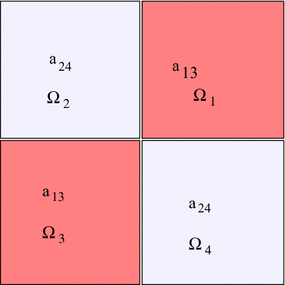

  

  Kellog’s test: $\varOmega _i,{ }i=1,\ldots ,4$

  Table 2 Kellog’s test: the convergence rates

  $$\begin{aligned} \varphi (\theta ) \!=\! {\left\{ \begin{array}{ll} \cos ( (\pi /2 \!-\!\sigma )\lambda ) \cos ((\theta -\pi /2\!+\!\rho )\lambda ), &{}\quad \text {if }\quad 0\le \theta \!<\! \pi / 2, \\ \cos (\rho \lambda ) \cos ((\theta -\pi +\sigma )\lambda ), &{}\quad \text {if }\quad \pi /2 \le \theta \!<\! \pi , \\ \cos (\sigma \lambda ) \cos ((\theta -\pi -\rho )\lambda ), &{}\quad \text {if }\quad \pi \le \theta \!<\! 3\pi /2 , \\ \cos ( (\pi /2 \!-\!\rho )\lambda ) \cos ((\theta \!-\!3\pi /2\!-\!\sigma )\lambda ),&{}\quad \text {if } 3 \pi /2 \le \theta \!\le \! 2\pi , \end{array}\right. } \end{aligned}$$

  and the numbers $\lambda , \rho , \sigma$ satisfy the nonlinear relations

  $$\begin{aligned} {\left\{ \begin{array}{ll} -\tan ((\pi /2 -\sigma )\lambda ) \cot (\rho \lambda )= \mathcal {R},\\ -\tan (\rho \lambda )\cot (\sigma \lambda ) = 1 / \mathcal {R},\\ -\tan (\sigma \lambda )\cot ((\pi /2-\rho )\lambda ) = \mathcal {R},\\ 0<\lambda<2,\\ \max \{0,\pi \lambda -\pi \}<2\lambda \rho<\min \{\pi \lambda ,\pi \},\\ \max \{0,\pi - \pi \lambda \}<-2\lambda \sigma <\min \{\pi ,2\pi -\lambda \pi \}, \end{array}\right. } \end{aligned}$$

  (6.1)

  where $\mathcal {R}:=\alpha _{13} / \alpha _{24}$. The above system of equations admits several solutions. For this example, we set $\lambda =0.3$, and $\rho =\pi /4$. A Newton iteration recovers one solution for the rest of the parameters, namely $\sigma = -4.4505895927$ and $\mathcal {R}=17.34972217$. Note that in this case $u\in W^{1.3,2}(\varOmega )$. We solved the problem using B-spline spaces with degree $k=2$. In Table 2, we display the convergence rates of the error. We can see that, the experimental convergence rates approach the value 0.3, which is in agreement with the regularity of the solution and (5.27).

• 3 Circular sector domain, non-matching meshes

  Consider the problem on a circular sector domain described in polar coordinates as $\varOmega =\{( r,\phi ): 0\le r\le 3, 0\le \phi \le \frac{\pi }{2}\}$. The diffusion coefficient is set to be uniformly $\alpha =1$ in $\varOmega$, the function f and the boundary condition $u_D$ in (2.1) are determined to have exact solution $u(x,y)=\sin (2\pi x)\sin (2 \pi y)$. The domain $\varOmega$ is divided into two subdomains $\varOmega _1$ (circular sector) and $\varOmega _2$ (annulus) and non-matching meshes are considered, as it is presented in Fig. 3. We performed three numerical tests, where the mesh size $h_1$ of the circular sector and the mesh size $h_2$ of the annulus are such that $\frac{h_1}{h_2}=\kappa$ with $\kappa =2,4$ and 8 correspondingly. The results for the three test cases are displayed in Table 3. The second, fourth and sixth column include the error ${\Vert u_h - u\Vert _{dG(\varOmega )} }$ values. The third, the fifth and the seventh column include the convergence rates of the error for the different ratio $\kappa$. We observe that the convergence rates for all cases of the non-matching meshes, tend to get the optimal value with respect to the B-spline degree $k=2$, (see also estimate (4.27c)). Thus, for this problem the different grid sizes of the subdomains do not influence the behavior of the convergence rate. We point out that for the present example the point (0, 0) is a singular point and the Jacobian determinant is vanished. As we have seen in the results in Table 3, this singularity of the mapping did not affect the convergence rates. However, if we continue the refinement steps reaching the limits of our code, we would have numerical problems. This occurs, because in that case, the quadrature points would be located too close to the singularity of the mapping, and thus we might be lead to division by (almost) zero while performing the numerical integration. We mention that, similar type problems, where the parametrization mappings have singular points, have been solved and discussed more thoroughly by the authors in [23].

Fig. 3

Circular sector: the two subdomains

Table 3 Circular sector: the $\Vert u-u_h\Vert _{dG(\varOmega )}$ values and the convergence rates for $h_1/h_2=\kappa$

7 Conclusions

In this paper, we presented theoretical error estimates of the dG-IgA method applied to a model elliptic problem with discontinuous coefficients. The problem was discretized according to IgA methodology using discontinuous $\mathbb {B}$-spline spaces. Due to global discontinuity of the approximate solution on the subdomain interfaces, dG discretizations techniques were utilized. In the first part, we assumed higher regularity for the exact solution, that is $u\in W^{l\ge 2,2}$, and we showed optimal error estimates with respect to $\Vert .\Vert _{dG}$. In the second part, we assumed low regularity for the exact solution, that is $u\in W^{l,p}$ for $l\ge 2$ and $p\in (\frac{2d}{d+2(l-1)},2)$, applying the Sobolev embedding theorem we proved optimal convergence rates with respect to $\Vert .\Vert _{dG}$. The theoretical error estimates were validated by numerical tests. The results can obviously be carried over to diffusion problems on open and closed surfaces as studied in [24], and to more general second-order boundary value problems like linear elasticity problems as studied in [2].

References

Adams, R.A., Fournier, J.J.F.: Sobolev Spaces, Pure and Applied Mathematics, 2nd edn. ACADEMIC PRESS-imprint Elsevier Science, Netherlands (2003)
Apostolatos, A., Schmidt, R., Wüchner, R., Bletzinger, K.U.: A Nitsche-type formulation and comparison of the most common domain decomposition methods in isogeometric analysis. Int. J. Numer. Methods Eng. 97(7), 1099–1142 (2014)
Arnold, D.N., Brezzi, F., Cockburn, B., Marini, D.L.: Unified analysis of discontinuous Galerkin methods for elliptic problem. SIAM J. Numer. Anal. 39(5), 1749–1779 (2002)
Bazilevs, Y., Hughes, T.J.R.: NURBS-based isogeometric analysis for the computation of flows about rotating components. Comput. Mech. 43, 143–150 (2008)
Bazilevs, Y., da Veiga, L.B., Cottrell, J.A., Hughes, T.J.R., Sangalli, G.: Isogeometric analysis: approximation, stability and error estimates for \(h\)-refined meshes. Math. Models Methods Appl. Sci. 16(7), 1031–1090 (2006)
Brener, S.C., Scott, L.R.: The mathematical Theory of Finite Element Methods, Texts in Applied Mathematics, 3rd edn. Springer, New York (2008)
Brunero, F.: Discontinuous Galerkin methods for isogeometric analysis. Master’s thesis, Università degli Studi di Milano (2012)
Ciarlet, P.G.: The Finite Element Method for Elliptic Problems. Studies in Mathematics and its Applications. North Holland Publishing Company, Amsterdam (1978)
Cotrell, J.A., Hughes, T.J.R., Bazilevs, Y.: Isogeometric Analysis. Toward Integration of CAD and FEA. Wiley, United Kingdom (2009)
Dryja, M.: On discontinuous Galerkin methods for elliptic problems with discontinuous coefficients. Comput. Methods Appl. Math. 3(1), 76–85 (2003)
Dryja, M., Galvis, J., Sarkis, M.: BDDC methods for discontinuous Galerkin discretization of elliptic problems. J. Complex. 23, 715–739 (2007)
Evans, J.A., Hughes, T.J.R.: Isogeometric Divergence-conforming B-splines for the Darcy-Stokes-Brinkman equations. Math. Models Methods Appl. Sci. 23(4), 671–741 (2013)
Evans, L.C.: Partial Differential Equations, Graduate Studies in Mathematics, 2nd edn. American Mathematical Society, Providence (2010)
Feng, X., Karakashian, O.A.: Two-level additive Schwarz methods for a discontinuous Galerkin approximation of second order elliptic problems. SIAM J. Numer. Anal 39(4), 1343–1365 (2001)
Grisvard, P.: Elliptic Problems in Nonsmooth Domains in Classics in Applied Mathematics. SIAM, Philadelphia (2011)
Heinrich, B., Nicaise, S.: The Nitsche mortar finite-element method for transmission problems with singularities. IMA J. Numer. Anal 23, 331–358 (2003)
Hughes, T.J.R.: The Finite Element Method: Linear Static and Dynamic Finite Element Analysis. Dover Publications, New York (2000)
Hughes, T.J.R., Cottrell, J.A., Bazilevs, Y.: Isogeometric analysis: CAD, finite elements, NURBS, exact geometry and mesh refinement. Comput. Methods Appl. Mech. Eng. 194, 4135–4195 (2005)
Kellogg, R.B.: On the Poisson equation with intersecting interfaces. Appl. Anal. 4, 101–129 (1975)
Kleiss, S.K., Pechstein, C., Jüttler, B., Tomar, S.: IETI - Isogeometric Tearing and Interconnecting. Comput. Methods Appl. Mech. Eng. 247–248, 201–215 (2012)
Knees, D.: On the regularity of weak solutions of quasi-linear elliptic transmission problems on polyhedral domains. Z. Anal. Anwendungen 23(3), 509–546 (2004)
Korneev, V.: Skhemy metoda konechnykh elementov vysokikh poryadkov tochnosti (Finite Element Schemes of high-order Accuracy). Izd-vo Leningradskogo gos. universiteta, Leningrad (1977). (in Russian)
Langer, U., Mantzaflaris, A., Moore, S.E., Toulopoulos, I.: Mesh grading in isogeometric analysis. Computers Math. Appl. 70(7), 1685–1700 (2015)
Langer, U., Moore, S.E.: Discontinuous Galerkin isogeometric analysis of elliptic PDEs on surfaces. NFN Technical Report 12, Johannes Kepler University Linz, NFN Geometry and Simulation, Linz (2014). Also available at http://arxiv.org/abs/1402.1185, and accepted for publication in the proceedings of the 22nd International Domain Decomposition Conference held at Lugano, Switzerland, September 2013
Li, B.Q.: Discontinuous Finite Element in Fluid Dynamics and Heat Transfer. Computational Fluid and Solid Mechanics. Springer, New York (2006)
Pietro, D.A.D., Ern, A.: Analysis of a discontinuous Galerkin method for heterogeneous diffusion problems with low-regularity solutions. Numer. Methods Partial Differ. Equ. 28(4), 1161–1177 (2012)
Pietro, D.A.D., Ern, A.: Mathematical Aspects of Discontinuous Galerkin Methods (Mathmatiques et Applications), Mathmatiques et Applications. Springer, Berlin (2012)
Pigl, L.A., Tiller, W.: The NURBS Book, Monographs in Visual Communication, 2nd edn. Springer, Berlin (1997)
Riviere, B.: Discontinuous Galerkin methods for Solving Elliptic and Parabolic Equations. SIAM, Society for Industrial and Applied Mathematics, Philadelphia (2008)
Schumaker, L.L.: Spline Functions: Basic Theory, 3rd edn. University Press, Cambridge, Cambridge (2007)
Toulopoulos, I.: An interior penalty discontinuous Galerkin finite element method for quasilinear parabolic problems. Finite Elements in Analysis and Design 95, 42–50 (2015)
Turek, S.: Efficient Solvers for Incompressible Flow Problems: An Algorithmic and Computational Approach. Lecture Notes in Computational Science and Engineering. Springer, Berlin (2013)
da Veiga, L.B., Buffa, A., Rivas, J., Sangalli, G.: Some estimates for \(hpk-\) refinement in Isogeometric Analysis. Numer. Math. 118(7), 271–305 (2011)
da Veiga, L.B., Cho, D., Pavarino, L., Scacchi, S.: BDDC preconditioners for isogeometric analysis. Math. Models Methods Appl. Sci. 23(6), 1099–1142 (2013)
Wihler, T.P., Riviere, B.: Discontinuous Galerkin methods for second-order elliptic PDE with low-regularity solutions. J. Sci. Comput. 46(2), 151–165 (2011)
Zlamál, M.: The finite element method in domains with curved boundaries. Int. J. Numer. Methods Eng. 5(3), 367–373 (1973)
Acknowledgments
The authors thank A. Mantzaflaris, S. Moore and C. Hofer for their help on performing the numerical tests. This work was supported by Austrian Science Fund (FWF) under the grant NFN S117-03.
Author information
Authors and Affiliations
Corresponding author
Additional information
Communicated by Gabriel Wittum.
Rights and permissions
About this article
Cite this article
Langer, U., Toulopoulos, I. Analysis of multipatch discontinuous Galerkin IgA approximations to elliptic boundary value problems. Comput. Visual Sci. 17, 217–233 (2015). https://doi.org/10.1007/s00791-016-0262-6
Received:
Accepted:
Published:
Issue Date:
DOI: https://doi.org/10.1007/s00791-016-0262-6
Keywords
- Linear elliptic problems
- Discontinuous coefficients
- Discontinuous Galerkin discretization
- Isogeometric analysis
- Non-matching meshes