
Abstract
In this paper, we investigate some aspects of Spencer–Brown’s Calculus of Indications. Drawing from earlier work by Kauffman and Varela, we present a new categorical framework that allows to characterize the construction of infinite arithmetic expressions as sequences taking values in grossone.
1 Introduction
The Calculus of Indications (Spencer-Brown 1969) provides an elegant formalism to represent fundamental logical operations as nested “distinctions” notated as closed curves in a plane.Footnote 1 An especially interesting phenomenon in the Calculus of Indications (CI) is what Spencer Brown calls the reentry of the form, understood as the recursive nesting of curves yielding a structure formally equivalent to the Epimenides paradox (or the Liar Paradox (Barwise and Etchemendy 1989)]. As in the classical setting, there are several different attempts made at resolving the paradoxical character of this self-referential or “reentered” form. One, proposed first by Spencer Brown himself and advanced more rigorously in Kauffman and Varela (1980), basically defines an alternative truth value, the “imaginary” value which is neither true nor false. The other, introduced in Varela and Goguen (1978), takes the limit of the nesting process to yield a definite expression that is then taken as a particular solution to a given reentry equation, rather than a distinct general truth value.
We will take an intermediate route between these two approaches, combining the best of the two methods in a category-theoretical setting. We will show first how in the case of expressions consisting of finite nestings, a recursive procedure yields a unique answer as the formal simplification or reduction of the given expression. However, in order to extend our procedure then to the case of infinite nestings, we will have to develop the notion of constructive sequences that build up such expressions part by part. In evaluating such sequences, we will need to deal with infinite sums that, in general, diverge. A finer control on such divergence is needed in order to make the process of evaluating sequences well-defined, and a solution to this problem is offered by the notion of grossone, first defined by Yaroslav Sergeyev, with respect to which the natural numbers (including zero) can be represented by the sequence  .Footnote 2
In the approach detailed below, incorporating calculations with ① allows for the evaluation function applied to both finite and infinite graphs to yield a distinguished, computable answer, solving the question of how to give a truth value to the reentry of the form with respect to constructive sequences. We therefore aim to capitalize on the basic idea that grossone allows for a “finer” control on infinite denumerable sequences than the classic Cantorian approach (for details, see Sergeyev’s survey paper 2017 and, for a more informal treatment, Sergeyev (2013a)). Within the grossone framework, it becomes feasible to deal computationally with infinite quantities, in a way that is both new (in the sense that previously intractable problems become amenable to computation) and natural.Footnote 3
The CI is generated by two simple algebraic rules or “initials” applicable to diagrams called “arithmetic expressions” consisting of collections of non-intersecting closed curves in the Euclidean plane (Fig. 1).
The lack of expression on the right side of initial 2 is merely apparent. For CI, the empty plane (or any empty part of the plane) is also a formal expression (or part of an expression) in the calculus. It is this use of natural topological properties of closed curves in the plane that makes CI particularly interesting as a diagrammatic formal system, as recognized for instance by Louis Kauffman in Kauffman (2012).
Using the two initials as permissions for rewriting equivalent expressions, it becomes possible to simplify such expressions step by step. For instance, the sequence of expressions below represents an application of initial 2, an application of initial 1 and then another application of initial 2 (Fig. 2).
In developing the system of CI, Spencer Brown first considers arithmetic expressions composed of finite collections of closed curves. He calls the system consisting of all such expressions as related algebraically via the two initials schematized above the Primary Arithmetic. He then introduces variables that may take such expressions as values and calls the system of expanded expressions the Primary Algebra, demonstrating standard results of consistency
and completeness for the resulting system which is equivalent to that of Classical Propositional Logic. We will be especially concerned in the present paper with the introduction of infinite expressions (infinite collections of non-intersecting closed curves in the Euclidean plane) into the system, which are described in Spencer-Brown (1969) in terms of equations of second degree and the distinctive notion of “reentry of the form”.
In developing the system of CI, Spencer Brown first considers arithmetic expressions composed of finite collections of closed curves. He calls the system consisting of all such expressions as related algebraically via the two initials schematized above the Primary Arithmetic. He then introduces variables that may take such expressions as values and calls the system of expanded expressions the Primary Algebra, demonstrating standard results of consistency and completeness for the resulting system which is equivalent to that of Classical Propositional Logic. We will be especially concerned in the present paper with the introduction of infinite expressions (infinite collections of non-intersecting closed curves in the Euclidean plane) into the system, which are described in Spencer-Brown (1969) in terms of equations of second degree and the distinctive notion of “reentry of the form”.

Algebraic rules

Reduction process
It may be remarked that the system of CI’s Primary Algebra is quite close in spirit to the earlier logical system of Existential Graphs (EG) developed by C.S. Peirce. In particular, the expressions of Spencer Brown’s CI Primary Algebra are formally equivalent to those of Peirce’s EG-\(\alpha \), which was also designed to express Classical Propositional Logic. However, whereas Peirce elects to consider the empty plane (which he calls the “Sheet of Assertion”) to express the value TRUE, Spencer Brown takes the empty sheet to express the value FALSE. In a corresponding manner, a single empty curve or “cut” represents the value FALSE for Peirce and the value TRUE for Spencer Brown. In accordance with this difference, for Peirce the juxtaposition of two or more notational elements (either “cuts” or variables) expresses their conjunction, while for Spencer Brown such a juxtaposition represents their disjunction. For both systems, a curve or “cut” negates the value of its interior. The expressions of the two systems are thus syntactically equivalent but interpreted inversely at the semantic level.Footnote 4
In what follows, we will not further examine the standard algebraic treatment of the Calculus of Indications in which variables in expressions of the Primary Algebra may take basic arithmetic expressions as values (by substituting such expressions diagrammatically for the variables themselves, thus reducing expressions in the Primary Algebra to expressions in the Primary Arithmetic). Instead, we will develop an alternate algebra of constructive sequences of arithmetic expressions themselves. This algebra of constructive sequences concerns the extension, proposed by Spencer Brown himself but not fully developed in Spencer-Brown (1969), of expressions in the Primary Arithmetic to include infinite collections of closed curves in the plane. Following the lead of Peirce, we will refer to the closed curves in all such expressions in what follows as “cuts”.
One of the most interesting features of CI is the idea initially proposed in Spencer-Brown (1969) that solutions for equations such as the following may be expressed as infinite recursive structures.
Consider, for instance, the following “equation” (Fig. 3).
Clearly, neither the substitution of the empty sheet nor the substitution of the empty cut for A (nor any finite expression, since all such expressions reduce to either the empty sheet or the empty cut) will satisfy the above equation. The following expression, however, does formally satisfy it, where the filled innermost circle is meant to represent an infinite sequence of further nested circles (Fig. 4).

Recursive structure

Infinite nesting
In order to simplify the notation, in what follows we will denote the above expression (an infinite series of single nested cuts) with the symbol I.
The expression above may itself be constructed by a recursive procedure that in effect operationalizes the original equation 1. Informally, I is generated by treating the right side of equation 1 as an operation that draws a circle around A. Starting from \(A =\) empty sheet, one then successively plugs in the result of the operation back into the equation and repeats the operation indefinitely. The original equation thus becomes a recipe for generating an expression that is a solution to the equation itself.Footnote 5
This is why Spencer Brown named such recursive constructions “reentry of the form”. His own interpretation of this notation was in terms of temporal signals. The solution to the equation above would be conceived as an infinite nesting of circles, and on this interpretation its value would be understood as an oscillation between TRUE and FALSE.
The notion of “reentry of the form” has been analyzed and evaluated by various specialists including mathematicians, logicians, and social scientists. Especially noteworthy is the use of CI and reentry as the basis for a comprehensive theory of social communicative systems in Luhmann (1995) and its related research program.
From a more formal point of view, two dominant approaches to reentry in CI may be identified. The first, represented by Kauffman and Varela (1980) and Zalamea (2010) works from the intuition first proposed by Spencer Brown that the infinitely-nested expression that stands as a solution to equation 1 may be understood on analogy with the imaginary value i in complex algebra. Spencer Brown thus calls the value of the CI-expression I the “imaginary value”. Somewhat surprisingly, this informal analogy may be made rigorous, as shown in Kauffman and Varela (1980). More recently, Zalamea (2010) has developed this approach (though with primary reference to Peirce’s EG rather than Spencer Brown’s CI) with respect to holomorphic functions. The second approach is represented by Varela and Goguen (1978). According to this approach, infinite expressions are conceived on analogy with limits of infinite sequences. If the former approach follows the mathematics of complex algebra, this latter approach follows instead that of differential calculus. Our own approach detailed in what follows represents something of a hybrid model between the two previous approaches.Footnote 6
2 The category \({\mathcal {CI}}\) of CI-expressions
In this section, we develop a formalization of the Calculus of Indications in the setting of category theory, in particular, by using categories of presheaves. This approach follows that introduced in Caterina and Gangle (2016) and Caterina and Gangle (2013). The elementary notions of category theory are summarized here for the reader’s convenience. For further details, the reader is directed to Mac Lane (1998).
A category consists of a class of objects together with morphisms or arrows between objects. Given two objects a and b a morphism f between them will be denoted either \(f: a \rightarrow b\) or \(a {\mathop {\rightarrow }\limits ^{f}} b\). A category is subject to axioms of identity (every object a is equipped with an identity morphism, \(a {\mathop {\rightarrow }\limits ^{1_a}} a\)), composition (two morphisms, \(a {\mathop {\rightarrow }\limits ^{f}} b\) and \(b {\mathop {\rightarrow }\limits ^{g}} c\) compose to a unique morphism \(a {\mathop {\rightarrow }\limits ^{g\circ f}} c\), where \(\circ \) indicates the operation of composition) and associativity (paths of morphisms compose uniquely, i.e., given three arrows \(f: a \rightarrow b, g: b \rightarrow c\) and \(h: c \rightarrow d\), \(h \circ (g \circ f) = (h \circ g) \circ f\), given the same morphism from a to d).
A functor F is a map between two categories (say \(\mathcal {A}\) and \(\mathcal {B}\)), sending objects to objects and morphisms to morphisms in a way that preserves identities and composition. If for any morphism \(a \rightarrow a^{\prime }\) in \(\mathcal {A}\), \(F(a \rightarrow a^{\prime })\) is mapped to a morphism \(F(a) \rightarrow F(a^{\prime })\) in \(\mathcal {B}\), F is said to be covariant. If instead \(F(a \rightarrow a^{\prime })\) maps to \(F(a) \leftarrow F(a^{\prime })\), F is called contravariant.
With these core notions in hand, we may now define the notion of an expression in CI as a contravariant functor from the category of natural numbers to that of finite sets. More precisely:
Definition 1
A CI-expression is a functor
where \({\mathbb {N}}^{op}\) is the category of natural numbers with the usual order reversedFootnote 7 and FinSet is the category whose objects are finite sets and whose morphisms are functions between them. We call a CI-expression finiteFootnote 8 if and only if there exists some \(n\in {\mathbb {N}}\) such that \(F(n)=\emptyset \), otherwise we call it infinite.
The collection of all CI-expressions so defined forms a category, with natural transformations between CI-expressions as morphisms. Such a category is typically denoted by \({\mathbf{FinSet}^{\mathbb {N}}}^{op}\). For the sake of notational simplicity, we label this category \({\mathcal {CI}}\). Thus, \({\mathcal {CI}}={\mathbf{FinSet}^{\mathbb {N}}}^{op}\).
It is a standard result that, since \({\mathcal {CI}}\) is a category of presheaves (with the domain category being small), it has the structure of a topos. This means, in particular, that it can be endowed with a logical structure. In particular, it possesses a subobject classifier that functions in the topos in a manner analogous to the set \(\left\{ 0,1\right\} \) in the category Set (also a topos) of sets and functions. Just as morphisms (functions) from any set S into \(\left\{ 0,1\right\} \) correspond to subsets of S, morphisms from any object O in a general topos into the subobject classifier of the topos correspond to monic arrows into O.Footnote 9
Using the notion of monic arrows, it is straightforward to define a preorder \(\preceq \) on the objects of \({\mathcal {CI}}\). Given two such objects \(O_1\) and \(O_2\), \(O_1\preceq O_2\) iff there is a monic arrow \(m:O_1\longrightarrow O_2\).
In the case of the category \({\mathcal {CI}}\), monic arrows select “parts” of CI-expressions in the sense that they select arbitrary cuts in the target expression subject to the condition that if they select a cut c, they also select all cuts C such that c is inside C. This is illustrated by the following example (Fig. 5).
Given the following two CI-expressions
monic morphisms from the former to the latter correspond to selections of parts of the latter. There are exactly three such morphisms, represented here by thickened lines (Fig. 6).
The mathematical setting of category theory, and in particular presheaves, allows for a rigorous formalization of the somewhat informal approach found in Varela and Goguen (1978).
In any topos of presheaves, each object in the base category gives rise to a canonical presheaf associated with that object called a representable set. For details, see Reyes et al. (2004) and Gangle et al. (2020). In the topos \({\mathcal {CI}}\), we have a representable set \(h_n\) for every \(n\in {\mathbb {N}}\), which consists of n nested circles.
Morphisms from representable sets \(h_n\) into a CI-expression F correspond uniquely to cuts in F at depth n. We may thereby identify cuts \(p, q, r\dots \) in any CI-expression with morphisms \(p: h_{n^p}\longrightarrow F, q: h_{n^q}\longrightarrow F, r:h_{n^r}\longrightarrow F\dots \), where \(h_{n^x}\) represents a representable set with as many nested cuts as the depth of x.

CI-expressions

List of morphisms
Thus with representable sets, we have a straightforward way to characterize formally when one cut is inside another and also when a cut is empty. Given a CI-expression F, a cut q at depth n in F is inside a cut p at depth m in F if and only if the following diagram is well-defined and commutes (Fig. 7).
A cut is empty if no cuts are inside it. Using this framework, it becomes possible to formally define various diagrammatic operations on CI-expressions. We define a pair of such operations, a unary operation CIRCLE and a binary operation JUXTAPOSE:
Definition 2
-
CIRCLE: given a CI-expression F it generates a new CI-expression C(F) such that \(C(F)(1)=\{ \emptyset \}\) and for all \(n\in {\mathbb {N}}\), \(C(F)(n+1)=F(n)\) and \(C(F)({i_{n+1}}):C(F)(n+2)\longrightarrow C(F)(n+1) = F({i_n}): F(n+1) \longrightarrow F(n)\), where morphisms \(i_n\) are the (unique) morphisms from n to \(n+1\).
-
JUXTAPOSE: given two CI-expressions F and G it generates a new CI-expression J(F, G), consisting of the categorical coproduct \(F\coprod G\) of F and G.Footnote 10
Remark 1
In any category C the coproduct of two objects A and \(A^{\prime }\), denoted by \(A \coprod A^{\prime }\) is an object endowed with two arrows \(p_1: A \coprod A^{\prime } \leftarrow A\) and \(p_2: A \coprod A^{\prime } \leftarrow A^{\prime } \) such that, for all objects T with two arrows f and g respectively from A and \(A'\) into T, there exists a unique morphism \(!h: T \leftarrow A \coprod A^{\prime }\) that makes the diagram in Fig. 8 commute.

Cut inclusion

Coproduct
Diagrammatically, CIRCLE generates a new CI-expression by drawing a circle (more generally, a closed curve) around a given CI-expression. Similarly, the operation JUXTAPOSE applied to two CI-expressions generates the CI-expression consisting of both expressions drawn next to one another on the same plane.
3 Evaluating the objects of \({\mathcal {CI}}\)
Each finite object in \({\mathcal {CI}}\) takes a unique value according the following algorithmic evaluation procedure.
Definition 3
Given a finite CI-expression \(F \in \text{ Obj }({\mathcal {CI}})\), a recursive evaluation of F, denoted by RE(F) is an element of \(\left\{ 0,1\right\} \) generated by a finite sequence \(f_1, f_2,\dots , f_n\) of subobjects of F such that \(f_1=F\) and each step from \(f_i\) to \(f_{i+1}\) corresponds to an application of the “pruning procedure” algorithm detailed below. Since that algorithm ensures that each of its operations generates a proper subobject of its operand, the sequence \(f_1, f_2,\dots , f_n\) is ordered \(f_1 \succ f_2 \succ \dots \succ f_n\) Additionally, since the elements in RE(F) are ordered by inclusion, they may be thought of as a path in the lattice Sub(F).
We define a successor of a cut n in a CI-expression F as a cut that appears immediately inside n in F. Note that successors are not necessarily unique. An empty cut is a cut that has no successors. An eliminable cut is a cut with at least one successor that is empty.
Given a finite CI-expression F, we reduce it to one of the two values 0 or 1 by applying the following iterative pruning procedure:
Procedure 1
-
(i)
Consider the diagrammatic representation of F as a collection of nested cuts.
-
(ii)
Take any eliminable cut n in F.
-
(iii)
Erase the cut n and all cuts inside it, yielding a new CI-expression \(F^\prime \).
-
(iv)
Replace F with \(F^\prime \) and repeat (ii) and (iii) until the CI-expression \(F^\prime \) is either blank (no cuts at all) or consists of empty cuts only.
-
(v)
If the final CI-expression \(F^\prime \) is blank, assign the original CI-expression F the value 1. Otherwise, assign F the value 0.Footnote 11
Every time steps (ii) and (iii) of the procedure are applied, a choice must be made among all the eliminable cuts that exist at that stage. But any variant sequence of such choices leads nonetheless invariably to the same final result:
Theorem 1
Given a finite expression F, the algorithm outlined in Procedure 1 will output either the empty sheet or a finite number of empty cuts, independently of the choices made in step (ii), that is, the order in which the eliminable cuts are chosen.
Proof
We first label all the nodes of F either 0 or 1 according to the following rule:
-
All cuts are labeled 0 if they have at least one successor labeled 1 and they are labeled 1 otherwise.
It should be clear that this labeling is well-defined and uniquely determined for any finite expression. We note first that prior to applying the pruning procedure every empty cut of the expression is necessarily labeled 1 since these (by definition) have no successors. We then note that repeated applications of steps (ii) and (iii) in the pruning procedure above will always select and delete a cut labeled 0. It is impossible for a node labeled 1 to have any successors also labeled 1 according to the labeling rule. Since only an eliminable cut can be chosen and deleted in steps (ii) and (iii), no such cut can ever be labeled 1. Thus every cut selected in step (ii) must be labeled 0.
Eventually, all cuts labeled 0 must be deleted. This will result in a final expression that has at most depth 1. \(\square \)
4 Evaluating infinite objects in \({\mathcal {CI}}\)
In this section, we turn our attention to infinite objects in the Calculus of Indications, and following the lead of Varela and Goguen (1978) we consider them from the point of view of limits of sequences of finite expressions that “construct” or “build” them step by step. In the first subsection, the informal presentation in Varela and Goguen (1978) is given a rigorous mathematical setting in the framework of presheaves developed above. We then show how every constructive sequence gives rise to a unique value in the grossone framework. Finally, we define an algebra on the sequences that behaves nicely with respect to valuations in the interval [0, ① ].
4.1 Constructive sequences of CI-expressions
Definition 4
A constructive sequence for a CI-expression F is an infinite sequence of finite CI-expressions, \(f_1, f_2, f_3, \dots \) such that for all i \(f_{i} \preceq f_{i+1} \preceq F\) and for any m and any morphism \(x:h_m \rightarrow F\) there is \(n\in {\mathbb {N}}\) such that the following diagram commutes. (The representable set \(h_m\) factors through \(f_n\) into F) (Fig. 9).

Constructive sequences
We designate constructive sequences for CI-expressions \(F, G, \dots \) with Greek letters and capital Roman subscripts \(\alpha _F, \beta _F, \dots , \alpha _G, \beta _G, \dots \), dropping the subscripts if the given CI-expression is either obvious from the context or else left indeterminate.
Intuitively, a constructive sequence may be thought of as an increasingly determined CI-expression that in the limit converges on F. This is the guiding intuition behind the approach to CI found in Varela and Goguen (1978) which the present paper develops somewhat more rigorously. Each step in the sequence may be thought of as the inscribing of CI-expressions on areas of the CI-expression formed at the previous step. Constructive sequences are thus formal characterizations of the informal notion of “growing” or “deepening” CI-expressions.
Definition 5
An s-evaluation \(sval(\alpha )\) for a constructive sequence \(\alpha \) is an infinite binary sequence, that is, a function \({\mathbb {N}}\longrightarrow \left\{ 0,1\right\} \), such that \(sval(\alpha )(n) = RE(\alpha _n)\).
Such a sequence is obviously constructible, given any constructive sequence \(\alpha \), since the calculation of \(RE(\alpha _n)\) for every n is itself a finite procedure.
Definition 6
Given \(k\in {\mathbb {N}}\) a k-sum \(S_k(\alpha )\) for a constructive sequence \(\alpha \) is
It may be remarked that given any constructive sequence \(\alpha _F\) for any finite CI-expression F such that \(RE(F) = 1\), the limit of the k-sum as k approaches infinity will be infinite. That is,
Conversely, given any constructive sequence \(\beta _G\) for any finite CI-expression G such that \(RE(G) = 0\), the limit of the k-sum as k approaches infinity will be finite or zero. That is,
for some \(n\in {{\mathbb {N}}}\).
In order to normalize k-sums for different values of k, it is natural to define a k-value in the following way:
Definition 7
A k-value \(V_k(\alpha )\) for a constructive sequence \(\alpha \) and some \(k\in {\mathbb {N}}\) is \(\frac{S_k(\alpha )}{k}\).
We now define the following pair of operations on constructive sequences, a unary operation CIRC and a binary operation JUXTA:
-
1.
CIRC: Given a sequence \(\alpha \), the sequence CIRC(\(\alpha \)) or
 is the sequence that draws a cut around each expression in the sequence. Formally,
  \(=\) CIRCLE(\(f_1\)), \(\ldots \), CIRCLE(\(f_n\)), \(\ldots \)Footnote 12
 -
2.
JUXTA: Given two sequences \(\alpha = f_1, f_2, \ldots \) and \(\beta = g_1, g_2, \ldots \), the sequence JUXTA(\(\alpha , \beta \)) or \(\alpha \beta \) is the sequence that juxtaposes \(\alpha _n\) and \(\beta _n\) for all \(n\in {\mathbb {N}}\). Formally, \(\alpha \beta =\) \(J(f_1, g_1)\), \(J(f_2, g_2)\), \(\ldots \). It should be obvious that JUXTA, like the JUXTAPOSE operation J above, is a commutative operation.
 is the sequence that draws a cut around each expression in the sequence. Formally,
We have the following facts for all \(k\in {\mathbb {N}}\):
-
1.
\(S_k\)
 \( = k-S_k(\alpha )\)
 -
2.
\(S_k(\alpha \beta ) = {\sum _{n=1}^{k}} min(sval(\alpha ), sval(\beta )) \le S_k(\alpha )+S_k(\beta )\)

Our first result is to show that it is possible to extend these results to the entire sequence taken as a whole by using grossone.
A ① -sum  for a sequence \(\alpha \) is

Similarly, using the arithmetic properties of grossone, a ① -value  for a constructive sequence \(\alpha \) is
  .
.
In accord with the facts above, the following facts hold:
-
1.

-
2.


In addition, we have that:
-
3.
For any finite expression F and constructive sequence \(\alpha _F\),
 is either finite or ① -n for some finite n.
 is either finite or ① -n for some finite n.
From (3) and elementary divisibility properties of grossone, it follows that any constructive sequence G such that  with finite m and n must be the constructive sequence for an infinite expression.

All steps

Only even steps

Only odd steps
The use of the grossone notation and its associated arithmetic thus allows both for the uniform extension of certain finite determinations of constructive sequences to those sequences taken as a whole (that is, taken as “actual” or “completed” infinities) and also for a new arithmetic characterization (based solely on k-values) of the difference between finite and infinite CI-expressions.
4.2 Evaluating constructive sequences via grossone
We now show how every constructive sequence F gives rise to a unique value \(F_v\) such that  . Several examples will illustrate how the evaluation works.
Let us first look at the most basic reentry of the form considered in Fig. 3

which gives rise to the infinite nesting expression I as in Fig. 4 (as in Sect. 1, the solid dot stands for an infinite number of concentric circles):

The following three examples show three distinct constructive sequences, all of which construct I but each in a different way:
Example 1
This sequence includes every step of the recursive nesting, in which case each step is evaluated according to the sequence \(0,1,0,1,0,\dots \). Hence, the ① -sum is ① /2 and the ① -value is 1/2, which corresponds to Kauffman’s i (Fig. 10).

Varela’s equation

First three steps of the constructive sequence
Example 2
This sequence is constituted by the even steps of the recursive nesting only, each of which evaluates to 1, so that the ① -value of the entire sequence is ① (Fig. 11).
Example 3
Similarly, we can consider the sequence that only includes the odd steps of the recursive nesting, each of which evaluates to 0, hence the ① -value of the sequence is 0 (Fig. 12).
Example 4
Let us now consider a different and slightly more complex reentry of the form, via Varela’s equation (Fig. 13)
The first few steps of the recursive construction sequence are given below
Hence, since each step evaluates to 1, the ① -value of the constructive sequence that includes each recursive step is ① (Fig. 14).
5 Conclusion
It has been shown how both finite and infinite expressions in Spencer Brown’s Calculus of Indications may be straightforwardly represented in a category-theoretical setting as presheaves. We have denoted the resulting category of such presheaves (and natural transformations among them) as \({\mathcal {CI}}\). It was then shown how evaluations of finite expressions correspond to applications of a recursive procedure. In this setting, the concept of an infinite constructive sequence determining an expression as its limit was defined and used to define s-evaluations and k-sums and the latter’s normalized k-values for constructive sequences of finite expressions. The extension of these concepts to the case of infinite expressions was then shown to be possible by using the grossone notation and arithmetic framework.
A further, natural generalization is given by adding labels—representing atomic statements—to the Spencer–Brown, cuts-only graphs. In a recent paper Tohmé et al. (2020), we show that the grossone framework, combined with a different sets of tools from category theory, can be successfully employed also to deal with this more general case.
Notes
The introduction of the numeral ① may require, in some contexts, the augmentation of the set of natural \({\mathbb {N}}\) to a larger set \(\hat{{\mathbb {N}}}\), where
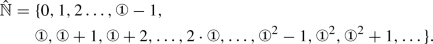
For the purpose of this paper we will not need to make use of \(\hat{{\mathbb {N}}}\).
Evidence of the efficacy of the grossone approach is highlighted by its successful application to many fields of applied mathematics, including optimization (see Cococcioni et al. 2018, 2020; De Cosmis and De Leone 2012; Sergeyev et al. 2018; Iavernaro et al. 2020; Iudin et al. 2012; Sergeyev 2007, 2013b; Zhigljavsky 2012), fractals and cellular automata (see Caldarola 2018; D’Alotto 2012, 2015, 2013) as well as infinite decision-making processes, game theory, and probability (see Fiaschi and Cococcioni 2018; Rizza 2018, 2019), whereas the formal logical foundation of grossone has been investigated in Lolli (2012); Margenstern (2011); Montagna et al. (2015). The approach presented in this paper bears similarities to the application of grossone to Turing machines as described in Sergeyev and Garro (2010). Further investigation of these analogies remains open.
The two systems are slightly different in terms of their rules of deduction (or rewriting). We do not examine this point any further in this paper.
The relevance of grossone to this construction will appear in the subsequent sections.
Here the objects are the natural numbers, and there is a morphism between two natural numbers \(m\rightarrow n\) if and only if \(m\ge n\). The choice of reversing the natural order is made in order for the functor F to be contravariant.
The condition given here guarantees that all nested cuts are of at most depth \(n-1\).
A monic arrow in any category is defined as follows. Given any morphism \(f: A\longrightarrow B\), f is said to be monic if, for any two morphisms \(g,h: Z\longrightarrow A\) such that \(f\circ g=f\circ h\), it is the case that \(g=h\).
\(\coprod \) is well defined in \({\mathcal {CI}}\) since it is a topos.
A formal categorical characterization of a variant of this procedure, applied to cuts-only \(\alpha \) graphs can found in Gangle et al. (2020).
Note that it is important to distinguish this operator
 (as an operation on \(\alpha \)) from the circle drawn around 1 in the grossone numeral ① .

 (as an operation on
 References
Barwise J, Etchemendy J (1989) The liar: an essay on truth and circularity. Oxford University Press, New York
Caldarola F (2018) The Sierpinski curve viewed by numerical computations with infinities and infinitesimals. Appl Math Comput 318:321–328
Caterina G, Gangle R (2013) Iconicity and abduction: a categorical approach to creative hypothesis-formation in Peirce’s existential graphs. Logic J IGPL 21(6):1028–1043
Caterina G, Gangle R (2016) Iconicity and abduction. Springer, New York
Cococcioni M, Pappalardo M, Sergeyev YD (2018) Lexicographic multi-objective linear programming using grossone methodology: theory and algorithm. Appl Math Comput 318:298–311
Cococcioni M, Cudazzo A, Pappalardo M, Sergeyev YD (2020) Solving the lexicographic multi-objective mixed-integer linear programming problem using branch-and-bound and grossone methodology. Commun Nonlinear Sci Numer Simul 84:1–20
D’Alotto L (2012) Cellular automata using infinite computations. Appl Math Comput 218(16):8077–8082
D’Alotto L (2013) A classification of two-dimensional cellular automata using infinite computations. Indian J Math 55:143–158
D’Alotto L (2015) A Classification of One-Dimensional Cellular Automata using Infinite Computations. Applied Mathematics and Computation 255:15–24
De Cosmis S, De Leone R (2012) The use of grossone in mathematical programming and operations research. Appl Math Comput 218(16):8029–8038
Fiaschi L, Cococcioni M (2018) Numerical asymptotic results in game theory using Sergeyev’s infinity computing. Int J Unconvent Comput 14(1):1–25
Gangle R, Caterina G, Tohme F (2020) A generic figures reconstruction of Peirce’s Existential Graphs (Alpha). Erkenntnis. https://doi.org/10.1007/s10670-019-00211-5
Iavernaro F, Mazzia F, Mukhametzhanov MS, Sergeyev YD (2020) Conjugate-symplecticity properties of Euler–Maclaurin methods and their implementation on the infinity computer. Appl Numer Math 155:58–72
Iudin D, Sergeyev YD, Hayakawa M (2012) Interpretation of percolation in terms of infinity computations. Appl Math Comput 218(16):8099–8111
Kauffman LH (2012) Laws of Form: an Exploration in Mathematics and Foundations. http://homepages.math.uic.edu/~kauffman/Laws.pdf
Kauffman LH, Varela FJ (1980) Form dynamics. J Soc Biol Struct 3:171–206
Lolli G (2012) Infinitesimals and infinites in the history of mathematics: a brief survey. Appl Math Comput 218(16):7979–7988
Luhmann N (1995) Social systems. Stanford University Press, Stanford
Mac Lane S (1998) Categories for the working mathematician. Springer, Berlin
Margenstern M (2011) Using Grossone to count the number of elements of infinite sets and the connection with bijections. p-Adic Numbers. Ultrametric Anal Appl 3(3):196–204
Montagna F, Simi G, Sorbi A (2015) Taking the Pirahã seriously. Commun Nonlinear Sci Numer Simul 21(1–3):52–69
Reyes M, Reyes G, Zolfaghari H (2004) Generic figures and their glueings. Polimetrica, Milan
Rizza D (2018) A study of mathematical determination through Bertrand’s Paradox. Philosophia Mathematica 26(3):375–395
Rizza D (2019) Numerical methods for infinite decision-making processes. Int J Unconvent Comput 14(2):139–158
Sergeyev YD (2013a). Arithmetic of infinity. Edizioni Orizzonti Meridionali, 2nd edition
Sergeyev YD (2007) Blinking fractals and their quantitative analysis using infinite and infinitesimal numbers. Chaos, Solitons Fract 33:50–75
Sergeyev YD (2010) Computer system for storing infinite, infinitesimal, and finite quantities and executing arithmetical operations with them. USA Patent 7(860):914
Sergeyev YD (2013b) Solving ordinary differential equations by working with infinitesimals numerically on the Infinity Computer. Appl Math Comput 219(22):10668–10681
Sergeyev YD (2017) Numerical infinities and infinitesimals: methodology, applications, and repercussions on two Hilbert problems. EMS Surv Math Sci 4(2):219–320
Sergeyev YD, Garro A (2010) Observability of turing machines: a refinement of the theory of computation. Informatica 21(3):425–454
Sergeyev YD, Kvasov DE, Mukhametzhanov MS (2018) On strong homogeneity of a class of global optimization algorithms working with infinite and infinitesimal scales. Commun Nonlinear Sci Numer Simul 59:319–330
Spencer-Brown G (1969) Laws of form. Allen & Unwin, London
Tohmé F, Caterina G, Gangle Rocco (2020) Computing Truth Values in the Topos of \(\alpha \)-Infinite Peirce’s Existential Graphs. In press, Applied Mathematics and Computation
Varela F, Goguen JA (1978) The arithmetic of closure. J Cybern 8:291–324
Zalamea F (2010) Towards a complex variable interpretation of Peirce’s existential graphs. In: Bergman M et al (eds) Ideas in action. Proceedings of the applying peirce conference, Nordic Pragmatism Network, Helsinki, pp 254–264
Zeman J (1974) Peirce’s logical graphs. Semiotica 12:239–256
Zhigljavsky A (2012) Computing sums of conditionally convergent and divergent series using the concept of Grossone. Appl Math Comput 218:8064–8076
Author information
Authors and Affiliations
Corresponding author
Ethics declarations
Conflict of interest
All authors declare that they have no conflict of interest.
Human and animal rights
This article does not contain any studies with human participants or animals performed by any of the authors.
Additional information
Communicated by Yaroslav D. Sergeyev.
Publisher's Note
Springer Nature remains neutral with regard to jurisdictional claims in published maps and institutional affiliations.
Rights and permissions
About this article

Cite this article
Gangle, R., Caterina, G. & Tohmé, F. A constructive sequence algebra for the calculus of indications. Soft Comput 24, 17621–17629 (2020). https://doi.org/10.1007/s00500-020-05121-1
Published:
Issue Date:
DOI: https://doi.org/10.1007/s00500-020-05121-1