
Abstract
Aiming to accurately assess the intensity of rockburst in coal mines, we propose a rockburst risk assessment model using the improved catastrophe progression method based on its sudden, complex, and non-linear characteristics. A risk assessment indicator system for rockburst is established based on the occurrence conditions of rockburst, which comprehensively considers 10 main influencing factors. We introduce a combined weighting method consisting of the variation coefficient method and analytic hierarchy process (AHP) to determine the weight and ranking of evaluation indicators, which improves the catastrophe progression method. Finally, by applying 10 coal mine cases into the established model and comparing them with the unimproved catastrophe progression method and several other risk assessment methods, we conclude that the accuracy of the model in assessing rockburst intensity level has increased by a maximum of 42.85%. Our work proves the effectiveness and practicality of the risk assessment model, which can provide good theoretical guidance for assessing rockburst intensity level in coal mines. Furthermore, based on the model risk assessment results and comparative analysis, this paper provides feasible suggestions for reducing the intensity of rockbursts.
1 Introduction
Rockburst is a coal-rock dynamic disaster characterized by its suddenness, complexity, and nonlinearity, resulting from the coupled effect of natural geological conditions and engineering disturbances (Wei et al. 2018; Wang and Du 2020; Mi et al. 2022; Yin et al. 2021). In recent years, with the increasing depth of coal mining, the in-situ stress increases constantly, and the geological and physical properties of coal seams and their roof and floor become more complex. Moreover, the influence of external dynamic load disturbances, such as large-scale roof movement and fault slip in the mining area, exacerbates the occurrence and severity of dynamic rockburst (Ranjith et al. 2017; Zhang et al. 2021a, b; Li et al. 2019; Gao et al. 2020; Zhang et al. 2023). As the most common type of coal mine disaster, dynamic rockburst not only causes significant economic losses but also poses a serious threat to the safety of workers (He et al. 2022; Cai et al. 2020). Therefore, it is of great significance to assess rockburst in a reasonable and accurate manner. However, due to its complexity, a sound risk assessment method system has not been established so far (Hou et al. 2021; Ghasemi et al. 2020).
Many scholars around the world have conducted extensive research on this and proposed numerous methods for assessing rockburst. According to different calculation methods, they are mainly divided into three categories: theoretical empirical analysis method, field monitoring and testing method, and applied mathematical model method (Li 2020) .
The theoretical empirical analysis method is a risk assessment method based on the mechanism of rockburst and engineering practice experience. Generally, it analyzes the stress–strain state of rock and combines it with existing evaluation indicators. Its biggest advantages are its low cost, simple operation, and strong practicality. However, this method involves past experience, which results in lower risk assessment accuracy. This type of method mainly includes strength theory empirical criterion (Ma et al. 2018), energy theory empirical criterion (Miao et al. 2016), brittleness theory criterion (Wang et al. 2015), and stiffness theory criterion (Tang and Xia 2010).
The field monitoring and testing method uses instruments to monitor certain necessary conditions for the occurrence of rockburst, or directly test the rock mechanical properties in the field to determine the possibility, timing, and range of its occurrence. The commonly used monitoring and testing methods include pulverized coal drilling cuttings method (He et al. 2021b, a), borehole stress meter method (Stas et al. 2007), support load method, roadway deformation measurement method, acoustic emission method (Zhai et al. 2020), microseismic method (Xue et al. 2021; Chen et al. 2022). This type of method can make risk assessments in a timely and larger range, but its cost is higher.
The method of applying mathematical models is a way to assess the occurrence of rockburst in unknown areas based on the existing geological data and the results of rockburst occurrence by establishing a mathematical model. This method is generally based on multiple indicators related to rockburst or by training computer programs with a large amount of data. It is currently the most commonly used method for assessing rockburst, including neural network method (Feng et al. 2019; Du et al. 2021), fuzzy comprehensive evaluation method (He et al. 2021a, b), gray correlation theory method (Zheng et al. 2019), cloud model method (Wang et al. 2020), catastrophe progression method (Jin et al. 2013). Machine learning-based risk assessment methods require a large amount of sample information, and accuracy cannot be guaranteed when the number of learning samples is insufficient. When the number of samples is too large, it also affects its generalization. At the same time, most existing literature uses samples from the same mining area for training and risk assessment, so the applicability to mining areas without samples is not strong. The risk assessment method based on theoretical analysis has problems such as difficulty in determining indicator membership and weight, and the calculation process is not easy to converge (Xue et al. 2020; Xu et al. 2018; Wang et al. 2022; Zhang et al. 2021a, b).
Therefore, this paper innovatively introduces the variation coefficient method for objective weighting and the Analytic Hierarchy Process (AHP) for subjective weighting. The weights and ranking of each evaluation indicator are determined by fusing the subjective and objective weighting in a proportion of 50% each, taking into account the degree of importance that experts subjectively attach to each rating indicator and the inherent laws between evaluation indicators. This reduces the impact of the order between evaluation indicators in the mutation progression method on the evaluation results, added accuracy to the evaluation system. Taking into account up to 10 relevant main influencing factors, a risk assessment model for rockburst intensity level is constructed, which makes the risk assessment results more accurate and has a wider range of applications.
2 Theoretical methods
2.1 Catastrophe progression method
The catastrophe progression method decomposes the evaluation objective into multiple evaluation indicators at different levels, generates a catastrophe membership function by combining catastrophe theory with fuzzy mathematical functions, and then uses a normalization formula to quantitatively calculate and obtain the total membership function for decision-making evaluation (Xia et al. 2017). The principle is to use evaluation indicators as control variables to convert control variables of different qualitative states into state variables of the same qualitative state. The number of state variables and control variables determines different catastrophe models. The commonly used elementary models have a state variable dimension of 1 and a control variable dimension of 1 to 5, respectively: fold catastrophe model, cusp catastrophe model, swallowtail catastrophe model, butterfly catastrophe model, and Indian cottage catastrophe model. These models are provided in Table 1 (Singh et al. 2022).
The basic steps to improve the evaluation of the catastrophe progression method are as follows:
-
(1)
Establishing a catastrophe progression evaluation indicator system. The overall indicator system is decomposed into multiple levels based on the functional principle of each evaluation indicator until each evaluation indicator can be measured separately. Since the number of control variables in commonly used catastrophe models generally does not exceed 5, the number of evaluation indicators at each level does not exceed 5.
-
(2)
Dimensionless treatment of each evaluation indicator. Since the indicators in the evaluation system have different units and dimensions, unified calculations cannot be performed between indicators. Therefore, it is necessary to perform dimensionless processing on each indicator. The evaluation indicators include positive indicators (the larger the indicator, the more likely the occurrence of rockburst) and negative indicators (the smaller the indicator, the more likely the occurrence of rockburst), which can be expressed as
$${\text{positive indicator}}:\;x_{ij}{\prime} = \frac{{x_{ij} - \min (x_{ij} )}}{{\max (x_{ij} ) - \min (x_{ij} )}}$$(1)$${\text{negative indicator}}:\;x_{ij}{\prime} = \frac{{{\text{max}}(x_{ij} ) - x_{ij} }}{{\max (x_{ij} ) - \min (x_{ij} )}}$$(2)
where \(x_{ij}\) refers to the original data of the \(j\) th evaluation indicator in the \(i\) th evaluation sample, and \(x_{ij} ^{\prime}\) refers to the data after dimensionless processing.
-
(3)
Determining the weight and ranking of evaluation indicators using the combined weighting method. The objective weight is determined using the variation coefficient method, and the subjective weight is determined using the AHP. Finally, the combined weight of each indicator is calculated and ranked based on a 1:1 ratio.
-
(4)
Calculating the fuzzy catastrophe level value. First, the corresponding catastrophe model is selected based on the number of control variables in the evaluation indicator system. Then, the ranking of each evaluation indicator is determined based on the importance of each indicator obtained in step (3). Finally, the fuzzy catastrophe level value is calculated by normalizing the weighted sum of the evaluated indicators.
-
(5)
Following the principle of the normalization formula evaluation. The fuzzy catastrophe membership degree is obtained layer by layer from the indicator layer to the criterion layer. In the process of normalization formula evaluation, they should follow the principle of complementarity or non-complementarity. The principle of complementarity means that different evaluation indicators can be substituted for each other and can compensate for each other's shortcomings without preconditions. The principle of non-complementarity means that different evaluation indicators cannot be substituted for each other and cannot compensate for each other's shortcomings. If the indicator layer satisfies the principle of complementarity, the membership degree of the criterion layer is calculated using the "average value" method, e.g., \(x = (x_{a} + x_{b} + x_{c} )/3\) in the swallowtail catastrophe model; If they comply with the principle of non-complementarity, the value is calculated using the standard of " minimum value " to calculate the catastrophe membership degree of the criterion layer, e.g., \(x = \min \left\{ {x_{a} ,x_{b} ,x_{c} } \right\}\) in the swallowtail catastrophe model (Chen et al. 2020). Similarly, the total catastrophe membership degree of the rockburst risk assessment can be calculated.
2.2 Combined weighting method
Due to the strong subjectivity and empirical nature of the subjective weighting method’s expert scoring, and the poor universality and participation of the objective weighting method, it cannot reflect the degree of attention that users attach to different attribute indicators. Therefore, to make the rating results more authentic and reliable, we use the additive combined weighting method with the subjective and objective weighting methods to weigh each evaluation indicator.
According to the principle of the combined weighting method and to avoid the problems of absolutization and subjectification in the traditional weight allocation process, combining the subjective and objective weighting at a ratio of 50% each (Wang et al. 2021) yields the combined weight of the \(j\) th evaluation indicator as:
where \(\omega_{j1}\) is the subjective weight, and \(\omega_{j2}\) is the objective weight.
2.2.1 Objective weighting method
The variation coefficient method is used for the objective weighting of indicators. The variation coefficient method calculates the quotient between the standard deviation and the average value of data, which is a method of measuring difference between indicators (Zhang et al. 2020). The weighting involves calculating the average value, standard deviation, coefficient of variation, and weight of each evaluation indicator after dimensionless processing.
where, \(\sum\nolimits_{j = 1}^{n} {\omega_{j} } = 1\).
2.2.2 Subjective weighting method
AHP is currently the most commonly used subjective weighting method, which establishes a hierarchical evaluation structure of objectives and determines the weights based on the importance of each indicator to the upper level (Wang et al. 2021; Senan et al. 2023).
-
(1)
Establishing a hierarchical structure of the indicator system. The target layer, the criteria layer, and the indicator layer are defined based on the hierarchical relationship between the various factors and indicators in the research system, the problems to be solved, the factors to be considered, and the final consideration indicators, respectively.
-
(2)
Based on expert scoring, the judgment matrix between each level can be written as follows to express the relative importance of each indicator,
$$R = \left[ {\begin{array}{*{20}c} {r_{11} } & {r_{12} } & \cdots & {r_{1n} } \\ {r_{21} } & {r_{22} } & \cdots & {r_{2n} } \\ \vdots & \vdots & {} & \vdots \\ {r_{m1} } & {r_{m2} } & \cdots & {r_{mn} } \\ \end{array} } \right]$$(8)The judgment matrix has the following properties:
$$r_{ij} = \frac{1}{{r_{ji} }}$$(9)where rij is the indicator importance ratio, indicating the importance of element ai over element aj. Generally, it is expressed quantitatively on a scale of 1 to 9, where 1 represents equal importance, and the importance increases as the value increases.
-
(3)
Consistency testing. Because the judgment matrix is based on expert experience, errors are inevitable, so the following consistency test formula is used for testing,
$$CR = \frac{CI}{{RI}} = \frac{{\lambda_{\max } - m}}{RI(m - 1)}$$(10)where \(CI\) is a consistency indicator; \(RI\) is an average random consistency indicator; \(\lambda_{{{\text{max}}}}\) is the maximum eigenvalue of the judgment matrix \(R\); \(m\) is the order of the judgment matrix; and \(CR\) is the consistency ratio of the judgment matrix. It is generally believed that when \(CR < 0.1\), the consistency of the judgment matrix meets the requirements, otherwise the judgment matrix needs to be corrected.
-
(4)
According to the weight calculation formula, the weight of each corresponding indicator is calculated as,
$${\omega _j} = \frac{{{{\left( {\prod\limits_{j = 1}^n {\left( {{{{R_{ij}}} \mathord{\left/ {\vphantom {{{R_{ij}}} {\sum\limits_{j = 1}^n {{R_{ij}}} }}} \right. \kern-\nulldelimiterspace} {\sum\limits_{j = 1}^n {{R_{ij}}} }}} \right)} } \right)}^{\frac{1}{n}}}}}{{\sum\limits_{i = j}^n {{{\left( {\prod\limits_{j = 1}^n {\left( {{{{R_{ij}}} \mathord{\left/ {\vphantom {{{R_{ij}}} {\sum\limits_{j = 1}^n {{R_{ij}}} }}} \right. \kern-\nulldelimiterspace} {\sum\limits_{j = 1}^n {{R_{ij}}} }}} \right)} } \right)}^{\frac{1}{n}}}} }},\quad j = 1,2, \ldots ,n$$(11)
3 Establishment of risk assessment model
The specific steps for establishing a rockburst risk assessment model are shown in Fig. 1, which involves improving and optimizing the catastrophe progression method through objective weighting using the variation coefficient method and subjective weighting using the analytic hierarchy process.

Establishment of a rockburst risk assessment model
3.1 Establishment of evaluation indicator system
Rockburst refers to a phenomenon of dynamic instability where the elastic strain energy accumulated in coal and rock mass is suddenly released under certain conditions due to stress concentration. The intensity level of rockburst is affected by various factors such as the strike of coal seams, in-situ stress, and physical and mechanical properties of coal. We select common factors such as maximum principal stress, coal seam burial depth, inclination, complexity, thickness, uniaxial compressive strength, impact energy indicator, and roof bending energy indicator, which are in accordance with previous research experience and the chapter II of “Implementation Rules for the Prevention and Control of Coal Mine Rockburst”, (State Administration of Coal Mine Safety 2018). In addition, it also takes into account the minimum principal stress and coefficient of variation, which are not commonly used but significantly impact rockburst. Together, they serve as the primary evaluation indicators for assessing rockburst. The minimum principal stress and coal seam thickness are negative indicators, while the rest are positive indicators. They are divided into three categories: in-situ stress distribution, geological conditions, and mechanical properties. In accordance with the evaluation requirements of the catastrophe progression method, an evaluation indicator system for rockburst risk is constructed, as shown in Fig. 2.

Evaluation indicator system for rockburst risk
3.2 Sample selection and dimensionless processing of indicators
In this study, the identification results of rock-burst tendency of the following 10 mines are obtained as samples through extensive investigation and data search. The samples come from 10 major mining areas in the top 5 important coal producing provinces in China, which have the most rockburst mines. It covers a variety of coal quality characteristics and geological conditions, and each evaluation index data is highly dispersed, which can represent the basic situation of most rockbuest mines. Therefore, the selected sample has sufficient diversity. The sample data materials are all from on-site geological reports of various mines, which poses certain difficulties in investigation and search. At the same time, 10 samples have satisfied the calculation needs and fully tested the model. Therefore, 10 highly diverse mine data were ultimately selected as samples. According to the standards of the "Rock Burst Measurement, Monitoring and Prevention Methods", the rockburst risk level is divided into three levels: Strong, Weak, and None. The sample data is shown in Table 2, where the complexity of coal seam B1 uses the numbers "1", "2", "3", and "4" to indicate that the coal seam structure is simple, relatively simple, relatively complex, and complex. The evaluation indexes such as coal seam thickness B4 and burial depth B2 are average values.
According to Eqs. (1) and (2), each evaluation index of the 10-sample data is processed dimensionlessly, and the results are shown in Table 3.
3.3 Determination of combined weight
-
(1)
Determination of objective weight by the variation coefficient method.
According to the dimensionless values of each indicator in Table 3 and Eqs. (4), (5), (6), and (7), the average value, standard deviation, and variation coefficient of each evaluation indicator are calculated respectively, and the objective weight is finally obtained, as shown in Fig. 3.
Fig. 3 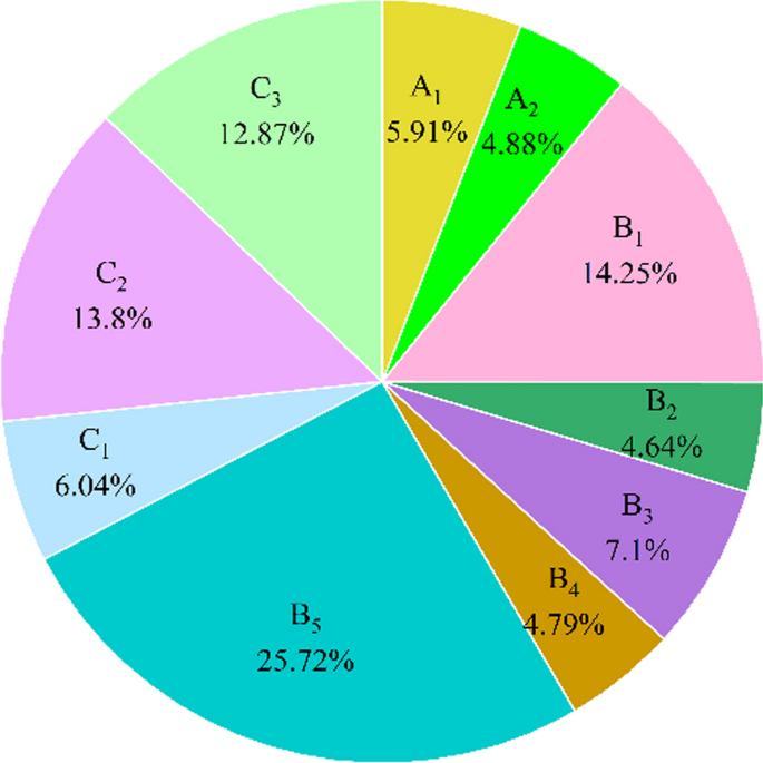
Objective weight calculation results

-
(2)
Determination of subjective weight by the AHP.
According to the rockburst risk evaluation indicator system shown in Fig. 1, we invited three mining engineering experts and two geotechnical engineering experts to conduct subjective scoring. Establish the judgment matrix in Eq. (8) by averaging their scores, and use Eq. (10) to check consistency. Finally, the relative calculation weight results of the indicator layer and the target layer are obtained by using Eq. (11), as shown in Fig. 4.
Fig. 4 
Subjective weight calculation results
-
(3)
Determination of combination weights.
The combined weight of each evaluation indicator can be calculated using Eq. (3) in the combined weighting method, as shown in Fig. 5.
Fig. 5 
Combined weight calculation results
As can be seen from Fig. 5, the order of the importance of each evaluation indicator in the criterion layer is: C > B > A, and the importance of each evaluation indicator in the indicator layer is: C2 > C1 > C3, B5 > B1 > B3 > B2 > B4, A1 > A2.
-
(3)


3.4 Calculation of catastrophe level value
From Fig. 1, it can be observed that the indicator layer An to the criterion layer A, the indication layer Bn to the criterion layer B, the indicator layer Cn to the criterion layer C, and the criterion layer to the target layer conform to the cusp catastrophe model, the Indian hut catastrophe model, the swallowtail catastrophe model, and the swallowtail catastrophe model, respectively, in the common catastrophe model presented in Table 1. Therefore, according to the importance order of each evaluation indicator determined in Sect. 3.3, it is substituted into the normalized formula of the catastrophe model in Table 1 for calculation. Moreover, the selected rockburst risk assessment indicators in this paper exhibit a strong correlation, satisfying the principle of complementarity. Therefore, the “average value” method is used to calculate the normalized value of the system. The calculation results are shown in Table 4.
3.5 Relationship between rockburst level and catastrophe level
Figure 6 shows the catastrophe level values calculated in Table 4 and the rockburst identification level of each sample.

Relationship between rockburst level and catastrophe level value
As can be seen from Fig. 6, the larger the catastrophe level, the higher the rockburst level. The catastrophe level value based on the combined weighting catastrophe progression model has a good positive correlation with the rockburst level, with clear differences between levels. Therefore, the catastrophe level value can be used as a new standard for assessing the rockburst level. Based on the observation in Fig. 6, the catastrophe level can be divided into intervals to represent the rockburst level. The no impact propensity is represented by X < 0.75, the weak impact propensity is represented by 0.75 ≤ X < 0.85, and the strong impact propensity is represented by X ≥ 0.85.
3.6 Validation analysis and comparison
The calculated catastrophe level values for the 10 samples in this work are used to determine the rockburst level by comparing them to the division intervals. The results are then compared to the risk assessment made using the unimproved catastrophe progression method and the single indicator risk assessment method, which includes uniaxial compressive strength, impact energy indicator, and bending energy indicator. The classification criteria for rockburst levels in the single indicator risk assessment method are mainly based on the classification and evaluation criteria in national standards such as "Standard for the Determination of Coal Seam Burst Tendency" and "Standard for the Determination of Rockburst Tendency", as shown in Table 5. The results of this analysis are presented in Table 6.
As shown in Table 6, when the catastrophe level values calculated by the improved combined weighting catastrophe progression method for sample data are substituted to the rockburst intensity level, the rockburst results assessed for all 10 samples are consistent with the rockburst propensity identification results, achieving a risk assessment accuracy of 100%. However, in the single indicator risk assessment method, the risk assessment accuracy of the results obtained based on the uniaxial compressive strength, impact energy indicator, and bending energy indicator are 90, 80, and 70%, respectively. The accuracy of the risk assessment results using the unimproved catastrophe progression method is 70%. Therefore, the combined weighting catastrophe progression method model established in this paper is accurate and reliable for assessing rockburst intensity level.
4 Discussion
The risk assessment results of different methods show that the accuracy of the risk assessment results obtained from uniaxial compressive strength in the single indicator risk assessment method is up to 90%. Moreover, through comparing and analyzing the uniaxial compressive strength in the original data with the catastrophe level values obtained from the model in the paper, it can be concluded that the variation trend of the uniaxial compressive strength and the catastrophe levels is highly similar (except for individual cases, such as sample 5), as shown in Fig. 7. Therefore, it can be considered that uniaxial compressive strength plays an important role in assessing the propensity for rockburst in coal mines. Reducing the uniaxial compressive strength of coal can effectively prevent the occurrence of rockburst, which is consistent with the research results of many scholars who have reduced the strength of coal seams by means of water injection (Liu et al. 2021) and microwave radiation (Guozhong et al. 2021). This further verifies the feasibility and accuracy of the rockburst risk assessment model.

Relationship between uniaxial compressive strength and catastrophe level
In this paper, a risk assessment model for rockburst based on combined weighting catastrophe progression method is established and applied to an engineering example, which is verified to be feasible and effective. However, due to the complexity of rockburst and numerous influencing factors, although the risk assessment model selects 10 key indicators of three influencing factors, namely, in-situ stress distribution, geological conditions, and mechanical properties, for analysis, the conditions for occurrence of rockburst in practical projects are far more complex and involve various evaluation indicators. Furthermore, there is also a coupling effect between various evaluation indicators. Therefore, to assess the intensity level of rockburst more scientifically and accurately, it is also necessary to improve the selection of evaluation indicators for the impact factors of rockburst, so as to continuously optimize the risk assessment indicator system and the calculation method of weight. In addition, while the model has been applied and verified in this case, its applicability to other cases needs to be verified.
5 Conclusions
In this paper, ten main factors affecting rockburst are selected to develop an evaluation indicator system for rockburst risk assessment based on the combined weighting method and catastrophe progression method. Subsequently, this model is applied to engineering practice. The following conclusions can be drawn from this study.
-
(1)
Based on selecting 8 commonly used indicators such as maximum principal stress, coal seam burial depth, inclination angle, complexity, thickness, uniaxial compressive strength, impact energy index, and roof bending energy index, and considering the minimum principal stress and coefficient of variation that are not commonly used but have a large influence on rockburst, they are collectively used as the main evaluation indicators for assessing rockburst, making the evaluation index system more comprehensive.
-
(2)
The combined weighting method of objective weighting of variation coefficient and subjective weighting of the analytic hierarchy process is used to weight each evaluation indicator determine the relative importance of each indicator at the indicator layer and criterion layer, which can effectively avoid the problem of absoluteness and subjectivity in the process of traditional weight distribution.
-
(3)
By applying the evaluation indicator data of 10 mines to the rockburst risk assessment model based on the combined weighting catastrophe progression method and comparing it with the risk assessment results from the unimproved catastrophe progression method, the accuracy of the risk assessment is improved by 42.85%. Therefore, it can be concluded that the risk assessment model established in this paper is both accurate and reliable.
-
(4)
According to the comparative analysis between the model risk assessment results and the original indicators, it is concluded that the intensity level of coal mine rockburst can be reduced by decreasing the uniaxial compressive strength of the coal seam. This finding confirms the research results of other scholars and verifies the accuracy of the model once again.
Data availability
The datasets generated and analyzed during the current study are available from the corresponding author on reasonable request.
References
Cai W, Bai X, Si G, Cao W, Gong S, Dou L (2020) A monitoring investigation into rock burst mechanism based on the coupled theory of static and dynamic stresses. Rock Mech Rock Eng 53(12):5451. https://doi.org/10.1007/s00603-020-02237-6
Chen L, Gao X, Gong S, Li Z (2020) Regionalization of green building development in china: a comprehensive evaluation model based on the catastrophe progression method. Sustainability 12(15):5988. https://doi.org/10.3390/su12155988
Chen J, Zhu C, Du J, Pu Y, Pan P, Bai J, Qi Q (2022) A quantitative pre-warning for coal burst hazardous zones in a deep coal mine based on the spatio-temporal forecast of microseismic events. Process Safety Environ Protect 159(1105). https://doi.org/10.1016/j.psep.2022.01.082
Du J, Chen J, Pu Y, Jiang D, Chen L, Zhang Y (2021). Risk assessment of dynamic disasters in deep coal mines based on multi-source, multi-parameter indexes, and engineering application. Process Safety Environ Protect 155(575). https://doi.org/10.1016/j.psep.2021.09.034
Feng G, Xia G, Chen B, Xiao Y, Zhou R (2019) A method for rockburst risk assessment in the deep tunnels of hydropower stations based on the monitored microseismicity and an optimized probabilistic neural network model. Sustainability 11(11):3212. https://doi.org/10.3390/su11113212
Gao M, Song Z, Duan H, Xin H, Tang J (2020) Mechanical properties and control rockburst mechanism of coal and rock mass with bursting liability in deep mining. Shock Vibrat 2020(1). https://doi.org/10.1155/2020/8833863
Ghasemi E, Gholizadeh H, Adoko AC (2020) Evaluation of rockburst occurrence and intensity in underground structures using decision tree approach. Eng Comp 36(1):213. https://doi.org/10.1007/s00366-018-00695-9
Guozhong Hu, Chunbo W, Jialin Xu, Xufei Wu, Wei Q (2021) Experimental investigation on decreasing burst tendency of hard coal using microwave irradiation. J China Coal Soc 46(2):450. https://doi.org/10.13225/j.cnki.jccs.XR20.1906
He Z, Lu C, Zhang X, Guo Y, Wang C, Zhang H, Wang B (2022) Research on mechanisms and precursors of slip and fracture of coal-rock parting-coal structure. Rock Mech Rock Eng 55(3):1343. https://doi.org/10.1007/s00603-021-02724-4
He M, Zhang Z, Zhu J, Li N, Li G, Chen Y (2021) Correlation between the rockburst proneness and friction characteristics of rock materials and a new method for rockburst proneness risk assessment: field demonstration. J Petrol Sci Eng 205(108997). https://doi.org/10.1016/j.petrol.2021.108997
He S, Song D, Mitri H, He X, Chen J, Li Z, Xue Y, Chen T (2021) Integrated rockburst early warning model based on fuzzy comprehensive evaluation method. Int J Rock Mech Mining Sci 142(104767). https://doi.org/10.1016/j.ijrmms.2021.104767
Hou WT, Wang HP, Yuan L, Wang W, Xue Y, Ma ZW (2021) Experimental research into the effect of gas pressure, particle size and nozzle area on initial gas-release energy during gas desorption. Int J Min Sci Technol 31(2):253. https://doi.org/10.1016/j.ijmst.2021.01.002
Jin P, Wang E, Huang N, Wang S (2013) Catastrophe progression method on forecast of rock burst. Disas Adv, 2.
Li L (2020) Rockburst grade evaluation based on improved catastrophe progression method. Hebei University of Engineering
Li CC, Mikula P, Simser B, Hebblewhite B, Joughin W, Feng X, Xu N (2019) Discussions on rockburst and dynamic ground support in deep mines. J Rock Mech Geotechnical Eng 11(5):1110. https://doi.org/10.1016/j.jrmge.2019.06.001
Liu N, Li C, Feng R, Xia X, Gao X (2021) Experimental study of the influence of moisture content on the mechanical properties and energy storage characteristics of coal. Geofluids 2021(1). https://doi.org/10.1155/2021/6838092
Ma T, Tang C, Tang S, Kuang L, Yu Q, Kong D, Zhu X (2018) Rockburst mechanism and risk assessment based on microseismic monitoring. Int J Rock Mech Mining Sci 110(177). https://doi.org/10.1016/j.ijrmms.2018.07.016
Mi C, Zuo J, Sun Y, Zhao S (2022) Investigation on rockburst mechanism due to inclined coal seam combined mining and its control by reducing stress concentration. Nat Resour Res 31(6):3341. https://doi.org/10.1007/s11053-022-10118-8
Miao S, Cai M, Guo Q, Huang Z (2016) Rock burst risk assessment based on in-situ stress and energy accumulation theory. Int J Rock Mech Mining Sci 83(86). https://doi.org/10.1016/j.ijrmms.2016.01.001
Ranjith PG, Zhao J, Ju M, De Silva RVS, Rathnaweera TD, Bandara AKMS (2017) Opportunities and challenges in deep mining: a brief review. Engineering 3(4):546. https://doi.org/10.1016/J.ENG.2017.04.024
Senan CPC, Ajin RS, Danumah JH, Costache R, Arabameri A, Rajaneesh A, Sajinkumar KS, Kuriakose SL (2023) Flood vulnerability of a few areas in the foothills of the Western Ghats: a comparison of AHP and F-AHP models. Stoch Env Res Risk Assess 37(2):527. https://doi.org/10.1007/s00477-022-02267-2
Singh LK, Jha MK, Chowdary VM (2022) Application of catastrophe theory to spatial analysis of groundwater potential in a sub-humid tropical region: a hybrid approach. Geocarto Int 37(3):700. https://doi.org/10.1080/10106049.2020.1737970
Stas L, Soucek K, Knejzlik J (2007) First results of conical borehole strain gauge probes applied to induced rock mass stress changes measurement. Acta Geodyn Et Geomater 4(4):77
State Administration of Coal Mine Safety Implementation Rules for the Prevention and Control of Coal Mine Rockburst, China Coal Industry Publishing House,2018
Tang LZ, Xia KW (2010) Seismological method for risk assessment of areal rockbursts in deep mine with seismic source mechanism and unstable failure theory. J Cent South Univ Technol 17(5):947. https://doi.org/10.1007/s11771-010-0582-5
Wang K, Du F (2020). Coal-gas compound dynamic disasters in China: a review. Proc Saf Environ Prot 133(1). https://doi.org/10.1016/j.psep.2019.10.006
Wang C, Wu A, Lu H, Bao T, Liu X (2015) Assessing rockburst tendency based on fuzzy matter-element model. Int J Rock Mech Mining Sci 75(224). https://doi.org/10.1016/j.ijrmms.2015.02.004
Wang M W, Liu Q Y, Wang X, Shen F Q, Jin J L (2020). Risk assessment of Rockburst Based on Multidimensional Connection Cloud Model and Set Pair Analysis Int J Geomech 20(1). https://doi.org/10.1061/(ASCE)GM.1943-5622.0001546
Wang W, Wang H, Zhang B, Wang S, Xing W (2021) Coal and gas outburst risk assessment model based on extension theory and its application. Proc Saf Environ Prot 154(329). https://doi.org/10.1016/j.psep.2021.08.023
Wang H, Zhang B, Yuan L, Wang S, Yu G, Liu Z (2022) Analysis of precursor information for coal and gas outbursts induced by roadway tunneling: a simulation test study for the whole process. Tunnell Underground Space Technol 122(104349). https://doi.org/10.1016/j.tust.2021.104349
Wei C, Zhang C, Canbulat I, Cao A, Dou L (2018) Evaluation of current coal burst control techniques and development of a coal burst management framework. Tunnell Underground Space Technol 81(129). https://doi.org/10.1016/j.tust.2018.07.008
Xia G, Luan T, Sun M (2017) An evaluation method for sortie generation capacity of carrier aircrafts with principal component reduction and catastrophe progression method. Math Problems Eng 2017(1). https://doi.org/10.1155/2017/2678216
Xu C, Liu X, Wang E, Zheng Y, Wang S (2018). Rockburst risk assessment and classification based on the ideal-point method of information theory. Tunnell Underground Space Technol 81(382). https://doi.org/10.1016/j.tust.2018.07.014
Xue Y, Bai C, Qiu D, Kong F, Li Z (2020). Assessing rockburst with database using particle swarm optimization and extreme learning machine. Tunnell Underground Space Technol 98(103287). https://doi.org/10.1016/j.tust.2020.103287
Xue R, Liang Z, Xu N (2021). Rockburst risk assessment and analysis of activity characteristics within surrounding rock based on microseismic monitoring and numerical simulation. Int J Rock Mech Mining Sci 142(104750). https://doi.org/10.1016/j.ijrmms.2021.104750
Yin X, Liu Q, Pan Y, Huang X, Wu J, Wang X (2021) Strength of stacking technique of ensemble learning in rockburst risk assessment with imbalanced data: comparison of eight single and ensemble models. Nat Resour Res 30(2):1795. https://doi.org/10.1007/s11053-020-09787-0
Zhai S, Su G, Yin S, Yan S, Wang Z, Yan L (2020) Fracture evolution during rockburst under true-triaxial loading using acoustic emission monitoring. Bull Eng Geol Env 79(9):4957. https://doi.org/10.1007/s10064-020-01858-z
Zhang L, Zhang X, Wu J, Zhao D, Fu H (2020) Rockburst risk assessment model based on comprehensive weight and extension methods and its engineering application. Bull Eng Geol Env 79(9):4891. https://doi.org/10.1007/s10064-020-01861-4
Zhang H, Zeng J, Ma J, Fang Y, Ma C, Yao Z, Chen Z (2021a) Time series risk assessment of microseismic multi-parameter related to rockburst based on deep learning. Rock Mech Rock Eng 54(12):6299. https://doi.org/10.1007/s00603-021-02614-9
Zhang Q, Wang E, Feng X, Wang C, Qiu L, Wang H (2021b) Assessment of rockburst risk in deep mining: an improved comprehensive index method. Nat Resour Res 30(2):1817. https://doi.org/10.1007/s11053-020-09795-0
Zhang B, Wang H, Wang P, Yu G, Gu S (2023) Experimental and theoretical study on the dynamic effective stress of loaded gassy coal during gas release. Int J Min Sci Technol 33(3):339. https://doi.org/10.1016/j.ijmst.2022.09.025
Zheng Y, Zhong H, Fang Y, Zhang W, Liu K, Fang J (2019) Rockburst risk assessment model based on entropy weight integrated with grey relational BP neural network. Adv Civil Eng 2019(1). https://doi.org/10.1155/2019/3453614
Acknowledgements
This work was supported by the National Natural Science Foundation of China (Grant No. 52227901; Grant No. 52174081).
Funding
This work was supported by the National Natural Science Foundation of China (Grant No. 52227901; Grant No. 52174081).
Author information
Authors and Affiliations
Contributions
WX: conceptualization, methodology, investigation, writing—original draft. HW: conceptualization, funding acquisition, resources, supervision, writing—review & editing. JF: investigation, data collection and analysis. WW: investigation, data analysis and interpretation. XY: investigation, data processing.
Corresponding author
Ethics declarations
Conflict of Interest
The authors declare that they have no known competing financial interests or personal relationships that could have appeared to influence the work reported in this paper.
Additional information
Publisher's Note
Springer Nature remains neutral with regard to jurisdictional claims in published maps and institutional affiliations.
Rights and permissions
Springer Nature or its licensor (e.g. a society or other partner) holds exclusive rights to this article under a publishing agreement with the author(s) or other rightsholder(s); author self-archiving of the accepted manuscript version of this article is solely governed by the terms of such publishing agreement and applicable law.
About this article

Cite this article
Xing, W., Wang, H., Fan, J. et al. Rockburst risk assessment model based on improved catastrophe progression method and its application. Stoch Environ Res Risk Assess 38, 981–992 (2024). https://doi.org/10.1007/s00477-023-02609-8
Accepted:
Published:
Issue Date:
DOI: https://doi.org/10.1007/s00477-023-02609-8