
Abstract
This work focuses on elucidating issues related to an increasingly common technique of multi-model ensemble (MME) forecasting. The MME approach is aimed at improving the statistical accuracy of imperfect time-dependent predictions by combining information from a collection of reduced-order dynamical models. Despite some operational evidence in support of the MME strategy for mitigating the prediction error, the mathematical framework justifying this approach has been lacking. Here, this problem is considered within a probabilistic/stochastic framework which exploits tools from information theory to derive a set of criteria for improving probabilistic MME predictions relative to single-model predictions. The emphasis is on a systematic understanding of the benefits and limitations associated with the MME approach, on uncertainty quantification, and on the development of practical design principles for constructing an MME with improved predictive performance. The conditions for prediction improvement via the MME approach stem from the convexity of the relative entropy which is used here as a measure of the lack of information in the imperfect models relative to the resolved characteristics of the truth dynamics. It is also shown how practical guidelines for MME prediction improvement can be implemented in the context of forced response predictions from equilibrium with the help of the linear response theory utilizing the fluctuation–dissipation formulas at the unperturbed equilibrium. The general theoretical results are illustrated using exactly solvable stochastic non-Gaussian test models.
1 Introduction
Dynamical prediction of complex multi-scale systems based on imperfect models and spatiotemporally sparse observations of the truth dynamics is a notoriously difficult problem which is, nevertheless, essential in many applications such as climate-atmosphere science (Emanuel et al. 2005; Randall 2007), materials science (Chatterjee and Vlachos 2007; Katsoulakis et al. 2003), neuroscience (Rangan et al. 2009), or systems biology and biochemistry (Noé et al. 2009; Sriraman et al. 2005; Das et al. 2006; Hummer and Kevrekidis 2003). Due to the high-dimensional, multi-scale nature of such time-dependent problems, it is challenging to obtain even statistically accurate predictions of the coarse-grained characteristics of the truth dynamics. Advances in computing power and new theoretical insights have spurred the development of a plethora of reduced-order models (e.g., Epstein 1969; Emanuel et al. 2005; Neelin et al. 2006; Randall 2007; Sapsis and Majda 2013d; Chen et al. 2014a; Thual et al. 2014) and data assimilation techniques (e.g., Anderson 2007; Houtekamer and Mitchell 2001; Harlim and Majda 2010; Gershgorin et al. 2010a; Majda and Harlim 2012; Majda et al. 2014; Grooms et al. 2014; Chen et al. 2014b). Various ways of minimizing uncertainties in imperfect predictions and validating reduced-order models have been developed in this context (e.g., Majda and Gershgorin 2010, 2011a, b; Branicki and Majda 2012c, 2014; Majda and Branicki 2012c). Data assimilation aside, one of the most important challenges in improving imperfect dynamical predictions concerns the mitigation of model error. Recent developments provide new techniques for mitigating coarse-graining errors, and for counteracting errors due to neglecting nonlinear interactions between the resolved and unresolved processes in reduced-order models; these include the stochastic superparameterization (Grooms and Majda 2013, 2014; Majda and Grooms 2014; Grooms et al. 2015; Slawinska et al. 2015) and reduced subspace closure techniques (Sapsis and Majda 2013a, b, c).
This work focuses on elucidating issues related to an increasingly common technique of multi-model ensemble (MME) predictions which is complementary to improving individual imperfect models. The heuristic idea behind MME prediction is simple: Given a collection of imperfect models, consider the prediction obtained through a linear superposition of individual model forecasts in the hope of mitigating the overall prediction error. While there is some evidence in support of the MME approach for improving imperfect predictions, particularly in atmospheric sciences (e.g., Palmer et al. 2005; Stephenson et al. 2005; Doblas-Reyes et al. 2005; Hagedorn et al. 2005; Weigel et al. 2008; Weisheimer et al. 2009; van der Linden and Mitchell 2009; Oldenborgh et al. 2012), a systematic framework justifying this approach has been lacking. In particular, it is not obvious which imperfect models, and with what weights, should be included in the MME forecast in order to improve predictions within this framework. Consequently, virtually all operational MME prediction systems for weather and climate are based on equal-weight ensembles (Hagedorn et al. 2005; Weigel et al. 2008; van der Linden and Mitchell 2009; Weisheimer et al. 2009; Oldenborgh et al. 2012) which are likely to be far from optimal (Doblas-Reyes et al. 2005) in the absence of additional restrictions imposed on the ensemble members. Our main focus is on a systematic understanding of benefits and limitations associated with the MME approach to improving imperfect predictions; important practical issues in this context are the following:
-
(a)
How to measure the skill (statistical accuracy) of dynamic MME predictions relative to single-model predictions? (This setting should not be confused with a purely statistical modeling in which the underlying dynamics is ignored.)
-
(b)
Is there a condition guaranteeing an improvement in predictions via the MME approach relative to single-model predictions?
We consider the MME prediction within a probabilistic/stochastic framework which exploits tools from information theory in order to systematically understand the characteristics of such an approach. This probabilistic framework can be utilized in two different contexts: First, when dealing with deterministic imperfect models, one can consider a time-dependent probability density function constructed by initializing the models from a given distribution of initial conditions. Second, the probabilistic prediction framework arises naturally when using stochastic reduced-order models in imperfect predictions which is an increasingly common approach (e.g., Epstein 1969; Lorenz 1968, 1969; Palmer 2001; Palmer et al. 2005; Majda et al. 2005; Majda and Wang 2010; Sapsis and Majda 2013d; Chen et al. 2014a; Thual et al. 2014). In many operational situations, dynamic predictions can be obtained through a weighted superposition of forecasts obtained from a collection of imperfect models (e.g., Hagedorn et al. 2005; Weigel et al. 2008; van der Linden and Mitchell 2009; Weisheimer et al. 2009; Oldenborgh et al. 2012). However, the individual imperfect models are usually highly complex and not easily tuneable, and it is desirable to consider the possibility of prediction improvement by adjusting only the ensemble weights. In order to shed light on the issues (a)–(b) above, we set out an information-theoretic framework capable of
-
(i)
Quantification of uncertainty and improving the imperfect predictions via the MME approach;
-
(ii)
Providing practical guidelines for improving dynamic MME predictions given a small collection of available imperfect models.
Here, we derive a simple criterion for improving probabilistic predictions via the MME approach. Moreover, we provide a simple justification of why the MME prediction can have a better prediction skill than the best single model in the ensemble. Finally, we derive systematic guidelines for constructing finite model ensembles which are likely to have a superior predictive skill over any single model in the ensemble. These results stem largely from the convexity of the relative entropy (e.g., Cover and Thomas 2006) which is used here as a measure of the lack of information in the imperfect models relative to the resolved characteristics of the truth dynamics. We show that the guidelines for MME prediction improvement in the context of a forced perturbation from an equilibrium can be implemented with the help of the linear response theory and the ‘fluctuation–dissipation’ approach for forced dissipative systems (Majda et al. 2005, 2010b, a; Leith 1975; Abramov and Majda 2007; Gritsun et al. 2008; Majda and Gershgorin 2011b); this approach follows from the earlier work on improving imperfect predictions in the presence of model error in the single-model setup (see for example, Kleeman 2002; Majda et al. 2002; Kleeman et al. 2002; Majda and Gershgorin 2010, 2011a, b; Gershgorin and Majda 2012; Branicki and Majda 2012c; Majda and Branicki 2012c). When considering prediction improvement for the initial value problem, the practical implementation of the condition for skill improvement through MME can be carried out in the hindcast/reanalysis mode (e.g., Kim et al. 2012). Although we focus here on mitigating the prediction error via the MME approach, it is worth stressing that the ultimate goal in imperfect reduced-order prediction should involve a synergistic approach that combines the improvement in reduced-order models with an MME framework for both data assimilation and prediction.
This paper is structured as follows: First, in Sect. 2, we motivate the need for a systematic analysis of the MME prediction problem. In Sect. 3, we derive the information-theoretic criterion for improving MME predictions relative to single-model predictions. A set of particularly useful results is discussed in Sect. 3.2 where Gaussian models are used in a MME; this approach provides a helpful intuition for dealing with the general results of Sect. 3. Section 4 combines the analytical estimates of Sect. 3 with simple numerical tests which are based on statistically exactly solvable models described in Sect. 4.1. We conclude in Sect. 5 by summarizing the most important results, and we discuss directions for further research in this area, including extensions of the MME approach to improving imperfect data assimilation techniques. Technical details associated with the analytical estimates derived in Sect. 3 are presented in the appendices.
2 Motivating Examples
Consider the dynamics of a high-dimensional, nonlinear system where only a small subset of its dynamical variables can be reasonably modeled or accessed through empirical measurements. The resolved dynamics of the full system is affected by nonlinear, multi-scale interactions with unresolved processes which cannot be observed or even correctly modeled (e.g., Majda and Wang 2006). Nevertheless, we are interested in a statistically accurate prediction of the resolved non-equilibrium dynamics using a collection of imperfect reduced-order dynamical models which approximate or neglect the interactions between the resolved and unresolved processes. To this end, assume that the state vector of dynamical variables in the true high-dimensional system decomposes as \(\mathbf{v}=(\pmb {u},\pmb {v})\), where \(\pmb {u}\in {\mathbb {R}}^K, K<\infty \), denotes the resolved variables and \(\pmb {v}\in {\mathbb {R}}^N\) denotes the unresolved variables; we tacitly assume that \(K\ll N\) which is natural when dealing with complex multi-scale dynamics such as the turbulent dynamics of geophysical flows (e.g., Majda and Wang 2006). The time-dependent probability density associated with the MME of imperfect reduced-order models on the subspace of the resolved variables \(\pmb {u}\) is given by a convex superposition of the model densities in the form
where \(\pi ^{{\textsc {m}}_i}_t\) represents probability densities associated with the imperfect models \({\textsc {m}}_i\) in some class \({\mathcal {M}}\). We are particularly interested in mitigating the MME prediction error by adjusting the model weights \(\alpha _i\) in (1) with fixed characteristics of the individual imperfect models \({\textsc {m}}_i\in {\mathcal {M}}\) which is desirable from the practical viewpoint. The lack of information at time \(t\) between the MME and the truth statistics on the resolved subspace of variables is measured using the relative entropy (Kullback and Leibler 1951) given by
This nonnegative functional satisfying \({\mathcal {P}}(\pi _t,\pi ^{{\textsc {mme}}}_{\pmb {\alpha },t})= 0\) only when \(\pi _t=\pi ^{{\textsc {mme}}}_{\pmb {\alpha },t}\) is not a proper metric. However, it possesses a number of desirable properties such as convexity in the pair \((\pi ,\pi ^{{\textsc {mme}}})\), and it satisfies a ‘triangle equality’ for a certain class of densities discussed later (see also Majda et al. 2005; Branicki and Majda 2012c; Majda and Branicki 2012c); moreover, the relative entropy is invariant under general changes in variables (Majda et al. 2002; Majda and Wang 2006) [i.e., (2) can be written in a form which is independent of the dominating measure which we skip here but see, e.g., Gibbs and Su 2002]. We use the relative entropy (2) as an information-based measure of the time-dependent error in the imperfect probabilistic predictions; additional measures of predictive skill were introduced earlier in the context of uncertainty quantification in the single-model context and are briefly discussed in Sect. 4.3.1 (see also Majda and Gershgorin 2011a, b; Majda and Wang 2010; Branicki and Majda 2012c; Majda and Branicki 2012c). Here, we show that the information-theoretic approach is very useful when considering prediction improvement in the MME context. In particular, this setting helps address the following general questions:
-
What characteristics of the model ensemble lead to uncertainty reduction in MME predictions relative to imperfect predictions with a single model?
In the subsequent sections, we derive a set of information criteria for improving probabilistic dynamical predictions via the MME approach relative to the best single imperfect model. However, before embarking on a detailed analysis, some motivating examples are presented in Fig. 1 which shows that: (i) not every MME prediction is superior to the single-model prediction and (ii) the structure of the optimal-weight MME depends on both the truth dynamics and the imperfect models in the ensemble. The top-row insets show the evolution of the prediction error in terms of the relative entropy (2) in three different dynamical regimes of a non-Gaussian truth dynamics (described later in Sect. 4.1.2). In all cases, the statistics of the initial conditions and the marginal equilibrium for the resolved dynamics in the imperfect Gaussian models \({\textsc {m}}_i\) coincide with those of the truth dynamics; in addition, the single-model predictions are carried out with an imperfect model tuned to have the correct correlation time \(\tau ^\mathrm{trth}\) of the resolved dynamics at equilibrium. The bottom row in Fig. 1 shows the weight structure of the MME with individual models in the ensemble labeled by the correlation time \(\tau \) of their equilibrium dynamics; the optimal-weight MME is obtained in this case by minimizing the average relative entropy \(\frac{1}{T}\!\int _0^T\!{\mathcal {P}}(\pi _t,\pi ^{{\textsc {mme}}}_t){\mathrm{d}}t\) over the whole time interval considered. Note that the error of the MME prediction relative to the single-model prediction varies significantly between the three configurations in Fig. 1a–c; moreover, the structure of the optimal-weight MME changes drastically from an MME containing only models with \(\tau ^{{\textsc {m}}_i}>\tau ^\mathrm{trth}\) in (a), to an MME with \(\tau ^{{\textsc {m}}_i}<\tau ^\mathrm{trth}\) in (b), to an MME containing a single imperfect model with the shortest correlation time in the ensemble in (c). The difference between the configuration in (a) and (b) lies in the initial statistical conditions: In (a), the initial conditions are such that the resolved dynamics is in a stable regime, while in (b), the resolved dynamics is initially in a transient unstable phase. The configuration shown in Fig. 1c corresponds to imperfect predictions of the resolved non-Gaussian dynamics when the truth equilibrium statistics is significantly skewed. (See Sect. 4.3.2 for more details.)

Dependence of the prediction error within the MME framework on the nature of the non-Gaussian truth dynamics [given by (38) in Sect. 4.1.2]; here, the MME mixture density (1) contains Gaussian models (26) with correct statistics of the initial conditions and correct marginal equilibrium for the resolved dynamics. Top-row insets show the evolution of the error via the relative entropy (2) for predicting the resolved truth dynamics with: (left) symmetric fat-tailed equilibrium density with initial statistical conditions in a stable regime of the truth dynamics, (middle) symmetric fat-tailed equilibrium density with initial conditions in an unstable regime of the truth, and (right) skewed equilibrium density with initial conditions in a stable regime of the truth. The bottom insets show the weights \(\alpha _i\) in MME density (1); the optimal-weight MME (9) minimizes the time-averaged relative entropy by adjusting the ensemble weights. Note that the performance of MME prediction, as well as the structure of the optimal-weight MME, depends strongly on the nature of the truth dynamics
Clearly, the performance of the MME approach for improving imperfect predictions depends on both the structure of the MME and the nature of the truth dynamics. The above examples highlight the need for a more analytical insight which would allow to understand when and why the MME approach leads to improved predictions. In the next section, we focus solely on this topic and we obtain information-based criteria for prediction improvement via the MME approach. The general theoretical results derived in Sect. 3 are discussed further in Sect. 4 based on two simple but revealing test models described in Sect. 4.1.
3 Information-Theoretic Criteria for Improving MME Predictions
Here, we develop an information-theoretic framework for assessing the potential improvement in imperfect predictions through the MME approach. First, in Sect. 3.1, we derive a condition for improving the predictive skill within the MME framework; this condition requires evaluating certain least-biased estimates of the truth which are obtained by maximizing the Shannon entropy subject to a finite number of moment constraints, making this approach amenable to applications. Implications of this information-based criterion are discussed in Sect. 3.1.3 for both the initial value problem and the forced response prediction. Further insight and intuition can be gained by restricting the MME prediction problem to the Gaussian mixture configuration which is discussed in Sect. 3.2. The results presented here exploit the convexity of the relative entropy (2) between the truth and the MME density in (1) which measures the lack of information in the MME density relative to the resolved truth statistics. Further details, along with some simple proofs of the facts established below, are relegated to “Appendix 1”.
3.1 Improving Predictions Through MME Framework
Consider imperfect probabilistic predictions of the truth dynamics on the subspace of resolved variables \(\pmb {u}\in {\mathbb {R}}^K\) based on the MME with density \(\pi ^{{\textsc {mme}}}_{\pmb {\alpha },t}\) in (1). As in Sect. 2, we assume that the truth dynamics has the probability density function denoted by \(p_t({\pmb {u},\pmb {v}}),\,\pmb {v}\,{\in }\,{\mathbb {R}}^N,\;K{\ll }\,N\), and the corresponding marginal density on the resolved subspace is \(\pi _t(\pmb {u})=\int \!p_t(\pmb {u},\pmb {v}){\mathrm{d}}\pmb {v}\). Given some class \({\mathcal {M}}\) of reduced-order models for the resolved dynamics \(\pmb {u}(t)\), we define the best single model \({\textsc {m}}_*\) for making predictions at time \(t \) as the one with the smallest error in terms of the relative entropy
where \(\pi _t\) is the truth density, \(\pi ^{{\textsc {m}}}_t\) represents the probability density associated with the models \({\textsc {m}}\in {\mathcal {M}}\), and the relative entropy \({\mathcal {P}}(\pi _t,\pi ^{{\textsc {m}}}_t)\) measures the lack of information in \(\pi ^{{\textsc {m}}}_t\) relative to the truth marginal density \(\pi _t\) (see Majda and Gershgorin 2010, 2011a, b; Branicki and Majda 2012c; Majda and Branicki 2012c). Analogously, the best single model \({\textsc {m}}_{{\mathcal {I}}}^*\in {\mathcal {M}}\) for making predictions over the time interval \( {\mathcal {I}}\) is given by
where  measures the average lack of information over the time interval \({\mathcal {I}}\). We introduce the following information measures to quantify the performance of the MME prediction relative to the single-model prediction with model

where  denotes the integral average over the time interval \({\mathcal {I}}\), and \(\pi ^{\textsc {l}}\) in (5b) is the least-biased estimate of the truth density which maximizes the Shannon entropy subject to \({\textsc {l}}\) moment constraints (see (14) below and Mead and Papanicolaou (1984); Majda et al. (2005); Majda and Gershgorin (2011a, b); Branicki and Majda (2012c)). Importantly, the two measures in (5) have a common upper bound
if ensemble models in \(\mathcal {M}\) have the least-biased structure \({\textsc {m}}_i={\textsc {m}}_i^{{\textsc {l}}'}, {\textsc {l}}'\leqslant {\textsc {l}}\) (see (14) in §3.1.1); this fact stems from the convexity of the relative entropy (10) and the ‘triangle equality’ (11) satisfied by \(\mathcal {P_{\mathcal {I}}}\) which are discussed below. While the measure \(\mathfrak {P}^{\textsc {mme},{\textsc {m}}_{\diamond }}_{\pmb {\alpha },\mathcal {M},{\mathcal {I}}}\) is the most appropriate one, it is unrealistic to expect that it can be evaluated in practice since the exact truth density, \(\pi \), is unlikely to be known. On the other hand, the use of the least-biased estimate, \(\pi ^{\textsc {l}}\), of the truth density represents a practically achievable approach. Thus, we adopt the following:
Information Criterion I The MME prediction utilizing models \({\textsc {m}}\in {\mathcal {M}}\) with weights \(\pmb {\alpha }\) over the time interval \({\mathcal {I}}\) has a smaller error than the single model prediction with \({\textsc {m}}_{\diamond }\) if
Note that the single model \({\textsc {m}}_{\diamond }\) in (5) and (7) does not have to coincide with the best imperfect model \({\textsc {m}}^*_{\mathcal {I}}\) in (4) which is unknown in practice. For example, one might consider \({\textsc {m}}_{\diamond }\) to be the best single model \({\textsc {m}}_{{\mathcal {I}},{\textsc {l}}}^*\) relative to the least-biased truth estimate which is defined as
and it clearly depends on the \({\textsc {l}}\) moment constraints used to estimate the truth density. Note that even if \({\mathcal {P}}_{\mathcal {I}}(\pi ^{\textsc {l}},\pi ^{{\textsc {m}}_{{\mathcal {I}},{\textsc {l}}}^*})=0\), there might exist an information barrier \({\mathcal {P}}_{\mathcal {I}}(\pi ,\pi ^{{\textsc {m}}_{{\mathcal {I}},{\textsc {l}}}^*}) = {\mathcal {P}}_{\mathcal {I}}(\pi ,\pi ^{\textsc {l}})\) in the imperfect predictions, which can be reduced if more detailed truth estimates are considered (Majda and Gershgorin 2011a, b; Branicki and Majda 2012c). We now have the following two useful facts:
Fact 1
Consider the best model \({\textsc {m}}_{{\mathcal {I}},{\textsc {l}}}^*\) in (8) for predicting the resolved truth dynamics \(\pmb {u}(t)\) over the time interval \({\mathcal {I}}\). The prediction of the MME with \(\{{\textsc {m}}_i\}\in {\mathcal {M}}\) can be superior to the prediction with \({\textsc {m}}_{{\mathcal {I}},{\textsc {l}}}^*\) unless the density of \({\textsc {m}}_{{\mathcal {I}},{\textsc {l}}}^*\) coincides with the least-biased marginal density \(\pi ^{\textsc {l}}\); i.e., there might exist a set of models \(\{{\textsc {m}}_i\}\in {\mathcal {M}}\) and the corresponding weights \(\{\alpha _i\}\) such that \(\mathfrak {P}^{{\textsc {l}},\textsc {mme},{\textsc {m}}^*_{{\mathcal {I}}}}_{\pmb {\alpha },\mathcal {M},{\mathcal {I}}}<0\) in (7). The same holds in a more general but uncomputable setting for the best model \({\textsc {m}}_{{\mathcal {I}}}^*\) in (4), i.e., there might exist a set of model weights \(\pmb {\alpha }\) such that \(\mathfrak {P}^{\textsc {mme},{\textsc {m}}^*_{{\mathcal {I}}}}_{\pmb {\alpha },\mathcal {M},{\mathcal {I}}}<0\).
Fact 2
Consider the optimal-weight MME for a given set of imperfect models \(\{{\textsc {m}}_i\}\in {\mathcal {M}}\) which is defined relative to the least-biased truth estimate \(\pi ^{\textsc {l}}\) as
where \(\pmb {\alpha }\) is the vector of weights in the MME mixture density (1) containing dynamic models \(\{{\textsc {m}}_i\}\in {\mathcal {M}}\). For a fixed number of constraints \({\textsc {l}}\), the lack of information \({\mathcal {P}}_{\mathcal {I}}(\pi ^{\textsc {l}},\pi ^{{\textsc {mme}}}_{\pmb {\alpha }^*_{{\mathcal {I}},{\textsc {l}}}}) \) corresponds to an information barrier for MME predictions with models \(\{{\textsc {m}}_i\}\in {\mathcal {M}}\) over the time interval \({\mathcal {I}}\). Moreover, if the predictive skill cannot be improved via the MME approach, then \(\pi ^{{\textsc {mme}}}_{\alpha ^*_{{\mathcal {I}},{\textsc {l}}}}=\pi ^{{\textsc {m}}_{{\mathcal {I}},{\textsc {l}}}^*}\), and the information barriers in the single-model and the MME predictions coincide.
Simple justification of the above facts is illustrated in Fig. 2, and it follows immediately from the convexity of the relative entropy in the second argument (e.g., Cover and Thomas 2006)
and the ‘triangle equality’ satisfied by the relative entropy \(\mathcal {P}\) (e.g., Majda et al. (2005)), namely
where \(\pi ^{{\textsc {l}}}\) and \(\pi ^{{\textsc {m}},{\textsc {l}}}\) are, respectively, the least-biased densities associated with the resolved truth and the model dynamics. Fact 1 becomes obvious upon considering the fixed-time configuration sketched in Fig. 2a in the case when \(\mathcal {P}(\pi _t,\pi _t^{\textsc {m}^*})>0\) for the best model \({\textsc {m}}^*\) (or \(\mathcal {P}(\pi _t^\textsc {l},\pi _t^{\textsc {m}^*})>0\) for \({\textsc {m}}^*={\textsc {m}}^*_{\textsc {l}}\)) in the ensemble (extension of these arguments to the whole time interval \({\mathcal {I}}\) is straightforward due to the linearity of integration and the fact that \({\mathcal {P}}\geqslant 0\)). If \(\mathcal {P}_{\mathcal {I}}(\pi ^\textsc {l},\pi _t^{\textsc {m}^*_{\mathcal {I},\textsc {l}}}) =0\) then \(\pi _t=\pi _t^{\textsc {m}^*_{\mathcal {I},\textsc {l}}}\) by the properties of the relative entropy. Fact 2 is established by considering the two possible fixed-time configurations sketched in Fig. 2. In Fig. 2b, the MME information barrier (9) at time \(t\) (red shaded) is the same as that of the single-model prediction and equal to \({\mathcal {P}}(\pi _t^\textsc {l},\pi ^{{\textsc {m}}_*}_t)\), while the MME information barrier of MME in Fig. 2a is reduced to \({\mathcal {P}}(\pi _t^\textsc {l},\alpha ^*\pi ^{{\textsc {m}}^*}_t{+}(1-\alpha ^*) \pi ^{{\textsc {m}}_1}_t)<{\mathcal {P}}(\pi _t^\textsc {l},\pi ^{{\textsc {m}}^*}_t)\). Clearly, the choice of the imperfect models in MME is important for its improved performance over the single model \({\textsc {m}}_{\diamond }\). (Examples of prediction improvement via MME approach without reducing the single-model information barrier are shown in different configurations in Figs. 3, 6, and 8 discussed in the subsequent sections).

Consequences of the convexity of the relative entropy \({\mathcal {P}}\) in (10) which are exploited in considerations of prediction improvement within the MME framework with probability density function \(\pi _t^{{\textsc {mme}}}\) in (1). One-dimensional (left column) and two-dimensional (right column) sketches are shown for a fixed time in order to illustrate two distinct possibilities in MME prediction which depend on the class of available models \({\mathcal {M}}\): a MME can perform better than any individual model in the ensemble \({\mathcal {M}}\) (e.g., \(\pi ^{\textsc {mme}}= \frac{1}{2}(\pi ^{{\textsc {m}}_{\diamond }}+\pi ^{{\textsc {m}}_1})\) see Fact 1), b MME cannot outperform the best single model \({\textsc {m}}^*\) in \({\mathcal {M}}\). In (a), the information barrier in MME prediction is smaller than the barrier in the single-model prediction (see Fact 2). Note also that the error of MME prediction cannot exceed that of the worst model in the ensemble. The configuration in (c) illustrates the information criterion in (12) and the need for introducing the uncertainty parameter \(\varDelta \geqslant 0\) when only the estimates on the prediction error \({\mathcal {P}}(\pi ^{\textsc {l}},\pi ^{{\textsc {m}}_i})\) of individual models \({\textsc {m}}_i\in {\mathcal {M}}\) are known
The above general facts relate to important practical issues in prediction problems, such as:
-
(i)
Assessment of prediction improvement for a given MME containing a finite collection \(\{{\textsc {m}}_i\}\in {\mathcal {M}}\) of imperfect models based solely on the prediction errors \({\mathcal {P}}(\pi _t^{\textsc {l}},\pi _t^{{\textsc {m}}_i})\). Ideally, one would like to improve the MME prediction by optimizing weights the \(\alpha _i\) to minimize \({\mathcal {P}}(\pi _t^{\textsc {l}},\sum _i \alpha _i\pi _t^{{\textsc {m}}_i})\) in (7); however, this requires repeated evaluations of \({\mathcal {P}}\) which might be not feasible for realistic problems.
-
(ii)
Derivation of guidelines for constructing an MME from a given set of imperfect models that would guarantee prediction improvement when only a partial information given by the average fidelity of individual models \({\mathcal {P}}(\pi _t^{\textsc {l}},\pi _t^{{\textsc {m}}_i})\) is available. (This includes equal-weight MME’s which assign the same nonzero weights to a subset of models \({\textsc {m}}_i\in M\subset {\mathcal {M}}\) and neglect the remaining models in \({\mathcal {M}}\backslash M\)).
It turns out that a significant insight into the above issues can be derived within the information-theoretic framework by exploiting the condition (7) and the convexity of the relative entropy in (10) which leads to the following simplified but a practical criterion:
Information Criterion II Consider improving imperfect predictions via the MME approach when only the fidelity \({\mathcal {P}}_{\mathcal {I}}(\pi ^{{\textsc {l}}},\pi ^{{\textsc {m}}_i})\) of individual ensemble members \({\textsc {m}}_i\in {\mathcal {M}}\) can be estimated. MME prediction with models \(\{{\textsc {m}}_i\}\) and weights \(\{\alpha _i\}\) is preferable to single model predictions with \({\textsc {m}}_{\diamond }\in {\mathcal {M}}\) if
where \(\varDelta \geqslant 0\) is the uncertainty parameter and \(\pi ^{{\textsc {l}}}_t\) is the least-biased density maximizing the Shannon’s entropy given \({\textsc {l}}\) constraints, as in (11).
Remarks
-
If the ensemble \(\mathcal {M}\) consists of models in the least-biased form, i.e., \({\textsc {m}}_i = {\textsc {m}}_i^{{\textsc {l}}'}\), \({\textsc {l}}'\leqslant {\textsc {l}}\), considering the prediction errors \(\mathcal {P}_{\mathcal {I}}\) in the condition (12) relative to the least-biased truth estimate \(\pi ^{\textsc {l}}\) is equivalent to considering prediction errors relative to the truth density \(\pi \) due to the identity (11).
-
The uncertainty parameter \(\varDelta \) in (12) plays an important role in the above setup, and it arises as a consequence of the assumption that only the fidelity \({\mathcal {P}}_{\mathcal {I}}(\pi ^{{\textsc {l}}},\pi ^{{\textsc {m}}_i})\) of individual ensemble members is known. For \({\textsc {m}}_{\diamond },{\textsc {m}}_i\in {\mathcal {M}}\), the condition (12) implies that \(0\leqslant {\mathcal {P}}_{\mathcal {I}}( \pi ^\textsc {l},\pi ^{{\textsc {mme}}})\leqslant {\mathcal {P}}_{\mathcal {I}}( \pi ^\textsc {l},\pi ^{{\textsc {m}}_{\diamond }})+\varDelta \) (see “Appendix 1”). For \(\varDelta =0\), the criterion in (12) provides a sufficient condition for prediction improvement which is, however, too restrictive in light of Fact 1 since for \({\textsc {m}}_{\diamond }={\textsc {m}}_{{\mathcal {I}},{\textsc {l}}}^*\) no MME would satisfy it (see Fig. 2c). For \(\varDelta \ne 0\), the condition in (12) is no longer sufficient for reducing the prediction error; however, it allows for a possible improvement in the predictive performance via the MME approach at the risk of increasing the prediction error by a controllable value \(\varDelta \) relative to \({\mathcal {P}}_{\mathcal {I}}(\pi ,\pi ^{{\textsc {m}}_{\diamond }})\) which is also true when \({\textsc {m}}_{\diamond }={\textsc {m}}_{{\mathcal {I}},{\textsc {l}}}^*\) (compare the configurations \(\pi ^{\textsc {mme}}= \alpha \pi ^{{\textsc {m}}^*}+(1-\alpha )\pi ^{{\textsc {m}}_1}\) with \(\pi ^{\textsc {mme}}= \alpha \pi ^{{\textsc {m}}^*}+(1-\alpha )\pi ^{{\textsc {m}}_2}\) when \({\mathcal {P}}(\pi ^{\textsc {l}},\pi ^{{\textsc {m}}_1}) ={\mathcal {P}}(\pi ^{\textsc {l}},\pi ^{{\textsc {m}}_2}) \)). Guidelines for generating the ensemble models and for probing the local geometry of \({\mathcal {P}}_{\mathcal {I}}(\pi ^{{\textsc {l}}},\cdot )\) are presented in Sect. 3.1.4.
-
Note that, in contrast to the non-simplified criterion (7), the criterion (12) only indicates whether or not the MME prediction with given weights \(\pmb {\alpha }\) is likely to be better than the single-model prediction and it should not be used for weight optimization [unlike the non-simplified criterion (7)].
-
The formulation (12) is particularly useful when considering the improvement in the forced response prediction from equilibrium \(\pi _\mathrm{eq}\), since then \(\pi ^{{\textsc {l}}}_{t}\) in (12) can be directly estimated based on the linear response theory and the fluctuation–dissipation formulas which utilize the information from the unperturbed equilibrium (see Sect. 3.1.2 and Majda et al. 2005, 2010b, a; Abramov and Majda 2007; Gritsun et al. 2008; Majda and Gershgorin 2011b). In the case of the initial value problem with uncertain initial conditions, the criterion (12) can be evaluated based on the truth estimates obtained in the hindmost/reanalysis mode (e.g., Kim et al. 2012).
3.1.1 Condition for Improving Imperfect Predictions Via the MME Approach Based on the Least-Biased Density Representation
It turns out that a significant insight can be gained by representing the condition (12) through the least-biased densities of the imperfect models in the MME density (1) which we outline below. Given a probability density \(q\) over a domain \(\Omega \), its least-biased approximation, \(q^{\textsc {l}}\), subject to a set of \({\textsc {l}}\) statistical constraints belongs to the exponential family of densities which maximizes the Shannon entropy \(\mathcal {S} = -\int _\Omega q\ln q\) subject to (see, e.g., Mead and Papanicolaou (1984); Majda et al. (2005))
where \(E_i\) are some functionals on the space of the resolved variables \(\pmb {u}\); here we assume these functionals to be \(i\)th tensor power of \(\pmb {u}\), i.e., \(E_i(\pmb {u}) = \pmb {u}^{\,\otimes \,i}\), so that their expectations yield the components of the first \({\textsc {l}}\) statistical moments of \(\pi \) about the origin. Consequently, the least-biased densities of the truth and of the imperfect models are given by (see, e.g., Mead and Papanicolaou 1984; Abramov and Majda 2004; Majda et al. 2005; Majda and Gershgorin 2010)
where the constraints (13) in (14)a,b are satisfied, respectively, for \(q=\pi \) and \(q=\pi ^{\textsc {m}}\), and the normalization factors \(C_t\) and \(C^{\textsc {m}}_t\) are chosen so that \(\int \pi ^{{\textsc {l}}_1}_t {\mathrm{d}}\pmb {u}=\int \pi ^{{\textsc {m}},{\textsc {l}}_2}_t {\mathrm{d}}\pmb {u}=1\), with \({\textsc {l}}_1\geqslant {\textsc {l}}_2\). While the Gaussian approximations of any density \(\pi \) can always be obtained, existence of \(\pi ^{\textsc {l}}\) for \({\textsc {l}}>2\) is not guaranteed (Mead and Papanicolaou 1984). We denote the expected values of the functionals \(E_i\) in (14) with respect to \(\pi ^{{\textsc {l}}_1}_t\) as \(\bar{E}_i\) and with respect to \(\pi ^{{\textsc {m}},{\textsc {l}}_2}_t\) as \(\bar{E}^{\textsc {m}}_i\); it is convenient to write these expectations in the vector form as
note that \({\pmb {\theta }}_t = {\pmb {\theta }}\big (\bar{\pmb {E}}_t\big )\) and \({\pmb {\theta }}^{{\textsc {m}}}_t = {\pmb {\theta }}^{{\textsc {m}}}\big (\bar{\pmb {E}}^{\textsc {m}}_t\big )\) in (14) so that the normalization factors in the least-biased densities are functions of the time-dependent statistical moments, i.e, \(C_t = C\big (\bar{\pmb {E}}_t\big )\) and \(C^{\textsc {m}}_t = C^{\textsc {m}}\big (\bar{\pmb {E}}^{\textsc {m}}_t\big )\).
Based on the least-biased representations (14) of the truth and model probability densities, the criterion (12) for improvement in imperfect predictions via the MME approach can be written in a form which is particularly suited for further approximations (see “Appendix 1” for a simple proof):
Fact 3
The criterion (12) for improving imperfect predictions via the MME approach with uncertainty \(\varDelta \geqslant 0\) can be expressed in terms of the statistical moments \({\overline{\pmb {E}}},\big \{{\overline{\pmb {E}}}^{{\textsc {m}}_i}\big \}\) of the truth and models as
where

is nonzero only for those model densities which are not in the least-biased form, i.e., if \(\pi ^{{\textsc {m}}_i,{\textsc {l}}_2}_t \ne \pi ^{{\textsc {m}}_i}_t\), and

where the weights \(\beta _i\) are defined in (12) and the vectors of the Lagrange multipliers are given by
Remarks
-
The second term, \(\fancyscript{B}_{\pmb {\beta },{\mathcal {I}}}\), in (16) is independent of the truth density, and it involves only the model densities, \(\pi ^{{\textsc {m}}_i}_t\), in MME.
-
The last term, \(\fancyscript{C}_{\pmb {\beta },{\mathcal {I}}}\), in (16) depends linearly on the expectations, \({\overline{\pmb {E}}}_t\), with respect to the least-biased truth density \(\pi ^{{\textsc {l}}_1}_t\); these can be estimated in the hindcast mode in the initial value problem context or from the ‘fluctuation–dissipation’ formulas when considering improvement in forced response predictions, as discussed below in Sect. 3.1.3.
-
The expected value in \(\fancyscript{A}_{\pmb {\beta },{\mathcal {I}}}\) can be evaluated as long the least-biased approximation, \(\pi ^{{\textsc {l}}_1}_t\), of the truth \(\pi _t\) is known. Moreover, \(\fancyscript{A}_{\pmb {\beta },{\mathcal {I}}}=0\) if the MME contains only least-biased models.
We will exploit the consequences of the above result extensively in the following sections; the main advantage of the above ‘least-biased’ representation of the condition (12) lies in the fact that it depends explicitly and linearly on the statistical moments \({\overline{\pmb {E}}}_t\) of the truth which are, in principle, amenable to approximations and estimates through the fluctuation–dissipation formulas when considering the forced response prediction (see Majda et al. 2005, 2010b, a; Abramov and Majda 2007; Gritsun et al. 2008; Majda and Gershgorin 2010, 2011a, b, as well as Sect. 3.1.3).
3.1.2 Predictive Skill of MME
Here, we represent the general criterion (12) for improving imperfect predictions via the MME approach in the formulation suitable for various time asymptotic estimates in the context of the initial value problem. This is obtained by using the representation (16) in terms of the least-biased densities (14) which provides a formulation that is amenable to practical approximations especially when considering the forced response predictions.
Consider the evolution of the marginal density \(\pi _t\) associated with the truth dynamics on the resolved subspace of variables in the form
which separates the initial statistical conditions from the subsequent evolution of the marginal probability density for the resolved dynamics; the parameter \(\delta \) in (18) is arbitrary at this stage, but it plays the role of an ordering parameter in the time asymptotic considerations discussed later in Sect. 3.2. The mixture density, \(\pi ^{\textsc {mme}}_t\), in (1) associated with a MME of imperfect models \({\textsc {m}}_i\) contained in a class \({\mathcal {M}}\) can be written in the same form as (18) so that
Based on decompositions (18) and (19), evolution of the statistical moments \({\overline{\pmb {E}}}_t,\,{\overline{\pmb {E}}}_t^{{\textsc {m}}_i}\) of the truth and the models can be written as

Consequently, the condition (16) for improving the imperfect predictions via the MME approach can be written in a form which is more amenable to practical estimates.
Fact 4
The condition (16) for improving imperfect predictions via the MME approach with uncertainty \(\varDelta \) can be expressed as

where \(\fancyscript{A}_{\pmb {\beta },{\mathcal {I}}}\) is defined in (17) and

where \(\pmb {\theta }^{{\textsc {m}}_{\diamond }}_t=\pmb {\theta }^{{\textsc {m}}_{\diamond }}_t\! \big (\,{\overline{\pmb {E}}}^{{\textsc {m}}_{\diamond }}_t\big ),\,\pmb {\theta }^{{\textsc {m}}_i}_t=\pmb {\theta }^{{\textsc {m}}_i}_t\! \big (\,{\overline{\pmb {E}}}^{{\textsc {m}}_i}_t\big )\), the weights \(\beta _i\) are defined in (12), and the least-biased truth and model densities are given in (14).
Remarks
-
The evolution of \(\,{\overline{\pmb {E}}}^{{\textsc {m}}_i}_t\) and \({\pmb {\theta }}^{{\textsc {m}}_i}_t\) can be computed directly from the imperfect models.
-
When considering the forced response prediction to perturbations of the attractor dynamics, the expected changes,
 , in the truth statistics can be estimated based on the correlations on the unperturbed attractor using the fluctuation–dissipation formulas (e.g., Majda and Gershgorin 2010, 2011a, b). In the context of the initial value problem,
  can be estimated in the hindcast/reanalysis mode (e.g., Kim et al. 2012).
 , in the truth statistics can be estimated based on the correlations on the unperturbed attractor using the fluctuation–dissipation formulas (e.g., Majda and Gershgorin
  can be estimated in the hindcast/reanalysis mode (e.g., Kim et al.
 3.1.3 Initial Value Problem Versus Forced Response
The framework introduced in Sect. 3.1 applies, in principle, to two seemingly distinct cases: (i) improving imperfect predictions from given non-equilibrium statistical initial conditions and (ii) improving predictions of the response of the truth equilibrium dynamics to external perturbations. Given the decomposition in (20), the similarities and differences between the initial value problem and the forced response prediction can be summarized as follows:
-
For the initial value problem, the initial marginal densities for the resolved dynamics, \(\pi _0\) and \(\pi ^{{\textsc {m}}_i}_t\), correspond to any smooth probability densities with the initial statistics \({\overline{\pmb {E}}}_0\) and \({\overline{\pmb {E}}}^{\textsc {m}}_0\). However, in the case of the forced response prediction, the statistical initial conditions are restricted to the respective equilibrium states, i.e., \(\pi _0 = \pi _\mathrm{eq}\) and \(\pi ^{{\textsc {m}}_i}_{0}=\pi ^{{\textsc {m}}_i}_\mathrm{eq}\), and \({\overline{\pmb {E}}}_0 = {\overline{\pmb {E}}}_\mathrm{eq}\) and \({\overline{\pmb {E}}}^{{\textsc {m}}_i}_{0} = {\overline{\pmb {E}}}^{{\textsc {m}}_i}_\mathrm{eq}\).
-
The fundamental difference between the initial value problem discussed in Sect. 3.1.2 and the forced response prediction lies in the properties of the perturbation terms in the decomposition (18) and the existence of the decomposition (20). In particular,
-
The marginal probability density associated with the evolution of a non-degenerate truth in the initial value problem can always be written in the form (18) and (20). However, the time-dependent terms in (18) and (20) are generally small only for sufficiently short times.
-
In the case of estimating the truth response to external perturbations, the decompositions (18) and (20) apply to non-degenerate hypoelliptic noise (see Hairer and Majda 2010). For sufficiently small external perturbations, the time-dependent perturbations in (18) and (20) remain small for all time. This allows for a practical assessment of the prediction improvement in the forced response via MME through the general conditions (12), (16), or their subsidiaries discussed in Sects. 3.1.4 and 3.1.2 when combined with the linear response theory exploiting the fluctuation–dissipation formulas at the unperturbed equilibrium (see, e.g., Majda et al. 2005; Majda and Wang 2006 for more details).
-
3.1.4 Formal Guidelines for Constructing MME with Superior Predictive Skill Relative to the Single-Model Predictions
Here, we consider a perturbative approach which provides practical guidelines for constructing a useful MME from a single model \({\textsc {m}}_{\diamond }\). As discussed earlier (Fact 1 and Fig. 2), the best single model for making predictions can be inferior to an ensemble of imperfect models which appropriately ‘sample’ the relative entropy landscape \({\mathcal {P}}_{\mathcal {I}}(\pi ^{\textsc {l}},\cdot )\). Such information is inaccessible if only the estimates \({\mathcal {P}}_{\mathcal {I}}(\pi ^{\textsc {l}},\pi ^{{\textsc {m}}_i})\) for individual models \({\textsc {m}}_i\in {\mathcal {M}}\) in the ensemble are available; in such cases the criteria (12) or (16) provide the best possible guidance. However, additional MME improvements can be achieved via testing the local geometry of \({\mathcal {P}}_{\mathcal {I}}(\pi ^{\textsc {l}},\cdot )\) if there exists a possibility of perturbing a parameterized family of models.
First, we note that if a globally parameterized family of imperfect models is available, then the same convexity arguments as those used in Facts 1–3 imply that the MME with densities \(\pi ^{\textsc {m}}_{\epsilon _{\diamond }}, \{\pi ^{\textsc {m}}_{\epsilon _i}\}\) satisfying
will have an improved prediction skill relative to the single-model density \(\pi ^{\textsc {m}}_{\epsilon _{\diamond }}\). The reasons for not choosing the model with the smallest prediction error, \(\min [{\mathcal {P}}_{\mathcal {I}}(\pi ^{\textsc {l}},\pi ^{\textsc {m}}_{\epsilon _{\diamond }}), {\mathcal {P}}_{\mathcal {I}}(\pi ^{\textsc {l}},\pi ^{\textsc {m}}_{\epsilon _i})]\), are analogous to those used in Facts 1 and 3. If there is no global parameterization in the imperfect model class, consider an MME with a mixture density generated by perturbing a single-model density \(\pi ^{{\textsc {m}}_{\diamond }}\) so that for \(\varepsilon \ll 1\)
existence of such perturbed densities \(\pi ^{{\textsc {m}}_i,\varepsilon }_t\) which are non-degenerate (smooth at \(\varepsilon =0\)) was shown to exist under minimal assumptions on the model dynamics in (Hairer and Majda 2010); the interested reader should consult (Majda and Gershgorin 2011a, b; Majda and Wang 2010) for a related treatment of the predictive skill in the single-model configuration.
Based on the decomposition in (23), the evolution of the statistical moments \({\overline{\pmb {E}}}_t^{{\textsc {m}}_i,\varepsilon }\) for the ensemble members can be written as
where
The asymptotic expansions in (24) can be combined with the condition (16) to yield the following:
Fact 5
Consider a MME generated by perturbing a single model \({\textsc {m}}_{\diamond }\) so that the statistical moments \({\overline{\pmb {E}}}^{{\textsc {m}}_i,\varepsilon }_t\) and the coefficients \({\pmb {\theta }}_t^{{\textsc {m}}_i,\varepsilon }\) in the least-biased model densities \(\pi _t^{{\textsc {m}}_i,{\textsc {l}}_2}\) are given by (24). The criterion (16) for improving imperfect predictions via the MME approach with uncertainty \(\varDelta \sim \varepsilon \) can be expressed as

where \(\fancyscript{A}_{\pmb {\beta },{\mathcal {I}}}\) is given by (17) and

where \(\tilde{\pmb {\theta }}^{{\textsc {m}}_{\diamond }}_t\!\!= {\tilde{\pmb {\theta }}}^{{\textsc {m}}_{\diamond }}_t\!\big (\,{\overline{\pmb {E}}}^{{\textsc {m}}_{\diamond }}_t\big ),\,\tilde{\pmb {\theta }}^{{\textsc {m}}_i}_t\!\!={\tilde{\pmb {\theta }}}^{{\textsc {m}}_i}_t \!\big (\,{\overline{\pmb {E}}}^{{\textsc {m}}_{\diamond }}_t\big )\), and the weights \(\beta _i\) are defined in (12).
Remarks
-
The perturbations \({\tilde{\pmb {\theta }}}^{{\textsc {m}}_i}_t\) can be computed directly from the imperfect models \({\textsc {m}}_i\) in MME. The evolution of the truth moments \({\overline{\pmb {E}}}_t\) can be estimated in the hindcast/reanalysis mode in the context of the initial value problem or via the linear response theory and the fluctuation–dissipation formulas when considering the forced response predictions from equilibrium (e.g., Majda and Gershgorin 2010, 2011a, b).
-
The condition (25) simplifies for Gaussian mixture MME discussed in Sect. 3.2 since then \(\fancyscript{A}_{\pmb {\beta },{\mathcal {I}}}=0\).
3.2 Improving Imperfect Predictions Via MME in the Gaussian Framework
The analysis presented in Sect. 3.1–3.1.3 is particularly revealing in the Gaussian framework, i.e., when \({\textsc {l}}_1={\textsc {l}}_2=2\) in (16) or (21), due to the existence of an analytical formula for the relative entropy between two Gaussian densities (e.g., Majda et al. 2005). In such a case, the probability density, \(\pi ^{{\textsc {mme}}}_t\), in (1) of the MME is a Gaussian mixture and \(\fancyscript{A}_{\pmb {\alpha }}=0\) in the conditions (16), (25), and (21). In order to achieve the maximum simplification of the problem while retaining the crucial features of the framework, we assume here that the reduced-order models on the subspace of the resolved variables \(\pmb {u}\in {\mathbb {R}}^K\) for predicting the marginal statistics \(\pi _t\) of the resolved truth dynamics are given by the family of Gaussian Ito SDE’s (e.g., Øksendal 2010) given by
where \(\gamma ^{\textsc {m}}, F^{\textsc {m}},\sigma ^{\textsc {m}}\in {\mathbb {R}}^{K\times K}\) are diagonal matrices with \(\gamma ^{\textsc {m}}_{ii}, \sigma ^{\textsc {m}}_{ii}>0,\,\Vert \pmb {f}\Vert _\infty \leqslant 1\), and \(\pmb {W}_{\!u}(t)\) is a vector-valued Wiener process with independent components, and the mean dynamics and its covariance are given by the well-known formulas
where \(Q = \sigma ^{\textsc {m}}\otimes (\sigma ^{\textsc {m}})^T\). Consequently, the MME density, \(\pi ^{\textsc {mme}}_t\), in (1) is a linear superposition of Gaussian densities with the statistics evolving according to (27)–(28).
Consider now the time-dependent marginal density, \(\pi _t(\pmb {u})\), of the truth on the subspace of resolved variables \(\pmb {u}\in {\mathbb {R}}^K\) so that
As discussed in Sect. 3.1.3, the interpretation of the decomposition in (29) depends on the considered problem. In the context of the initial value problem, \(\pi _{0}\) corresponds to the uncertainty in the initial conditions, and \(\delta \) is an ordering parameter utilized below in short-time asymptotic expansions. When considering the forced response to small external perturbations of the truth equilibrium dynamics, \(\pi _0=\pi _\mathrm{eq}\), and we assume the perturbation in (29) is non-singular so that \(\pi _t\) is smooth at \(\delta =0\) which holds under minimal assumptions outlined in Hairer and Majda 2010. In the Gaussian setting considered here, the decomposition (29) can be used to write the second-order statistics of the truth as
with analogous expressions for the mean \(\pmb {\mu }_t^{{\textsc {m}}_i}\) and covariance \(R_t^{{\textsc {m}}_i}\) of the imperfect Gaussian models (26) in the multi-model ensemble.
The general condition (16) or (21) for improving MME predictions in the Gaussian framework can be easily rewritten in terms of the centered moments, \(\pmb {\mu }_t, R_t,\,\pmb {\mu }_t^{{\textsc {m}}_i}, R_t^{{\textsc {m}}_i}\), as discussed in “Appendix 1”. Here, we first highlight a simpler and more revealing version of this condition in the context of the initial value problem which is valid only at sufficiently short times. (The short-time constraint for the initial value problem arises from the technical requirement that the time-dependent terms in the statistical moments \(\delta {\tilde{\pmb {\mu }}}_t,\delta {\tilde{\pmb {\mu }}}_t^{{\textsc {m}}_i},\,\delta {\tilde{R}}_t,\delta {\tilde{R}}_t^{{\textsc {m}}_i}\) be small; see “Appendix 1”).
Fact 6
Consider the initial value problem and imperfect statistical predictions with Gaussian models \({\textsc {m}}_i\) in (26) with correct initial statistics, i.e., \(\pmb {\mu }^{{\textsc {m}}_i}_{0}=\pmb {\mu }_{0}, \;R^{{\textsc {m}}_i}_0{=}R_0\), and over a sufficiently short time interval \({\mathcal {I}} = [0\;T],\;T\ll 1\) so that \(\delta {\tilde{\pmb {\mu }}}_t,\delta {\tilde{\pmb {\mu }}}_t^{{\textsc {m}}_i},\,\delta {\tilde{R}}_t,\delta {\tilde{R}}_t^{{\textsc {m}}_i}\) remain small. The Gaussian mixture MME provides improved predictions relative to the single-model predictions with \({\textsc {m}}_\diamond \) over the interval \({\mathcal {I}}\) with uncertainty \(\varDelta \) when
where

with the weights \(\beta _i\) defined in (12).
Remarks
-
For an MME containing models (26), underdamped MME with \(\gamma ^{{\textsc {m}}_i}\leqslant \gamma ^{{\textsc {m}}_\diamond }\) helps improve the short-time imperfect predictions (\(E_{\mathcal {I}}>0\)), but it is not sufficient to guarantee the overall skill improvement. The interplays between the truth and model response in \(D_{\mathcal {I}}\) and the truth and model response in the variance in \(F_{\mathcal {I}}\) are both important. Moreover, when the truth response \({\tilde{R}}_t\) in the variance is sufficiently negative, the short-term prediction skill is not improved through the underdamped MME.
-
Even if the short-time condition (31) is satisfied, the medium-range predictive skill of MME might not beat the single model (see Sect. 4.3 for examples).
It turns out that the sufficient condition for improving infinite-time forced response predictions via a Gaussian mixture MME takes an even simpler form than (31) for the initial value problem. This fact follows from invariance of the equilibrium covariance with respect to forcing perturbations in linear Gaussian systems (26), i.e., \({\tilde{R}}_t=0\) in (30), and the fact that under minimal assumptions (Hairer and Majda 2010), the perturbations in the mean, \({\tilde{\mu }}_t\), remain small for all time. Thus, we have the following (see “Appendix 1” for details):
Fact 7
Consider the forced response prediction via a Gaussian mixture MME containing imperfect Gaussian models (26) with correct equilibrium mean and covariance, i.e., \(\pmb {\mu }^{{\textsc {m}}_i}_\mathrm{eq}=\pmb {\mu }_\mathrm{eq}\) and \(R^{{\textsc {m}}_i}_\mathrm{eq}=R_\mathrm{eq}\). The sufficient condition for improving forced response predictions to small external forcing perturbations via MME over the time interval \({\mathcal {I}} = [t_1 \;\;t_1{+}T]\) is independent of the truth covariance response, \({\tilde{R}}_t\), and it is given by
where \(\tilde{\pmb {\mu }}_t\) and \(\tilde{\pmb {\mu }}_t^{{\textsc {m}}_i}\) are, respectively, the perturbations of the truth and model mean from their equilibrium values and \(D_t\) has the same form as in (31) but with \(R_0=R_\mathrm{eq}\).
Remarks
-
The condition (32) for improving the infinite-time forced response can be written as
 (33)
(33)where \(\Vert \pmb {\mu }\Vert _R^2 = \pmb {\mu }^\text {T} R \,\pmb {\mu }\) and the weights \(\beta _i\) are defined in (12). The choice of MME satisfying the above condition depends on the interplay between the truth and model response in the mean, and it becomes difficult for \({\tilde{\pmb {\mu }}}_t R_\mathrm{eq}^{-1}{\tilde{\pmb {\mu }}}_t^i<0\); a detailed illustration of this fact is presented in Sect. 4.2.
-
The truth response in the mean \({\tilde{\pmb {\mu }}}_t\) can be estimated from the unperturbed equilibrium based on the linear response theory incorporating fluctuation–dissipation formulas (Majda et al. 2005, 2010b, a; Abramov and Majda 2007; Gritsun et al. 2008; Majda and Gershgorin 2010, 2011a, b).
-
An MME with superior skill for predicting the infinite-time forced response, so that (32) is satisfied for \(t_1\rightarrow \infty ,\,T\rightarrow 0\), the short- or medium-range predictive skill of the same MME might not beat the single model (see examples in Sect. 4.3.3).
-
In a more general setting (see “Appendix 1”) when \(\pi _\mathrm{eq}^{{\textsc {m}}_i}\ne \pi _\mathrm{eq}\) so that \(\pmb {\mu }^{{\textsc {m}}_i}_\mathrm{eq}\ne \pmb {\mu }_\mathrm{eq}\) and \(R^{{\textsc {m}}_i}_\mathrm{eq}\ne R_\mathrm{eq}\), the interplay between the truth and model response in both the mean and covariance is important (see Majda and Gershgorin 2010, 2011a, b for related analysis in the single-model configuration).

The insights gained from the conditions highlighted in facts 8 and 9 and its generalizations presented in “Appendix 1” will be used when interpreting the numerical results in Sect. 4.3.
4 Tests of the Theory for MME Prediction
The goal of any reduced-order prediction technique is to achieve statistically accurate estimates of the evolving truth on the resolved subspace of dynamical variables given uncertain initial data and an imperfect model. MME prediction attempts to accomplish this by combining a collection of reduced-order models, and conditions for the utility of such an approach relative to single model predictions were derived in Sect. 3. Here, in order to illustrate these analytical results, we exploit two classes of exactly solvable stochastic models, described in Sect. 4.1, which are used to generate the ‘truth’ dynamics. In Sect. 4.2, we use these models to provide a cautionary analytical example illustrating the limitations of ad hoc applications of the MME framework in the presence of information barriers (Majda and Branicki 2012c). In Sect. 4.3, we test the information-theoretic criteria derived in Sect. 3 for improving predictions via the MME approach with the help of numerical simulations. While an exhaustive numerical study based on complex numerical models is certainly desirable, it is complementary to our goals and a subject for a separate publication.
4.1 Setup for Studying the Performance of MME Skill Using Exactly Solvable Test Models
Here, we consider two classes of stochastic models which provide the simplest possible setting for illustrating the consequences of interactions between the resolved and unresolved dynamics on the prediction error of reduced-order models. The stochastic dynamics in these models (one Gaussian and one non-Gaussian) may be regarded as an idealization of nonlinear couplings with a ‘bath’ of unresolved degrees of freedom in a much higher dimensional system (see, for example, Majda et al. 2003). The first class of models, described in Sect. 4.1.1, is given by a parameterized family of two-dimensional linear Gaussian systems (Majda and Yuan 2012; Majda 2012; Majda and Branicki 2012c) which linearly couple the ‘resolved’ and ‘unresolved’ dynamics. This revealing setup provides the simplest non-trivial example in which information barriers to improving imperfect dynamical predictions may arise due to neglecting the couplings between the resolved and the unresolved processes (see Majda 2012; Majda and Gershgorin 2011a, b; Majda and Branicki 2012c); we discuss this issue in detail in Sect. 4.2 and Sect. 4.3.3 in the context of MME predictions of the forced response. The nonlinear, non-Gaussian test models, outlined in Sect. 4.1.2 and introduced in (Gershgorin et al. 2010b), allow for incorporating a wealth of dynamical phenomena which are induced by nonlinear multi-scale interactions; these include the intermittent bursts of instability at the resolved scales which are typical of many turbulent regimes in geophysical flows (e.g., Majda 2000; Majda and Lee 2014).
4.1.1 The Two-Dimensional Linear Gaussian System
In this linear Gaussian system with the state vector \(\pmb {x} = (u,\,v)^T\), the ‘resolved’ dynamics \(u(t)\) is linearly coupled to the ‘unresolved’ dynamics, \(v(t)\), according to (see Majda and Yuan 2012; Majda 2012; Majda and Branicki 2012c)
where \(W(t)\) is the scalar Wiener process, and the matrix \(L\) and its eigenvalues \(\lambda _{1,2}\) are
with \(a\) the damping in the resolved dynamics \(u(t),\,A\) the damping in the unresolved dynamics \(v(t)\), and \(q\) the coupling parameter between \(u(t)\) and \(v(t)\). We assume that the deterministic forcing \(F(t)\) acts only in the resolved subspace \(u\) and the stochastic forcing affects directly only the unresolved dynamics \(v(t)\) which is linearly coupled to the resolved dynamics for \(q\ne 0\). Since the system (34) is linear with additive noise, it can be easily shown that it has a Gaussian attractor provided that
so that the stable the equilibrium mean \(\pmb {\mu }_\mathrm{eq} = (\mu ^u_\mathrm{eq}, \;\mu ^v_\mathrm{eq})\) and covariance \(R_\mathrm{eq}\) of (34) are given by
The autocovariance of (34) at equilibrium depends only on the lag, \(\tau \), and it is given by \({\mathcal {C}}_\mathrm{eq}(\tau )= R_\mathrm{eq}\, e^{ L^\text {T}\tau }\) (see Majda and Branicki 2012c for details). Extensions to the non-autonomous case are trivially obtained if the stability conditions (36) are satisfied so that there exists a Gaussian measure on the attractor (see, e.g., Arnold 1998; Majda and Wang 2006) with the attractor mean, \(\pmb {\mu }_\mathrm{att}(t)\equiv {\mathop {\lim }\nolimits _{{t_0\rightarrow -\infty }}} \pmb {\mu }(t, t_0)\), and the same autocovariance as in the autonomous case.
Despite the simplicity of the system (34), there exist distinct regimes of transient dynamics with a stable Gaussian equilibrium satisfying (36); in particular, there exist families in the \(\{a,A,q,\sigma \}\) parameter space with the same marginal statistics of the resolved attractor dynamics (see Majda and Branicki 2012c). This feature of the toy model (34) is important for our purposes since in many applications, the only reliable information that can be extracted from empirical data is the low-order statistics of the resolved dynamics at equilibrium which, in turn, can be often reproduced by many imperfect models. These are exactly the issues considered in a general setting in Sect. 3, and they will be illustrated using numerical tests in Sect. 4.3.
4.1.2 The Nonlinear, Non-Gaussian Model
The non-Gaussian dynamics of the second test model is given by the following nonlinear stochastic system (see Gershgorin et al. 2010b; Branicki et al. 2012; Branicki and Majda 2012b, c; Majda and Branicki 2012c)
where \(W_u\) is a complex Wiener processes with independent components and \(W_\gamma \) is a real Wiener process. The nonlinear system (38), introduced first in a more general form in (Gershgorin et al. 2010b) for filtering multi-scale turbulent signals with hidden instabilities, has a number of desirable properties for testing the skill of MME prediction with reduced-order models. First, it has a surprisingly rich dynamics mimicking signals in various regimes of the turbulent spectrum, including regimes with intermittently positive finite-time Lyapunov exponents due to large-amplitude bursts of instabilities in \(u(t)\) and fat-tailed probability densities for \(u(t)\) (Branicki et al. 2012; Branicki and Majda 2012b, c; Majda and Lee 2014). The equilibrium probability densities in the above regimes have nonzero skewness when \(F\ne 0\) in (38a). Moreover, exact path-wise solutions and exact second-order statistics of this non-Gaussian system can be obtained analytically, as discussed in Gershgorin et al. (2010b).
We consider \(u(t)\) in (38) to be the ‘resolved’ variable which is nonlinearly coupled with the ‘unresolved’ dynamics \(\gamma (t)\) which induces damping fluctuations in the resolved dynamics; this nonlinear coupling is capable of generating a highly non-Gaussian resolved dynamics \(u(t)\) which proved valuable for studying uncertainty quantification and filtering of turbulent dynamical systems (Majda et al. 2010c; Branicki et al. 2012; Branicki and Majda 2012c, b; Majda and Branicki 2012c). It is worth stressing that the stochastic dynamics in (38) may be regarded as an idealization of cumulative effects due to nonlinear couplings with a ‘bath’ of unresolved degrees of freedom in a much higher dimensional system (e.g., Majda et al. 2003). In Sect. 4.3, we will consider numerical tests employing an ensemble of reduced-order Gaussian models for predicting the resolved dynamics \(u(t)\) of the non-Gaussian model (38) with the hidden, unresolved dynamics of \(\gamma (t)\); these tests are used to illustrate the general information-theoretic criteria derived in Sect. 3 and provide insight into additional subtleties associated with MME prediction.
4.2 Information Barriers in MME Prediction
Prediction improvement within the MME framework is not always guaranteed, and it depends on both the choice of the imperfect model ensemble and the nature of the truth dynamics; this fact is apparent in the information criteria derived in Sect. 3.1. The example discussed below represents the simplest non-trivial configuration in which barriers to prediction improvement within the MME framework can arise, and it augments the previous considerations discussed in Majda and Gershgorin (2011a), Majda (2012), Majda and Branicki (2012c) in the context of single-model predictions.
Consider a configuration where the truth dynamics \((u(t),v(t))\) is given by (34) with a stable Gaussian attractor, and the imperfect models for the resolved dynamics \(u^{\textsc {m}}(t)\) are given by the linear Gaussian models (26) with correct marginal equilibrium statistics so that
where the equilibrium mean of the model dynamics (26) and of the resolved truth (34) are given, respectively, in (27)–(28) and (37). The two constraints in (39) imposed on the family of imperfect models (26) with parameters \((\gamma ^{\textsc {m}},\sigma ^{\textsc {m}},F^{\textsc {m}})\) leave a one-parameter family of models with a correct marginal equilibrium statistics parameterized by \(\gamma ^{\textsc {m}}\).
Consider now predictions of the infinite-time response of the truth dynamics to forcing perturbations which change the forcing by \(\delta {\tilde{F}}\) so that the marginal statistics at the new equilibrium of the truth (34) and the model (26) are given by
while the variance of \(u\) and \(u^{\textsc {m}}\) remains unchanged since the considered models are linear and Gaussian. In this case, the condition (32) for improving the infinite-time forced response prediction via the MME approach relative to singe model predictions with \({\textsc {m}}_\diamond \) becomes, at the leading order in \(\delta {\tilde{F}}\),
The above condition implies the existence of two distinct configurations which, similarly to the single-model predictions, are distinguished by the sign of the damping parameter \(A\) in the unresolved truth dynamics in (34). These two scenarios were already sketched in Fig. 2a,b, and we discuss their characteristics below:
-
(i)
No information barrier in the single-model prediction [\({A<0}\) in the unresolved part of the truth (34)] In this case there exists an imperfect model \({\textsc {m}}^*_\infty \) in (26) with
$$\begin{aligned} \gamma ^{{\textsc {m}}^*_\infty }=1/\tau ^{{\textsc {m}}^*_\infty }=-\lambda _1\lambda _2/A>0, \end{aligned}$$(42)which is optimal for doing infinite-time forced response predictions so that \(\underset{t\rightarrow \infty }{\lim }{\mathcal {P}}(\pi ^\delta _{t},\pi ^{{\textsc {m}}^*_\infty ,\,\delta }_{t})=0\) while also satisfying the constraints (39) leading to \({\mathcal {P}}(\pi _\mathrm{eq},\pi ^{{\textsc {m}}^*}_\mathrm{eq})=0\). The following hold in this case:
-
If \({\textsc {m}}_{\diamond }\ne {\textsc {m}}^*_\infty \), the MME approach can improve the infinite-time forced response prediction based on the condition (41); see also Fig. 7 discussed later in Sect. 4.3.3. In particular, the MME skill is improved for any overdamped MME with \(\gamma ^{{\textsc {m}}_i}{\geqslant } \,\gamma ^{{\textsc {m}}_{\diamond }}\) (\(\tau ^{{\textsc {m}}_i}{\leqslant } \,\tau ^{{\textsc {m}}_{\diamond }}\)). If, additionally, \({\textsc {m}}^*_\infty \notin {\mathcal {M}}\), the information barrier in MME can be reduced relative to the \({\textsc {m}}_{\diamond }\) prediction (see also Fig. 2a).
-
If \({\textsc {m}}_{\diamond }={\textsc {m}}_*\), the MME approach cannot improve the infinite-time forced response prediction based on the condition (41), see Fig. 7. The information barrier in MME cannot be reduced relative to the single-model prediction with \({\textsc {m}}_*\) (cf., Fact 2 in Sect. 3.1).
-
-
(ii)
Information barrier in the single-model prediction [\({A>0}\) in the unresolved part of the truth (34)] In this case, the infinite-time forced response prediction is improved (at least) for any MME containing models with \(\gamma ^{{\textsc {m}}_i}\geqslant \gamma ^{{\textsc {m}}_\diamond }\) (\(\tau ^{{\textsc {m}}_i}{\leqslant } \,\tau ^{{\textsc {m}}_{\diamond }}\)). The information barrier in MME prediction of the infinite-time forced response cannot be reduced relative to the single-model prediction, and it is given by
$$\begin{aligned} {\mathcal {P}}(\pi ^\delta _\infty ,\pi ^{{\textsc {m}}^*,\delta }_\infty )=\frac{|\delta {\tilde{F}}|^2}{2 R_\mathrm{eq}}\left( \frac{A}{\lambda _1\lambda _2}\right) ^2, \end{aligned}$$(43)which is achieved only when \(\gamma ^{{\textsc {m}}^*}{\rightarrow }\,\infty \); this situation represents one instance of the configuration depicted schematically in Fig. 2b (see also Figs. 8, 7, 1c for analogous situation in the context initial value problem). Recall that the information barrier in MME prediction utilizing the class of models \({\mathcal {M}}\) corresponds to model error of the optimal-weight MME (9).
This revealing example of the MME skill for forced response prediction and the associated information barriers is examined further in Sect. 4.3.3 in the case of prediction over a finite time interval, where it is shown that additional information barriers can arise if MME consists of a finite number of models.
4.3 Numerical Examples
The goal of this section is twofold. First, we illustrate the general information-theoretic criteria derived in Sect. 3 for improving imperfect predictions via the MME approach with the help of numerical simulations based on the exactly solvable stochastic test models introduced in Sect. 4.1. We stress again that while an exhaustive numerical study based on complex models is desirable, it is complementary to our goals and a subject for a separate publication. The second aim is to illustrate, in a controlled setting, differences between the single-model prediction and the MME prediction under additional constraints which arise in applications. In practice, imperfect models are often approximately tuned to the marginal equilibrium statistics of the resolved dynamics which is often the only reliable source of information. However, such a tuning procedure does not necessarily reduce the prediction error in the transient dynamics or in the response to forced perturbations from equilibrium (e.g., Majda and Gershgorin 2011a, b; Branicki and Majda 2012c; Majda and Branicki 2012c). The numerical examples studied below highlight the differences between the MME structure providing improved short- and medium-range predictions (see also “Appendix 2”). Thus, apart from validating the analytical estimates of Sect. 3, particular emphasis in this section is on the following issues:
-
How significant are the differences between the optimal-weight and equal-weight MME prediction?
-
Are MME’s with good short prediction skill likely to have good medium-range prediction skill?
These themes appear recurrently throughout the remaining sections.
4.3.1 Tuning Reduced-Order Models in the Multi-Model Ensemble
In the numerical examples discussed below, the MME density, \(\pi ^{\textsc {mme}}_t\) (1), is a Gaussian mixture involving the imperfect model densities, \(\pi ^{{\textsc {m}}_i}_{t}\), associated with the class \({\mathcal {M}}\) of linear Gaussian models (34) with correct marginal equilibrium statistics for the resolved dynamics. This setting reflects the fact that the marginal equilibrium mean and covariance, \(\langle u \rangle _\mathrm{eq},\,\hbox {Var}_\mathrm{eq}[u]\), of the resolved truth dynamics can be estimated from measurements. The following result (see Majda and Branicki 2012c) provides the basis for tuning the marginal equilibrium statistics of the imperfect models in a MME:
Proposition 1
Consider the linear Gaussian dynamics in (26) with coefficients \(\big \{\gamma ^{\textsc {m}},\sigma ^{\textsc {m}},F^{\textsc {m}}\big \}\) and constant forcing. Provided that \(\gamma ^{\textsc {m}}>0\), the equilibrium statistics of (26) is controlled by two parameters
which correspond, respectively, to the model mean and variance. There exists is a one-parameter family of models (26) with correct marginal equilibrium statistics of the resolved truth dynamics \(u(t)\) with
where \(\gamma ^{\textsc {m}}\) is a free parameter and \(\mathbb {E}_\mathrm{eq} [u]\) and \(\mathrm{Var}_\mathrm{eq}[u]\) denote the marginal equilibrium mean and variance of the resolved truth dynamics.
The class of imperfect models with correct marginal equilibrium statistics and correct statistics of the initial conditions is given by
where \({\mathcal {P}}\) is the relative entropy (2). Given the constraints on the initial conditions and the equilibrium model densities in the family \({\mathcal {M}}\), there is one free parameter left in the models (26) which we choose to be the correlation time \(\tau ^{{\textsc {m}}_i}=1/\gamma ^{{\textsc {m}}_i}\). Therefore, the mixture density (1) of the MME can be written as
which is parameterized by the weights \(\pmb {\alpha }\equiv [\alpha _1, \ldots , \alpha _I]\) and the distribution of the correlation times denoted by \([\tau ]\); here, we assume that \([\tau ]\) is given by a vector of correlation times evenly distributed between \(\tau _\mathrm{min}\) and \(\tau _\mathrm{max}\)
and that \(\tau ^\mathrm{trth}\in [\tau ]\) denotes the correct correlation time of the marginal dynamics \(u(t)\) in (38). In general, the Gaussian Itô diffusions in (26) cannot reproduce the marginal two-point equilibrium statistics of the true resolved dynamics (see Majda and Branicki 2012c for details). However, there exists a linear Gaussian model (26) with the correct correlation time, \(\tau ^{\textsc {m}}= \tau ^\mathrm{trth}\), where
In the analysis of Sects. 4.2 and 4.3, we will assume that the single-model predictions are carried out using a model with correct correlation time for the resolved dynamics; this setup is justified by the fact that the correlation time estimates are usually the next easiest quantity to estimate from measurements, apart from the mean and covariance. Finally, we adopt the following characterization of the ensemble structure:

The statistical accuracy of the imperfect dynamical predictions is assessed using two information measures (Giannakis et al. 2012; Giannakis and Majda 2012a, b; Branicki and Majda 2012c; Majda and Branicki 2012c) exploiting the relative entropy (2), namely:
-
(i)
the model error
$$\begin{aligned} \fancyscript{E}^{\textsc {m}}_t={\mathcal {P}}\left( \pi _t(u),\pi ^{{\textsc {m}}}_t(u)\right) , \qquad \fancyscript{E}^{\textsc {mme}}_t={\mathcal {P}}\left( \pi _t(u),\pi ^{{\textsc {mme}}}_t(u)\right) , \end{aligned}$$(51) -
(ii)
the internal prediction skill
$$\begin{aligned} \fancyscript{I}_t= & {} {\mathcal {P}}\left( \pi _t(u),\pi _\mathrm{eq}(u)\right) , \qquad \fancyscript{I}^{\textsc {m}}_t={\mathcal {P}}\left( \pi _t^{\textsc {m}}(u),\pi ^{{\textsc {m}}}_\mathrm{eq}(u)\right) ,\nonumber \\ \fancyscript{I}^{\textsc {mme}}_t= & {} {\mathcal {P}}\left( \pi _t^{\textsc {mme}}(u),\pi ^{{\textsc {mme}}}_t(u)\right) , \end{aligned}$$(52)for the truth, a single model \({\textsc {m}}\), and an MME relative to their respective equilibria. Note that the information criteria derived in Sect. 3.1 focus on the model error part in the overall predictive skill which combines (i) and (ii) (Giannakis et al. 2012; Giannakis and Majda 2012a, b; Branicki and Majda 2012c; Majda and Branicki 2012c). When examining the mitigation of prediction error via the MME approach, it is sufficient to consider the measure in (i) above. However, in the following tests, we show the evolution of the internal prediction skill alongside the model error in order to motivate future generalizations of this approach to account for the overall prediction skill.
4.3.2 Tests of MME Prediction in the Context of Initial Value Problem
Here, we use the test models described in Sects. 4.1.1–4.1.2 in order to provide a more complete picture of the MME prediction and augment the analytical results of Sect. 3 with simple numerical simulations. Particular focus is on the issues raised at the beginning of Sect. 4.3 which are not easily tractable analytically; these include differences between the equal-weight and optimal-weight ensembles, information barriers, and the change in structure in the optimal-weight ensemble depending on the prediction horizon.
Gaussian Truth & Gaussian Mixture MME We begin by considering the simplest possible configuration in which both the truth dynamics and the imperfect models in the MME are Gaussian. The truth dynamics is given by the two-dimensional Gaussian model (34) described in Sect. 4.1.1 where the resolved dynamics is linearly coupled to the unresolved dynamics with a stochastic forcing that mimics further unresolved interactions. The MME density \(\pi ^{\textsc {mme}}_{t;\pmb {\alpha },[\tau ]}\) is a finite Gaussian mixture associated with the one-parameter class \({\mathcal {M}}\) (46) of linear Gaussian models (34) which is characterized by the weights vector \(\pmb {\alpha }\) and the distribution \([\tau ]\) (48) of correlation times in the imperfect models (26); correct statistical initial conditions and correct marginal equilibrium statistics for the resolved dynamics are imposed.
Figure 3 illustrates the dependence of MME prediction skill on the structure of the ensemble [see (50)] for a fixed initial uncertainty \(\mathrm{Var}_0[u]\) in the resolved dynamics of the Gaussian truth (34); in all cases, the performance of the equal-weight MME (50) and the optimal-weight MME (4) is compared with predictions of a single model \({\textsc {m}}_{\diamond }\in {\mathcal {M}}\) which has a correct correlation time \(\tau ^\mathrm{trth}\) (49). The optimal-weight Gaussian MME is obtained by minimizing the relative entropy between the MME density \(\pi ^{\textsc {mme}}_{t;\pmb {\alpha },[\tau ]}(u)\) and the marginal truth density \(\pi _t(u)\), as in (9); recall that the error of the optimal-weight MME prediction corresponds to an information barrier in the MME predictions (see Fact 2 in Sect. 3) which is useful for assessing the skill of the equal-weight MME. The information criterion (12) for each of the considered cases is indicated in the corresponding insets. Below, we summarize the most important points revealed by the simulations:

(Color online) Initial value problem. Prediction skill of a nine-model MME with correct statistical initial conditions for the resolved dynamics \(u(t)\) of the Gaussian model (34) for three different types of ensemble structure [see (50)]. The MME is a mixture of Gaussian models (26) with correct equilibrium statistics (46) and correlation times \(\tau ^{{\textsc {m}}_i}\) sampled around the correct correlation time \(\tau ^\mathrm{trth}\) with the spread \([\tau ]=0.5 \tau ^\mathrm{trth}\) [see (48)]; the optimal-weight MME (magenta) is obtained by minimizing the relative entropy as in (9). Truth parameters in (34): \(A=-0.5, a=-5.5,\lambda _{1,2}= -1, -5; \sigma : 0.77, F_0: 1,\,E=0.01, \langle u \rangle _\mathrm{eq} =0.1, \langle v \rangle _\mathrm{eq} =1.35\). Initial conditions (both truth and MME): \(\langle u \rangle _{0} =1.05\langle u \rangle _\mathrm{eq}, \langle v \rangle _{0} =1.1\langle v \rangle _\mathrm{eq}, R_0 = 0.2 R_\mathrm{eq}\)
-
The equal-weight MME tends to outperform the single-model predictions with correct correlation time \(\tau ^\mathrm{trth}\) provided that the MME is either underdamped or balanced [see (50) and Fig. 3]; this is reminiscent of the short-time results summarized in Fact 6 of Sect. 3.2.
-
Information barriers of the MME prediction in this setting are reduced relative to the single-model prediction for balanced or underdamped MME (50) and moderate uncertainty \(\mathrm{Var}_0[u]\) in the initial conditions for the resolved dynamics in (34). For \(\mathrm{Var}_0[u]\ll \mathrm{Var}_\mathrm{eq}[u]\), the optimal-weight MME collapses onto the most underdamped model in the ensemble [see (50)]. For \(\mathrm{Var}_0[u]\sim \mathrm{Var}_\mathrm{eq}[u]\), the optimal-weight MME collapses onto the most overdamped model in the ensemble, indicating no gain in predictive performance vie the MME approach.
-
Weight optimization in MME improves the prediction skill (Fig. 3), and it provides a benchmark for assessing the performance of the equal-weight MME; however, such an optimization is impractical since it requires an iterative computation of the relative entropy \({\mathcal {P}}(\pi ^{\textsc {l}},\sum \alpha _i\pi ^{{\textsc {m}}_i})\) for the whole MME instead of the relative entropy of individual models \({\mathcal {P}}(\pi ^{\textsc {l}},\pi ^{{\textsc {m}}_i})\), as in the criterion (12).
Non-Gaussian Truth & Gaussian Mixture MME Here, the non-Gaussian truth dynamics is given by the exactly solvable stochastic model (38) where the resolved dynamics is nonlinearly coupled with the unresolved dynamics which induces fluctuations in the effective damping of the resolved component. This non-Gaussian case with fat-tailed and skewed probability densities provides a very useful test bed for illustrating the analytical criteria derived in Sect. 3 and for exploring further intricacies in the MME prediction; in fact, one example exploiting this revealing model is already shown in Fig. 1 of Sect. 2. As in the previous configuration, the imperfect models in MME are in the class \({\mathcal {M}}\) (46) of linear Gaussian models (26) so that the MME density \(\pi ^{\textsc {mme}}_{t;\pmb {\alpha },[\tau ]}\) in (47) is given by a Gaussian mixture. The optimal-weight MME, whose prediction error corresponds to an information barrier (Fact 2 in Sect. 3), is obtained by minimizing the relative entropy between the marginal truth density on the resolved variables and the MME density, as in (9). The single-model prediction is carried out using \({\textsc {m}}_{\diamond }\in {\mathcal {M}}\) with correct correlation time \(\tau ^\mathrm{trth}\) (49) of the resolved equilibrium dynamics \(u(t)\).
Figures 4, 5 and 6 illustrate the dependence of the predictive skill of the Gaussian mixture MME (47) as a function of time for increasing variance \(\mathrm{Var}_0[u]\) of the initial statistics for the resolved dynamics in the non-Gaussian truth (38). In the configuration examined in Fig. 4, the marginal equilibrium statistics \(\pi _\mathrm{eq}(u)\) of the truth (38) is symmetric but highly non-Gaussian (see regime II in Branicki and Majda 2012c) and the dynamics is initiated from a stable regime, i.e, when \(\pi _0(\gamma )= {\mathcal {N}}(\alpha \langle \gamma \rangle _\mathrm{eq}, \beta \mathrm{Var}_\mathrm{eq}[\gamma ]), \alpha >0, \beta \ll 1\). In Fig. 5, the dynamics of (38) is initiated from an unstable configuration, i.e., \(\pi _0(\gamma )= {\mathcal {N}}(-\alpha \langle \gamma \rangle _\mathrm{eq}, \beta \mathrm{Var}_\mathrm{eq}[\gamma ]), \alpha >0, \beta \ll 1\) and the initial stage of the truth evolution is characterized by a rapid transient phase. Finally, in Fig. 6, the marginal equilibrium density \(\pi _\mathrm{eq}(u)\) of the resolved truth dynamics is fat-tailed with a positive skewness and \(\pi _0(\gamma )=\pi _\mathrm{eq}(\gamma )\). The prediction skill of the equal-weight MME over the time interval \({\mathcal {I}}=[0\; T]\) is shown for the ensemble spread \([\tau ]\) in (48) with the best skill (solid blue) and for the spread \([\tau ]\) with the worst skill (dotted blue) within the maximum spread of \([\tau ]_\mathrm{max}=10\,\tau ^\mathrm{trth}\); these MME’s are defined as:
-
Best equal-weight MME corresponds to the ensemble with density \(\pi ^{\textsc {mme}}_{t;\pmb {\alpha },[\tau ]}\) in (47) with \(\alpha _i=const.\) and the smallest prediction error (51) within the examined spread \([\tau ]_\mathrm{max}\) of correlation times of the models in MME.
-
Worst equal-weight MME corresponds to the ensemble with density \(\pi ^{\textsc {mme}}_{t;\pmb {\alpha },[\tau ]}\) in (47) with \(\alpha _i=\hbox {const}.\) and the largest prediction error (51) within the examined spread \([\tau ]_\mathrm{max}\) of correlation times of the models in MME.

(Color online) Initial value problem. Prediction skill of a 17-model MME with correct statistical initial conditions for the resolved dynamics \(u(t)\) of the non-Gaussian model (38) for different uncertainties \({\mathrm{Var}_0[u]}\). The truth dynamics (38) is initiated in a statistically stable regime (the unresolved variable at \(t_0\) satisfies \({\gamma _0\sim {\mathcal {N}}\big (1.8\langle \gamma \rangle _\mathrm{eq}, 0.2 \mathrm{Var}_\mathrm{eq}[\gamma ]\big )}\). The MME is a mixture of Gaussian models (26) with correct equilibrium statistics (46) and correlation times \(\tau ^{{\textsc {m}}_i}\) sampled around the correct correlation time \(\tau ^\mathrm{trth}\) [see balanced MME in (50)] with the spread \([\tau ]\) in \(\pi ^{{\textsc {mme}}}_{t;\pmb {\alpha },[\tau ]}\) defined in (48); the optimal-weight MME (magenta) is obtained by minimizing the relative entropy as in (9). Truth parameters: \(\hat{\gamma }=1.5,d_\gamma = 2,\sigma _\gamma =2, \sigma _u=0.5, F=0\). Initial conditions (both truth and MME): \(\langle u\rangle _0 = 0.4\langle u\rangle _\mathrm{eq}, \;\;\langle \gamma \rangle _0 = 1.2\langle \gamma \rangle _\mathrm{eq}, \;\mathrm{Var}_0[\gamma ]=0.2\mathrm{Var}_\mathrm{eq}[\gamma ]\) and \(\mathrm{Var}_0[u]=0.01 \mathrm{Var}_\mathrm{eq}[u]\) (top), \(\mathrm{Var}_0[u]=0.25 \mathrm{Var}_\mathrm{eq}[u]\) (middle), \(\mathrm{Var}_0[u]=0.95 \mathrm{Var}_\mathrm{eq}[u]\) (bottom)

(Color online) Initial value problem. Prediction skill of a 17-model MME with correct statistical initial conditions for the resolved dynamics \(u(t)\) of the non-Gaussian model (38) for different uncertainties \({\mathrm{Var}_0[u]}\). The truth dynamics (38) is initiated in a statistically stable regime (the unresolved variable at \(t_0\) satisfies \({\gamma _0\sim {\mathcal {N}}\big (-1.2\langle \gamma \rangle _\mathrm{eq}, 0.2 \mathrm{Var}_\mathrm{eq}[\gamma ]\big )}\). The MME is a mixture of Gaussian models (26) with correct equilibrium statistics (46) and correlation times \(\tau ^{{\textsc {m}}_i}\) sampled around the correct correlation time \(\tau ^\mathrm{trth}\) (see balanced MME in (50)) with the spread \([\tau ]\) in \(\pi ^{{\textsc {mme}}}_{t;\pmb {\alpha },[\tau ]}\) defined in (48); the optimal-weight MME (magenta) is obtained by minimizing the relative entropy as in (9). Truth parameters: \(\hat{\gamma }=1.5,d_\gamma = 2,\sigma _\gamma =2, \sigma _u=0.5, F=0\). Initial conditions (both truth and MME): \(\langle u\rangle _0 = 0.4\langle u\rangle _\mathrm{eq}, \;\;\langle \gamma \rangle _0 = 1.2\langle \gamma \rangle _\mathrm{eq}, \;\mathrm{Var}_0[\gamma ]=0.2\mathrm{Var}_\mathrm{eq}[\gamma ]\) and \(\mathrm{Var}_0[u]=0.01 \mathrm{Var}_\mathrm{eq}[u]\) (top), \(\mathrm{Var}_0[u]=0.1 \mathrm{Var}_\mathrm{eq}[u]\) (middle), \(\mathrm{Var}_0[u]=0.95 \mathrm{Var}_\mathrm{eq}[u]\) (bottom)

(Color online) Initial value problem. Prediction skill of a 17-model MME with correct statistical initial conditions for the resolved dynamics \(u(t)\) of the non-Gaussian model (38) for different uncertainties \({\mathrm{Var}_0[u]}\). The truth dynamics (38) is initiated in a statistically stable regime with the unresolved variable at \(t_0\) satisfying \({\gamma _0\sim {\mathcal {N}}\big (\langle \gamma \rangle _\mathrm{eq}, \mathrm{Var}_\mathrm{eq}[\gamma ]\big )}\). The MME is a mixture of Gaussian models (26) with correct equilibrium statistics (46) and correlation times \(\tau ^{{\textsc {m}}_i}\) sampled around the correct correlation time \(\tau ^\mathrm{trth}\) (see balanced MME in (50)) with the spread \([\tau ]\) in \(\pi ^{{\textsc {mme}}}_{t;\pmb {\alpha },[\tau ]}\) defined in (48); the optimal-weight MME (magenta) is obtained by minimizing the relative entropy as in (9). Truth parameters: \(\hat{\gamma }=1.5,d_\gamma = 10,\sigma _\gamma =2, \sigma _u=2, F=1\). Initial conditions (both truth and MME): \(\langle u\rangle _0 = 0.1\langle u\rangle _\mathrm{eq}, \;\;\langle \gamma \rangle _0 = \langle \gamma \rangle _\mathrm{eq}, \;\mathrm{Var}_0[\gamma ]=\mathrm{Var}_\mathrm{eq}[\gamma ]\) and \(\mathrm{Var}_0[u]=0.01 \mathrm{Var}_\mathrm{eq}[u]\) (top), \(\mathrm{Var}_0[u]=0.5 \mathrm{Var}_\mathrm{eq}[u]\) (middle), \(\mathrm{Var}_0[u]=0.95 \mathrm{Var}_\mathrm{eq}[u]\) (bottom)
Considering these two extreme cases helps judge the sensitivity of the equal-weight MME to the spread of the correlation times in the ensemble; the information criterion (12) for each of the considered cases is indicated in the corresponding insets. Based on the examples illustrated in Figs. 4 and 6, we summarize the general features of MME prediction in this setting as follows:
-
Symmetric fat-tailed marginal attractor density \(\pi _\mathrm{eq}(u)\) of the truth: MME prediction skill tends to be superior to that of the single model \({\textsc {m}}_{\diamond }\) with the correct correlation time \(\tau ^\mathrm{trth}\) for the resolved dynamics except when \(\pi _0(\gamma )\) is in unstable regime of the truth dynamics in (38); in all cases, the criterion (12) correctly reflects the conclusions obtained from the numerical simulations. The following trends in the structure of MME [see (50)] are observed:
-
Underdamped equal-weight MME (50) performs similarly well to the optimal-weight MME (4) for predicting the resolved dynamics, \(u(t)\), when the full dynamics \((u(t),\gamma (t))\) of (38) is initiated from the stable regime (Fig. 4). This behavior is reminiscent of the short-time estimate derived in Fact 6 of Sect. 3.2. Similar conclusions apply to the balanced MME (50) when the dynamics is initiated in the stable regime or when \(\pi _0(\gamma )= {\mathcal {N}}(\langle \gamma \rangle _\mathrm{eq}, \mathrm{Var}_\mathrm{eq}[\gamma ])\). The information barrier in MME prediction is reduced relative to the single-model prediction for sufficiently small initial uncertainty \(\mathrm{Var}_0[u]\).
-
When the dynamics \((u(t),\gamma (t))\) of (38) is initiated from an unstable regime (Fig. 5), the MME prediction does not provide a significantly improved skill over the single-model predictions utilizing \({\textsc {m}}_{\diamond }\) with the correct correlation time \(\tau ^\mathrm{trth}\) (49) for the resolved dynamics \(u(t)\).
-
The sensitivity to the spread \([\tau ]\) of correlation times \(\tau ^{{\textsc {m}}_i}=1/\gamma ^{{\textsc {m}}_i}\) (49) in the equal-weight Gaussian MME (47) with models (26) shadows that of the optimal-weight MME (9) and increases with decreasing uncertainty \(\mathrm{Var}_0[u]\) of the resolved initial conditions (Figs. 4, 5). However, the optimal spread \([\tau ]_{opt}\) for predictions over the time interval \({\mathcal {I}}\) grows with the uncertainty \(\mathrm{Var}_0[u]\) (not shown).
-
-
For skewed marginal attractor density \(\pi _\mathrm{eq}(u)\) of the truth the following points are worth noting:
-
The information barrier for Gaussian MME predictions in this regime coincides with the most overdamped single model \({\textsc {m}}_i\) in the ensemble. The single-model predictions based on \({\textsc {m}}_{\diamond }\) with correct correlation time \(\tau ^\mathrm{trth}\) differ little from the optimal single model (which in this case coincides with the optimal-weight MME; see the MME weight structure in Fig. 6).
-
Prediction skill of the equal-weight balanced MME [see (50)] over the time interval \({\mathcal {I}}=[0\;\;T]\) is poor and comparable to that of the single model \({\textsc {m}}_{\diamond }\) with correct correlation time \(\tau ^\mathrm{trth}\). Some improvement at short times \(T\leqslant 1\) and small uncertainty in the initial statistical conditions can be observed even for balanced MME, which is improved further (not shown) for an underdamped MME in line with the conclusions in Fact 6 of Sect. 3.2.
-
-
Weight optimization in MME improves the prediction skill; however, such an optimization is impractical since it requires an iterative computation of the relative entropy \({\mathcal {P}}(\pi ^{\textsc {l}},\sum \alpha _i\pi ^{{\textsc {m}}_i})\) for the whole MME instead of the relative entropy of individual models \({\mathcal {P}}(\pi ^{\textsc {l}},\pi ^{{\textsc {m}}_i})\), as in the criterion (12). For sufficiently large initial uncertainty \(\mathrm{Var}_0(u)\), the optimal-weight MME collapses onto the best single model in the ensemble [see Figs. 4, 5, 6 for \(\mathrm{Var}_0(u)=0.95\mathrm{Var}_\mathrm{eq}(u)\)]; in such cases, the criterion (12) is still valid when examining the prediction error (51) but the internal prediction skill (52) needs to be taken into account in order to assess the overall prediction skill. A framework for improving the overall prediction skill will be discussed in a separate publication.
4.3.3 MME Prediction of the Forced Response
In this section, we augment the analytical considerations of Sect. 3.2, and the asymptotic infinite-time example discussed in Sect. 4.2, with simple numerical tests of the forced response estimation over a finite-time interval \({\mathcal {I}}\) through a Gaussian mixture MME prediction. Similar to the analytical setup in 4.2, the truth dynamics is Gaussian and given by the model (34) with hidden dynamics that induces stochastic fluctuations in the resolved dynamics. The imperfect models in the MME are in the class \({\mathcal {M}}\) (46) of reduced-order linear Gaussian models (26) so that the MME density \(\pi ^{{\textsc {mme}}}_{t;\pmb {\alpha },[\tau ]}\) is given by the Gaussian mixture (47) with the weights vector \(\pmb {\alpha }\) and the distribution \([\tau ]\) (48) of correlation times in the imperfect models (26). The qualitative understanding of the results presented below can be obtained with the help of the schematic Fig. 2 discussed in Sect. 3.
In contrast to the initial value problem considered in Sect. 4.3.2, the initial statistical conditions in the tests of the forced response prediction coincide with the unperturbed marginal equilibrium statistics of the truth. The response of the resolved truth dynamics (34), of the imperfect models (26), and of the MME (47) is induced by ‘ramp’-type perturbations in the forcing which changes linearly between \(F_0\) and \(F_0+\delta {\tilde{F}}\) over a time interval \([t_\mathrm{min}\;\;t_\mathrm{max}]\). Here, the truth response to the forcing perturbations is computed directly from the test model but, as already pointed out in Sect. 3.1.3, for sufficiently small perturbations \(\delta {\tilde{F}}\), the truth response can be estimated via the linear response theory and the fluctuation–dissipation formulas utilizing the unperturbed equilibrium statistics (see Majda et al. 2005, 2010b, a; Leith 1975; Abramov and Majda 2007; Gritsun et al. 2008; Majda and Gershgorin 2011b for additional information).
Figures 7 and 8 show two distinct examples of prediction for the forced response of the resolved dynamics \(u(t)\). Figure 7 shows the skill of imperfect predictions of the forced response of the truth in (34) to small forcing perturbations when there is no ‘infinite-time’ information barrier (see Sect. 4.2) in the class \({\mathcal {M}}\) (46) of imperfect Gaussian models (26). In this case, we compare the predictive skill of three different types of MME defined in (50) with two single-model predictions. The first model \({\textsc {m}}_{\diamond }\) has the correct correlation time \(\tau ^\mathrm{trth}\) (49) for the resolved equilibrium dynamics \(u(t)\) which can be assessed from empirical data. The second model \({\textsc {m}}^{*}_\infty \) has the correct infinite-time forced response, but it is unlikely to be known a priori. In this configuration, the optimal-weight MME for predicting the infinite-time response collapses onto the single model \({\textsc {m}}^*_\infty \) and there is no information barrier for the infinite-time forced response within the class of imperfect models \({\mathcal {M}}\) (consider Fig. 2a with \({\mathcal {P}}(\pi ^{\textsc {l}}_\infty ,\pi ^{{\textsc {m}}^*}_\infty )=0\)). However, the prediction of the forced response over a finite time interval \({\mathcal {I}}\) can be improved even relative to \({\textsc {m}}^*_\infty \), as evidenced by the non-trivial structure of the optimal-weight MME in Fig. 7. Figure 8 shows the skill of imperfect predictions of the forced response of (34) to small forcing perturbations in the presence of an ‘infinite-time’ information barrier (see Sect. 4.2) in the class \({\mathcal {M}}\) (46) of the imperfect Gaussian models (26). This configuration corresponds to that sketched in Fig. 2b when the optimal-weight MME for predicting the infinite-time response coincides with a single model \({\textsc {m}}_*\in {\mathcal {M}}\) with the smallest prediction error. Thus, the information barrier for doing infinite-time response predictions cannot be reduced via the MME utilizing models from \({\mathcal {M}}\). Nevertheless, both the finite- and infinite-time predictive skills can be improved via the MME approach relative to the single model \({\textsc {m}}_{\diamond }\ne {\textsc {m}}_*\) for any overdamped MME as summarized below. The information criterion (12) for improving predictions relative to \({\textsc {m}}_{\diamond }\) with correct correlation time \(\tau ^\mathrm{trth}\) (49) for the resolved equilibrium dynamics \(u(t)\) is indicated in the corresponding insets.

(Color online) Prediction skill of a forced response of the resolved truth dynamics (34) based on a 17-model MME with correct statistical initial conditions for the resolved Gaussian dynamics \(u(t)\) in (34) and three different types of MME structure [see (50)]. The MME is a mixture of Gaussian models (26) with correct equilibrium statistics (46) and correlation times \(\tau ^{{\textsc {m}}_i}\) sampled to create a balanced MME (top), overdamped MME (middle), and underdamped MME (bottom) in (50) with the spread \([\tau ]=0.8 \tau ^\mathrm{trth}\) in the MME density \(\pi ^{{\textsc {mme}}}_{t;\pmb {\alpha },[\tau ]}\) (48); the ensemble of initial conditions for the unresolved dynamics \(v(t)\) in (34) is drawn from the unperturbed equilibrium \({v_0\sim {\mathcal {N}}\big (\langle v\rangle _\mathrm{eq}, \mathrm{Var}_\mathrm{eq}[v]\big )}\). The optimal-weight MME (magenta) is obtained by minimizing the relative entropy as in (9). The correlation time \(\tau ^{opt}\) for the single model with perfect infinite-time response (green/circles) is given by (42) in Sect. 4.2. Truth parameters in (34): \(A=-5.5, a=-5.5,\lambda _{1,2}= -1, -10; \sigma : 1.48, F_0: 0.18,\,E=0.01, \langle u \rangle _\mathrm{eq} =0.1, \langle v \rangle _\mathrm{eq} =0.37\). Forcing (both truth and MME): \(F(t) = F_0\) for \(t\leqslant 0,\,F(t) = F_0(1+0.05t)\) for \(0<t\leqslant 1,\,F(t) = F_0(1+0.05)\) for \(t> 1\)

(Color online) Prediction skill of a forced response of the resolved truth dynamics (34) based on a 17-model MME with correct statistical initial conditions for the resolved Gaussian dynamics \(u(t)\) in (34) and three different types of MME structure [see (50)]. The MME is a mixture of Gaussian models (26) with correct equilibrium statistics (46) and correlation times \(\tau ^{{\textsc {m}}_i}\) sampled to create a balanced MME (top), overdamped MME (middle), and underdamped MME (bottom) in (50)) with the spread \([\tau ]\) in the MME density \(\pi ^{{\textsc {mme}}}_{t;\pmb {\alpha },[\tau ]}\) (48); the ensemble of initial conditions for the unresolved dynamics \(v(t)\) in (34) is drawn from the unperturbed equilibrium \({v_0\sim {\mathcal {N}}\big (\langle v\rangle _\mathrm{eq}, \mathrm{Var}_\mathrm{eq}[v]\big )}\). The optimal-weight MME (magenta) is obtained by minimizing the relative entropy as in (9). Truth parameters in (34): \(A=0.5, a=-5.5,\lambda _{1,2}= -1, -4; \sigma : 0.63, F_0: -0.8,\,E=0.01, \langle u \rangle _\mathrm{eq} =0.1, \langle v \rangle _\mathrm{eq} =1.35\). Forcing (both truth and MME): \(F(t) = F_0\) for \(t\leqslant 0,\,F(t) = F_0(1+0.05t)\) for \(0<t\leqslant 1,\,F(t) = F_0(1+0.05)\) for \(t> 1\)
Below, we summarize the most important points illustrated in Figs. 7 and 8:
-
Improvement in the infinite-time forced response prediction within the Gaussian MME framework is controlled by the simplified criterion (33) in Fact 7 of Sect. 3.2 which in the present configuration becomes
$$\begin{aligned} \sum _{i\ne {\diamond }}\beta _i(\gamma ^{{\textsc {m}}_i}-\gamma ^{{\textsc {m}}_{\diamond }}) \left( \mathcal {X}_i^2-{\tilde{\mu }}{\tilde{F}}\right) >0, \end{aligned}$$(53)where \(\mu _\infty = \mu _\mathrm{eq}+\delta {\tilde{\mu }}\) is the perturbed truth mean in response to the perturbed forcing \(F_\infty = F_0+\delta {\tilde{F}}\), and \({\mathcal {X}}_i^2 = \frac{1}{2}{{\tilde{F}}}^2(\gamma ^{{\textsc {m}}_i}+\gamma ^{{\textsc {m}}_{\diamond }}) (\gamma ^{{\textsc {m}}_i}\gamma ^{{\textsc {m}}_{\diamond }})^{-2}>0\). There are two obvious cases when the forced response prediction is improved within the MME framework:
-
(i)
when \({\mathcal {X}}_i^2-{\tilde{\mu }}{\tilde{F}}>0\) an ‘overdamped’ MME with \(\gamma ^{{\textsc {m}}_i}\geqslant \gamma ^{{\textsc {m}}_\diamond }\) in (26) yields an improved prediction of the infinite-time forced response from equilibrium. In this case, increasing the spread \([\tau ]\) (48) of correlation times in an overdamped MME with correct equilibrium and correct statistical initial conditions improves the MME prediction skill of the forced response.
-
(ii)
when \({\mathcal {X}}_i^2-{\tilde{\mu }}{\tilde{F}}<0\) the infinite-time forced response is improved by an ‘underdamped’ MME with \(\gamma ^{{\textsc {m}}_i}\leqslant \gamma ^{{\textsc {m}}_\diamond }\). In this case, increasing the spread \([\tau ]\) (48) of correlation times in underdamped MME with correct equilibrium and correct statistical initial conditions improves the MME prediction skill of the forced response.
The configuration shown in Figs. 7 and 8 corresponds to the setting (i) so that an overdamped MME improves the forced response prediction in both cases. However, in the presence of the information barrier for the infinite-time response predictions (Fig. 8), we have \({\tilde{\mu }}{\tilde{F}} < 0\), and in the absence of such a barrier (Fig. 7), we have \(0<{\tilde{\mu }}{\tilde{F}} < {\mathcal {X}}_i^2\). The expected change in the truth mean \({\tilde{\mu }}\) can be estimated via the linear response theory and the fluctuation–dissipation formulas, while the perturbation of the model means can be estimated directly from the models.
-
(i)
-
Weight optimization in the MME provides a significant prediction skill improvement over the equal-weight MME. While this type of optimization is impractical, it helps reveal information barriers in the MME prediction (see Fact 2 of Sect. 3 and Fig. 2) and assess the skill of the equal-weight MME. The following cases are worth noting:
No information barrier in MME prediction [\({A<0}\) in the unresolved part of the truth (34) so that \(0<{\tilde{\mu }}{\tilde{F}} < {\mathcal {X}}_i^2\) in (53)]. If \(\pmb {{\textsc {m}}_{\diamond }\ne {\textsc {m}}^*_\infty }\) with the optimal damping \(\gamma ^{{\textsc {m}}^*_\infty }\) in (26), the MME approach can improve the infinite-time forced response prediction [see Fig. 7 and (53) above]. In particular, since this configuration falls into the case (i) above, the MME skill is improved for any overdamped MME with \(\gamma ^{{\textsc {m}}_i}\geqslant \gamma ^{{\textsc {m}}_{\diamond }}\) where \({\textsc {m}}_{\diamond }\) has the correct correlation time \(\tau ^\mathrm{trth}\) (49) which can be tuned from measurements of the resolved truth equilibrium dynamics.
There is no information barrier for doing infinite-time response predictions of the resolved dynamics in (34) within the class of models \({\mathcal {M}}\) containing \({\textsc {m}}^*_\infty \); consequently, the optimal-weight MME for predicting the infinite-time response collapses onto \({\textsc {m}}^*_\infty \). The forced response prediction over the whole time interval \({\mathcal {I}} = [t_0\; t_0+T]\) is different as evidenced by the nontrivial structure of the optimal-weight MME in Fig. 7 which leads to a reduced information barrier for the MME prediction (see Fact 2 in Sect. 3); in this case, the optimal-weight MME concentrates around two models: the model with the correlation time closest to that of \({\textsc {m}}^*_\infty \) in the given ensemble and the most overdamped model which helps improve the short-time prediction skill.
Information barrier in MME prediction (\({A>0}\) in the truth mean (37) so that \({\tilde{\mu }}{\tilde{F}} < 0\) in (53)). Despite the presence of an information barrier to infinite-time forced response prediction (see Sect. 4.2), this configuration also falls into the case (i) above since \({\tilde{\mu }}{\tilde{F}} < 0\); consequently, the equal-weight overdamped MME outperforms the single-model predictions with correct correlation time \(\tau ^\mathrm{trth}\) (Fig. 8); moreover, the balanced MME [see (50)] with sufficiently narrow spread of \([\tau ]\) of correlation times also performs satisfactorily in such a case. The information barrier in MME prediction of the forced response of (34) cannot be reduced relative to the single-model prediction due to the structure of the ensemble \({\mathcal {M}}\) containing models (26); this is depicted schematically in Fig. 2b and was discussed in Sect. 4.2.
-
In all considered cases, the analytical criterion (12) correctly reflects the conclusions obtained from the numerical simulations. This is not surprising since the criterion (12), which for \(\varDelta =0\) provides a sufficient condition for prediction improvement via the MME approach, applies to any probabilistic MME prediction and the simple ‘truth’ dynamics used here merely illustrates the general applicability of this approach. A framework for improving the overall prediction skill (i.e., a framework accounting for the prediction error (51) as well as the internal prediction skill) will be discussed in a separate publication.
5 Conclusions
Here, we developed an information-theoretic framework for a systematic assessment of the predictive performance of a MME approach which aims to improve reliability of dynamical predictions by combining probabilistic forecasts obtained from a collection of imperfect models. Despite the increasingly common use of the MME approach, especially in the climate and atmospheric sciences (e.g., Palmer et al. 2005; Stephenson et al. 2005; Doblas-Reyes et al. 2005; Weigel et al. 2008; Weisheimer et al. 2009; van der Linden and Mitchell 2009; Oldenborgh et al. 2012), a justification of this approach was lacking. Here, we focused on uncertainty quantification and a systematic understanding of benefits and limitations of the MME approach, as well as on the development of practical design principles for constructing model ensembles with an improved predictive skill. This setting should not be confused with a purely statistical modeling in which the underlying dynamics is ignored. The main issues and results presented were concerned with:
-
(I)
Advantages/disadvantages of the MME approach relative to using single-model predictions with an ensemble of initial conditions. In particular, we derived the sufficient condition guaranteeing improvement in dynamic MME predictions relative to the single-model predictions in a dynamic time-dependent setting [see (12) with \(\varDelta =0\) in Sect. 3].
-
(II)
Sensitivity of MME prediction to the nature of the unresolved truth dynamics, and guidelines for constructing model ensembles for best prediction skill at short, medium and long time ranges (see Sect. 3, Sect. 4.3 and “Appendix 2”).
Based on information-theoretic considerations, we derived a simple criterion (7) which guarantees improvement in probabilistic predictions within the MME framework; this criterion uses the relative entropy (2) to measure the lack of information in imperfect model predictions relative to the truth dynamics on the subspace of the resolved observables. We showed for the first time why, and under what conditions, combining imperfect models improves the predictive performance compared to the best single imperfect model in the ensemble; systematic justification of the potential advantages of the MME approach in probabilistic predictions relied on considering the prediction problem in an information-theoretic framework and exploiting the convexity of the relative entropy. Importantly, we showed that the condition (7) for MME prediction improvement can be practically implemented in a relaxed form leading to the information criteria (12) or (16) which require evaluation of the lack of information in the individual ensemble members and the least-biased estimates of the resolved truth dynamics, rather than determining the lack of information in the full mixture density associated with the MME prediction. These criteria can be evaluated with the help of the linear response theory and the ‘fluctuation–dissipation’ formulas (see, e.g., Majda et al. 2005, 2010b, a; Leith 1975; Abramov and Majda 2007; Gritsun et al. 2008; Majda and Gershgorin 2011b; Gershgorin and Majda 2012; Branicki and Majda 2012c; Majda and Branicki 2012c) in the context of forced response prediction when the truth equilibrium dynamics is subjected to external perturbations in forced dissipative systems. When considering the prediction improvement via the MME approach for the initial value problem, the implementation of the information-based criteria (12) or (16) can be carried out in the hindcast/reanalysis mode (e.g., Kim et al. 2012); moreover, techniques similar to those discussed in Giannakis and Majda (2012a, b), Giannakis et al. (2012) could be used to effectively assess the skill of a given ensemble of imperfect models. A set of useful results was derived in Sect. 3.2 in a Gaussian framework which utilizes Gaussian models in the MME; this approach provides a useful intuition and guidelines for dealing with more complex cases considered abstractly in Sect. 3. The general theoretical results and analytical estimates of Sect. 3 were illustrated Sect. 4.3 with simple numerical tests based on statistically exactly solvable Gaussian and non-Gaussian test models described in Sect. 4.1.
Ultimately, reduced-order prediction should involve a synergistic approach that combines MME forecasting, data assimilation (Gershgorin et al. 2010a; Majda and Harlim 2012; Branicki and Majda 2012a, 2014), and improving individual models through various stochastic superparameterization (Grooms and Majda 2013; Majda and Grooms 2014), and reduced subspace closure techniques (Sapsis and Majda 2013a, b, c). We envisage generalizing the present framework to account for differences in the internal prediction skill (52) of the MME and the single imperfect model in addition to the prediction error (51). Another important and natural extension of this work involves combining the MME framework for improving imperfect predictions with an MME approach to data assimilation/filtering in high-dimensional turbulent systems based on imperfect models. Such a combined framework should provide a valuable tool for improving real-time predictions in complex partially observed dynamical systems.
References
Abramov, R.V., Majda, A.J.: Quantifying uncertainty for non-Gaussian ensembles in complex systems. SIAM J. Sci. Comput. 26, 411–447 (2004)
Abramov, R.V., Majda, A.J.: Blended response algorithms for linear fluctuation-dissipation for complex nonlinear dynamical systems. Nonlinearity 20(12), 2793–2821 (2007)
Anderson, J.L.: An adaptive covariance inflation error correction algorithm for ensemble filters. Tellus 59A, 210–224 (2007)
Arnold, L.: Random Dynamical Systems. Springer, New York (1998)
Branicki, M., Majda, A.J.: Dynamic stochastic superresolution of sparsely observed dynamical systems. J. Comput. Phys. 241, 333–363 (2012a)
Branicki, M., Majda, A.J.: Fundamental limitations of polynomial chaos for uncertainty quantification in systems with intermittent instabilities. Commun. Math. Sci. 11(1) (2012b)
Branicki, M., Majda, A.J.: Quantifying uncertainty for statistical predicions with model errors in non-Gaussian models with intermittency. Nonlinearity 25, 2543–2578 (2012c)
Branicki, M., Majda, A.J.: Quantifying Bayesian filter performance for turbulent dynamical systems through information theory. Commun. Math. Sci. 12(5), 901–978 (2014)
Branicki, M., Gershgorin, B., Majda, A.J.: Filtering skill for turbulent signals for a suite of nonlinear and linear Kalman filters. J. Comput. Phys. 231, 1462–1498 (2012)
Chatterjee, A., Vlachos, D.: An overview of spatial microscopic and accelerated kinetic Monte Carlo methods. J. Comput. Aided Mater. 14, 253–308 (2007)
Chen, N., Majda, A.J., Giannakis, D.: Predicting the cloud patterns of the Madden–Julian oscillation through a low-order nonlinear stochastic model. Geophys. Res. Lett. 41(15), 5612–5619 (2014a)
Chen, N., Majda, A.J., Tong, X.T.: Information barriers for noisy Lagrangian tracers in filtering random incompressible flows. Nonlinearity 27(9), 2133 (2014b)
Cover, T.A., Thomas, J.A.: Elements of Information Theory. Wiley-Interscience, Hoboken (2006)
Das, P., Moll, M., Stamati, H., Kavraki, L.E., Clementi, C.: Low-dimensional, free energy landscapes of protein-folding reactions by nonlinear dimensionality reduction. Proc. Natl. Acad. Sci. 103, 9885–9890 (2006)
Doblas-Reyes, F.J., Hagedorn, R., Palmer, T.N.: The rationale behind the success of multi-model ensembles in seasonal forecasting. Part II: calibration and combination. Tellus Ser. A 57, 234–252 (2005)
Emanuel, K.A., Wyngaard, J.C., McWilliams, J.C., Randall, D.A., Yung, Y.L.: Improving the Scientific Foundation for Atmosphere-Land Ocean Simulations. National Academy Press, Washington, DC (2005)
Epstein, E.S.: Stochastic dynamic predictions. Tellus 21, 739–759 (1969)
Gershgorin, B., Majda, A.J.: Quantifying uncertainty for climate change and long range forecasting scenarios with model errors. Part I: Gaussian models. J. Clim. 25, 4523–4548 (2012)
Gershgorin, B., Harlim, J., Majda, A.J.: Improving filtering and prediction of spatially extended turbulent systems with model errors through stochastic parameter estimation. J. Comput. Phys. 229, 32–57 (2010a)
Gershgorin, B., Harlim, J., Majda, A.J.: Test models for improving filtering with model errors through stochastic parameter estimation. J. Comput. Phys. 229, 1–31 (2010b)
Giannakis, D., Majda, A.J.: Quantifying the predictive skill in long-range forecasting. Part I: coarse-grained predictions in a simple ocean model. J. Clim. 25, 1793–1813 (2012a)
Giannakis, D., Majda, A.J.: Quantifying the predictive skill in long-range forecasting. Part II: model error in coarse-grained Markov models with application to ocean-circulation regimes. J. Clim. 25, 1814–1826 (2012b)
Giannakis, D., Majda, A.J., Horenko, I.: Information theory, model error, and predictive skill of stochastic models for complex nonlinear systems. Phys. D 241(20), 1735–1752 (2012)
Gibbs, A.L., Su, F.E.: On choosing and bounding probability metrics. Int. Stat. Rev. 70(3), 419–435 (2002)
Gritsun, A., Branstator, G., Majda, A.J.: Climate response of linear and quadratic functionals using the fluctuation–dissipation theorem. J. Atmos. Sci. 65, 2824–2841 (2008)
Grooms, I., Majda, A.J.: Efficient stochastic superparameterization for geophysical turbulence. Proc. Natl. Acad. Sci. 110(12), 4464–4469 (2013)
Grooms, I., Majda, A.J.: Stochastic superparameterization in quasigeostrophic turbulence. J. Comput. Phys. 271, 78–98 (2014)
Grooms, I., Lee, Y., Majda, A.J.: Ensemble Kalman filters for dynamical systems with unresolved turbulence. J. Comput. Phys. 273, 435–452 (2014)
Grooms, I., Majda, A.J., Smith, K.S.: Stochastic superparameterization in a quasigeostrophic model of the antarctic circumpolar current. Ocean Model 85, 1–15 (2015)
Hagedorn, R., Doblas-Reyes, F.J., Palmer, T.N.: The rationale behind the success of multi-model ensembles in seasonal forecasting. Part I: basic concept. Tellus 57A, 219–233 (2005)
Hairer, M., Majda, A.J.: A simple framework to justify linear response theory. Nonlinearity 12, 909–922 (2010)
Harlim, J., Majda, A.J.: Filtering turbulent sparsely observed geophysical flows. Mon. Weather. Rev. 138(4), 1050–1083 (2010)
Houtekamer, P., Mitchell, H.: A sequential ensemble Kalman filter for atmospheric data assimilation. Mon. Weather Rev. 129, 123–137 (2001)
Hummer, G., Kevrekidis, I.G.: Coarse molecular dynamics of a peptide fragment: free energy, kinetics and long-time dynamics computations. J. Chem. Phys. 118, 10762–10773 (2003)
Katsoulakis, M.A., Majda, A.J., Vlachos, D.: Coarse-grained stochastic processes for microscopic lattice systems. Proc. Natl. Acad. Sci. 100, 782–787 (2003)
Kim, H.-M., Webster, P.J., Curry, J.A.: Evaluation of short-term climate change prediction in multi-model CMIP5 decadal hindcasts. Geophys. Res. Lett. 39, L10701 (2012)
Kleeman, R.: Measuring dynamical prediction utility using relative entropy. J. Atmos. Sci. 59(13), 2057–2072 (2002)
Kleeman, R., Majda, A.J., Timofeyev, I.I.: Quantifying predictability in a model with statistical features of the atmosphere. Proc. Natl. Acad. Sci. 99, 15291–15296 (2002)
Kullback, S., Leibler, R.: On information and sufficiency. Ann. Math. Stat. 22, 79–86 (1951)
Leith, C.E.: Climate response and fluctuation dissipation. J. Atmos. Sci. 32, 2022–2025 (1975)
Lorenz, E.N.: A study of predictability of a 28-variable atmospheric model. Tellus 17, 321–333 (1968)
Lorenz, E.N.: The predictability of a flow which possesses many scales of motion. Tellus 21, 289–307 (1969)
Majda, A.J.: Real world turbulence and modern applied mathematics. In: Arnold, V.I. (ed.) Mathematics: Frontiers and Perspectives, pp. 137–151. American Mathematical Society, Providence, RI (2000)
Majda, A.J.: Challenges in climate science and contemporary applied mathematics. Commun. Pure Appl. Math. 65(7), 920–948 (2012)
Majda, A.J., Wang, X.: Nonlinear Dynamics and Statistical Theories for Basic Geophysical Flows. Cambridge University Press, Cambridge (2006)
Majda, A.J., Gershgorin, B.: Quantifying uncertainty in climate change science through empirical information theory. Proc. Natl. Acad. Sci. 107(34), 14958–14963 (2010)
Majda, A.J., Wang, X.: Linear response theory for statistical ensembles in complex systems with time-periodic forcing. Commun. Math. Sci. 8(1), 145–172 (2010)
Majda, A.J., Gershgorin, B.: Improving model fidelity and sensitivity for complex systems through empirical information theory. Proc. Natl. Acad. Sci. 108(31), 10044–10049 (2011a)
Majda, A.J., Gershgorin, B.: Link between statistical equilibrium fidelity and forecasting skill for complex systems with model error. Proc. Natl. Acad. Sci. 108(31), 12599–12604 (2011b)
Majda, A.J., Branicki, M.: Lessons in uncertainty quantification for turbulent dynamical systems. Discrete Contin Dyn. Syst. 32(9), 3133–3231 (2012)
Majda, A.J., Harlim, J.: Filtering Complex Turbulent Systems. Cambridge University Press, Cambridge, MA (2012)
Majda, A.J., Yuan, Y.: Fundamental limitations of ad hoc linear and quadratic multi-level regression models for physical systems. Discrete Cont. Dyn. Syst. 4, 1333–1363 (2012)
Majda, A.J., Grooms, I.: New perspectives on superparameterization for geophysical turbulence. J. Comput. Phys 271, 60–77 (2014)
Majda, A.J., Lee, Y.: Conceptual dynamical models for turbulence. Proc. Natl. Acad. Sci. 111, 6548–6553 (2014)
Majda, A.J., Kleeman, R., Cai, D.: A mathematical framework for predictability through relative entropy. Methods Appl. Anal. 9(3), 425–444 (2002)
Majda, A.J., Timofeyev, I.I., Vanden Eijnden, E.: Systematic strategies for stochastic mode reduction in climate. J. Atmos. Sci. 60, 1705 (2003)
Majda, A.J., Abramov, R.V., Grote, M.J.: Information Theory and Stochastics for Multiscale Nonlinear Systems, Volume 25 of CRM Monograph Series. Americal Mathematical Society, Providence, RI Providence (2005)
Majda, A.J., Abramov, R.V., Gershgorin, B.: High skill in low frequency climate response through fluctuation dissipation theorems despite structural instability. Proc. Natl. Acad. Sci. 107(2), 581–586 (2010a)
Majda, A.J., Gershgorin, B., Yuan, Y.: Low-frequency climate response and fluctuation-dissipation theorems: theory and practice. J. Atmos. Sci. 67, 1186 (2010b)
Majda, A.J., Harlim, J., Gershgorin, B.: Mathematical strategies for filtering turbulent dynamical systems. Discrete Contin. Dyn. Syst. 27, 441–486 (2010c)
Majda, A.J., Qi, D., Sapsis, T.P.: Blended particle filters for large-dimensional chaotic dynamical systems. Proc. Natl. Acad. Sci. 111(21), 7511–7516 (2014)
Mead, L.R., Papanicolaou, N.: Maximum entropy in the problem of moments. J. Math. Phys. 25(8), 2404–2417 (1984)
Neelin, J.D., Munnich, M., Su, H., Meyerson, J.E., Holloway, C.E.: Tropical drying trends in global warming models and observations. Proc. Natl. Acad. Sci. 103, 6110–6115 (2006)
Noé, F., Schutte, C., Vanden-Eijnden, E., Reich, L., Weikl, T.R.: Constructing the equilibrium ensemble of folding pathways from short off-equilibrium simulations. Proc. Natl. Acad. Sci. 106(45), 19011–19016 (2009)
Øksendal, B.K.: Stochastic Differential Equations: An Introduction with Applications. Springer, Berlin (2010)
Palmer, T.N.: A nonlinear dynamical perspective on model error: a proposal for nonlocal stochastic dynamic parameterizations in weather and climate prediction models. Q. J. R. Meteorol. Soc. 127, 279–303 (2001)
Palmer, T.N., Shutts, G.J., Hagedorn, R., Doblas-Reyes, F.J., Jung, T., Leutbecher, M.: Representing model uncertainty in weather and climate prediction. Ann. Rev. Earth Planet. Sci. 33, 163–193 (2005)
Randall, D.A.: Climate models and their evaluation. In Solomon, S. (eds) Climate Change 2007: The Physical Science Basis, Contribution of Working Group I to the Fourth Assessment Report of the Intergovernmental Panel on Climate change, pp. 589–662. Cambridge University Press, Cambridge, MA (2007)
Rangan, A., Tao, L., Kovacic, G., Cai, D.: Multiscale modeling of the primary visual cortex. IEEE Eng. Med. Biol. Mag. 28(3), 19–24 (2009)
Sapsis, T., Majda, A.J.: A statistically accurate modified quasilinear Gaussian closure for uncertainty quantification in turbulent dynamical systems. Phys. D 252, 34–45 (2013a)
Sapsis, T., Majda, A.J.: Blended reduced subspace algorithms for uncertainty quantification of quadratic systems with a stable mean state. Phys. D 258, 61–76 (2013b)
Sapsis, T., Majda, A.J.: Blending modified Gaussian closure and non-Gaussian reduced subspace methods for turbulent dynamical systems. J. Nonlinear Sci. 23, 1039–1071 (2013c)
Sapsis, T., Majda, A.J.: Statistically accurate low-order models for uncertainty quantification in turbulent dynamical systems. Proc. Natl. Acad. Sci. 110(34), 13705–13710 (2013d)
Slawinska, J., Pauluis, O., Majda, A.J., Grabowski, W.W.: Multi-scale interactions in an idealized Walker circulation: simulations with sparse space-time superparameterization. Mon. Weather Rev. 143, 563–580 (2015)
Sriraman, S., Kevrekidis, I.G., Hummer, G.: Coarse master equation from Bayesian analysis of replica molecular dynamics. J. Phys. Chem. B 109, 6479–6484 (2005)
Stephenson, D.B., Coelho, C.A.S., Doblas-Reyes, F.J., Balmaseda, M.: Forecast assimilation: a unified framework for the combination of multi-model weather and climate predictions. Tellus A 57, 253–264 (2005)
Thual, S., Majda, A.J., Stechmann, S.N.: A stochastic skeleton model for the MJO. J. Atmos. Sci. 71, 697–715 (2014)
van der Linden, P., Mitchell, J.F.B., (eds). Ensembles: Climate Change and Its Impacts: Summary of Research and Results From the Ensembles Project. Met Office Hadley Centre, Fitzroy Road, Exeter EX1 3PB, UK (2009)
van Oldenborgh, G.J., Doblas-Reyes, F.J., Wouters, B., Hazeleger, W.: Decadal prediction skill in a multi-model ensemble. Clim. Dyn. 38, 1263–1280 (2012)
Weigel, A.P., Liniger, M.A., Appenzeller, C.: Can multi-model combination really enhance the prediction skill of probabilistic ensemble forecasts? Q. J. R. Meteorol. Soc. 134, 241–260 (2008)
Weisheimer, A., Doblas-Reyes, F.J., Palmer, T.N., Alessandri, A., Arribas, A., Déqué, M., Keenlyside, N., MacVean, M., Navarra, A., Rogel, P.: ENSEMBLES: a new multi-model ensemble for seasonal-to-annual predictions—skill and progress beyond DEMETER in forecasting tropical Pacific SSTs. Geophys. Res. Lett. 36, L21711 (2009)
Acknowledgments
M.B. was supported as a postdoctoral fellow on the ONR DRI Grant of A.J.M: N0014-10-1-0554. The research of A.J.M. is partially supported by National Science Foundation CMG Grant DMS-1025468 and the Office of Naval Research Grants ONR DRI N0014-10-1-0554, N00014-11-1-0306, and the MURI award ONR-MURI N00014-12-1-0912.
Author information
Authors and Affiliations
Corresponding author
Additional information
Communicated by Paul Newton.
Appendices
Appendix 1: Some Simple Proofs of General Results from Sect. 3
Here, we complement the discussion of Sect. 3 by providing simple derivations and proofs of the facts established in that section.
Information Criterion II in (12) Derivation of this criterion relies on the convexity properties (10) of the relative entropy (e.g., Cover and Thomas 2006), which leads to the following upper bound on the lack of information in the MME mixture density \(\pi ^{\textsc {mme}}_t\) (1) relative to the least-biased estimate of the marginal truth density \(\pi _t\)
where \(\alpha _i\geqslant 0\) and \(\sum _i\alpha _i = 1\) so that
where we used the fact that \({\mathcal {P}}\geqslant 0\). Clearly, the information criterion in (7) is always satisfied when the right-hand side in (55) satisfies

which, after rearranging terms, gives the sufficient condition in (12) with \(\varDelta =0\), i.e.,
This sufficient condition is too restrictive when \({\textsc {m}}_{\diamond }\) coincides with the best imperfect model \({\textsc {m}}^*_{{\mathcal {I}},{\textsc {l}}}\) in (8) since there is no non-trivial MME satisfying (56). Based on the basic convexity properties of the relative entropy illustrated in Fig. 2 and Fact 1, it is clear that unless \({\mathcal {P}}_{\mathcal {I}}(\pi ^{\textsc {l}},\pi ^{{\textsc {m}}^*_{{\mathcal {I}},{\textsc {l}}}})=0\), an MME with a smaller error does exist and the condition (57) needs to be relaxed in order to be applicable in such cases. The uncertainty parameter \(\varDelta \) in
allows for including models in the ensemble with error \({\mathcal {P}}_{\mathcal {I}}(\pi ^{{\textsc {l}}},\pi ^{{\textsc {m}}^*_{{\mathcal {I}},{\textsc {l}}}})\leqslant {\mathcal {P}}_{\mathcal {I}}(\pi ^{{\textsc {l}}},\pi ^{\textsc {m}})<{\mathcal {P}}_{\mathcal {I}}(\pi ^{{\textsc {l}}}, \pi ^{{\textsc {m}}^*_{{\mathcal {I}},{\textsc {l}}}})+\varDelta \) so that the MME prediction error is \(0\leqslant {\mathcal {P}}_{\mathcal {I}}(\pi ^{\textsc {l}},\pi ^{{\textsc {mme}}}) \leqslant {\mathcal {P}}_{\mathcal {I}}(\pi ^{\textsc {l}},\pi ^{{\textsc {m}}_{\diamond }})+\varDelta \), as illustrated in Fig. 2c.
Proof of Fact 3
The proof is straightforward and follows by a direct calculation consisting of two steps:
-
(1)
We start by rewriting the condition (12) in terms of the least-biased densities defined in (14) which leads to
$$\begin{aligned}&{\mathcal {P}}(\pi ^{{\textsc {l}}_1}_t,\pi ^{{\textsc {m}}_{\diamond },{\textsc {l}}_2}_t)+\varDelta > \sum _{i\ne {\diamond }}\beta _i\,{\mathcal {P}}(\pi ^{{\textsc {l}}_1}_t,\pi ^{{\textsc {m}}_i,{\textsc {l}}_2}_t)\nonumber \\&\quad +\,\sum _{i\ne {\diamond }}\beta _i\,{\mathbb {E}}^{\pi ^{{\textsc {l}}_1}} \Big [\log \frac{\pi ^{{\textsc {m}}_i,{\textsc {l}}_2}}{\pi ^{{\textsc {m}}_i}}-\log \frac{\pi ^{{\textsc {m}}_{\diamond },{\textsc {l}}_2}}{\pi ^{{\textsc {m}}_{\diamond }}} \Big ]; \end{aligned}$$(59)note that this last term vanishes identically when \(\pi ^{{\textsc {m}}_i,{\textsc {l}}_2}=\pi ^{{\textsc {m}}_i}\) and the MME contains only least-biased models.
-
(2)
Next, we notice that the relative entropy between two least-biased densities \(\pi ^{{\textsc {l}}_1}_t\) and \(\pi ^{{\textsc {m}},{\textsc {l}}_2}_t\) is given by
$$\begin{aligned} {\mathcal {P}}(\pi ^{{\textsc {l}}_1}_t,\pi ^{{\textsc {m}},{\textsc {l}}_2}_t)&=\log C^{\textsc {m}}_t+{\pmb {\theta }}^{{\textsc {m}}}_t\cdot \bar{\pmb {E}}_t -\big (\log C_t + {\pmb {\theta }}_t\cdot \bar{\pmb {E}}_t\,\big )\nonumber \\&=\log \frac{\;\;C^{\textsc {m}}_t}{C_t}+ ({\pmb {\theta }}^{{\textsc {m}}}_t\!{-}\,\,{\pmb {\theta }}_t)\cdot \bar{\pmb {E}}_t, \end{aligned}$$(60)where \({\overline{\pmb {E}}}_t\) is the vector of expectations of the functionals \(E_i\) defined in (15) with respect to the truth marginal density \(\pi _t\), and the Lagrange multipliers in (14), \({\pmb {\theta }}_t = {\pmb {\theta }}\big ({\overline{\pmb {E}}}_t\big ),\,{\pmb {\theta }}^{{\textsc {m}}}_t = {\pmb {\theta }}^{{\textsc {m}}}\big ({\overline{\pmb {E}}}^{\textsc {m}}_t\big )\), are defined as
$$\begin{aligned} {\pmb {\theta }_t} = (\theta _1(t),\dots ,\theta _{{\textsc {l}}_1}(t))^\text {T}, \quad \,\, {\pmb {\theta }}^{{\textsc {m}}}_t = (\theta _1^{\textsc {m}}(t),\dots ,\theta ^{\textsc {m}}_{{\textsc {l}}_2}(t),0,\dots ,0_{{\textsc {l}}_1})^\text {T}, \quad \,\, {\textsc {l}}_1\geqslant {\textsc {l}}_2, \end{aligned}$$while the normalization constants in the least-biased densities are \(C_t = C\big ({\overline{\pmb {E}}}_t\big ),\,C^{\textsc {m}}_t =C^{\textsc {m}}\big ({\overline{\pmb {E}}}^{\textsc {m}}_t\big )\).
The condition in (16) is obtained by combining (59) with (60).
Proof of Fact 4
The condition in (21) for improvement in the prediction skill via MME in the context of initial value problem can be obtained as follows: Consider the representation of the true expected values \({\overline{\pmb {E}}}_t\) of the functionals \(E_i(\pmb {u})\) with respect to the truth marginal density \(\pi _t(\pmb {u})\) in the form
these are smooth at \(\delta =0\) when the decomposition \(\pi _t=\pi _0+\delta {\tilde{\pi }}_t\) is smooth at \(\delta =0\) which holds under minimal hypothesis described in Hairer and Majda (2010) so that
The lack of information in (12) between the least-biased approximation of the truth \(\pi ^{{\textsc {l}}_1}_t\) and the imperfect model density \(\pi ^{{\textsc {m}}_i}_t\) can be written as
similarly to the result leading to (59). The lack of information in the perturbed least-biased density, \(\pi ^{{\textsc {m}}_i,{\textsc {l}}_2}_t \), of the imperfect model relative to the least-biased perturbation of the truth, \(\pi ^{{\textsc {l}}_1}_t\), can be expressed through (65)–(68) in the following form
Substituting (64) into (16) leads to the desired condition (21). \(\square \)
Proof of Fact 5
The condition in (25) for improvement in the prediction skill via MME obtained by perturbing single-model predictions can be obtained as follows: Consider the condition (16) in the case when the ensemble members \({\textsc {m}}_i\in {\mathcal {M}}\) are obtained from the single model \({\textsc {m}}_{\diamond }\in {\mathcal {M}}\) through perturbing some parameters of the single model; we assume that the statistics of the model depend smoothly on these parameters and that the perturbations are non-singular (which required minimal assumptions Hairer and Majda 2010 of hypoelliptic noise in the truth dynamics) so that the evolution of the statistical moments \({\overline{\pmb {E}}}_t^{{\textsc {m}}_i}\) and their functions in the least-biased densities (60) of the ensemble members can be written, for \(\epsilon \ll 1\), as
where
The lack of information in the perturbed least-biased density, \(\pi ^{{\textsc {m}}_i,{\textsc {l}}_2}_t \), of the imperfect model relative to the least-biased perturbation of the truth, \(\pi ^{{\textsc {l}}_1}_t\), can be expressed through (65)–(68) in the following form
which is obtained by combining (65)–(67). Substituting (69) into the general condition (16) leads to the desired condition (25). \(\square \)
Proof of Fact 6
The proof of the condition (31) is simple but tedious and follows from the short-time asymptotic expansion of the relative entropy between the Gaussian truth and the Gaussian models. Consider the state vector \(\pmb {u}\in {\mathbb {R}}^K\) for resolved dynamics and assume that short times the statistics of the Gaussian truth density \(\pi _t^{{\textsc {g}}}={\mathcal {N}}(\pmb {\mu }_t,R_t)\) and of the Gaussian model density \(\pi ^{{\textsc {m}}_i}_t={\mathcal {N}}(\pmb {\mu }_t^{{\textsc {m}}_i},R_t^{{\textsc {m}}_i})\) are
and
Then, the relative entropy between the Gaussian truth density \(\pi _t^{{\textsc {g}}}\) and a Gaussian model density \(\pi ^{{\textsc {m}}_i}_t\)
with \(\varDelta \pmb {\mu }_t^i:=\pmb {\mu }_t-\pmb {\mu }_t^{{\textsc {m}}_i}\) can be expressed as
which is valid at times short enough so that the changes in moments \(\delta {\tilde{\pmb {\mu }}}, \delta {\tilde{R}},\,\delta {\tilde{\pmb {\mu }}}^{{\textsc {m}}_i}, \delta {\tilde{R}}^{{\textsc {m}}_i}\) are small; the respective coefficients in (73) are given by
For correct initial conditions, \(\pmb {\mu }^{{\textsc {m}}_i}_0=\pmb {\mu }_0,\,R_0^{{\textsc {m}}_i}=R_0\), the above formulas simplify to
with the remaining coefficients identically zero. Substituting the relative entropy between \({\mathcal {P}}(\pi _t^{\textsc {g}},\pi _t^{{\textsc {m}}_i})\) in the form (73) with the coefficients (74)–(75) into the general necessary condition (12) for improving the prediction via MME yields the condition (31). \(\square \)
Proof of Fact 7
We assume that the perturbations of the equilibrium truth and model densities are smooth in response to the forcing perturbations so that the perturbed densities \(\pi ^\delta _t = \pi _\mathrm{eq}+\delta {\tilde{\pi }}_t\) are differentiable at \(\delta =0\); this holds under relatively mild assumptions hypoelliptic noise as shown in (Hairer and Majda 2010). Thus, based on the linear response theory combined with the fluctuation–dissipation formulas (e.g., Majda et al. 2005), the density perturbations remain small for sufficiently small external perturbations which also implies that the moment perturbations remain small for all time. Derivation of the condition (78) relies on the smallness of the moment perturbations which allows for an asymptotic expansion of the relative entropy as in (73) but with \(\pmb {\mu }_0=\pmb {\mu }_\mathrm{eq}=\pmb {\mu }^{{\textsc {m}}_i}_\mathrm{eq},\,R_0=R_\mathrm{eq}=R^{{\textsc {m}}_i}_\mathrm{eq}\) which leads to expansion coefficients in (73)
with the remaining coefficients identically zero. The general condition for improvement in forced response prediction via MME in the Gaussian framework is
where

which is very similar to the condition in FACT 6 except that there is no short-time constraint due to the fact that the moment perturbations remain small in time under the above assumptions. Finally, the simplified result (32) in Fact 7 of Sect. 3.2 is obtained by taking into account that the response is due to the forcing perturbations in linear Gaussian systems (26) so that \({\tilde{R}}^{{\textsc {m}}_i}_t=0\) so that \(X^R=Y^{R,R}=0\) in (76), (77) and only \(D_{\pmb {\beta },{\mathcal {I}}}\), which is independent of the truth response in the covariance, remains in (78).
\(\square \)
Appendix 2: Further Details of Associated with the Sufficient Conditions for Imperfect Prediction Improvement Via MME
In Sect. 3.1.1, we discussed the condition (12) for improving imperfect predictions via MME in the least-biased density representation (16). Here, we discuss the same condition in terms of general perturbations of probability densities which provides additional insight into the essential features of MME with improved prediction skill. In particular, we show that it is difficult to improve the short-term predictive skill via MME containing models with incorrect statistical initial conditions.
The formulation presented below relies on relatively weak assumptions that the truth and model densities can be written as
The above decomposition is always possible for the non-singular initial value problem; in the case of the forced response prediction from equilibrium (i.e., when \(\pi _{0}^{\textsc {l}}=\pi _\mathrm{eq}^{\textsc {l}},\,\pi _{0}^{\textsc {m}}=\pi _\mathrm{eq}^{\textsc {m}}\)), such a decomposition exists for \(\delta \ll 1\) under the minimal assumptions of hypoelliptic noise (Hairer and Majda 2010). The possibility of estimating the evolution of statistical moments of the truth density \(\pi _t\) in the case of predicting the forced response within the framework of linear response theory combined with the fluctuation–dissipation approach makes this framework particularly important in this case (see Majda et al. 2005, 2010b, a; Abramov and Majda 2007; Gritsun et al. 2008; Majda and Gershgorin 2010, 2011a, b)
Fact
Assume the decomposition (79) of the truth and model densities exists as discussed above. Then, the condition (12) for prediction improvement through MME has the following form
where

with the weights \(\beta _i\) defined in (12). The following particular cases of the condition (80) for improving the predictions via the MME approach are worth noting in this general representation:
-
Initial (statistical) conditions in all models of MME are consistent with the least-biased estimate of the truth; i.e., \(\pi ^{{\textsc {m}}_i}_{0}=\pi _{0}^{\textsc {l}}\). In such a case, we have \({\fancyscript{A}}_{\pmb {\beta }}=0,\,{\fancyscript{B}}_{\pmb {\beta },{\mathcal {I}}}=0\) and the condition (80) for improvement in prediction via MME simplifies to
 (81)
(81)In the case of forced response predictions, perturbation of the truth density \({\tilde{\pi }}_t^{\textsc {l}}\) can be estimated from the statistics on the unperturbed equilibrium through the linear response theory and fluctuation–dissipation formulas exploiting only the unperturbed equilibrium information (Majda et al. 2005, 2010b, a; Abramov and Majda 2007; Gritsun et al. 2008; Majda and Gershgorin 2010, 2011a, b).
-
Initial model densities in MME perturbed relative to the least-biased estimate of the truth; i.e., \(\pi ^{{\textsc {m}}_i}_{0}=\pi _{0}^{\textsc {l}}+\epsilon \,{\tilde{\pi }}^{{\textsc {m}}_i}_{0},\,\pi ^{{\textsc {m}}_{\diamond }}_{0}=\pi _{0}^{\textsc {l}}\). In such a case, all terms in (80) are non-trivial but they can be written as
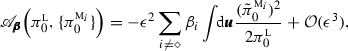 (82)
(82)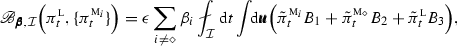 (83)
(83)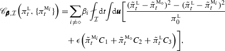 (84)
(84)where \(\{B_m\},\{C_m\},\,m=1,2,3\) are functions of \({\tilde{\pi }}^{{\textsc {m}}_i}_0,{\tilde{\pi }}^{{\textsc {m}}_{\diamond }}_0, {\tilde{\pi }}^{\textsc {l}}_0\) and \(\epsilon \). Note that unless \(\epsilon =0\) (so that \(\pi ^{{\textsc {m}}_i}_{0}=\pi _{0}^{\textsc {l}}\)), it is difficult to improve the prediction skill at short times within the MME framework since at \(t=0\), we have \({\fancyscript{B}}_{\pmb {\beta },{\mathcal {I}}}={\fancyscript{C}}_{\pmb {\beta },{\mathcal {I}}}=0\) and \({\fancyscript{A}}_{\pmb {\beta }}<0\) in (80).


Rights and permissions
About this article

Cite this article
Branicki, M., Majda, A.J. An Information-Theoretic Framework for Improving Imperfect Dynamical Predictions Via Multi-Model Ensemble Forecasts. J Nonlinear Sci 25, 489–538 (2015). https://doi.org/10.1007/s00332-015-9233-1
Received:
Accepted:
Published:
Issue Date:
DOI: https://doi.org/10.1007/s00332-015-9233-1