
Abstract
The proof of convergence of adaptive discretization-based algorithms for semi-infinite programs (SIPs) usually relies on compact host sets for the upper- and lower-level variables. This assumption is violated in some applications, and we show that indeed convergence problems can arise when discretization-based algorithms are applied to SIPs with unbounded variables. To mitigate these convergence problems, we first examine the underlying assumptions of adaptive discretization-based algorithms. We do this paradigmatically using the lower-bounding procedure of Mitsos [Optimization 60(10–11):1291–1308, 2011], which uses the algorithm proposed by Blankenship and Falk [J Optim Theory Appl 19(2):261–281, 1976]. It is noteworthy that the considered procedure and assumptions are essentially the same in the broad class of adaptive discretization-based algorithms. We give sharper, slightly relaxed, assumptions with which we achieve the same convergence guarantees. We show that the convergence guarantees also hold for certain SIPs with unbounded variables based on these sharpened assumptions. However, these sharpened assumptions may be difficult to prove a priori. For these cases, we propose additional, stricter, assumptions which might be easier to prove and which imply the sharpened assumptions. Using these additional assumptions, we present numerical case studies with unbounded variables. Finally, we review which applications are tractable with the proposed additional assumptions.
1 Introduction
Adaptive discretization-based algorithms are widely used for the solution of semi-infinite programs (SIPs), generalized semi-infinite programs, and bilevel programs, e.g., Hettich and Kortanek (1993), Winterfeld (2008), Mitsos and Barton (2007), López and Still (2007), Küfer et al (2008). For a recent review of applications and adaptive discretization-based algorithms for SIPs, the reader may refer to Djelassi et al (2021). In this paper, we consider SIPs in the form of

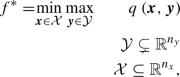
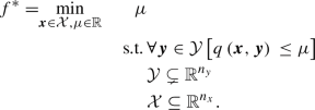
with the sets \(\mathcal {X}\subseteq {\mathbb {R}}^{n_{x}}\) and \(\mathcal {Y}\subseteq {\mathbb {R}}^{n_{y}}\) with \(\left|\mathcal {Y}\right|= \infty \); the constraint function \(g : \mathcal {X} \times \mathcal {Y} \rightarrow {\mathbb {R}}\); and the objective function \(f : \mathcal {X} \rightarrow {\mathbb {R}}\) with \(f^{*}\) being the optimal objective value. Note that the semi-infinite constraint  is often written in literature as
  .
.
Conceptually, adaptive discretization-based algorithms for (SIP) replace the infinite index set \(\mathcal {Y}\) with a finite one, i.e., \(\mathcal {Y}^{k} \subsetneq \mathcal {Y}\), with k being the iteration index. This, then finite program, is an approximation of (SIP). Using an adaptive refinement strategy for the finite index set \(\mathcal {Y}^{k} \subsetneq \mathcal {Y}^{k+1}... \subsetneq \mathcal {Y}\), one obtains an improving approximation of (SIP), which usually yields a converging lower bound. Hence, one obtains a lower-bounding procedure.
In this paper, we paradigmatically consider the lower-bounding procedure of Mitsos (2011). Mitsos applies a convergent lower-bounding procedure as well as proposes a convergent upper-bounding procedure to compute in finite time a feasible point of (SIP) with a certificate of \(\varepsilon ^{f}\)-optimality. The upper-bounding procedure of Mitsos is a slight adaption of the lower-bounding procedure. The lower-bounding procedure in turn is equivalent to the algorithm by Blankenship and Falk (1976) which can be considered as the main representative of adaptive discretization-based algorithms. Moreover, many adaptive discretization-based algorithms for (generalized) semi-infinte programs and bilevel programs have identical predecessors, i.e., the previously mentioned Blankenship and Falk (1976) which itself is based on Remez (1962). These algorithms are conceptually closely related to, e.g., Reemtsen (1991), Still (1999, 2001), Stein (2003), Mitsos et al (2008a), Guerra Vázquez et al (2008), Tsoukalas and Rustem (2011), Mitsos and Tsoukalas (2015), Djelassi and Mitsos (2017, 2021), Seidel and Küfer (2020), Djelassi et al (2019), Schwientek et al (2021). Therefore, and also based on our additional findings, c.f., Appendix B, we expect that the results within this paper, i.e., convergence guarantees with the sharper, slightly relaxed, assumptions and recovered convergence guarantees in case of unbounded variables, directly carry over from one algorithm to the other.
The proof of convergence of algorithms for the global solution of SIPs often relies, among other assumptions, on compact host sets. This is true both for discretization-based and other methods as well as local methods allowing nonconvex lower-level problems (Bhattacharjee et al 2005a, b; Floudas and Stein 2008; Mitsos et al 2008b). Another popular assumption within literature is the one of a compact lower-level set (Reemtsen and Görner 1998). This assumption is fulfilled if (SIP) is feasible, the host sets are compact, and the functions f and g are continuous. The advantage of this assumption is that it already allows special cases of SIPs with unbounded sets \(\mathcal {X}\). However, unbounded sets \(\mathcal {Y}\) are not covered. Typically, the upper- and lower-level variables \(\varvec{x}\) and \(\varvec{y}\) have a technical or physical meaning and thus, in most cases, inherit finite bounds from their physical or technical origin. Furthermore, these finite bounds are usually attainable yielding closed and therefore compact upper- and lower-level host sets \(\mathcal {X}\) and \(\mathcal {Y}\).
However, one might not know the finite bounds of the variables. Furthermore, SIPs stemming from specific applications or reformulations may exhibit unbounded upper- and/or lower-level variables, and hence unbounded upper- and/or lower-level host sets. In the following, we give examples of problem classes where SIPs with unbounded host sets can arise. Note that in some of the applications, finite bounds of the variables may be computed or generated by additional assumptions. In most of the following examples, (arbitrary) bounds are usually used in practice. An unbounded lower-level set \(\mathcal {Y}\) may occur, e.g., in approximation theory where one wants to approximate a function with a minimal estimation error, not only over a compact set, but over all \({\mathbb {R}}^{n}\) (Chebyshev approximation). An unbounded upper-level variable host set \(\mathcal {X}\) occurs, e.g., in design centering, in epigraph reformulations of min-max programs or in approximation theory, e.g., classical Chebyshev problem, where the parameter values are unbounded, or reverse Chebyshev approximation, where the approximation error is fixed and the region where the approximation is not worse than the fixed approximation error is computed (Still 1999; Guerra Vázquez et al 2008).
In order to address such applications, we will investigate whether adaptive discretization-based algorithms are directly applicable to SIPs with unbounded host sets, i.e., whether the assumption of compact host sets can be relaxed. By relaxing the assumption of compact host sets, we will also consider SIPs with bounded but noncompact host sets, e.g., host sets consisting of half-open intervals or open intervals. For cases where the assumptions are not directly applicable, we will derive additional assumptions, which are possibly easier to prove, to enable the application.
In Sect. 2, we first introduce the basic notation used throughout this paper and review the assumptions in Mitsos (2011). Second, we prove convergence of the lower-bounding procedure. In the proof, we use sharper and slightly relaxed assumptions compared to Mitsos (2011), which in turn are already relaxed compared to Blankenship and Falk (1976). We show that our relaxed assumptions are implied by the original assumptions of Mitsos (2011). Section 3 shows that the lower-bounding procedure may exhibit convergence problems if the host sets are not compact. In Sect. 4, we give additional assumptions to apply the lower-bounding procedure to SIPs with noncompact and unbounded host sets. In Sect. 5, we present two case studies as a proof-of-concept for our findings. Finally, we give a conclusion and outlook in Sect. 6.
2 Preliminaries
In this section, we briefly review the notation, formulation, definitions, algorithm description, and assumptions of the lower-bounding procedure in Mitsos (2011). Note that this procedure can be seen paradigmatically for the class of adaptive discretization-based algorithms.
2.1 Notation, formulation, definitions and algorithm description
The iterative lower-bounding procedure is illustrated in Fig. 1. At the start of the procedure the iteration index k is set \(k \leftarrow 0\) and a (arbitrary) finite set \(\mathcal {Y}^{0} \subsetneq \mathcal {Y}\) is chosen. Then the discrete lower-bounding problem (LBP) is solved.
Definition 1
(Discrete lower-bounding problem) The discrete lower-bounding problem (LBP) with \(\mathcal {Y}^{k} \subsetneq \mathcal {Y}\) is

In literature, (LBP) is also often called discrete upper-level problem.
Due to \(\mathcal {Y}^{k} \subsetneq \mathcal {Y}\), (LBP) is a relaxation of (SIP) and it holds  . For the optimal solutions of (LBP), we use the notation
Notation 1
(Optimal solution of (LBP)) Assuming the optimal solution of (LBP) exists in all iterations, we denote the optimal solution point by \(\varvec{x}^{k}\) and the sequence of optimal solutions by \(\left\{ \varvec{x}^{k}\right\} _{k=0}^{m} = \left\{ \varvec{x}^{0}, \varvec{x}^{1}, \varvec{x}^{2},..., \varvec{x}^{m}\right\} \). To simplify the notation, we omit indexing numbers wherever possible, i.e., \(\left\{ \varvec{x}^{k}\right\} \).
If (LBP) is determined unbounded, then by Assumption 4 (to follow), also (SIP) is unbounded. If (LBP) is determined infeasible, also (SIP) is infeasible. Otherwise, the lower-level problem (LLP) is solved to determine SIP-feasibility of the current iterate.
Definition 2
(Lower-level problem) The lower-level problem (LLP) for fixed upper-level variables \(\varvec{x}^{k}\) is

The iterate \(\varvec{x}^{k}\) is SIP-feasible if  . Note that according to the later used Assumption 3, (LLP) may only be solved approximately. For the optimal and approximate solution of (LLP), we use the notation
Notation 2
(Optimal solution of (LLP)) Assuming the optimal solution of (LLP) exists in all iterations, we denote the optimal solution point by \(\varvec{y}^{*,k}\) and the sequence of optimal solutions by \(\left\{ \varvec{y}^{*,k}\right\} _{k=0}^{m} = \left\{ \varvec{y}^{*,0}, \varvec{y}^{*,1}, \varvec{y}^{*,2},..., \varvec{y}^{*,m}\right\} \). To simplify the notation, we omit indexing numbers wherever possible, i.e., \(\left\{ \varvec{y}^{*,k}\right\} \).

Notation 3
(Approx. solution of (LLP)) Assuming the approximate solution of (LLP) exists in all iterations, we denote the approximate solution point by \(\varvec{y}^{k}\) and the sequence of approximate solutions by \(\left\{ \varvec{y}^{k}\right\} _{k=0}^{m} = \left\{ \varvec{y}^{0}, \varvec{y}^{1}, \varvec{y}^{2},..., \varvec{y}^{m}\right\} \). To simplify the notation, we omit indexing numbers wherever possible, i.e., \(\left\{ \varvec{y}^{k}\right\} \).
To ease notation, we also use Notation 1 to 3 for infinite sequences. Note that this is abuse of notation as in these cases no maximum iteration index m exists.
When (LLP) is solved approximately according to the later used Assumption 3, it is either determined that  or an approximate solution point \(\varvec{y}^{k}\) is furnished which fulfills
  for some \(\alpha \in \left( 0,1\right] \). As finite termination to a feasible point is not guaranteed, in practice a feasibility tolerance
  is usually introduced as a termination criterion. In this case, the algorithm may terminate with an SIP-\(\varepsilon ^{a}\)-feasible point which suffices
  . If \(\varvec{x}^{k}\) is not SIP-(\(\varepsilon ^{a}\))-feasible, the approximate solution of (LLP) is used to populate the discretization set \(\mathcal {Y}^{k}\) for subsequent iterations.
A feasibility tolerance  is used in the numerical case studies in Sect. 5. However, note that in the theoretical considerations, no feasibility tolerance is introduced, or equivalently the feasibility tolerance is set to zero, i.e., \(\varepsilon ^{a} = 0\). Therefore, in the following theoretical analysis, especially in the proof of convergence in Sect. 2.3, one does not terminate early, but considers the full (infinite) sequence of iterates.
The following is a summary of additional notation and the definition of compact sets used in this work.
Notation 4
(Feasible set) We use for the set of all feasible points in the host set of (SIP) the notation

Notation 5
(Infeasible set) We use for the set of all infeasible points in the host set of (SIP) the notation
Definition 3
(Compact set) \(\mathcal {K}\subsetneq {\mathbb {R}}^{n}\) is compact if any open cover of \(\mathcal {K}\) has a finite subcover. More explicitly, \(\mathcal {K}\) is compact if whenever \(\mathcal {K} \subseteq \bigcup _{\alpha \in \mathcal {I}} \mathcal {A}_{\alpha }\), where each \(\mathcal {A}_{\alpha }\) is open, there exists a finite number of indices \(\alpha _{1},\) \(\alpha _{2},\) \(..., \alpha _{m} \in \mathcal {I}\) such that \(\mathcal {K} \subseteq \bigcup _{j=1}^{j=m} \mathcal {A}_{\alpha _{j}}\) (c.f., Jänich 2008).
2.2 Assumptions
The existing global discretization-based algorithms use a global solver to compute the subproblems (LBP) and (LLP) which are (mixed-integer) (non)linear problems ((MI)(N)LP). By considering SIPs with unbounded host sets, we obviously inherit the need for global solvers that can handle optimization problems with unbounded host sets. In the case of linear programs, this does not pose a problem as, e.g., the simplex method can handle unbounded host sets (Nocedal and Wright 1999). In the more general case of (MI)NLPs, e.g., BARON is able to treat some problems with unbounded variables systematically by trying to compute appropriate bounds from problem constraints (Khajavirad and Sahinidis 2018) but substantial theoretical and practical challenges remain. In what follows, we focus on the SIP algorithm’s convergence properties for unbounded host sets and do not discuss these challenges.
The presented lower-bounding procedure in Mitsos (2011), which is equivalent to the procedure proposed by Blankenship and Falk (1976), relies on the following assumptions (c.f., Lemma 2.2 in Mitsos (2011), revised in Lemma 2 in Harwood et al (2021)):
Assumption 1
(Compactness of sets) The sets \(\mathcal {X} \subsetneq {\mathbb {R}}^{n_x} \) and \(\mathcal {Y} \subsetneq {\mathbb {R}}^{n_y}\) are compact.
Assumption 2
(Continuous functions) The functions f and g are continuous on \(\mathcal {X}\) and \(\mathcal {X} \times \mathcal {Y}\), respectively.
Assumption 3
(Appr. solution of (LLP)) At each iteration k, (LLP) is solved approximately for the solution of the lower-bounding problem \(\varvec{x}^{k}\) either establishing  , or furnishing a point \(\varvec{y}^{k}\) such that
  . With \(\alpha \) being constant over all iterations and \(\alpha \in \left( 0,1\right] \).
Assumption 3 is relaxed compared to the assumption in Blankenship and Falk (1976), where the exact solution of (LLP) is assumed. It is also slightly relaxed to Harwood et al (2021) wherein \(\alpha \) is restricted to
\(\left( 0,1\right) \). However, as will be shown below, the problems associated with unbounded host sets persist even if the (LLP) is solved exactly.
2.3 Proof of convergence of the lower-bounding procedure
The proof presented in this paper relies on slightly relaxed assumptions compared to those made by Mitsos (2011) and Reemtsen and Görner (1998). Basically, we split the assumptions made by Mitsos (2011) and some properties, which result from them, into multiple sharpened assumptions. Additionally, we use the idea of level sets by Reemtsen and Görner (1998). These sharpened assumptions are often challenging to prove a priori. In these cases, we later present alternative, stricter, assumptions, which are easier to prove and that imply the sharpened assumptions. The sharpened assumptions motivate the additional, stricter, assumptions, which might be easier to prove, for SIPs with unbounded host sets in Sect. 4.
Section 1 is relaxed to
Assumption 4
It holds (a)  and (b) \(\Lambda \left( \mathcal {Y}^{0}\right) \) is bounded with the set \(\Lambda \left( \mathcal {Y}^{0}\right) \) defined as

whereas \(f^{*}\) is the optimal objective value of (SIP).
Remark 1
Assumption 4 builds on the consideration that the algorithm must only exclude points which
-
are super-optimal, i.e., points which belong to the lower level-set
 ,
, -
are feasible within the initially chosen discretization \(\mathcal {Y}^{0}\), and
-
belong to \(\mathcal {X}^{\mathrm {infeas}}\).
 ,
,If the iterate is not an element of \(\Lambda \left( \mathcal {Y}^{0}\right) \), the iterate is feasible and optimal by assumption. Note that if (SIP) is infeasible we have by convention \(f^{*}=+\infty \) and therefore  .
.
Assumption 4 allows for unbounded host sets and also for bounded but not closed sets. In Sect. 4 we give examples of stronger assumptions or checks which can be performed since the assumption is difficult to verify a priori. The property of uniform continuity of f and g on \(\mathcal {X}\) and \(\mathcal {X}\times \mathcal {Y}\), respectively, follow from Assumptions 1 and 2. In the following we relax these two assumptions.
Assumption 5
The function f is lower semi-continuous at all \(\varvec{x} \in \partial \Lambda \left( \mathcal {Y}^{0}\right) \).
Assumption 6
It holds

We first prove that the proposed assumptions are indeed relaxed compared to the original assumptions, i.e., the latter imply the former.
Lemma 1
Assumptions 4 to 6 hold if Assumptions 1 and 2 are satisfied.
Proof
First, we show that Assumption 1 implies Assumption 4. \(\mathcal {X}\) is compact according to Assumption 1. Since \(\Lambda \left( \mathcal {Y}^{0}\right) \subseteq \mathcal {X}\), we directly get  . \(\mathcal {X}\) is bounded by compactness and, therefore, \(\Lambda \left( \mathcal {Y}^{0}\right) \) is also bounded.
Second, according to Assumption 2, f is continuous on \(\mathcal {X}\) and hence lower semi-continuous on \(\partial \Lambda \left( \mathcal {Y}^{0}\right) \subseteq \mathcal {X}\), or Assumption 5 holds.
Third, from Assumptions 1 and 2 follows uniform continuity of g on \(\mathcal {X}\times \mathcal {Y}\) and we have

Then, it also holds

because \(\left\{ \varvec{x}^{k}\right\} \cap \Lambda \left( \mathcal {Y}^{0}\right) \subseteq \mathcal {X}\) and \(\Lambda \left( \mathcal {Y}^{0}\right) \subseteq \mathcal {X}\). \(\square \)
Next, we prove convergence of the lower-bounding procedure using Assumption 3 and the relaxed Assumptions 4 to 6. Recall, that no feasibility tolerance \(\varepsilon ^{a}\) is introduced and, hence, the full (infinite) sequence of iterates is considered.
Theorem 1
If Assumptions 3 to 6 are satisfied, the adaptive discretization-based lower-bounding procedure in Mitsos (2011) terminates finitely with the optimal objective value or converges to the optimal objective value, i.e., \(f^{k} \rightarrow f^{*}\) for \(k \rightarrow \infty \). If the SIP is infeasible or unbounded, the lower-bounding procedure terminates finitely with proof of infeasibility or unboundedness, respectively.
Note that Reemtsen and Görner (1998) and Mitsos (2011) exclude infeasible SIPs by assumption, c.f., Assumption 12 in Appendix B.
Proof
We first show that we move away from any compact set of infeasible points within finitely many iterations. Second, we consider the case of an infeasible SIP. We show that the algorithm terminates finitely with proof of infeasibility. Third, we consider the case of a feasible SIP and show that the algorithm terminates finitely with a globally optimal solution, or the algorithm produces the optimal solution in the limit.
-
1.
Consider a compact set of infeasible points \(\mathcal {K}^{\text {infeas}} \subseteq \Lambda \left( \mathcal {Y}^{0}\right) \). In the following, we restrict the iterations to be in this set, i.e., \(\varvec{x}^{k} \in \left\{ \varvec{x}^{k}\right\} \cap \mathcal {K}^{\text {infeas}}\). Recall that
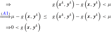
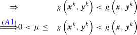
 would imply that \(\varvec{x}^{k}\) is feasible, \(\varvec{x}^{k}\) is not a member of \(\mathcal {K}^{\text {infeas}}\), and we have left \(\mathcal {K}^{\text {infeas}}\). Due to Assumption 3, we have
  (7)
(7)Since Assumption 6 holds for all
 , it also holds
 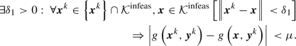 (8)
(8)We obtain for the deduction in (8) the two cases for \(\varvec{x}\in \mathcal {K}^{\mathrm {infeas}}\)
-
Case 1:
 :
: 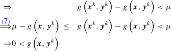 (9)
(9) -
Case 2: \(g\left( \varvec{x}^{k},\varvec{y}^{k}\right) - g\left( \varvec{x},\varvec{y}^{k}\right) {}<0\):
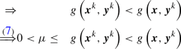 (10)
(10)
Therefore, it holds
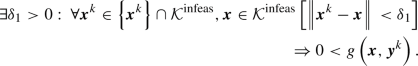 (11)
(11)Thus, with each iteration, the open neighborhood \(\mathcal {N}_{\delta _{1}}\left( \varvec{x}^{k}\right) \cap \mathcal {K}^{\text {infeas}}\) is infeasible for the following iterations (and therefore we do not (re)visit points in this neighborhood). Since the excluded neighborhoods cannot be revisited and \(\mathcal {K}^{\text {infeas}}\) is compact, after at most finitely many iterations, these neighborhoods form a finite cover of \(\mathcal {K}^{\text {infeas}}\). Therefore, we only need a finite number of iterations until we have covered \(\mathcal {K}^{\text {infeas}}\) (c.f., Definition 3), i.e., we prove infeasibility of all points in \(\mathcal {K}^{\text {infeas}}\) after a finite number of iterations.
-
-
2.
Consider now an infeasible SIP. \(\Lambda \left( \mathcal {Y}^{0}\right) \) is compact by Assumption 4. The proof of finite termination with proof of infeasibility directly follows from the proof for case 1 above with \(\mathcal {K}^{\text {infeas}} = \Lambda \left( \mathcal {Y}^{0}\right) \). It follows that (LBP) is infeasible after a finite number of iterations.
-
3.
Finally, consider a feasible SIP.
-
(a)
If (SIP) is unbounded, the problem will be determined to be unbounded in the first iteration. (LBP) is a valid relaxation of (SIP), i.e.,
 . As (SIP) is by assumption unbounded, also (LBP) is in the first iteration unbounded, i.e.,
  . By Assumption 4,
  and the unbounded solution is feasible.
 -
(b)
If the optimal solution is finite, i.e.,
 , we will show by contradiction that a feasible and optimal point is generated in the limit.
By Assumption 4, there exists a compact set \(\widetilde{\mathcal {X}} \supsetneq \Lambda \left( \mathcal {Y}^{0}\right) \) containing the optimal point. By compactness of \(\widetilde{\mathcal {X}}\), we can choose an infinite subsequence \(\left\{ \varvec{x}^k\right\} \) that converges to \(\hat{\varvec{x}} \in \widetilde{\mathcal {X}}\).
Now, assume the limit point is infeasible \(\hat{\varvec{x}} \in \mathcal {X}^{\text {infeas}}\). There exists a compact set \(\mathcal {K}^{\text {infeas}} \ni \hat{\varvec{x}}\). By proof from case 1 above, we move away from any infeasible set \(\mathcal {K}^{\text {infeas}}\) within finite time. Therefore, the infeasible point \(\hat{\varvec{x}}\) is not a limit point that gives us the desired contradiction.
It remains to show that the feasible limit point is optimal. (LBP) is a valid relaxation of (SIP). Hence, we have
 . The limit point \(\hat{\varvec{x}}\) is feasible, i.e.,
  and in the boundary of \(\Lambda \left( \mathcal {Y}^{0}\right) \). With lower semi-continuous of f at all \(\forall \varvec{x} \in \partial \Lambda \left( \mathcal {Y}^{0}\right) \) and with
  follows \(f\left( \hat{\varvec{x}}\right) = f^{*}\). \(\square \)
-
(a)
 would imply that
 , it also holds
 :
: 


 . As (SIP) is by assumption unbounded, also (LBP) is in the first iteration unbounded, i.e.,
  . By Assumption
  and the unbounded solution is feasible.
 , we will show by contradiction that a feasible and optimal point is generated in the limit.
 . The limit point
  and in the boundary of
  follows
 Following the proof of Lemma 1 and Theorem 1, we can also prove that the lower-bounding procedure in Mitsos (2011) converges in the infeasible case under the original Assumptions 1 to 3. The proof is also applicable with slight changes for a lower-semicontinuous constraint function g on \(\mathcal {X}\) for all \(\varvec{y} \in \mathcal {Y}\). This property might be of interest in cases where the constraint function resembles the solution of an embedded optimization problem. The reader may refer to Appendix A.1 for the corresponding proposition and proof.
The upper-bounding procedure in Mitsos (2011) is conceptually similar to the lower-bounding procedure. The proof of convergence and the slightly changed assumptions for the case of unbounded host sets of the upper-bounding procedure are shown in Appendix B.3. This particular supports our claim that the results of our work can be directly transferred to other conceptually similar procedures.
3 Illustrative examples of SIPs with unbounded host sets
We first show examples where Assumptions 3 to 6 do not hold and discuss how the lower-bounding procedure may fail. All examples follow the same pattern. They contain an upper- or lower-level variable that i) has an unbounded host set and ii) can be chosen arbitrarily in the sense that the variable does not affect the (LBP) or (LLP) objective, respectively. Using this property, we can choose a sequence of points that generates arbitrarily weak discretization cuts, thus violating Assumption 6. This leads to a convergence to an infeasible point in the limit with no proof of infeasibility
3.1 Illustrative example for \(\mathcal {X}\) compact and \(\mathcal {Y}\) unbounded
Consider the SIP

Note that the corresponding LLP has infinitely many solutions. The optimal solutions of (LLP) are \(\varvec{y}^{*}\left( {\bar{x}}\right) = \left( {\tilde{y}}, {\bar{x}}\right) ^{T}\) or \(\varvec{y}^{*}\left( {\bar{x}}\right) = \left( 0,{\tilde{y}}\right) ^{T}\) with arbitrary \({\tilde{y}} \in {\mathbb {R}}\). We have  . Therefore, (E1) is infeasible.
Now, we show that the lower-bounding procedure may converge to an infeasible point. We start with an empty discretization \(\mathcal {Y}^{0} = \emptyset \). The optimal solution of the (LBP) is \(x^{0}=2\) with an optimal objective value of \(f^{0}=-2\). Then, \(\varvec{y}^{*,0}=\left( 2, 2\right) ^{T}\) is a globally optimal solution of (LLP). Using \(\varvec{y}^{*,k}=\left( 2^{k+1}, x^{k}\right) ^{T}\) for all subsequent iterations and considering the (LBP) objective, the last introduced discretization point determines the optimal solution in the next iteration. See also Fig. 2 for graphical illustration. \(x^{k+1}\) can be computed by

Therefore, we have for any iteration 

Illustrative example (E1) for \(\mathcal {X}\) compact and \(\mathcal {Y}\) unbounded with parametric solutions of (LLP). (E1) is infeasible.
With \(\sum _{i=1}^{k} \frac{1}{2^i}\) being the geometrical series, we obtain \(\lim _{k\rightarrow \infty } x^0 -\sum _{i=1}^{k} \frac{1}{2^i} = 1\) with an objective value of \(f^{k=\infty }=-1\). Therefore, the lower-bounding procedure converges to an infeasible point in the limit, and no proof of infeasibility is given within finite time.
The same convergence issues arise when we consider an SIP with \(\mathcal {X}\) compact and \(\mathcal {Y}\) bounded but not closed, c.f., Appendix A.2.1. For the sake of simplicity, we considered the infeasible SIP (E1). Recall that Mitsos (2011), Reemtsen and Görner (1998) exclude infeasible SIPs. Therefore, (E1) would not be considered (assuming the extension to unbounded host sets). The reader may refer to the Appendix A.2.2 for a feasible but conceptually equivalent SIP that exhibits the same convergence issues.
We show in (E1) that in certain cases the lower-bounding procedure can converge to an infeasible point. Similarly, also, the upper-bounding procedure in Mitsos (2011) may never produce a SIP-feasible point, supporting our claim that our results carry over to other related adaptive discretization-based procedures. For a detailed example, the reader may refer to Appendix B.2.
3.2 Illustrative example for \(\mathcal {X}\) unbounded and \(\mathcal {Y}\) compact
Consider the SIP

The optimal value function of the corresponding (LLP) is  with the optimal solution \(y^{*}\left( \bar{\varvec{x}}\right) = {\bar{x}}_{2}\). Therefore, (E3) is infeasible. Note that the objective function only depends on \(x_{2}\) and is constant in the interval \(x_{2} \in \left[ 1,2\right] \). Again, we show below that the lower-bounding procedure can converge to an infeasible point in the limit. First, start with an empty discretization set \(\mathcal {Y}^{0} = \emptyset \). For iteration \(k=0\), choose \(\varvec{x}^{0}=\left( 4, 2\right) ^{T}\) as the optimal solution, with an objective value of \(f^{0}=-1\). For the corresponding (LLP), we have \(y^{*,0} = 2\). Using for iteration \(k\ge 1\) and all following iterations \(x_{1}^{k} = 2^{k+2}\) and considering the (LBP) objective, we can choose \(x_{2}^{k} = 2 - \sum _{i=1}^{k} \frac{1}{2^{i}}\), see Fig. 3 for graphical illustration.

Illustrative example (E3) for \(\mathcal {X}\) unbounded and \(\mathcal {Y}\) compact with parametric solutions of LLP. (E3) is infeasible.
With \(\sum _{i=1}^{k} \frac{1}{2^i}\) being the geometrical series, we obtain \(\lim _{k\rightarrow \infty } x_{2} = \lim _{k\rightarrow \infty } x_{2}^0 -\sum _{i=1}^{k} \frac{1}{2^i} = 1\) with an objective value of \(f^*=-1\). Therefore, the lower-bounding procedure does not prove infeasibility of (E3) within finite time.
Again, for the sake of simplicity, an infeasible SIP with a non-differentiable function f has been considered. Similar adaptations as in Appendix A.2.2 can be made to obtain a feasible SIP with n-times differentiable functions, which exhibit the same convergence issues. Furthermore, similar adaptions as in Appendix A.2.1 can be made to obtain an SIP with compact \(\mathcal {Y}\) and bounded but non-compact \(\mathcal {X}\), which exhibits the same convergence issues.
4 Examples of assumptions that are easier to prove than assumptions 4 to 6
As already shown in Sect. 2, the often encountered assumptions in literature for SIPs imply our slightly relaxed assumptions. However, for SIPs with unbounded host sets the former assumptions do not hold. In these cases, it is often not obvious whether the relaxed Assumptions 4 to 6 hold. This section, discusses additional (stricter) assumptions and criteria for different cases of SIPs with unbounded host sets which can be often checked a priori or during run-time to enable application.
4.1 Case 1: \(\mathcal {X}\) unbounded \(\mathcal {Y}\) compact
First, note that if the lower-bounding procedure produces a point outside \(\Lambda \left( \mathcal {Y}^{0}\right) \), the algorithm terminates (Remark 1). Hence, we restrict our discussion to the following cases:
-
1.1
\(\Lambda \left( \mathcal {Y}^{0}\right) \) is unbounded
-
1.2
\(\Lambda \left( \mathcal {Y}^{0}\right) \) is bounded
Feasible SIPs can belong to cases 1.1 or 1.2. Infeasible SIPs usually belong to case 1.1 if the initial discretization does not directly lead to an infeasible (LBP). If this is not the case, it follows from \(\mathcal {X}\) unbounded and \(\mathcal {X}^{\text {feas}} = \emptyset \) that \(\Lambda \left( \mathcal {Y}^{0}\right) \) is unbounded.
In the general case 1.1, the existence of a finite cover of the set \(\Lambda \left( \mathcal {Y}^{0}\right) \) cannot be guaranteed. Even if we exclude an open neighborhood of points whose size tends to infinity in each iteration, we cannot guarantee convergence. A different perspective offer Reemtsen and Görner (1998) who note that due to unboundness the proof of convergence fails as no limit point of \(\left\{ \varvec{x}^{k}\right\} \) may exist.
As a counterexample, revisit (E3) and replace g with the piecewise-defined function

In this case, the open ball we exclude in each iteration is infinite. However, the same convergence issues arise when using the same sequence of (LLP) solutions given in (E3).
The function g in Eq. 12 is continuous but not differentiable on \(\mathcal {X}\times \mathcal {Y}\). Similar to Remark 2, we can obtain a function belonging to differentiability class \(C^{n}\) that produces the same convergence issues.
Therefore, we concentrate in the following on case 1.2, i.e., \(\Lambda \left( \mathcal {Y}^{0}\right) \) is bounded. We will discuss stricter assumptions or checks which can often be applied to verify that case 1.2 holds irrespectively of \(\mathcal {X}\) unbounded. In detail, we will discuss
-
1.2.1
\(\mathcal {X}^{\text {feas}} \ne \emptyset \) and f is continuous and coercive on \(\mathcal {X}\), i.e.,
 .
. -
1.2.2
the (SIP) stems from the min-max program
 (13)
(13)with \(q : \mathcal {X} \times \mathcal {Y} \rightarrow {\mathbb {R}}\) and q being coercive in \(\varvec{x}\) for all \(\varvec{y}\). In this case, we consider in the following the epigraph reformulation of this min-max program, which reads
 (14)
(14) -
1.2.3
additional computational checks
 .
.

4.1.1 Case 1.2.1: f is continuous and coercive on \(\mathcal {X}\) and \(\mathcal {X}^{\text {feas}} \ne \emptyset \)
If f is continuous and coercive on \(\mathcal {X}\) and \(\mathcal {X}^{\text {feas}} \ne \emptyset \), we can prove convergence of the lower-bounding procedure.
Assumption 7
The set \(\mathcal {Y}\subsetneq {\mathbb {R}}^{n_y}\) is compact and  . f is continuous and coercive on \(\mathcal {X}\) and \(\mathcal {X}^{\text {feas}} \ne \emptyset \)
Proposition 1
Under Assumptions 2, 3 and 7, the lower-bounding procedure converges.
Proof
Because f is coercive on \(\mathcal {X}\) and \(\mathcal {X}^{\text {feas}} \ne \emptyset \), we have \(f^{*} < + \infty \) and the set  is bounded. Hence, also \(\Lambda \left( \mathcal {Y}^{0}\right) \) is bounded irrespective of \(\mathcal {Y}^{0}\). From boundness of \(\Lambda \left( \mathcal {Y}^{0}\right) \) and Assumption 7 follows
  . First, Assumption 4 is therefore satisfied. Second, from Assumption 7 follows Assumption 5. Third, from continuity of g (Assumption 2) and
  and compactness of \(\mathcal {Y}\) follow uniform continuity of g and Assumption 6 is satisfied. By Theorem 1, the lower-bounding procedure converges. \(\square \)
4.1.2 Case 1.2.2: SIP has the form of a epigraph reformulation
In the special case that (SIP) is the epigraph reformulation of a min-max problem with a coercive objective function, we can show that Assumption 4 holds irrespectively of unboundness of \(\mathcal {X}\).
Assumption 8
(SIP) has the form of (14), q is continuous and coercive in \(\varvec{x}\) for all \(\varvec{y}\), and \(\mathcal {Y}\) is compact.
Proposition 2
Under Assumptions 3 and 8, the lower-bounding procedure converges.
Proof
From continuity and coerciveness of q in \(\varvec{x} \ \forall \varvec{y}\) follows the optimal point exists, is finite, and attainable. It also follows, \(\exists M\) such that  . Because of the epigraph form of (14), the construction of (LBP), and the global solution of the subproblems, we also have
  . Combining these results above, there exists a compact \(\mathcal {K}\) such that \(\left\{ \varvec{x}^{k}\right\} \subseteq \mathcal {K} \subsetneq \mathcal {X}\) and \(\varvec{x}^{*} \in \mathcal {K}\).
Using \(\mathcal {K}\) instead of \(\mathcal {X}\) in (14), we obtain a new SIP, called \(\widetilde{\text {SIP}}\). From compactness of \(\mathcal {K}\) follows Assumptions 4 is satisfied. From Assumptions 8 follows Assumptions 5. From continuity of q and compactness of \(\mathcal {K}\) and \(\mathcal {Y}\) follows Assumptions 6. By Assumptions 1, the lower-bounding procedure converges.
It remains to show that the solution of \(\widetilde{\text {SIP}}\) and of the original SIP are equivalent. \(\widetilde{\text {SIP}}\) is a restriction of (14) because \(\mathcal {K} \subsetneq \mathcal {X}\). Since the optimal point of (14) is also feasible in \(\widetilde{\text {SIP}}\), the optimal solutions are equivalent. \(\square \)
4.1.3 Case 1.2.3: Additional computational checks
In some instances, one can show (analytically) that Assumptions 4 is satisfied by proving that 
 \(g\left( \varvec{x},\varvec{y}\right) \)
  holds for any sequence \(\left\{ \varvec{x}^{k}\right\} \) with
  for \(k \rightarrow \infty \). This can also be done in some cases computationally by solving the two problems (15) and (16) a priori. The computational burden is in most cases tractable because the problems are adaptions of (LLP). However, one must assume that g is continuous on
  .
.

If \(x^{\text {infeas},\text {UBD}}\) is bounded, \(\Lambda \left( \mathcal {Y}^{0}\right) \) is also bounded (Assumption 4(b)). We now verify if Assumption 4(a) holds. If the optimal objective value of

is greater than zero, there exist no points that belong to  but not to \(\mathcal {X}\). Because
  , Assumption 4(a) holds.
4.2 Case 2: \(\mathcal {X}\) compact and \(\mathcal {Y}\) unbounded
If one of the following assumptions holds instead of Assumption 1, no convergence issues occur.
Assumption 9
The set \(\mathcal {X}\subsetneq {\mathbb {R}}^{n_{x}}\) is compact and  holds
holds  .
.
Assumption 10
The optimal solution \(\varvec{y}^{k}\) of (LLP) exists for all iterates \(\varvec{x}^k\), and the sequence \(\left\{ \varvec{y}^{k}\right\} \) does not diverge, i.e.,  .
.
As shown before, Assumption 5 is satisfied if f is continuous on \(\mathcal {X}\). Furthermore, Assumption 9 holds if g is uniformly continuous on \(\mathcal {X} \times \mathcal {Y}\) and \(\mathcal {X}\) is compact.
Proposition 3
Under Assumptions 3, 5 and 9, the lower-bounding procedure converges.
Proof
First, from Assumption 9 follows Assumption 4. Second, Assumption 5 is fulfilled by proposition 3. Third, Assumption 6 is fulfilled by Assumption 9. By Theorem 1, the lower-bounding procedure converges. \(\square \)
Proposition 4
Under Assumptions 2, 3 and 10, the lower-bounding procedure converges.
Proof
Consider

with \(\widetilde{\mathcal {X}} = \mathcal {X}\) and the compact interval \(\widetilde{\mathcal {Y}} \subseteq \mathcal {Y}\) such that \(\left\{ \varvec{y}^{k}\right\} \in \widetilde{\mathcal {Y}}\). With Assumption 2 follows uniform continuity of g on \(\widetilde{\mathcal {Y}} \times \widetilde{\mathcal {X}}\). (\(\widetilde{\text {SIP}}\)) fulfills Assumptions 1 to 3. Therefore, Theorem 1 and its proof are applicable.
We will show by contradiction that the optimal objective value of the limit point of (\(\widetilde{\text {SIP}}\)) and the original SIP are equivalent, i.e., \(f\left( \tilde{\varvec{x}}^{*}\right) = f\left( \varvec{x}^{*}\right) \).
First, assume  . Since the functions g and f are the same for (\(\widetilde{\text {SIP}}\)) and the original SIP, we have
  , i.e., \(\tilde{\varvec{x}}^{*}\) is infeasible in the original SIP. Assumption 10 and
  prove \(\tilde{\varvec{x}}^{*}\) infeasible which gives us the desired contradiction. Second, assume
  which gives us (due to the same functions g and f) \(\widetilde{\mathcal {X}}^{\text {feas}} \subsetneq \mathcal {X}^{\text {feas}}\). But from \(\widetilde{\mathcal {Y}} \subseteq \mathcal {Y}\), follows \(\widetilde{\mathcal {X}}^{\text {feas}} \supseteq \mathcal {X}^{\text {feas}}\) which gives us the desired contradiction. From \(f\left( \tilde{\varvec{x}}^{*}\right) \nless f\left( \varvec{x}^{*}\right) \) and \(f\left( \tilde{\varvec{x}}^{*}\right) \ngtr f\left( \varvec{x}^{*}\right) \) follows \(f\left( \tilde{\varvec{x}}^{*}\right) = f\left( \varvec{x}^{*}\right) \). \(\square \)
Assumption 10 generally cannot be proven a priori. Therefore, it is not directly applicable. However, stronger conditions than required for Assumption 10 can be checked a priori. For example, one may choose some large number M a priori and check during runtime whether  holds. One way to achieve this may be to require the solver to minimize the magnitude of the variable values among all global solutions of (LLP). The auxiliary problem

is solved with \({\bar{y}}\) being the optimal solution of the (LLP). Note that only an approximate solution of the (LLP) is required, c.f., Assumption 3. Therefore, a relaxation of the equality constraint is possible. The optimal solution of (AUX) is then used to populate the set \(\mathcal {Y}^{k}\).
We must point out that if one chooses a too large M in combination with a too restrictive maximum number iteration, the test may be inconclusive. Furthermore, populating the set \(\mathcal {Y}^{k}\) with the solution of (AUX) may be counterproductive in certain cases. One could also prove that Assumption 10 holds, by computing upper and lower bounds for each lower-level variable \(y_{i}\) a priori. The following optimization-based bound tightening based approach computes upper and lower bounds for all \(y_{i}\), i.e., \(y_{i}^{\text {UBD}}\) and \(y_{i}^{\text {LBD}}\), respectively. However, there is no guarantee of success.


Note the direction of the inequality in (17) and (18) as we want to compute the maximum and minimum value of \(y_{i}\) on  .
.
4.3 Case 3: \(\mathcal {X}\) unbounded and \(\mathcal {Y}\) unbounded
For SIPs with unconstrained upper- and lower-level hosts, convergence can be guaranteed if a suitable combination of the assumptions presented in Sect. 4.2 and Sect. 4.1 are adopted. Note that this is possible, as none of the corresponding pairs are mutually exclusive.
5 Numerical case studies
We present two illustrative case studies from Chebyshev approximation. These are a proof-of-concept for our findings rather than a complete numerical study which is beyond the scope of this paper. The corresponding (LBP) and (LLP) of the considered cases studies are written in the domain specific language libALE (Djelassi and Mitsos 2020). The implementation of the lower-bounding procedure is provided by the library for discretization-based semi-infinite programming solvers (libDIPS) (Djelassi 2020). The termination tolerance of the lower-bounding procedure is set to \(\varepsilon ^{a}=10^{-3}\). The default values for BARON are used with the exception of the optimality tolerances EpsA and EpsR which are set to \(10^{-9}\). The numerical case studies are carried out on a Windows Server 2016 Standard with an Intel(R) Xeon(R) CPU E5-2640 v3 @2.60GHz processor and 128GB of RAM. All subproblems are solved using BARON version 19.12.7., accessed through GAMS version 30.2.0 (Khajavirad and Sahinidis 2018; GAMS Development Corporation 2019). Note that BARON cannot handle trigonometric functions, which limits the applicability, and does not give certificate of global optimality for complex subproblems.
5.1 Case study for \(\mathcal {X}\) unbounded and \(\mathcal {Y}\) compact
Consider the min-max problem inspired by Chebyshev-approximation

with the auxiliary functions p and h defined as
We reformulate (19) to

Note that we have in this example the case of Sect. 4.1.2, i.e., the SIP has the form of an epigraph reformulation. The lower-bounding procedure terminates after 11 iterations (total CPU time \(19.5\hbox {s}\)) with an optimal solution of \(\varvec{x}^{*} = \left( -2.111, 6.471, -4.377, 1.091, -0.088\right) ^{T} \) and with a maximal error of the fit of 0.028 (Fig. 4).

Case study for \(\mathcal {X}\) unbounded and \(\mathcal {Y}\) compact. The original function is plotted as a green dashed line and the approximation function as a red solid line
5.2 Case study for \(\mathcal {X}\) compact and \(\mathcal {Y}\) unbounded
Consider

(21) corresponds to a reformulated min-max Chebyshev-approximation problem, where \(\left( \frac{3}{y^{2}} - \frac{2}{y^{3}} \right) \) is approximated by \(\exp \left( {x_{1} \left( x_{2} y + x_{3}\right) ^{2}}\right) \) over \(\left[ 1,+\infty \right) \) with \(\varvec{x}\) being the parameters to be estimated. For (21), Assumption 10 holds. The lower-bounding procedure terminates after 8 iterations (total CPU time 23.3s) with the optimal parameters \(\varvec{x}^{*} = \left( -0.010,-4.285, 1.248\right) ^{T}\) (Fig. 5).

Case study for \(\mathcal {X}\) compact and \(\mathcal {Y}\) unbounded. The original function is plotted as a green dashed line and the approximation function as a red solid line
6 Conclusion and outlook
Unconstrained upper and/or lower variable host sets in SIPs may arise, e.g., in (inverse) Chebyshev approximation, epigraphic reformulations, or design centering. In this paper, we showed that adaptive discretization-based algorithms are not suitable for all SIPs with unbounded host sets since convergence problems may arise.
Therefore, we investigated under which circumstances adaptive discretization-based algorithms are applicable to SIPs with unbounded host sets. The study was carried out using the lower-bounding procedure of Mitsos (2011) which can be considered representative of the class, since the procedure is equivalent to the one proposed by Blankenship and Falk (1976). First, we briefly reviewed the assumptions of the lower-bounding procedure. Instead of the original assumptions, we used sharper, (slightly) relaxed, assumptions for our proof of the convergence of the lower-bounding procedure. In essence, the sharpened, slightly relaxed, assumptions establish a weaker form of uniform continuity of the constraint function on the set of all infeasible points in the host set of the SIP. In addition, the objective function must be at least semi-continuous on the boundary of a subset of the infeasible points.
For SIPs with unbounded host sets, it is often not obvious whether the relaxed assumptions hold. We discusse additional (stricter) assumptions and criteria for different cases of SIPs with unbounded host sets which can be often checked a priori or during run-time to enable application. The criteria are expected to be, at most, of the same computational burden as the subproblems of the SIPs. The additional assumptions and criteria are expected to apply to many applications. Finally, we give two numerical case studies of SIPs with unbounded host sets, as a proof of concept.
Moreover, we assume that our results are transferable to conceptually related adaptive discretization-based procedures for generalized semi-infinite programs and bilevel programs, e.g., the algorithms proposed by Mitsos and Tsoukalas (2015); Djelassi et al (2019). We show that this assumption is justified by also considering the conceptually related upper-bounding procedure of Mitsos (2011) (Appendix B). However, for future work, we plan to investigate this for the named procedures in detail.
References
Bhattacharjee B, Green WH, Barton PI (2005a) Interval methods for semi-infinite programs. Comput Optim Appl 30(1):63–93. https://doi.org/10.1007/s10589-005-4556-8
Bhattacharjee B, Lemonidis P, Green WH Jr et al (2005b) Global solution of semi-infinite programs. Math Program 103(2):283–307. https://doi.org/10.1007/s10107-005-0583-6
Blankenship JW, Falk JE (1976) Infinitely constrained optimization problems. J Optim Theory Appl 19(2):261–281. https://doi.org/10.1007/BF00934096
Djelassi H (2020) Discretization-based algorithms for the global solution of hierarchical programs. Dissertation, RWTH Aachen University, Aachen. https://doi.org/10.18154/RWTH-2020-09163
Djelassi H, Mitsos A (2017) A hybrid discretization algorithm with guaranteed feasibility for the global solution of semi-infinite programs. J Glob Optim 68(2):227–253. https://doi.org/10.1007/s10898-016-0476-7
Djelassi H, Mitsos A (2020) libale—a library for algebraic logical expression trees. https://git.rwth-aachen.de/avt.svt/public/libale
Djelassi H, Mitsos A (2021) Global solution of semi-infinite programs with existence constraints. J Optim Theory Appl 188(3):863–881. https://doi.org/10.1007/s10957-021-01813-2
Djelassi H, Glass M, Mitsos A (2019) Discretization-based algorithms for generalized semi-infinite and bilevel programs with coupling equality constraints. J Glob Optim 92(3):453. https://doi.org/10.1007/s10898-019-00764-3
Djelassi H, Mitsos A, Stein O (2021) Recent advances in nonconvex semi-infinite programming: applications and algorithms. EURO J Comput Optim 9(5):100006. https://doi.org/10.1016/j.ejco.2021.100006
Falk JE, Hoffman K (1977) A nonconvex max–min problem. Nav Res Logist Q 24(3):441–450. https://doi.org/10.1002/nav.3800240307
Floudas CA, Stein O (2008) The adaptive convexification algorithm: a feasible point method for semi-infinite programming. SIAM J Optim 18(4):1187–1208. https://doi.org/10.1137/060657741
GAMS Development Corporation (2019) General algebraic modeling system (GAMS). http://www.gams.com/
Guerra Vázquez F, Rückmann JJ, Stein O et al (2008) Generalized semi-infinite programming: a tutorial. J Comput Appl Math 217(2):394–419. https://doi.org/10.1016/j.cam.2007.02.012
Harwood SM, Papageorgiou DJ, Trespalacios F (2021) A note on semi-infinite program bounding methods. Optim Lett 15(4):1485–1490. https://doi.org/10.1007/s11590-020-01638-4
Hettich R, Kortanek KO (1993) Semi-infinite programming: theory, methods, and applications. SIAM Rev 35(3):380–429. https://doi.org/10.1137/1035089
Jänich K (2008) Topologie, 8th edn. Springer-Lehrbuch, Springer, Berlin, https://doi.org/10.1007/978-3-540-26828-4
Khajavirad A, Sahinidis NV (2018) A hybrid LP/NLP paradigm for global optimization relaxations. Math Program Comput 10(3):383–421. https://doi.org/10.1007/s12532-018-0138-5
Küfer KH, Stein O, Winterfeld A (2008) Semi-infinite optimization meets industry: a deterministic approach to gemstone cutting. SIAM News 41(8):66
López M, Still G (2007) Semi-infinite programming. Eur J Oper Res 180(2):491–518. https://doi.org/10.1016/j.ejor.2006.08.045
Mitsos A (2011) Global optimization of semi-infinite programs via restriction of the right-hand side. Optim 60(10–11):1291–1308. https://doi.org/10.1080/02331934.2010.527970
Mitsos A, Barton PI (2007) A dual extremum principle in thermodynamics. AIChE J 53(8):2131–2147. https://doi.org/10.1002/aic.11230
Mitsos A, Tsoukalas A (2015) Global optimization of generalized semi-infinite programs via restriction of the right hand side. J Glob Optim 61(1):1–17. https://doi.org/10.1007/s10898-014-0146-6
Mitsos A, Lemonidis P, Barton PI (2008a) Global solution of bilevel programs with a nonconvex inner program. J Glob Optim 42(4):475–513. https://doi.org/10.1007/s10898-007-9260-z
Mitsos A, Lemonidis P, Lee CK et al (2008b) Relaxation-based bounds for semi-infinite programs. SIAM J Optim 19(1):77–113. https://doi.org/10.1137/060674685
Nocedal J, Wright SJ (1999) Numerical optimization. Springer series in operations research. Springer, New York
Reemtsen R (1991) Discretization methods for the solution of semi-infinite programming problems. J Optim Theory Appl 71(1):85–103. https://doi.org/10.1007/BF00940041
Reemtsen R, Görner S (1998) Numerical methods for semi-infinite programming: a survey. In: Pardalos P, Horst R, Reemtsen R et al (eds) Semi-infinite programming, nonconvex optimization and its applications, vol 25. Springer, Boston, pp 195–275. https://doi.org/10.1007/978-1-4757-2868-2_7
Remez EI (1962) General computational methods of Chebyshev approximation: the problems with linear real parameters. Translation series, AEC-tr-4491, U.S. Atomic Energy Commission. Division of Technical Information, Oak Ridge, Tenn
Schwientek J, Seidel T, Küfer KH (2021) A transformation-based discretization method for solving general semi-infinite optimization problems. Math Methods Oper Res 93(1):83–114. https://doi.org/10.1007/s00186-020-00724-8
Seidel T, Küfer KH (2020) An adaptive discretization method solving semi-infinite optimization problems with quadratic rate of convergence. Optim. https://doi.org/10.1080/02331934.2020.1804566
Stein O (2003) Bi-level strategies in semi-infinite programming, nonconvex optimization and its applications, vol 71. Springer, Boston
Still G (1999) Generalized semi-infinite programming: theory and methods. Eur J Oper Res 119(2):301–313. https://doi.org/10.1016/S0377-2217(99)00132-0
Still G (2001) Discretization in semi-infinite programming: the rate of convergence. Math Program 91(1):53–69. https://doi.org/10.1007/s101070100239
Tsoukalas A, Rustem B (2011) A feasible point adaptation of the blankenship and falk algorithm for semi-infinite programming. Optim Lett 5(4):705–716. https://doi.org/10.1007/s11590-010-0236-4
Winterfeld A (2008) Application of general semi-infinite programming to lapidary cutting problems. Eur J Oper Res 191(3):838–854. https://doi.org/10.1016/j.ejor.2007.01.057
Acknowledgements
This project is funded by the Deutsche Forschungsgemeinschaft (DFG, German Research Foundation) under Germany’s Excellence Strategy-Cluster of Excellence 2186 “The Fuel Science Center”-ID: 390919832. We thank the anonymous reviewers for their constructive comments and especially for their valuable suggestions, which have led to significant improvements in this paper. We are thankful to Johannes M. M. Faust for helpful discussions during the early stages of this paper.
Funding
Open Access funding enabled and organized by Projekt DEAL. This project is funded by the Deutsche Forschungsgemeinschaft (DFG, German Research Foundation) under Germany’s Excellence Strategy - Cluster of Excellence 2186 “The Fuel Science Center”-ID: 390919832.
Author information
Authors and Affiliations
Corresponding author
Ethics declarations
Conflict of interest
The authors have no conflicts of interest to declare that are relevant to the content of this article.
Consent for publication
All authors gave their consent for publication.
Additional information
Publisher's Note
Springer Nature remains neutral with regard to jurisdictional claims in published maps and institutional affiliations.
Appendices
Appendix A: Lower-bounding procedure
1.1 A.1: Lower semi-continuous constraint function g
Falk and Hoffman (1977) note that the lower-bounding procedure is still applicable if g is lower-semicontinuous on \(\mathcal {X}\) for all \(\varvec{y} \in \mathcal {Y}\) and lower-semicontinuous in \(\mathcal {X}\) for all \(\varvec{y} \in \mathcal {Y}\). However, upper-semicontinuity on \(\mathcal {X}\) is not necessary.
Assumption 11
The function f is continuous on \(\mathcal {X}\) and g is lower semi-continuous on \(\mathcal {X}\) for all \(\varvec{y} \in \mathcal {Y}\).
Proposition 5
Under Assumptions 3 to 5 and 11, the lower-bounding procedure converges.
Proof
We first show that the first part of of the proof in Sect. 2.3 also holds under Proposition 5. Consider a compact set of infeasible points \(\mathcal {K}^{\text {infeas}} \subseteq \Lambda \left( \mathcal {Y}^{0}\right) \). In the following, we restrict the iterations to be in this set, i.e., \(\varvec{x}^{k} \in \left\{ \varvec{x}^{k}\right\} \cap \mathcal {K}^{\text {infeas}}\).
Recall that  would imply that \(\varvec{x}^{k}\) is feasible, \(\varvec{x}^{k}\) is not a member of \(\mathcal {K}^{\text {infeas}}\), and we have left \(\mathcal {K}^{\text {infeas}}\). Due to Assumption 3, we have

\(g\left( \cdot , \varvec{y}^{k}\right) \) is lower semi-continuous in \(\mathcal {X}\) iff

Therefore, it also holds

Now, we consider the two cases for \(\varvec{x} \in \mathcal {K}^{\mathrm {infeas}}\):
-
Case 1:
 :
:  (A4)
(A4) -
Case 2: \(g\left( \varvec{x}^{k},\varvec{y}^{k}\right) - g\left( \varvec{x},\varvec{y}^{k}\right) {}<0\):
 (A5)
(A5)
 :
: 

Therefore, it holds

Note, the equivalence between (A6) and (11). The rest of the proof in Sect. 2.3 is conceptually the same and therefore omitted. \(\square \)
1.2 A.2: Additional illustrative examples
1.2.1 A.2.1: Illustrative example for \(\mathcal {X}\) compact and \(\mathcal {Y}\) bounded and not closed
The same convergence issues as in (E1) (Sect. 3.1) arise when we consider (E1.1) with \(\mathcal {X}\) compact and \(\mathcal {Y}\) bounded but not closed.

The optimal solutions of (LLP) are \(\varvec{y}^{*}\left( {\bar{x}}\right) = \left( {\tilde{y}}, {\bar{x}}\right) ^{T}\) with \({\tilde{y}} \in \left( 0,0.5\right] \) or \(\varvec{y}^{*}\left( {\bar{x}}\right) = \left( 0,{\tilde{y}}\right) ^{T}\) with \({\tilde{y}} \in \left[ 0,2\right] \). Starting with an empty discretization \(\mathcal {Y}^{0} = \emptyset \) and using \(\varvec{y}^{*,k}=\left( 2^{-\left( k+1\right) }, x^k\right) ^{T}\) for all iterations, the same issues arises.
In general, one could use the closure of the non-compact host sets. However, this is not possible here.
1.2.2 A.2.2: Illustrative example for \(\mathcal {X}\) compact and \(\mathcal {Y}\) unbounded: feasible SIP
Consider the feasible SIP with unbounded host sets.

Remark 2
The function g is continuous but not differentiable on \(\mathcal {X}\times \mathcal {Y}\). This is not required according to Assumptions 1to 3. The non-differentiability of g is of no relevance in this example, as we receive the same convergence properties when using the function

belonging to the differentiability class \(C^{n}\) instead.
The optimal value function of (LLP) of (E2) is

with the optimal value \(\varvec{y}^{*}\left( {\bar{x}}\right) = \left( {\tilde{y}}, {\bar{x}}\right) ^{T}\) or \(\varvec{y}^{*}\left( {\bar{x}}\right) = \left( 0,{\tilde{y}}\right) ^{T}\) with \({\tilde{y}} \in {\mathbb {R}}\). The feasible set is \(\mathcal {X}^{\text {feas}} = \left[ 0, \frac{2}{3}\right] \). The optimal solution of (E2) is \(x^{*} = \frac{2}{3}\) with \(f^{*} = -\frac{2}{3}\). Using the same sequence of points as in (E1), we converge to the same infeasible point \(x=1\) in the limit, c.f., Fig. 6. We do not converge to the globally optimal solution, again failing our expectations.

Illustrative example (E2) for \(\mathcal {X}\) compact and \(\mathcal {Y}\) unbounded with parametric solutions of (LLP). (E2) is feasible
Appendix B: Upper-bounding procedure of Mitsos (2011)
1.1 B.1: Definitions and assumptions of the upper-bounding procedure of Mitsos (2011)
We first review the discrete upper-bounding problem. For a detailed algorithm description of the upper-bounding procedure, we ask the reader to refer to the original publication.
Definition 4
(Discrete upper-bounding problem) The discrete upper-bounding problem (UBP) with \(\mathcal {Y}^{\text {UBD},k} \subsetneq \mathcal {Y}\) is

with some  . For convencience we define \(g^{\text {UBD}}\left( \varvec{x},\varvec{y}\right) = g\left( \varvec{x},\varvec{y}\right) -\varepsilon ^{g}\).
In the following, we use the same Notation 1 to 3 as for the lower-bounding procedure. The proof of convergence of the upper-bounding procedure in Mitsos (2011) relies on the existence of an \(\varepsilon ^{f}\)-optimal SIP-Slater point.
Definition 5
(SIP-Slater Point) A point \(\varvec{x}^{s}\) is called a SIP-Slater point if  .
.
Assumption 12
(Existence of \(\varepsilon ^{f}\)-optimal SIP-Slater Point) An \(\varepsilon ^f\)-optimal SIP-Slater point \(\varvec{x}^{s}\) exists such that  and \(\forall \varvec{y} \in \mathcal {Y} \left[ g\left( \varvec{x}^{s},\varvec{y}\right) \right. \)
  .
.
1.2 B.2: Illustrative example for \(\mathcal {X}\) compact and \(\mathcal {Y}\) unbounded
Mitsos (2011) states
at each iteration of the upper-bounding procedure, there are three potential outcomes, namely (i) (UBP) is infeasible, (ii) (UBP) is feasible and furnishes a SIP-feasible point and (iii) (UBP) is feasible but furnishes a SIP-infeasible point. In the former two cases the restriction parameter \(\varepsilon ^{g}\) is reduced and in the latter case \(\mathcal {Y}^{\text {UBD},k}\) is populated.
and shows that after a finite number of updates of \(\varepsilon ^{g}\), the upper-bounding procedure produces a SIP-feasible point. We show that in the case of unbounded sets, the upper-bounding procedure may never produce a SIP-feasible point. Consider

and choose \(\varepsilon ^{g} = 0.5\) in (UBP). With the chosen \(\varepsilon ^{g}\), (UBP) of (E2) is equivalent to the (LBP) of (E2). Figure 7 depicts the objective function f, \(f^{\text {UBD},k}\), \(g^{*,\text {UBD}}\), \(g^{*}\) and the feasible set of (UBP) and (E2), i.e., and \(\mathcal {X}^{\text {UBD},\text {feas}}\) \(\mathcal {X}^{\text {feas}}\), respectively.

Illustrative example (E2) for the upper-bounding procedure with \(\mathcal {X}\) compact and \(\mathcal {Y}\) unbounde. \(\varepsilon ^{g}=0.5\)
Note that the (LLP) solution point of (E2) is independent of to \(\varepsilon ^{g}\). Using the same sequence of points as in (E2), the outcome is always (iii), i.e., no SIP-feasible point is furnished. Therefore, \(\varepsilon ^{g}\) is never reduced, and the upper-bounding procedure converges to the infeasible point \(x=1\) in the limit.
1.3 B.3: Proof of convergence of the upper-bounding procedure in Mitsos (2011)
In Mitsos (2011) follows with the existence of a SIP-Slater point \(\varvec{x}^{s}\), compactness of \(\mathcal {Y}\), and continuity of g (c.f, Assumptions 1 and 2), there exists a  such that

This also holds for the case of unbounded \(\mathcal {X}\) and compact \(\mathcal {Y}\) but does not hold for the case of unbounded \(\mathcal {Y}\). For example, for \(y \in \mathcal {Y} = \left[ 1, +\infty \right) \), \(g\left( x,y\right) = -\frac{1}{y}\) there exists an SIP-Slater point but  \(\left. -\varepsilon ^{s}\right] \)). Therefore, for the case of unbounded \(\mathcal {Y}\), we slightly adapt Assumption 12 to
Assumption 13
(Existence of \(\varepsilon ^{f}\)-optimal and strictly feasible Point) An \(\varepsilon ^f\)-optimal and strictly feasible point \(\varvec{x}^{s}\) exists such that there exists an \(\varepsilon ^{s} > 0\) and  and
and  .
.
Note that for compact \(\mathcal {X}\) and \(\mathcal {Y}\), Assumption 13 directly follows from Assumption 12. For the upper-bounding procedure, Assumption 4 has to be slightly stricter because the upper-bounding procedure visits points with  .
.
Assumption 14
It holds (a)  and \(\Lambda \left( \mathcal {Y}^{0}\right) \) is bounded with the set \(\Lambda \left( \mathcal {Y}^{0}\right) \) defined as
To extend the applicability to unbounded SIPs, we adapt the original Lemma to
Theorem 2
Take any \(\mathcal {Y}^{\text {UBD},0} \subsetneq \mathcal {Y}\), any \(\varepsilon ^{f}\) and any  . Assume that Assumptions 3 to 6 and 13 hold. Then the upper-bounding procedure in Mitsos (2011) furnishes a SIP-feasible point \(\varvec{x}^{*}\) finitely, such that
  .
.
The proof of Theorem 2 is, apart from slight changes, equivalent to the original proof in Mitsos (2011).
Proof
In each iteration one of the following cases hold
-
i)
(UBP) is infeasible
-
ii)
(UBP) is feasible and a SIP feasible point is furnished
-
iii)
(UBP) is feasible and a SIP infeasible point is furnished
In case i) and ii) \(\varepsilon ^{g}\) is reduced. In case iii) \(\mathcal {Y}^{\text {UBD},k}\) is populated with the solution point of the corresponding (LLP).
We first show that a infinite sequence of infeasible (UBP) is not possible. By Assumption 13 there exists a point \(\varvec{x}^{s}\) such that  and
and  . This point is feasible in (UBP) if
  , regardless of \(\mathcal {Y}^{\text {UBD},k}\). Therefore, (UBP) is feasible if
  .
.
Because of \(\varepsilon ^{g} = \frac{\varepsilon ^{g,0}}{r^{a}}\) with a being the number of reductions, after \(a = \lceil \log _{r} \frac{\varepsilon ^{g,0}}{\varepsilon ^{s}}\rceil \) reductions, the (UBP) becomes feasible.
For (UBP) with  follows
  . Hence, the solution point of (UBP) \(\varvec{x}^{k}\) is a candidate point with \(\varepsilon ^{f}\)-optimality. If \(\varvec{x}^{k}\) is SIP-feasible, the desired result holds.
It remains to show that an infinite sequence of iii) is not possible, which also means that \(\varepsilon ^{g}\) is no longer updated. It therefore holds for all iterations  .
.
By construction of (UBP) we have

Due to Assumption 6, it also holds

Combining (B11) and (B12), we have

Due to Assumption 4, the limit point  exists. From \(\varvec{x}^{k} \rightarrow \varvec{x}^{*}\), we have

Substituting \(\varvec{x} = \varvec{x}^{k}\) in (B13), we obtain

Therefore, after a finite number of iterations K the point \(\varvec{x}^{k}\) is SIP-feasible which gives us the desired result.
Combining the results above, the upper-bounding procedure furnishes a point \(\varvec{x}^{*}\) that satisfies  after a finite number of iterations. \(\square \)
Rights and permissions
Open Access This article is licensed under a Creative Commons Attribution 4.0 International License, which permits use, sharing, adaptation, distribution and reproduction in any medium or format, as long as you give appropriate credit to the original author(s) and the source, provide a link to the Creative Commons licence, and indicate if changes were made. The images or other third party material in this article are included in the article’s Creative Commons licence, unless indicated otherwise in a credit line to the material. If material is not included in the article’s Creative Commons licence and your intended use is not permitted by statutory regulation or exceeds the permitted use, you will need to obtain permission directly from the copyright holder. To view a copy of this licence, visit http://creativecommons.org/licenses/by/4.0/.
About this article

Cite this article
Jungen, D., Djelassi, H. & Mitsos, A. Adaptive discretization-based algorithms for semi-infinite programs with unbounded variables. Math Meth Oper Res 96, 83–112 (2022). https://doi.org/10.1007/s00186-022-00792-y
Received:
Revised:
Accepted:
Published:
Issue Date:
DOI: https://doi.org/10.1007/s00186-022-00792-y