
Abstract
The algorithm proposed in Mitsos (Optimization 60(10–11):1291–1308, 2011) for the global optimization of semi-infinite programs is extended to the global optimization of generalized semi-infinite programs. No convexity or concavity assumptions are made. The algorithm employs convergent lower and upper bounds which are based on regular (in general nonconvex) nonlinear programs (NLP) solved by a (black-box) deterministic global NLP solver. The lower bounding procedure is based on a discretization of the lower-level host set; the set is populated with Slater points of the lower-level program that result in constraint violations of prior upper-level points visited by the lower bounding procedure. The purpose of the lower bounding procedure is only to generate a certificate of optimality; in trivial cases it can also generate a global solution point. The upper bounding procedure generates candidate optimal points; it is based on an approximation of the feasible set using a discrete restriction of the lower-level feasible set and a restriction of the right-hand side constraints (both lower and upper level). Under relatively mild assumptions, the algorithm is shown to converge finitely to a truly feasible point which is approximately optimal as established from the lower bound. Test cases from the literature are solved and the algorithm is shown to be computationally efficient.
1 Introduction
Many engineering problems result in nonconvex optimization problems for which global optimization is desired or required and this has resulted in the development of deterministic global optimization solvers [1–5]. An additional challenge is parametric uncertainty [6, 7]. One of the formulations proposed to deal with uncertainty are semi-infinite programs (SIP), i.e., optimization problems with a finite number of variables but an infinite number of constraints, or more precisely a finite number of upper-level constraints that are parametrized and have to be satisfied simultaneously by all possible parameter values within an uncountable set. Generalized SIP (GSIPs) are an extension where the parameters are restricted by lower-level constraints, i.e., the upper-level constraint is only imposed for those parameter values that satisfy the lower-level constraints.
SIPs find many applications, e.g., kinetic model reduction [8], but are extremely challenging to solve. In particular, a major challenge is that to examine the feasibility of a candidate point, the lower-level program needs to be solved to (approximate) global optimality, which in the presence of nonconvexity is challenging. For surveys of classical methods the reader is referred to [9, 10]. Particularly relevant for the proposal herein is the approach in [11]; they generate a series of candidate upper-level points by solving a relaxation of the SIP in which the constraint is imposed on a finite subset of the parameter set; the lower-level problem is then solved for the candidate upper-level point giving an additional lower-level point. By construction, this is an outer approximation and in general does not result in truly feasible points. The focus herein is on deterministic global optimization solvers without any convexity assumptions that can provide such points in finitely many iterations. Over the last decade a series of algorithms have been proposed [12–19] that tackle SIPs. Some of these can guarantee global solution of the SIP while others focus on local solution. The main idea behind all these algorithms is that the restriction/relaxation of the lower-level program results in relaxation/restriction of the SIP. Relaxation of the lower-level program can be achieved by relaxation of the defining functions (via interval arithmetic and/or convex relaxations). Restriction of the lower-level program can be achieved by discretization of the feasible set, as in the classical algorithms. The most relevant article for the proposed algorithm is [17] which employs the aforementioned procedure by [11] as a lower bound, and an upper bound by a restriction of the right hand side of the constraint. Recently [20, 21] also considered the case that the functions defining the SIP are not known analytically.
GSIPs allow for substantially more modeling freedom than SIPs, but are also substantially harder to solve [22]. Applications of GSIP are found in many areas, e.g., kinetic model reduction [23], robust optimization [6, 24], gemstone cutting [25] and Chebyshev approximation [26]. Among the challenges is that a minimum may not even exist. In addition to classical methods requiring convexity, there have been recently proposals for the solution based on global optimization techniques. In particular [27, 28] employ interval extensions to relax the lower level program and thus restrict the GSIP; by embedding this in a branch-and-bound procedure, the global solution can be achieved. Similarly [29] employ convex relaxations of the defining functions. Another approach is presented in [30] wherein the GSIP is reformulated as a min-max program and then solved via a regularization technique. Note also that GSIP is closely related to bilevel programs [31]; however, some of the algorithms specifically designed for bilevel programs [32, 33] are not suitable for GSIPs since they allow for (small) violation of the constraint. Note also that [34] proposes a method with feasible iterates for the case of convex lower-level program.
The goal of this article is to develop an algorithm that is efficient yet simple to implement; to achieve this the algorithm makes use of sophisticated global NLP solvers. The basic idea is similar to existing SIP algorithms [11, 17]. Convergence to a global solution point is shown based on GSIP-Slater points [28], whereas the convergence of the lower bounding procedure requires an assumption on the closure of the feasible set. Herein, we consider a single constraint and do not allow for integer variables but similarly to [17] it is relatively easy to extend the algorithm to multiple constraints and integer variables. In Sect. 2 the algorithm is stated along with assumptions made and some illustrative examples. Section 3 describes a prototype implementation while Sect. 4 gives numerical results for a literature test-set collection [28]. Section 5 gives conclusions and an outlook to future work.
2 Algorithm
2.1 Definitions and assumptions
The GSIP considered is
where \(X \subset \mathbb {R}^{n_x},\,Y \subset \mathbb {R}^{n_y},\,f^U: X \rightarrow \mathbb {R},\,g^U: X \times Y \rightarrow \mathbb {R},\,\mathbf{g}^L: X \times Y \rightarrow \mathbb {R}^{n_g}\). Throughout the article no assumptions are made for existence of a minimum.
A point is feasible if it is upper-level feasible, i.e., \(g^U(\mathbf{x},\mathbf{y}) \le 0\), for all those \(\mathbf{y} \in Y\) that are lower-level feasible, i.e., for those \(\mathbf{y }\) satisfying \(\mathbf{g}^L(\mathbf{x},\mathbf{y}) \le \mathbf{0}\). The lower-level problem (LLP) is defined for arbitrary but fixed \(\bar{\mathbf{x}}\)
where for infeasible problems the optimal objective value is taken by convention as \(-\infty \).
The convergence proof is based on three assumptions. The first is easy to verify and standard in global optimization. The latter two are more technical and not always easy to verify. However, they are at most as strong as assumptions shown in [35, 36] to be generically valid, i.e., hold for all but degenerate GSIPs.
A typical assumption in global optimization is compactness of host sets and continuity of functions.
Assumption 1
The host sets \(X\) and \(Y\) are assumed to be compact. The defining functions \(f^U,\,g^U,\,\mathbf{g}^L\) are assumed to be continuous on these host sets.
The assumptions are used both for the convergence of the proposed algorithm and to be able to solve the subproblems with standard solvers. The assumptions are weaker than the ones made in [27, 28] that also required differentiability. The algorithm proposed by [30] in principle does not require differentiability; however, therein the Langevin equation is used for the solution and this method requires differentiability.
The formulation (GSIP) can be equivalently reformulated to
This reformulation also clearly demonstrates that the feasible set of an GSIP is not always closed, see also [37].
The lower bounding procedure is based on relaxing the feasible set. The equivalent formulations (GSIP) and (GSIP-REF) can be relaxed to [35]
which corresponds to a restriction of the lower-level problem from \(\mathbf{g}^L(\mathbf{x},\mathbf{y}) \le \mathbf{0}\) to \(\mathbf{g}^L(\mathbf{x},\mathbf{y}) < \mathbf{0}\). The relaxation (GSIP-REL) is a standard SIP [35] since it is equivalent to
The constraint is nonsmooth, can be reformulated via binary variables, and is equivalent to a disjunction; for disjunctions the reader is referred to [38]. Note that most SIP algorithms do not allow for this nonsmooth constraint.
Recalling the assumptions of compact host sets and continuous functions, the feasible set is closed and there exists an optimal solution point. Since GSIPs do not have this desired property [24], it becomes clear that the relaxation is in general inexact. However, under relatively mild assumptions, generically (i.e., for all but degenerate cases), the feasible set of (GSIP-REL) is the closure of the feasible set of (GSIP) and the optimization over the closure of GSIP gives the same objective value as the infimum of (GSIP) [35, 36]. For convergence of the lower bounding procedure, we require this latter, weaker and generically valid, property:
Assumption 2
The infimum of (GSIP) is equal to the optimal objective value of (GSIP-REL), i.e., \(f^{U,*}=f^{U,c}\).
In Appendix B.1 it is shown that this Assumption is somewhat weaker than the one made in [27, 28].
The upper bounding procedure is based on constructing an approximation and obtaining GSIP-Slater points as defined in [27, 28]. In the case of feasible problems existence of an approximately optimal GSIP-Slater point is required for the upper bounding procedure, whereas infeasible problems are recognized by the lower bounding procedure.
Assumption 3
The GSIP is infeasible or a feasible, \(\varepsilon ^f\)-optimal GSIP-Slater point \(\mathbf{x}^S\) exists, i.e., for given \(\varepsilon ^f>0\) there exists for some \(\varepsilon ^S>0\) a point \(\mathbf{x}^S \in X\):
Assumption 3 is weaker than assuming that the feasible set is the closure of its interior, which is generically valid [35, 36]. Also, Assumption 3 is somewhat weaker than the requirement in [27, 28] for existence of GSIP Slater points close to the minimizers. In the Appendix B.2 we prove that this (stronger) assumption is in essence equivalent with the assumptions made in [18] for SIP and in [39, 40] for pessimistic bilevel programs.
2.2 Lower bound
Since the aim of the article is a deterministic global optimizer for GSIP, a certificate of (approximate) optimality is required, i.e., a converging lower bound \(f^{\textit{LBD}}\le f^{U,*}\). As in essentially all deterministic global solvers, the lower bound is obtained via a relaxation, i.e., a program with a feasible set encompassing the feasible set of the GSIP. The relaxation generated here is a finite yet nonconvex NLP with the same objective function as the GSIP. To obtain a valid lower bound this NLP must be solved (approximately) to global optimality, or more specifically a lower bound to it must be obtained. In each iteration the lower bound is tightened by the introduction of further constraints, based on the strategy in [11].
A further relaxation of (GSIP-REL-SIP) and the basis for the lower bounding procedure is to consider a finite \(Y^{\textit{LBD}} \subset Y\)
Similarly to [17, 32] the lower bounding procedure also needs to solve (LLP) for fixed upper-level variables. Similarly to [32] an auxiliary problem needs to be solved to obtain a lower-level Slater point
for some \(\alpha <1\). Note that we can assume \(g^{U,*}(\bar{\mathbf{x}}) >0\), for otherwise the lower bounding procedure has furnished a global optimal solution point.
2.3 Upper bound
In general, upper bounds are obtained by feasible (or locally optimal) points, e.g., furnished by approximately solving a restriction of the original optimization problem. A major challenge of (G)SIPs is that global optimization is required just to check for the feasibility of a point. While it is possible to generate converging restrictions of the GSIP [27–29], herein a different strategy is taken, namely the solution of an approximate problem by tightening the right-hand-side of the semi-infinite constraint and imposing the constraint for a finite number of points.
The approximation of the original program (GSIP) used is
where \(Y^{\textit{UBD}} \subset Y\) is a finite set. The approximation is based on the SIP algorithm presented in [17] and by analogy it is in general neither a relaxation nor a restriction of (GSIP-REF) or (GSIP). Rather, the restriction of the right hand sides and the population of the sets approximating \(Y\) must be coordinated for (GSIP-UBD) to quickly obtain an approximately optimal solution point. To solve the approximation (GSIP-UBD), a disjunctive nonlinear program is solved to global optimality similar to the lower bounding problem.
2.4 Main algorithm
The basic version of the proposed algorithm is given in the following. The lower and upper bound are initialized with infinite values, while any discrete approximation (including the empty set) can be selected for the approximation of \(Y\). Finally, finite values for the restriction parameters \(\varepsilon ^U,\,\varepsilon ^L_j\) are selected and for the parameters \(r_U>1,\,r_j>1\) controlling the tightening of these parameters. Note that in the algorithm “final lower bound”, “final upper bound” and “best point found” all refer to the underlying global optimization solver used for the corresponding problems.

There are many alternatives for this basic variant. For instance, herein the restriction parameters are reduced by a constant factor; it may be beneficial to use a non-constant reduction. Moreover, when the lower-level problem gives a negative optimal objective value, it may be beneficial to examine which of the restriction parameter is the most restricting by solving auxiliary problems; for (GSIP-UBD) if for instance \(\max _{\mathbf{y} \in Y} g^U(\bar{\mathbf{x}},\mathbf{y})<0\) then \(\varepsilon ^U\) needs to be reduced; in contrast if \(\min _{\mathbf{y} \in Y} g^L_j(\bar{\mathbf{x}},\mathbf{y})>0\) then \(\varepsilon ^L_j\) needs to be reduced. The disjunction in the upper and lower bounding problem could be made more explicit, by identifying sets in \(X\) for which each point \(\mathbf{y}\) remains lower-level feasible. Other variants include local solutions of the upper bounding procedure, further relaxing the lower bounding procedure and embedding this algorithm in a branch-and-bound procedure.
Theorem 1
Consider Algorithm 1 and take any \(Y^{\textit{LBD},0} \subset Y,\,Y^{\textit{UBD},0} \subset Y\) and any \(\varepsilon ^U>0,\,\varepsilon ^L_j>0\), \(r_U>1,\,r_j>1\) and \(\varepsilon ^f\) and \(\alpha \in (0,1)\). Under Assumptions 1, 3 and 2, it converges in a finite number of steps and either demonstrates infeasibility or furnishes a lower bound to the optimal solution \(f^{\textit{LBD}}\le f^*\) and an \(\varepsilon ^f\)-optimal, feasible point \(\mathbf{x}^*\) with \(f^{\textit{UBD}}=f(\mathbf{x}^*)\le f^{\textit{LBD}} +2 \varepsilon ^f\).
The proof of Theorem 1 is split into convergence of the lower and upper bounding procedure. The former is similar to the corresponding proof for SIPs [11], wherein the procedure furnishes an SIP-feasible point in the limit and thus the lower bound converges to the optimal objective value \(f^{\textit{LBD}} \rightarrow f^{U,*}\). The complications arising from GSIPs warrant a new proof. Similarly the proof of the upper bounding procedure shows that feasible points are obtained after finite number of iterations and that the upper bound converges to the optimal objective value \(f^{\textit{UBD}} \rightarrow f^{U,*}\).
Proof
Convergence of lower bounding procedure Note first that since each subsequent iteration is a restriction of the previous one, we always have \(f^{\textit{LBD},k_2}\ge f^{\textit{LBD},k_1}\) for \(k_2>k_1\). Since we solve the lower bound globally and it is a relaxation of the GSIP, we immediately have \(f^{\textit{LBD},k}\le f^{U,*}\) for all iterations \(k\). For the same reasons, if at some iteration the lower bounding problem is infeasible, infeasibility of (GSIP) is proven (\(f^{\textit{LBD}}=+\infty \)). Thus, either at some finite iteration \(k\) we obtain \(f^{\textit{LBD},k}=f^{U,*}\) or we have an infinite sequence of superoptimal iterates \(f^{\textit{LBD},k}< f^{U,*}\). Consider such a sequence of solutions and denote the corresponding solutions \(\mathbf{x}^k\) and \(\mathbf{y}^k\). Note that \(\mathbf{y}^k\) is a global maximizer of the lower-level program. The host set \(X\) is compact and thus we can select an infinite subsequence with the limit point \(\hat{\mathbf{x}} \in X\). If at a given iteration \(k_1\) the pair \(\mathbf{x}^{k_1}\) and \(\mathbf{y}^{k_1}\) satisfies
this implies that the upper level point \(\mathbf{x}^{k_1}\) is GSIP-feasible, a global optimal solution is found and we obtain \(f^{\textit{LBD},k}=f^{U,*}\). Moreover, if the pair gives
the point \(\mathbf{x}^{k_1}\) is feasible in (GSIP-REL) and thus by Assumption 2 we have again \(f^{\textit{LBD},k_1}=f^{U,*}\). Thus, the only case of interest is that at each iteration \(k_1\) we obtain a lower-level Slater point \(\mathbf{y}^{k_1}\) which proves the upper-level infeasibility of \(\mathbf{x}^{k_1}\), i.e.,
Convergence of \(\mathbf{x}^k \rightarrow \hat{\mathbf{x}}\) implies \(\forall \delta >0\) \(\exists K>0: || \mathbf{x}^{k_2}-\mathbf{x}^{k_1} ||\le \delta \) for all \(k_2 \ge k_1 >K\). The host sets are compact and thus continuity of \(\mathbf{g}^L\) implies uniform continuity. Therefore, for any \(\varepsilon >0\)
which together with the convergence of \(\mathbf{x}^k\) implies
This inequality and the fact that the point \(\mathbf{y}^{k_1}\) found in iteration \(k_1\) is considered in subsequent iterations \(k_2\) directly gives
for otherwise the lower bounding problem would be infeasible. The host sets are compact and thus continuity of \(g^U\) implies uniform continuity and thus for any \(\varepsilon >0\)
which together with the convergence of \(\mathbf{x}^k\) implies
Together with (1) we obtain
Recalling that \(\mathbf{y}^k\) is a global minimizer of the lower-level program, the limit point \(\bar{\mathbf{x}}\) is GSIP-feasible. Therefore \(f(\bar{\mathbf{x}})\ge f^{U,*}\) and together with \(f^{\textit{LBD},k} \le f^{U,*}\) we obtain \(f^{\textit{LBD}} \rightarrow f^{U,*}\). Thus, after a finite number of iterations we will obtain \(f^{\textit{LBD}}\ge f^{U,*}-\varepsilon ^f\).
Convergence of upper bounding procedure The case of infeasible (GSIP) is trivial since in this case we have \(f^{U,*}=+\infty \), the initial value of the upper bounding problem is already converged and the upper bounding problem generates only infeasible iterates. Each step of the upper bounding procedure has three distinct outcomes, namely infeasible (GSIP-UBD), feasible (GSIP-UBD) with GSIP-feasible candidate \(\bar{\mathbf{x}}\) and feasible (GSIP-UBD) with GSIP-infeasible candidate \(\bar{\mathbf{x}}\). The set \(Y^{\textit{UBD}}\) is populated in the latter case, whereas otherwise the restriction parameters are reduced.
By Assumption 3 for given \(\varepsilon ^f>0\) there exist \(\varepsilon ^S>0\) and a feasible, \(\varepsilon ^f\)-optimal GSIP-Slater point \(\mathbf{x}^S \in X\):
After a finite number of updates (\([\log _{r_U} \varepsilon ^{U,0}/\varepsilon ^U]\) or \([\log _{r_j} \varepsilon ^{L,0}_j/\varepsilon ^L_j]\)) of the restriction parameters, this point is feasible in (GSIP-UBD). Consequently, because of the global solution, after this finite number of updates, the candidate solutions \(\bar{\mathbf{x}}\) furnished by (GSIP-UBD) satisfy \(f(\bar{\mathbf{x}})\le f^{U,*}+\varepsilon ^f\). If a point is GSIP-feasible, the upper bounding procedure converged. Otherwise, the restriction parameters are not updated. Consequently, the restriction parameters remain finite, i.e., there exists \(\varepsilon ^{\min } >0\), such that \(\varepsilon ^U\ge \varepsilon ^{\min },\,\varepsilon ^L_j \ge \varepsilon ^{\min }, \forall j\).
We now must exclude the case of an infinite sequence of points furnished by (GSIP-UBD) that are GSIP-infeasible. Consider a sequence of furnished points \(\mathbf{x}^k\) and \(\mathbf{y}^k\). The host set \(X\) is compact and thus we can select an infinite subsequence with the limit point \(\hat{\mathbf{x}} \in X\). By construction of the upper bounding procedure we have
The functions \(g^U,\,\mathbf{g}^L\) are continuous and the host sets \(X,\,Y\) are compact and thus uniform continuity implies
By the convergence of \(\mathbf{x}^k\) we have also
and thus
or in other words after a finite number of iterations, the upper bounding procedure produces feasible, \(\varepsilon ^f\)-optimal points.
Combination As a direct consequence of the convergence of upper and lower bounding procedure we obtain the desired inequality \(f^{\textit{UBD}}=f(\mathbf{x}^*)\le f^{\textit{LBD}} +2 \varepsilon ^f\). \(\square \)
3 Implementation
By construction, the algorithm is simple to implement and relies on the global solution of regular nonlinear programs (NLPs) using any (black-box) solver. We provide a prototype implementation in GAMS [41] in the Supplementary Material. Note that herein, for simplicity, we always solve the auxiliary problem, even when it is not needed because the solution to the lower level program is a lower-level Slater point.
The lower-level program is indeed a regular NLP. In contrast, the approximation of the GSIP used in the lower and upper bounding procedures includes disjunctions or \(\min \) operators. While there are dedicated algorithms for disjunctive programs [38], they are not as widely available as for NLPs. In particular, in the GAMS language no global solver for disjunctive programs exists. Similarly, not all global solvers can handle the \(\min \) operator: BARON and ANTIGONE cannot whereas LINDO-GLOBAL can via the “discontinuous nonlinear program DNLP” option. We thus have to either solve the problems as a DNLP or reformulate it using auxiliary integer variables. In principle introducing auxiliary variables seems overcomplicated, but note that only recently [42] convex relaxations for the \(\min \) operator were proposed.
Note that there is no need to identify which of the arguments of the \(\min \) operator is indeed the minimum. Rather it suffices to reformulate the disjunction using integer variables. For both the lower and upper bounding procedure we have a disjunction of the form \(g_1 \le 0 \vee g_2 \le 0 \vee \dots \vee g_j \le 0 \vee \dots g_{n_g+1}\le 0\), where for simplicity the arguments are omitted. To reformulate this to an MINLP we introduce auxiliary variables \(\mathbf{z}\in \{0,1\}^{n_g+1}\), where \(z_j=1\) signifies \(g_j\le 0\) (clause satisfied) and \(z_j=0\) signifies \(g_j>0\) (clause violated). Only the constraint violation needs to be imposed, i.e., we need to ensure that if the clause \(g_j\) is violated, the auxiliary variable takes the value \(z_j=0\). This is achieved by the constraint
where \(g_j^{\max }\) is (an overestimate of) the maximal positive value \(g_j\) can take. For \(g_j>0\) we obtain \(z_j \le 1-M_1\), where \(M_1 \in (0,1]\) and this imposes \(z_j=0\). In contrast, for \(g_j \le 0\) the constraint takes the form \(z_j \le 1+M_2\) and is redundant since \(M_2 \ge 0\). The disjunction is then imposed as an additional inequality \(\sum _{j=1}^{n_g+1} z_j\ge 1\), which ensures that at least one of the auxiliary variables has the value of 1.
4 Numerical examples
The test-set introduced in [28] is used, which in turn is partially based on [43–49]. In Appendix A the problem formulations are given along with the analytically obtained solution, while the results are summarized in Table 1. In all cases the initial approximation of \(Y\) is taken as the empty set, which in general is not the most efficient method; the problems were solved with an optimality tolerance of \(\varepsilon ^f=10^{-2}\) using \(\varepsilon ^U_0=1,\,\varepsilon ^L_{j,0}=1,\,r^U=2,\,r^L_j=2\) and \(\alpha =0.5\).
Two solvers are used, namely LINDO-GLOBAL and BARON in GAMS24.1.1 running on a Linux 3.8.0.26 laptop computer with Intel Core i7-620M (2.66GHz, 4M cache) processor (4 cores total, but only one core is used). Default values for the solvers are used with the exception of the optimality tolerances (“OPTCR” and “OPTCA”) which are set to \(10^{-4}\). BARON (using auxiliary variables) is found to perform substantially better than the other solver; this demonstrates one inherent advantage of the proposed algorithm, i.e., that it can use different global solvers and rely on their sophisticated procedures. Conversely, it also shows that if the subproblems are not solved efficiently, the total CPU time (but not the number of iterations) of the algorithm are negatively affected. Thus, the results from BARON are shown, with the exception of problems 11, 15 and 16 which include trigonometric functions that are not handled by BARON. For these problems the findings of LINDO-GLOBAL solved as are reported, also using auxiliary binary variables. No significant numerical difficulties are faced.
Note that in [30] no CPU timings are given. Comparing the number of iterations with either [30] or [28] would not be meaningful since the complexity of the subproblems is substantially different. Thus, we compare with [28] on a CPU time basis; note that this is done for different computers, but with comparable speed (in [28] a 3.4GHz machine is used). The CPU times comparison shows that for the simple problems the implementation herein results in higher CPU times; this is due to overhead of calling GAMS and the preprocessors of the solvers. The algorithm in [28] also performs better than LINDO-GLOBAL for the three problems with trigonometric functions. However, for all other problems with significant computational challenge (3, 5, 7, 10, 13, 14) the proposed algorithm outperforms the one in [28] by a factor of 4...20. The comparison with the relaxations-based approach in [29] is similar.
5 Conclusions
An algorithm for the global solution of GSIP is proposed. The algorithm is an extension of the SIP proposal in [17] which in turn is a feasible-point adaptation of the algorithms by Blankenship and Falk [11, 50]. Compared to the approaches relying on relaxations of the defining functions [27–29] it is much simpler to implement. Another advantage is that it can make use of existing sophisticated global NLP solvers. A potential disadvantage is the repeated global solution of nonconvex problems; however, all existing algorithms also use a nested approach which in essence requires global solution of the lower-level problem.
The algorithm has similarities with the proposal in [18, 30] as well as approaches for bilevel programs [32, 33, 39, 40]. It would be beneficial to devise a framework that combines these algorithms in one overarching algorithm. Moreover, it could be combined with the approaches relying on relaxations of the defining functions [13, 15, 16, 27–29]. Another task for future work is the application of the proposed algorithm to case studies from engineering.
References
McCormick, G.P.: Computability of global solutions to factorable nonconvex programs: part I. Convex underestimating problems. Math. Program. 10(1), 147–175 (1976)
Horst, R.: A general class of branch-and-bound methods in global optimization with some new approaches for concave minimization. J. Optim. Theory Appl. 51(2), 271–291 (1986)
Tawarmalani, M., Sahinidis, N.V.: A polyhedral branch-and-cut approach to global optimization. Math. Program. 103(2), 225–249 (2005)
Floudas, C.A., Akrotirianakis, I.G., Caratzoulas, S., Meyer, C.A., Kallrath, J.: Global optimization in the 21st century: advances and challenges. Comput. Chem. Eng. 29(6), 1185–1202 (2005)
Floudas, C.A., Gounaris, C.E.: A review of recent advances in global optimization. J. Glob. Optim. 45(1), 3–38 (2009)
Ben-Tal, A., Nemirovski, A.: Robust optimization—methodology and applications. Math. Program. 92(3), 453–480 (2002)
Sahinidis, N.V.: Optimization under uncertainty: state-of-the-art and opportunities. Comput. Chem. Eng. 28(6–7), 971–983 (2004)
Bhattacharjee, B.: Kinetic model reduction using integer and semi-infinite programming. PhD thesis, Massachusetts Institute of Technology (2003)
Stein, O.: How to solve a semi-infinite optimization problem. Eur. J. Oper. Res. 223(2), 312–320 (2012)
Reemtsen, R.R., Görner, S.: Numerical methods for semi-infinite programming: a survey. In: Reemtsen, R., Rückmann, J.J., (eds). Semi-Infinite Programming, pp. 195–275. Kluwer, Dordrecht (1998)
Blankenship, J.W., Falk, J.E.: Infinitely constrained optimization problems. J. Optim. Theory Appl. 19(2), 261–281 (1976)
Bianco, C.G., Piazzi, A.: A hybrid algorithm for infinitely constrained optimization. Int. J. Syst. Sci. 32(1), 91–102 (2001)
Bhattacharjee, B., Green Jr, W.H., Barton, P.I.: Interval methods for semi-infinite programs. Comput. Optim. Appl. 30(1), 63–93 (2005)
Bhattacharjee, B., Lemonidis, P., Green Jr., W.H., Barton, P.I.: Global solution of semi-infinite programs. Math. Program. Ser. B 103(2), 283–307 (2005)
Floudas, C.A., Stein, O.: The adaptive convexification algorithm: a feasible point method for semi-infinite programming. SIAM J. Optim. 18(4), 1187–1208 (2007)
Mitsos, A., Lemonidis, P., Lee, C.K., Barton, P.I.: Relaxation-based bounds for semi-infinite programs. SIAM Journal on Optimization 19(1), 77–113 (2008)
Mitsos, A.: Global optimization of semi-infinite programs via restriction of the right hand side. Optimization 60(10–11), 1291–1308 (2011)
Tsoukalas, A., Rustem, B.: A feasible point adaptation of the blankenship and falk algorithm for semi-infinite programming. Optim. Lett. 5, 705–716 (2011)
Stein, O., Steuermann, P.: The adaptive convexification algorithm for semi-infinite programming with arbitrary index sets. Math. Program. 136(1), 183–207 (2012)
Stuber, M.D., Barton, P.I.: Robust simulation and design using semi-infinite programs with implicit functions. Int. J. Reliab. Saf. 5, 378–397 (2011)
Stuber, M.D.: Evaluation of process systems operating envelopes. PhD thesis, Massachusetts Institute of Technology (2012)
Vazquez, F.G., Rückmann, J.J., Stein, O., Still, G.: Generalized semi-infinite programming: a tutorial. J. Comput. Appl. Math. 217(2), 394–419 (2008)
Oluwole, O.O., Barton, P.I., Green Jr., W.H.: Obtaining accurate solutions using reduced chemical kinetic models: a new model reduction method for models rigorously validated over ranges. Combust. Theory Model. 11(1), 127–146 (2007)
Stein, O., Still, G.: Solving semi-infinite optimization problems with interior point techniques. SIAM J. Control Optim. 42(3), 769–788 (2003)
Winterfeld, A.: Application of general semi-infinite programming to lapidary cutting problems.Technical report, Fraunhofer Institut Techno- und Wirtschaft-mathematik (2006)
Kaplan, A., Tichatschke, R.: On a class of terminal variational problems. In: Guddat et al. (eds.) Parametric Optimization and Related Topics iv (1997)
Lemonidis, P., Barton, P.I.: Interval methods for generalized semi-infinite programs. In: International Conference on Parametric Optimization and Related Topics (PARAOPT VIII), Cairo, Egypt, Nov 27-Dec 1 (2005)
Lemonidis, P.: Global optimization algorithms for semi-infinite and generalized semi-infinite programs. PhD thesis, Massachusetts Institute of Technology (2008)
Weistroffer, V., Mitsos, A.: Relaxation-based bounds for gsips. Karlsruhe, Germany, September 20–24, Parametric Optimization and Related Topics X (Paraopt) (2010)
Tsoukalas, A., Rustem, B., Pistikopoulos, E.N.: A global optimization algorithm for generalized semi-infinite, continuous minimax with coupled constraints and bi-level problems. J. Glob. Optim. 44(2), 235–250 (2009)
Stein, O., Still, G.: On generalized semi-infinite optimization and bilevel optimization. Eur. J. Oper. Res. 142(3), 444–462 (2002)
Mitsos, A., Lemonidis, P., Barton, P.I.: Global solution of bilevel programs with a nonconvex inner program. J. Glob. Optim. 42(4), 475–513 (2008)
Mitsos, A.: Global solution of nonlinear mixed-integer bilevel programs. J. Glob. Optim. 47(4), 557–582 (2010)
Stein, O., Winterfeld, A.: Feasible method for generalized semi-infinite programming. J. Optim. Theory. Appl. 146(2), 419–443 (2010)
Gunzel, H., Jongen, H.T., Stein, O.: On the closure of the feasible set in generalized semi-infinite programming. Cent. Eur. J. Oper. Res. 15(3), 271–280 (2007)
Guerra-Vazquez, F., Jongen, H.Th., Shikhman, V.: General semi-infinite programming: symmetric Mangasarian–Fromovitz constraint qualification and the closure of the feasible set. SIAM J. Optim. 20(5), 2487–2503
Stein, O.: Bi-Level Strategies in Semi-Infinite Programming. Kluwer, Boston (2003)
Grossmann, I.E.: Review of nonlinear mixed-integer and disjunctive programming techniques. Optim. Eng. 3(3), 227–252 (2002)
Tsoukalas, A., Wiesemann, W., Rustem, B.: Global optimisation of pessimistic bi-level problems. Lect. Glob. Optim. 55, 215–243 (2009)
Wiesemann, W., Tsoukalas, A., Kleniati, P.-M., Rustem, B.: Pessimistic bi-level optimization. SIAM J. Optim. 23(1), 353–380 (2013)
Brooke, A., Kendrick, D., Meeraus, A.: GAMS: A User’s Guide. The Scientific Press, Redwood City (1988)
Tsoukalas, A., Mitsos, A.: Multivariate McCormick Relaxations. Submitted: JOGO, 11 May (2012)
Watson, G.: Numerical experiments with globally convergent methods for semi-infinite programming problems. Lect. Notes Econ. Math. Syst. 215, 193–205 (1983)
Jongen, H.T., Ruckmann, J.J., Stein, O.: Generalized semi-infinite optimization: a first order optimality condition and examples. Math. Program. 83(1), 145–158 (1998)
Still, G.: Generalized semi-infinite programming: theory and methods. Eur. J. Oper. Res. 119(2), 301–313 (1999)
Ruckmann, J.J., Shapiro, A.: First-order optimality conditions in generalized semi-infinite programming. J. Optim. Theory Appl. 101(3), 677–691 (1999)
Ruckmann, J.J., Shapiro, A.: Second-order optimality conditions in generalized semi-infinite programming. Set-Valued Anal. 9(1–2), 169–186 (2001)
Ruckmann, J.J., Stein, O.: On linear and linearized generalized semi-infinite optimization problems. Ann. Oper. Res. 101, 191–208 (2001)
Vazquez, F.G., Ruckmann, J.J.: Extensions of the Kuhn–Tucker constraint qualification to generalized semi-infinite programming. SIAM J. Optim. 15(3), 926–937 (2005)
Falk, J.E., Hoffman, K.: A nonconvex max-min problem. Nav. Res. Logist. 24(3), 441–450 (1977)
Acknowledgments
We would like to thank Vladimir Shikhman and Oliver Stein for a helpful discussion that prompted us to rethink and refine our assumptions. We would also like to acknowledge an anonymous reviewer for constructive comments.
Author information
Authors and Affiliations
Corresponding author
Appendices
Appendix A: Statement of examples
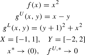
Recall that herein, the test-set from [28] is used, which is in part based on [43–49]; some of the statements are corrected to correspond to the original source and the solution reported in [28]. The examples are defined herein by the host sets \(X,\,Y\), the functions \(f^U,\,g^U,\,\mathbf{g}^L\). Moreover, the analytically obtained optimal solution point(s) \(\mathbf{x}^*\) and infima \(f^{U,*}\) are given; in cases where the minimum is not attained, the notation \(\rightarrow \) is utilized.
-
1.

-
2.

-
3.

-
4.
-
5.

-
6.

-
7.

-
8.

-
9.

-
10.

-
11.

-
12.

-
13.

-
14.

-
15.

-
16.


Appendix B: Relation of assumptions with literature assumptions
1.1 Appendix B.1: Closure versus lower-level Slater point
For convergence of the lower bounding procedure, [28] introduced an assumption which is similar to the one made in [32] for bilevel programs, i.e., that so-called superoptimal (infeasible) points can be excluded by a lower-level point which is a Slater point in the lower level program.
Assumption 4
For (infeasible) points \(\bar{\mathbf{x}} \in X\) that satisfy \(f^U(\bar{\mathbf{x}})< f^{U,*}\) there exists \(\bar{\mathbf{y}}\in Y\), s.t., \(g^U(\bar{\mathbf{x}},\bar{\mathbf{y}})>0\) and \(\mathbf{g}^L(\bar{\mathbf{x}},\bar{\mathbf{y}})<0\).
Assumption 4 directly implies that the infimum of the original problem (GSIP) is equal to the optimal objective value of the relaxation (GSIP-REL). The following (trivial) example shows that Assumption 4 is stronger than requiring the same objective value for the two problems, i.e., Assumption 2 required herein.
Example 1
Consider
The point \(y=0\) is the only lower-level feasible point, thus imposing the constraint \(x \ge 0\). Therefore, the GSIP is feasible for \(x\ge 0\) and thus has the optimal solution point \(x=0\) with an optimal objective value of \(0\). The feasible set is closed. The relaxation (GSIP-REL-SIP) is given by
which also gives \(x \ge 0\) and thus has the same optimal objective value, satisfying Assumption 2. In contrast, there are superoptimal infeasible points \(x<0\) violating the upper level constraint but there is no lower-level Slater point to demonstrate this, thus violating Assumption 4.
1.2 Appendix B.2: GSIP Slater point versus local minimum
Herein, we prove that the assumption on existence of GSIP Slater points in [27, 28] is in essence equivalent with the assumptions made in [18] for SIP and in [39, 40] for pessimistic bilevel programs. Thus, both are stronger than Assumption 3 made herein.
The proofs in [27, 28] require the following assumption:
Assumption 5
There exist GSIP Slater points close to the minimizers \(\mathbf{x}^*\), i.e., for any \(\delta >0\) there exists point \(\mathbf{x}^S\), s.t.
For a GSIP the assumption made in [18, 39, 40] would read:
Assumption 6
There exists an optimal solution \(\mathbf{x}^*\) of the closure of (GSIP) that is not a local minimum of value \(0\) of the function
These assumptions are equivalent, i.e.,
Proposition 1
If (GSIP) is feasible, Assumptions 5 and 6 are equivalent.
Note that feasibility of (GSIP) is equivalent with a nonempty closure of the feasible set.
Proof
First we prove by contraposition that if (SC) holds, so does (AC). Assume that Condition (AC) does not hold, i.e., let \(\mathbf{x}^*\) be an optimal point of the closure of (GSIP) which is a local minimum of value 0 of (AC). Then, there exists a \(\delta >0\), such that for all \(\mathbf x\) with \(||\mathbf{x}-\mathbf{x}^*||<\delta \)
Then, there exists a \(\mathbf{y}\in Y\) with \(\mathbf{g}^L(\mathbf{x}^S,\mathbf{y})\le \mathbf{0}\) and \(g^U(\mathbf{x}^S,\mathbf{y})\ge 0\), contradicting Assumption 3.
Now assume (AC) holds. Then, for every \(\delta >0\), there exists an \(\mathbf{x}^S\) with \(||\mathbf{x}^S-\mathbf{x}^*||<\delta \) such that
That is, for every \(\mathbf{y}\in Y,\,\exists j, g_j^L(\mathbf{x}^S,\mathbf{y})>0\) or \(g^U(\mathbf{x}^S,\mathbf{y})<0\) proving (SC). \(\square \)
Rights and permissions
About this article
Cite this article
Mitsos, A., Tsoukalas, A. Global optimization of generalized semi-infinite programs via restriction of the right hand side. J Glob Optim 61, 1–17 (2015). https://doi.org/10.1007/s10898-014-0146-6
Received:
Accepted:
Published:
Issue Date:
DOI: https://doi.org/10.1007/s10898-014-0146-6