
Abstract
This chapter is intended to enhance the original Overall Equipment Effectiveness (OEE). Calculating plant/equipment OEE can be very helpful for monitoring trends (such as whether a given plant is improving OEE over time) or as a rough measure of where a manufacturng plant lies in the OEE benchmarking spectrum. OEE concept in Total Productive Maintenance (TPM) implementation truly reduces manufacturing complexity into simple, intuitive presentation of information. The proposed approaches establish the functional technique for improvement of the effectiveness of production lines operating and dealing with uncertainty of the six major losses to OEE. The losses associated with production and limits for that losses are the major indexes of the production line performance, because it enables direct evaluation of production line output. The OEE is the process, which is acquired to specify an equivalent weight setting of every single element, even if, each concerning losses are totally different. Hence, the study proposes a weighted approach, to identify dissimilarity in weighting of each OEE element. Theoretical values for the losses improve the measurement of the OEE and Fuzzy analysis can help the decision makers to assess OEE for plant performances. Further, proposed fuzzy methodology can be used to reduce the indecisiveness. Therefore this technique introduces fuzzy theory for OEE computation and will also assist decision makers to evaluate uncertainty and imprecision. The proposed concepts are used to find the OEE for the manufacturing plant, as well as to set the target for the plant and the area to focus for their improvement.
Access provided by Autonomous University of Puebla. Download chapter PDF
Keywords
- Availability
- Decision making
- Fuzzy analysis
- OEE
- Performance rate
- Production losses
- Quality rate
- Signed rating
- TPM effectiveness
- Weighted rating
1 Introduction
In the highly competitive manufacturing environment prevailing at the global level, manufacturing plants of any country or region should be benchmarked and maintained at world-class level. Failing to do that, a plant may be exposed to various difficulties. The results of implementation of Total Productive Maintenance (TPM) program increased plant efficiency and productivity significantly by means of eliminating the major losses [1, 2–4], i.e., the total elimination of all six major losses, including breakdowns, equipment setup and adjustment losses, idling and minor stoppages, reduced speed, defects and rework, spills, process upset conditions, startup and yield losses.
1.1 Major Losses and Performance Evaluation
The Table 1 lists the Six Big Losses, and shows how they relate to the OEE Loss categories. World Class OEE is considered to be 85 % [5] or better. Clearly, there is room for improvement in most manufacturing plants. One of the major goals of TPM implementation and OEE computation is to eliminate or reduce the Six Big Losses—the most common causes of efficiency loss in manufacturing. Worldwide studies indicate that the average OEE rate in manufacturing plants is 60 % [5–7].
1.2 OEE and Its Significance
OEE is a “best practices” way to monitor and improve the manufacturing plants improvement and effectiveness of the manufacturing processes (i.e. machines, manufacturing cells, assembly lines). OEE is simple and practical. It takes the most common and important sources of manufacturing productivity loss, places them into three primary categories and distills them into metrics that provide an excellent gauge for measuring where and how to improve [8].
In general, OEE is calculated as the product of its three contributing factors:
Overall Equipment Effectiveness
where,
- A:
-
Availability of the machine. Availability is proportion of time, a machine is actually available to the scheduled time i.e., it should be available for work.
- P:
-
Performance Rate i.e., P = RE × SR
- Q:
-
Quality rate is percentage of good parts out of total production, sometimes called yield.
- RE:
-
Rate Efficiency is actual average cycle time which is slower than design cycle time because of jams. Output is reduced because of jams.
- SR:
-
Speed Rate is actual cycle time which is slower than design cycle time; machine output is reduced because it is running at a reduced speed.
In other words, OEE can be expressed as follows,
OEE truly reduces complex production problems into simple, intuitive presentation of information. It helps to systematically improve the process with easy-to-obtain measurements.
OEE begins with Planned Production Time and scrutinizes efficiency and productivity losses that occur, with the goal of reducing or eliminating these losses. There are three general categories of loss to consider—Down Time Loss, Speed Loss and Quality Loss.
The proposed approaches give the mathematical approach for computing the Overall Equipment Effectiveness (OEE), i.e. plant effectiveness. OEE is essentially the ratio of Actual Productive Time to Planned Production Time.
The proposed approach assists decision makers to evaluate uncertainty and imprecision. Also to obtain improved OEE measurements as well as producing better production improvement plans and lean manufacturing implementation strategy. In general OEE (F) can be expressed as “n” number of factors namely f1, f2… fn.
In the above mentioned case, n = 3 where f1 = Availability (A), f2 = Performance (P), and f3 = Quality (Q).
OEE measurement is an effective way of analyzing the efficiency of a single machine or an integrated manufacturing system. OEE incorporates availability performance rate and quality rate and gives results. In other words, OEE addresses all losses caused by the equipment, not being available when needed due to breakdowns or set-up and adjustment losses, not running at the optimum rate due to reduced speed or idling and minor stoppage Losses and not producing first quality output due to defects and rework or start-up losses. A key objective of TPM is cost efficiency; maximizing Overall Equipment Effectiveness through the elimination or minimization of all these six losses by means of lucid approach.
The OEE is not that which gives one magic number; it gives three numbers other than OEE, which are all useful individually as the situation changes from day to day. In addition, it helps to visualize performance in simple terms—a very practical simplification. The OEE is probably the most important tool in continuous improvement program in manufacturing industry. Through the OEE analysis the operators can observe, where they lose most of the production (The six Major Losses as mentioned in above).
Significant improvement can be evident within a short period by means of eliminating the six major losses with result of enhanced maintenance activities and equipment management.
Increasingly, companies working in process manufacturing environments are discovering a surprisingly effective framework from which to tackle the continuous improvement challenge: the “Six Big Losses” approach. Developed in the 1970s by the Japan Institute of Plant Maintenance (JIPM), the Six Big Losses framework enables manufacturers to examine their efficiency problem with an unprecedented level of granularity According to JIPM, the OEE is based on three main aspects; each element concerns with different losses as shown in the Table 1.
2 OEE: Weighted Approach
2.1 OEE and its Computation Method
As described in World Class OEE, the OEE calculation is based on the three OEE Factors, Availability, Performance, and Quality. Here’s how each of these factors is calculated [1, 5].
2.1.1 Availability
Availability takes into account Down Time Loss, and is calculated as:
Availability = Operating Time/Planned Production Time
2.1.2 Performance
Performance takes into account Speed Loss, and is calculated as:
Performance = Ideal Cycle Time/(Operating Time/Total Pieces)
Ideal Cycle Time is the minimum cycle time that your process can be expected to achieve in optimal circumstances. It is sometimes called Design Cycle Time, Theoretical Cycle Time or Nameplate Capacity. Since Run Rate is the reciprocal of Cycle Time, Performance can also be calculated as:
Performance = (Total Pieces/Operating Time)/Ideal Run Rate
Performance is capped at 100 %, to ensure that if an error is made in specifying the Ideal Cycle Time or Ideal Run Rate the effect on OEE will be limited.
2.1.3 Quality
Quality takes into account Quality Loss, and is calculated as:
Quality = Good Pieces/Total Pieces
2.1.4 OEE
OEE takes into account all three OEE Factors, and is calculated as:
OEE = Availability × Performance × Quality
2.2 Need of OEE: Weighted and Fuzzy Approaches
Formerly, lots of research has been done to customize and fine tune the OEE computation Formula, i.e. OEE = A × P × Q (specific to their plants/task). But there was no research was done based on the fixation of contributing factors and its effect on the OEE. So there was a chasm for real time values and targets fixed, that can be narrow down by appropriate method, for that this ideology will help the manufacturing industries to work on.
2.3 Weighted Rating for A, P and Q
In proposed system, OEE is considered as a signed graph, where each factors BD, SA, MI, RS, RL and SL are assigned with weight ratings based on the loss percentage. Signed weight [9, 10] (++, +−, −+, −−) is attached to each factors of the graph based on the combination of above contributing factors for A, P, Q and OEE. Depending upon the BD, SA, MI, RS, RL and SL ratings A, P and Q are calculated. Similarly based on A, P and Q ratings OEE is estimated.
2.4 Existing Weighted Rating for A, P and Q
In a weighted graph, A1, A2, A3 and A4 are considered as the loss ratings, where A1 < A2 < A3 < A4. (i.e., A1 is the lowest loss level rating and A4 is the highest loss level rating) [10–13].The ratings for the basic six parameters differ from one another based on user. In the subsequent ranking scheme, more weight-age is given for BD i.e., up to 10 % loss, where as other parameters have less weight-age of 2–3 %, [14] (Following set of data for model case plant limits values in %).
1. BD—Breakdown a. A1 = 0 to ≤ 1 b. A2 = > 1 to ≤ 5 c. A3 = > 5 to ≤ 10 d. A4 = > 10 | 2. SA—Setup adjustment a. A1 = 0 to ≤ 0.5 b. A2 = > 0.5 to ≤ 1 c. A3 = > 1 to ≤ 2 d. A4 = > 2 |
3. MI—Minor/Idling stoppages a. A1 = 0 to ≤ 1 b. A2 = > 1 to ≤ 2 c. A3 = > 2 to ≤ 3 d. A4 = > 3 | 4. RS—Reduced speed a. A1 = 0 to ≤ 1 b. A2 = > 1 to ≤ 2 c. A3 = > 2 to ≤ 3 d. A4 = > 3 |
5. RL—Reject / Rework losses a. A1 = 0 to ≤ 0.5 b. A2 = > 0.5 to ≤ 1 c. A3 = > 1 to ≤ 2 d. A4 = > 2 | 6. SL—Start-up losses a. A1 = 0 to ≤ 0.5 b. A2 = > 0.5 to ≤ 1 c. A3 = > 1 to ≤ 2 d. A4 = > 2 |
3 Program Dependence Graph
A Program Dependence Graph (PDG) is a suitable internal program representation for monolithic programs for the purpose of carrying out certain engineering operations such as scheming and computation of program metrics [13, 15] (Figs. 1, 2).

PDG block diagram for OEE

Flow chart for current OEE
-
(a)
In the following flow diagram, stage 1 calculation of availability with the inputs BD and SA with constrain limit shown in Fig. 3.
Fig. 3 
Flow chart for availability calculation
-
(b)
In stage 2, calculation of performance with the inputs of MI and RS with constrain limit shown in the Fig. 4.
Fig. 4 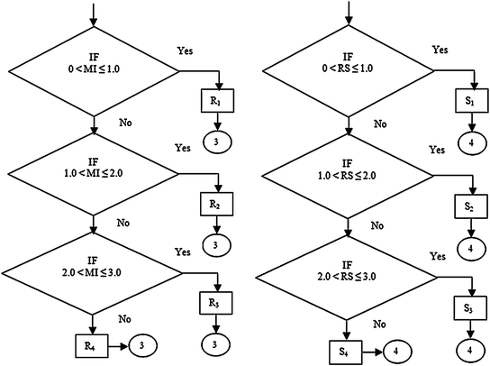
Flow chart for performance calculation
-
(c)
In stage 3, calculation of quality with the inputs of RL and SL with constrain limit as in Fig. 5.
Fig. 5 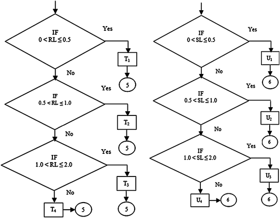
Flow chart for quality calculation
-
(d)
Determination of OEE assigned as below OEE = Pi x Qi x Ri x Si x Ti x Ui.
-
Stage 1: Calculation of Availability
-
Stage 2: Calculation of Performance
-
Stage 3: Calculation of Quality
-


4 Signed Approach for OEE
Signed weight [10] with following constrained users fixed methodology ++, +−, −+, −− are fixed for best, better, good, worst ratings for A, P, Q and OEE is based on the combination of above contributing factors of A, P, Q and OEE. The BD, SA, MI, RS, RL and SL are assigned with signed ratings to allocate A, P and Q values. Similarly based on A, P and Q signed ratings OEE values are predicted [14] (Tables 2, 3, 4).
5 Fuzzyfication Algorithm for Current OEE
5.1 Programming Algorithm
For various A, P and Q values [1, 100], OEE computed and classified using following algorithm.
-
Step 1: Start the process
-
Step 2: Fix A = 0
-
Step 3: Fix P = 0
-
Step 4: Fix Q = 0
-
Step 5: Calculate OEE = A × P × Q
-
Step 6: Pre-processing
-
Step 7: Rotate Step 5 to Step 6 until Q ≤ 100 with the step value of Q
-
Step 8: Rotate Step 4 to Step 7 until P ≤ 100 with the step value of P
-
Step 9: Rotate Step 3 to Step 8 until A ≤ 100 with the step value of A
-
Step 10: Stop the process
Note: In Pre–processing the constrains for A, P and Q are being fixed with plant required strategies. As stated in Sect. 2. The step values with respect to necessitate.
5.2 Approximation Analysis for Current OEE
From the fuzzy analysis for the OEE in % using the formula [OEE = A × P × Q], even though the A, P, Q values are below the targeted values Still OEE values or above the 85 %, the world class OEE value as target value. From the reading it’s giving basic guidelines for setting the minimum criteria for A, P and Q values. The guiding principles are as follows;
5.2.1 Individual Constraint for Variables
5.2.2 Combine Constraint for Variables
So the target setting for a particular industry may use this as basic guidelines and set A, P and Q values based on their current performance results with benchmarked OEE.
For various A, P and Q values [1, 100], OEE computed and classified using following algorithm.
In a weighted graph, A1, A2, A3 and A4 are considered as the loss ratings, where A1 < A2 < A3 < A4. (i.e., A1 is the lowest loss level rating)
5.3 Boundaries for A, P and Q
For setting maximum (extreme) level values for A, P and Q for current bench mark OEE target is as follows.
5.3.1 Extreme Level
In this case one of the factors as minimum at benchmark setup and other two at maximum (100 %).
5.3.2 Average Level
In the average order case with equal rating at 95 % can be articulated.
6 Real Time Application
OEE data collection, analysis and reporting provide the principal basis for improving equipment effectiveness by eliminating the major equipment-related losses. The weighted approach for OEE calculation is presented and the analytical hierarchy process has been applied for setting the weight of all the factors namely BD, SA, MI, RS, RL and SL. The prospective of the proposed method can be applied for new as well as existing manufacturing plants. OEE data very quickly leads to root-cause identification and elimination of losses for plant performance improvement. Overall Equipment Effectiveness continues to gain acceptance as an effective method to measure production floor performance.
Capturing reliable production floor information is critical for producing reliable OEE focused progress of the plant or equipment. It will be optimal tool for plants implementing TPM. This weighted approach and OEE results will be benchmarking tool to gauge manufacturing system, especially maintenance management system. OEE helps manufacturer to improve productivity and get better visibility of the operations and also allow management to take sound decisions.
7 Conclusion and Future Work
The proposed methodology through algorithmic approach to get computational work, the values of OEE categorized through fuzzy logic method on A, P and Q to get optimization.
No manual data collection or manual compilation for OEE calculations is the first step in improving both the accuracy of OEE reports as well as reducing the cost to produce the reports through neural network.
The utility of artificial neural network models lies in fact that, they can be used to infer for future purposes.
Abbreviations
- A:
-
Availability
- BD:
-
Break-Down
- JIPM:
-
Japan Institute of Plant Maintenance
- MI:
-
Minor/Idling stoppages
- OEE:
-
Overall Equipment Effectiveness
- P:
-
Performance rate
- PE:
-
Plant Effectiveness
- Q:
-
Quality rate
- RL:
-
Reject/rework Losses
- RS:
-
Reduced Speed
- SA:
-
Setup Adjustment
- SL:
-
Start-up Losses
- TPM:
-
Total Productive Maintenance
References
Nakajima S (1988) Introduction to TPM. Productivity Press, Cambridge
Venkatesh J (2005) An introduction to total productive maintenance (TPM), The plant maintenance resource center, pp 2–3, 15–27
Wireman T (1990) World class maintenance management. Industrial Press, New York
Yamashina H (1995) Japanese manufacturing strategy and the role of total productive maintenance. J Qual Maint Eng 1(1):27–38
Lungberg O (1998) Mearsument of overall equipment effectiveness as a basic for TPM activities. Int J oper Prod Manag 18(5):495–507
Lesshammar M (1999) Evaluation and improvement of manufacturing performance measurement systems—the role of OEE. Int J Oper Prod Manag 19(1):55–78
Dal B, Tugwell P, Greatbanks R (2000) Overall equipment effectiveness as a measure of operational improvement. Int J Oper Prod Manag 20(12):1488–1520
Yu B, Singh MP (2002) An evidential model for distributed reputation management, AAMAS’02, Bologna, Italy, 15–19 July 2002
Thiagarajan K, Raghunathan A, Natarajan P, Poonkuzhali G, Ranjan P (2009) Weighted graph approach for trust reputation management. World Acad Sci Eng Technol 32:830–836
Yu B, Singh MP (2000) Trust and reputation management in a small- world network. In: proceedings of the 4th international conference on multiagent systems, pp 449–450
Yu B, Singh MP (2000) A social mechanism of reputation management in electronic communities. In: proceedings of the 4th international workshop on cooperative information agents
Harary F (1969) Graph theory. Addision-Wesley, Reading
Maran M, Manikandan G, Thiagarajan K (2012) Overall Equipment effectiveness measurement by weighted approach method. In: Lecture notes in engineering and computer science: proceedings of the international multi conference of engineers and computer scientists 2012, IMECS 2012, 14–16 March, Hong Kong, pp 1280–1285
Srinivasan SP, Malliga P, Thiagarajan K (2008) An Algorithmic graphical approach for ground level logistics management of Jatropha seed distribution. Ultra Sci Phys Sci 20(3):605-612
Acknowledgments
The authors would like to thank Dr. Ponnammal Natarajan, Former Director of Research, Anna University, Chennai, India. Currently Advisor (Research and Development), Rajalakshmi Engineering College, for her intuitive ideas and fruitful discussions with respect to the paper’s contribution and the Management of Velammal College of Engineering and Technology, Madurai and Dr. R. Vivekaanandhan, Assistant Professor, Department of English, Velammal College of Engineering and Technology, Madurai, for his constant encourage and support to complete the task.
Author information
Authors and Affiliations
Corresponding author
Editor information
Editors and Affiliations
Rights and permissions
Copyright information
© 2013 Springer Science+Business Media Dordrecht
About this chapter
Cite this chapter
Maran, M., Manikandan, G., Thiagarajan, K. (2013). Overall Equipment Effectiveness Measurement: Weighted Approach Method and Fuzzy Expert System. In: Yang, GC., Ao, SI., Huang, X., Castillo, O. (eds) IAENG Transactions on Engineering Technologies. Lecture Notes in Electrical Engineering, vol 186. Springer, Dordrecht. https://doi.org/10.1007/978-94-007-5651-9_17
Download citation
DOI: https://doi.org/10.1007/978-94-007-5651-9_17
Published:
Publisher Name: Springer, Dordrecht
Print ISBN: 978-94-007-5623-6
Online ISBN: 978-94-007-5651-9
eBook Packages: EngineeringEngineering (R0)